Coordinated Followup Could Have Enabled the Discovery of the GW190425 Kilonova

Abstract

The discovery of a kilonova associated with the GW170817 binary neutron star merger had far-reaching implications for our understanding of several open questions in physics and astrophysics. Unfortunately, since then, only one robust binary neutron star merger was detected through gravitational waves, GW190425, and no electromagnetic counterpart was identified for it. We analyze all reported electromagnetic followup observations of GW190425 and find that while the gravitational-wave localization uncertainty was large, most of the 90% probability region could have been covered within hours had the search been coordinated. Instead, more than 5 days after the merger, the uncoordinated search covered only 50% of the probability, with some areas observed over 100 times, and some never observed. We further show that, according to some models, it would have been possible to detect the GW190425 kilonova, despite the larger distance and higher component masses compared to GW170817. These results emphasize the importance of coordinating followup of gravitational-wave events, not only to avoid missing future kilonovae, but also to discover them early. Such coordination, which is especially important given the rarity of these events, can be achieved with the Treasure Map, a tool developed specifically for this purpose.

1 Introduction

Binary neutron star (BNS) mergers were predicted to produce both gravitational waves (GWs; Clark & Eardley, 1977) and electromagnetic (EM) radiation. The latter was theorized to be emitted in the form of two types of transients: a short gamma-ray burst (GRB; Eichler et al., 1989), and longer-duration emission from the radioactive decay of heavy elements synthesized via the $r$-process in the ejecta (Li & Paczyński, 1998). This transient has been nicknamed “macronova” (Kulkarni, 2005) or “kilonova” (Metzger et al., 2010).

All three predictions were confirmed with the first discovery of a GW signal from a BNS merger, GW170817, detected and localized by the Advanced Large Interferometer Gravitational-wave Observatory (LIGO; LIGO Scientific Collaboration et al., 2015), and the Advanced Virgo detector (Acernese et al., 2014), during their second observation run (O2), on August 17, 2017 (Abbott et al., 2017a). The GW source was localized to a region of $\sim 30\ deg^{2}$ at a distance of $\sim 40\ Mpc$ and had a total binary mass of $2.74^{+0.04}_{-0.01}\ M_{\odot}$ (Abbott et al., 2017a). A short GRB, GRB170817A, consistent with the GW localization, was detected $\sim$2 seconds after the GW-determined merger time (Abbott et al., 2017b) by the Fermi Gamma-ray Burst Monitor (Fermi-GBM; Meegan et al., 2009), and the International Gamma-Ray Astrophysics Laboratory (INTEGRAL; Winkler et al., 2003). An optical transient, AT 2017gfo, also consistent with the GW localization, was detected 11 hours later (Coulter et al., 2017a). Both EM transients were later confirmed to be physically associated with the BNS merger (Abbott et al., 2017).

Specifically, AT 2017gfo was consistent with kilonova predictions whereby at the coalescence of a BNS system, $10^{-4}-10^{-2}M_{\odot}$ of neutron-rich material are ejected at velocities of $0.1-0.3c$ in the equatorial plane due to tidal effects (e.g. Rosswog et al., 1999; Hotokezaka et al., 2013). Additional mass was predicted to be ejected in the polar direction from the contact region at the time of the merger (e.g. Bauswein et al., 2013; Hotokezaka et al., 2013). Lanthanides formed in low electron-fraction material, such as the equatorial tidal ejecta, have a high opacity (Kasen et al., 2013; Tanaka & Hotokezaka, 2013), making the light curve redder, fainter, and longer lived compared to low lanthanide ejecta (Barnes & Kasen, 2013; Grossman et al., 2014), such as that from to polar regions. The result, seen in AT 2017gfo, is a kilonova of at least two components: one blue and short-lived from the lanthanide-poor ejecta, and one red and longer-lived from the lanthanide-rich ejecta. For a review of this event, see for e.g. Nakar (2020) and Margutti & Chornock (2021).

GW170817 and its EM counterparts confirmed that BNS mergers are sites of $r$-process nucleosynthesis (e.g. Kasen et al., 2017), and confirmed the connection between short GRBs and BNS mergers. This event also demonstrated a novel method to constrain the Hubble constant (Abbott et al., 2017). However, many open questions regarding the properties of the kilonova emission remain, such as whether the source of the early blue emission is indeed a distinct lanthanide-poor ejecta component (other physical mechanisms were proposed, e.g. Kasliwal et al., 2017; Piro & Kollmeier, 2018; Waxman et al., 2018). More BNS detections and multi-wavelength observations of their EM counterparts, especially during the first few hours (e.g. Arcavi, 2018) are needed to answer these questions.

The second (and so far, last) robust GW detection of a BNS merger occurred at the start of the third GW-detector observing run (O3). GW190425 was discovered on April 25, 2019, at 08:18:05 UTC, at a distance of $159^{+69}_{-72}\ Mpc$ and with a total binary mass of $3.4^{+0.3}_{-0.1}\ M_{\odot}$ (Abbott et al., 2020). The event was detected only by a single LIGO detector, making its localization poorly constrained, with a $10183\ deg^{2}$ 90% uncertainty region initially (Ligo Scientific Collaboration & VIRGO Collaboration, 2019a). This region shrank about one day later to $7461\ deg^{2}$ (Ligo Scientific Collaboration & VIRGO Collaboration, 2019b), but grew back to $9881\ deg^{2}$ in the final localization published in the second GW Transient Catalog (GWTC-2; Abbott et al., 2021). The localization parameters are summarized in Table 1, and the localization maps are shown in Figure 1.

No coincident GRB was detected by the Fermi Large Area Telescope (Fermi-LAT; Atwood et al., 2009; Axelsson et al., 2019), the Swift Burst Alert Telescope (Swift/BAT; Gehrels et al., 2004; Sakamoto et al., 2019) nor by the Fermi-GBM (Fletcher et al., 2019). The INTErnational Gamma-Ray Astrophysics Laboratory (INTEGRAL; Winkler et al., 2003) reported a detection of a low significance signal, associated with a BNS merger (Pozanenko et al., 2020), but with no localization information to robustly tie it to GW190425 (Savchenko et al., 2019).

Table 1: GW190425 localization areas and distances.

Epoch	Date	90% Area	50% Area	Distance
	[UTC]	[$deg^{2}$]	[$deg^{2}$]	[Mpc]
Initial	2019-04-25	10183	2806	$154\pm 45$
Alert	08:19:27
Update	2019-04-26	7461	1378	$156\pm 41$
Alert	10:48:17
GWTC-2	2020-07-27	9881	2400	$157\pm 43$
	16:41:49

Note. — “90% (50%) Area” refers to the sky area that contains 90% (50%) of the probability for the location of the source.

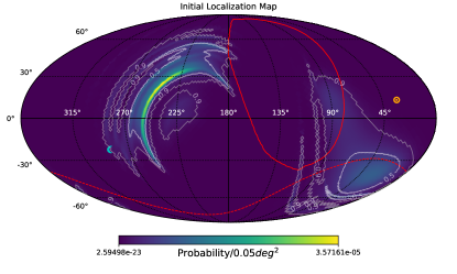
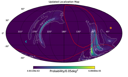
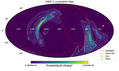
Figure 1: GW190425 localizations released in the initial (top) and update (middle) alerts, and in the final GWTC-2 publication (bottom; Abbott et al., 2021). White and grey contours denote the regions containing 50% and 90% of the probability of the source location, respectively. The Swift/Bat and Fermi-LAT footprints at the time of the merger are presented in red solid and dashed lines, covering areas of $4596\ deg^{2}$ and $8602\ deg^{2}$, respectively. The position of the Sun and Moon at the time of the merger are denoted in their respective symbols.

An extensive EM followup effort to find the kilonova associated with GW190425 began shortly after the initial alert. However, no significant kilonova candidate was identified. This was attributed to the larger distance, higher component masses, more equal mass ratio, and to the larger localization compared to GW170817 (e.g. Hosseinzadeh et al., 2019a; Lundquist et al., 2019; Abbott et al., 2020; Foley et al., 2020; Gompertz et al., 2020; Kyutoku et al., 2020; Sagués Carracedo et al., 2021; Camilletti et al., 2022; Dudi et al., 2022; Radice et al., 2024). However, here we show that, according to some models, the emission from the GW190425 kilonova could have been detected by existing facilities, and that most of the localization could have been covered within hours, had the EM followup effort been coordinated.

Coordinating EM followup of GW events is challenging. Reports of observations and possible kilonova candidates during O2 and O3 were primarily communicated through GRB Coordinates Network (GCN; now the General Coordinates Network) circulars. GCN circulars were designed to be human readable, with no unified text format. As such they are not ideal when reporting lists of coordinates, bands, and sensitivities observed. The non machine-readable format makes it very difficult to parse, store and interpret such information in real time.

One tool designed to address the challenge of coordinating EM followup of GW events is the Treasure Map (Wyatt et al., 2020). Treasure Map is a web application that collects, stores and distributes followup reports through a machine-friendly Application Programming Interface (API). The API allows observers to report their planned and executed observations and to retrieve those of other facilities in order to inform their own counterpart search plan in real time. In addition, an interactive visualization allows observers to see their observations and those of other facilities on a map, together with GW localization in an intuitive way. All of the reports are also available to download at a later date for analyzing followup efforts and non-detection statistics. Unfortunately, the Treasure Map did not exist during GW190425, leading to very inefficient followup, as we will show here. Our goal is to encourage the community to use tools such as the Treasure Map during the next BNS merger, in order to increase the chances of finding the EM counterpart, and to do so as quickly as possible. We do so by demonstrating the impact of uncoordinated observations on missing the counterpart to GW190425.

In this work, we analyze all reported infrared, optical and ultraviolet followup efforts of GW190425. In Section 2 we describe our data sources and collection process; in Section 3, we analyze the sky coverage and depth achieved in the context of the expected kilonova emission from this event; and, finally, in Section 4, we discuss our conclusions.

2 Data

In order to analyze the efficiency of the search for the GW190425 EM counterpart we collected pointing and photometric data of infrared, optical and ultraviolet observations obtained as followup of GW190425 up to 2019 April 30, 23:57:21 UTC, which were reported in one of the following sources (removing duplicate reports of the same observations): The Treasure Map (1419 observations reported retroactively), 122 GCN circulars (1339 observations), the MASTER global robotic net (MASTER-Net; Lipunov et al., 2010) website (4491 observations), the Coulter et al. (2024) report on the One-meter Two-hemispheres (1M2H) followup (345 observations), and the Smartt et al. (2024) report of the Panoramic Survey Telescope and Rapid Response System (PAN-STARRS) and the Asteroid Terrestrial-impact Last Alert System (ATLAS) followup (6631 observations). In total, 14255 unique observations were collected, including time stamps, limiting magnitudes, and bands used. Instrument footprints and fields of view (FOVs) were taken from the Treasure Map when available, from GCN reports when provided there, and from instrument-specific websites and publications otherwise (all references are provided in Table 2). Some galaxy-targeted searches provided target galaxy names rather than exact coordinates pointed to. In such cases, we obtained the galaxy coordinates from the Galaxy List for the Advanced Detector Era (GLADE) catalog (Dálya et al., 2018) or the SIMBAD Astronomical Database (Wenger et al., 2000) and assumed the target galaxies were positioned at the center of the observed footprint. A summary of the observations and instruments used in this analysis is presented in Table 2, and the full list of all pointings gathered is presented in Table 3.

Table 2: GW190425 EM followup observations reported in circulars, the Treasure Map, by MASTER-Net on their website, and in Coulter et al. (2024) and Smartt et al. (2024), out to 5.65 days after merger.

Group/Facility/Instrument	No. of	Bands	Field of View	Median $5\sigma$ Depth	Pointings Reference
	Pointings		[$deg^{2}$]	[AB Mag]
Pan-STARRSa	6209	w,i,z	7.07	21.58	1
MASTER-Netb	4491	Clear	8.00	19.10	2
ZTFc	596	g,r,i	46.73	21.05	3
ATLASd	422	o,c	28.89	19.26	1
Swift/UVOTe	392	u	8.0e-02	19.40	3
GOTOf	303	V,g	18.85	19.85	3
J-GEM/Subarug	154	r	2.0e-03	24.00	4
1M2H/Swopeh	151	B,V,u,g,r,i	0.25	21.55	5
COATLIi	128	w	3.3e-02	n/a	6
KMTNet 1.6mj	120	R	4.00	n/a	7
KAITk	101	Clear	1.2e-02	19.00	8
Harold Johnson Telescope/RATIRl	99	J,H,Y,Z,g,r,i	8.1e-03	20.74	9, 10
GROWTH/LOTm	93	R,g,r,i	3.6e-02	19.79	11, 12, 13
1M2H/Nickeln	93	r,i	1.1e-02	20.24	5
MMTO/MMTCamo	81	g,i	2.0e-03	21.48	3, 14
GWAC-F60Ap	80	Clear	9.0e-02	18.97	15
CNEOSTq	75	R	9.00	19.86	16
BOOTES-5r	63	Clear	2.78	20.50	17
SAGUARO/CSS 1.5ms	61	Clear	5.00	21.30	3
LCO 1mt	58	g,r,i	0.20	21.30	18, 19, 20, 21
1M2H/Thacheru	53	g,r,z	0.12	19.55	5
GRANDMA/LesMakes T60v	52	Clear	17.64	19.20	22
GRANDMA/AZT$-$8w	52	B,R	0.25	19.00	22
GRANDMA/Abastumani T70x	40	R	0.25	16.29	22
Xinglong 60/90cmy	35	Clear	2.25	18.00	23
McDonald Observatory 2.1m/CQUEANz	30	i	6.1e-03	20.44	24
1M2H/ANDICAM-CCDaa	27	I	1.1e-02	20.70	5
GROWTH/Kitt Peak 2.1m/KPEDab	25	I,g,r	7.0e-03	20.40	25, 26, 27
YAHPTac	23	R	3.4e-02	18.18	28
1M2H/ANDICAM-IRad	21	J,H,K	1.5e-03	13.45	5
Liverpool Telescope/IO:Oae	19	g,r,i,z	2.8e-02	22.24	29, 30
LOAO 1maf	13	R	0.22	19.23	31
GROWTH-Indiaag	10	g,r,i	0.49	18.41	32, 33
Konkoly 0.8mah	10	g,r	9.0e-02	20.40	34
IRSF 1.4m/SIRIUSai	7	J,H,K	1.6e-02	15.31	35, 36
TAROT TREaj	7	R	17.64	17.23	37
Konkoly 0.6/0.9mak	5	Clear	1.36	21.50	34
Lijiang 2.4mal	5	g,r	2.56	19.04	38
GRANDMA/CAHA 2.2mam	5	U,B,V,R,I	4.5e-02	22.30	39
DECaman	4	g,r,i,z	3.35	23.85	40
MPG/GRONDao	3	r,i,z	8.1e-03	20.00	41
NOT/ALFOSCaq	3	g,r,i	1.1e-02	20.39	42
OSN 1.5mar	2	R	6.8e-02	21.30	43, 44
ANU/SkyMapperas	2	i	5.62	20.00	45
GTC/OSIRISat	1	r	1.8e-02	22.80	44
VISTA/VIRCAMau	1	K	2.14	19.55	46

Note. — Some sources did not provide their observation depths. These are marked with “n/a” in the depth column.

Table 3: List of the observations used in this work.

Facility/Instrument	MJD	R.A. [deg]	Dec. [deg]	Band	$5\sigma$ Limiting Mag.	Source
ZTF	58598.3460	180.0000	62.1500	r	20.46	Treasure Map
ZTF	58598.3465	-168.6100	54.9500	r	20.95	Treasure Map
ZTF	58598.3470	-165.0502	47.7500	r	21.05	Treasure Map
ZTF	58598.3474	-167.7500	40.5500	r	20.80	Treasure Map

Note. — This table is published in its entirety in the machine readable format. A portion is shown here for guidance regarding its form and content.

3 Analysis and Results

In order to measure the efficiency of the search for the GW190425 EM counterpart, we first analyze the observability of the GW localization region at the time of the merger (Section 3.1), followed by the amount of the GW localization that was covered as a function of time, in terms of the total probability, area, and galaxy luminosity (Sections 3.2 and 3.3). We then examine the reported non-detection limiting magnitudes and compare them to light curves of the GW170817 kilonova and of kilonova models tuned to the parameters of GW190425 (Section 3.4).

GW localizations are provided as Hierarchical Equal Area isoLatitude Pixelation (HEALPix; Górski et al., 2005) maps. These maps divide the sky into pixels of equal area and assign a probability value for the location of the GW source to each pixel. Each pixel is also assigned a distance to the source (assuming it is at that position) and a distance error estimate. The number of pixels $N_{pixels}$ in the map is $12\cdot(nside)^{2}$ with $nside=2^{n}$ for some integer $n\geq 0$. The localization maps provided for GW190425 have a resolution of $nside=256$, or $N_{pixels}=786432$. This translates into pixels with an area of $0.052\ deg^{2}$ each. We perform all of our analysis using the maps in this resolution, as they were provided, except for the observability analysis (Section 3.1), for which we downsample the maps to $nside=32$ (i.e. $N_{pixels}=12288$ and a pixel area of $3.36\ deg^{2}$) for computational ease.

3.1 Observability

We define that a region on the sky is “visible” at a point in time from a certain location on Earth when the Sun is a least $12^{\circ}$ below the horizon, the Moon separation is at least $20^{\circ}$ (the moon illumination was 66% at the time of the GW190425 merger) and the airmass is less than 2.5. According to this definition, of the $9881\ deg^{2}$ ($2400\ deg^{2}$) of the 90% (50%) final localization, $8182\ deg^{2}$ ($2182\ deg^{2}$), or roughly 83% (90%), were visible during the 24 hours following the merger from the combined locations of all ground-based observatories listed in Table 2.

Next, we define the “accessibility” of each area of the sky to each instrument as the amount of time per day that area is visible to that instrument, $t_{visible}$, weighted by the instrument FOV (to take into account that larger FOV instruments can cover more area simultaneously) and divided by the pixel area of the map ($3.36\ deg^{2}$ in this case):

$$t_{accessibility}=t_{visible}\left(\frac{FOV}{3.36deg^{2}}\right)$$ (1)

We define an inaccessible area as one with total accessibility (i.e. summed over all ground-based instruments considered here) $t_{accessibility}<5\ min$ (corresponding to a typical single exposure time). Using this definition, 6284 $deg^{2}$ of the sky were inaccessible due to sun and moon constraints, of which 2098 $deg^{2}$ were in the GWTC-2 90% localization region. The rest of the localization region, encompassing 75% of the probability, was visible with a median total accessibility time of 41.5 hours. The total accessibility of the 90% localization region during the first day since merger is presented in Figures 2 and 3, and in Table 4.

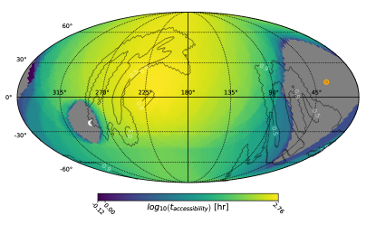
Figure 2: Accessible hours during the first day after the merger summed over all ground-based observatories listed in Table 2. An accessible hour is one that is over an airmass of 2.5 and not sun or moon-constrained, normalized to the FOV of each instrument (see text for details). Grey regions indicate inaccessible areas $(t_{accessibility}<5\ min)$. Black contours are of the GWTC-2 localization. The sun and moon locations in the figure at the time of the merger.

Table 4: GW190425 accessible localization areas and probabilities, and median accessibility.

Epoch	90% Area	Accessible	Accessible	Median
		90% Area	Probability	Accessibility
	[$deg^{2}$]	[$deg^{2}$]		[Hr]
Initial	10183	8216	72%	80.0
Update	7461	5833	76%	32.0
GWTC-2	9881	7783	75%	41.5

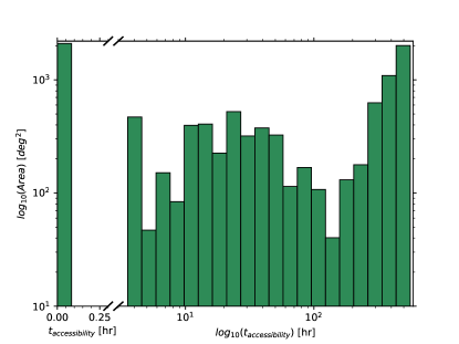
Figure 3: Accessible hours of the GWTC-2 90% localization during the first day after merger. Out of the 90% localization area, 2098 $deg^{2}$ were inaccessible ($t_{accessibility}<5\ min$, leftmost bin), leaving 75% of the probability accessible, with a median total accessibility of 41.5 hours.

3.2 Area and Probability Coverage

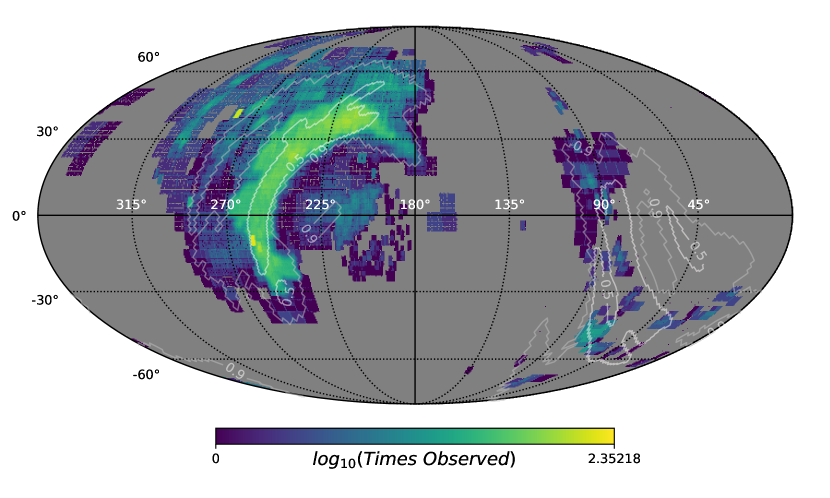
Figure 4: Total number of infrared, optical and ultraviolet followup observations up to 5.65 days post merger for GW190425. Grey areas are where no observations were reported. Lines mark the 50% and 90% probability regions of the final GWTC-2 localization. While some parts of the localization were observed over 100 times, some were not observed at all, even though they were accessible (Figure 2).

We count the sky area and the probability observed up to 5.65 days after the time of the merger, both with and without overlap between observations, in order to measure how much of the localization was covered and how much of it was observed multiple times. Measuring total area and probability on a HEALPix map requires counting the pixels that overlap with an observed footprint. Due to the resolution of the map, the minimal area that can be counted per footprint is $0.052\ deg^{2}$. However, there are footprints with a smaller FOV (as seen in Table 2). Here we use the healpy python package, which includes two methods for counting (“querying”) pixels inside an observed footprint. The “inclusive” method counts every pixel that overlaps with the footprint, while the “exclusive” method only counts pixels that have their center fall inside the footprint. An illustration of these two methods is presented in Figure 8 in Appendix A. We choose the exclusive method for our analysis, as it is a more conservative accounting of the actual area and probability covered, while the inclusive method over counts pixels, causing an overestimation of the area and probability covered.

Figure 4 shows the total coverage of all reported followup observations up to 5.65 days post-merger outlined in Section 2. Some regions, in the northern part of the localization, were observed more than 100 times while most of the accessible southern part of the localization was not observed at all.

The GW localization was updated 26 hours after the initial localization was released. At the time of the update, earlier footprints had their probability coverage changed. We take that into account by retroactively recounting the probability covered by all of the observations using the updated localization from the time it was released. The area covered does not depend on the localization map and thus, no recounting of the area covered is needed at the time of the update. The sum of area and probability covered is performed in two different ways, first without regard to whether observations overlap or not, and second with overlapping regions counted only once. We compare the probability covered to the 100% probability of the entire sky and the area covered to the initial and updated 90% probability areas.

The probability and area covered as a function of time are shown in Figure 5. Within 5.65 days following the merger, 11486 $deg^{2}$ were covered (once or more). This is more than the area of the GWTC-2 90% probability region, but not all of the area covered is in that region (Fig. 4). In fact, at 5.65 days post-merger, only 54% of the probability (of the GWTC-2 localization) was covered, while enough observations were made to cover over 120000 $deg^{2}$ by that time. The 90% probability region could have theoretically been covered within three hours from merger.

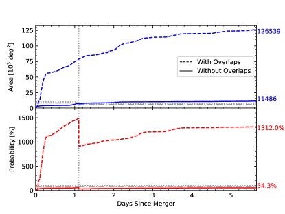
Figure 5: Cumulative area (top) and probability (bottom) observed during the 5.65 days following the GW190425 merger. Colored dashed lines are for all observations (including overlapping ones) while solid lines are for unique positions on the sky (without overlap). Horizontal grey dotted lines denote the total area inside the 90% localization region and 100% probability reported at the time, for the top and bottom plots, respectively, while the grey dash-dotted lines are for the accessible area and probability (see Section 3.1). The vertical grey dotted line denotes the time of the updated localization.

3.3 Galaxy Luminosity Coverage

We define the galaxy luminosity coverage as the fraction of $B$-band luminosity of galaxies observed out of the total $B$-band luminosity of all galaxies with $L>L_{B}^{*}$ in the 90% localization volume within 3$\sigma$ of the mean localization distance. Here, $L_{B}^{*}$ is the $B$-band luminosity corresponding to $L^{*}$, the charactesitic luminosity of the Schechter Function (Schechter, 1976). We adopt a corresponding absolute magnitude in the $B$ band of $M_{B}^{*}=-20.7$, following Arcavi et al. (2017a). The GLADE catalog is less complete to galaxies fainter than $L^{*}$ at large distances (see Dálya et al., 2018, for more details).

We count only galaxies that have a $B$-band apparent magnitude and a distance estimate in Version 2.3 of the GLADE catalog. There are a total of 47664 (34302) such galaxies in the catalog inside the initial (updated) 90% localization.

We count galaxies that are inside observed footprints and the localization volume, once with recounting galaxies and once without. Figure 6 shows the galaxy luminosity coverage as a function of time. After 5.65 days from the merger, only 52% of the $B$-band luminosity in galaxies inside the updated localization region was observed, while 11.88 times the localization luminosity was observed in total due to overlapping observations.

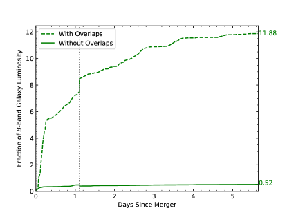
Figure 6: $B$-band Galaxy luminosity fraction observed out of all galaxies with luminosity larger than $L_{B}^{*}$ from the GLADE 2.3 catalog that are inside the 90% localization region and up to a distance of 3$\sigma$ of the mean estimated distance. The initial and updated localizations are separated by the vertical dotted grey line. The dashed line shows the total luminosity observed including overlapping galaxies, while the solid line shows the total luminosity observed in unique galaxies.

3.4 Kilonova Detection

Table 5: Parameters and distributions used for generating the ensemble of light curves from the Nicholl et al. (2021) BNS merger kilonova model.

Parameter	Description	Type	Values
$\mathcal{M}^{a}$	Chirp mass	Gaussian	$\mu=1.44$, $\sigma=0.02$
$q^{a}$	Mass ratio	uniform	$\min=0.4$, $\max=1.0$
s	Shock density profile power law index	fixed	1.0
$M_{TOV}$	NS maximum theoretical mass	fixed	2.2
$\alpha^{b}$	Enhancement of blue ejecta	uniform	$\min=0.1$, $\max=1.0$
$disk_{frac}^{b}$	Fraction of disk ejected	uniform	$\min=0.05$, $\max=0.5$
$\cos\theta^{b}$	Cosine of viewing angle	uniform	$\min=0.0$, $\max=1.0$
$\cos\theta_{cocoon}^{b}$	Cosine of cocoon opening angle	uniform	$\min=0.707$, $\max=1.0$
$\cos\theta_{open}^{b}$	Cosine of squeezed ejecta opening angle	fixed	0.707
$\log N_{H}^{b}$	Hydrogen column density	uniform	$\min=19$, $\max=23$

Even if the localization would have been covered as efficiently as possible, there is still a possibility that the EM counterpart was too faint to have been detected. In order to check this, we compare the non-detection limiting magnitudes reported for each of the followup observations to the light curve of GW170817 and to light curves generated using the Kasen et al. (2017) and Nicholl et al. (2021) kilonova models.

We use the InfraRed Survey Archive (IRSA) dust extinction service queries to correct all reported magnitude limits for Milky Way dust extinction at the center of their footprint by using the Schlafly & Finkbeiner (2011) galactic dust extinction estimates. For unfiltered observations, we assume $r$-band extinction. We then translate all limits to absolute magnitudes using the mean distance of the pixel that overlaps with the footprint center.

The GW170817 data is taken from the Arcavi (2018) compilation of observations by Andreoni et al. (2017); Arcavi et al. (2017b); Coulter et al. (2017b); Cowperthwaite et al. (2017); Díaz et al. (2017); Drout et al. (2017); Evans et al. (2017); Hu et al. (2017); Kasliwal et al. (2017); Lipunov et al. (2017); Pian et al. (2017); Shappee et al. (2017); Smartt et al. (2017); Tanvir et al. (2017); Troja et al. (2017); Utsumi et al. (2017); Valenti et al. (2017) and Pozanenko et al. (2018).

The Kasen et al. (2017) model is based on a 1D Monte Carlo simulation of the radiative transfer of photons from the radioactive decay of $r$-process elements through kilonova ejecta. The ejecta is modeled using three parameters: ejecta mass $M_{ej}$, characteristic expansion velocity $v_{k}$, and lanthanide fraction power index $X_{lan}$ (where the lanthanide fraction is $10^{X_{lan}}$). The calculation produces a spectral energy distribution of the emission. We use pyphot to create synthetic light curves in the relevant bands from these model spectra. We use the ejecta parameters assumed by Foley et al. (2020) for the GW190415 kilonova: $M_{ej}=0.04M_{\odot}$, $v_{k}=0.15c$ and $X_{lan}=-2$, which they propose assuming a BNS system with masses $1.4M_{\odot}$ and $2.0M_{\odot}$. This lanthanide fraction results in a high opacity of ${\kappa_{ej}}\approx 10\ cm^{2}/g$ and a transient that is observable mostly in the infrared. This led Foley et al. (2020) to conclude that the GW190425 kilonova would not have likely been observable to most facilities that participated in the search.

Nicholl et al. (2021) provide an analytic 2D kilonova model that assumes a three-component ejecta: one component is the “tidal ejecta” in the equatorial region and a second is the “polar ejecta” concentrated in the polar region. For both components, a blackbody is assumed. The third component is from GRB-shocked material in a “cocoon” around the polar region (Nakar & Piran, 2016). The model parameters relate directly to the GW-measured binary system chirp mass $\mathcal{M}$ and mass ratio $q$, and to neutron star (NS) equation of state parameters, such as the NS maximum theoretical mass $M_{TOV}$. These are used to calculate the mass $M_{ej}$, velocity $v_{k}$, and the opacity ${\kappa_{ej}}$ of each ejecta component corresponding to three opacity regimes: the “red” high opacity (low $Y_{e}$) tidal ejecta, the “blue” low opacity (high $Y_{e}$) polar ejecta, and the intermediate-opacity “purple” ejecta. The blue and red opacities are assumed to be $\kappa_{ej,blue}=0.5\ cm^{2}/g$ and $\kappa_{ej,red}=10\ cm^{2}/g$, respectively. The asymmetry of the ejecta is parameterized by the opening angle around the poles ${\theta_{open}}$, which separates the polar ejecta and the tidal ejecta, and the opening angle of the shocked cocoon ${\theta_{cocoon}}$. Finally, the observer’s viewing angle ${\theta}$ and the host hydrogen column density $N_{H}$ are taken as parameters as well. The model is implemented in the Modular Open Source Fitter for Transients (MOSFiT; Guillochon et al. 2018), which can be used to generate light curves in various bands. We generate an ensemble of models, using the binary parameters $\mathcal{M}$ and $q$ from Abbott et al. (2020). For the rest of the parameters, we sample 100 realizations of the ensemble from the prior distributions that Nicholl et al. (2021) used for their GW170817 kilonova fit (which included three fixed parameters, as we repeat here). The full set of parameters and the values used are described in Table 5. These parameters produce a blue kilonova ejecta component with $M_{ej,blue}=0.00154\pm 0.00036M_{\odot}$, and $v_{k,blue}=0.1513\pm 0.0024c$, a red ejecta component with $M_{ej,red}=0.0426\pm 0.0047M_{\odot}$, and $v_{k,red}=0.2586\pm 0.0024c$, and a purple ejecta component with $M_{ej,purple}=0.0235\pm 0.00036M_{\odot}$, $v_{k,purple}=0.0485\pm 0.0011c$, and $\kappa_{ej,purple}\simeq 5.6\ cm^{2}/g$. The total mass ejected of $M_{ej}=0.0676\pm 0.0045M_{\odot}$ has a mean opacity of $\kappa_{ej}=7.95\pm 0.21\ cm^{2}/g$, making the light curves bluer and more luminous overall than the Kasen et al. (2017) ones.

The comparison of reported non-detection limiting magnitudes to the GW170817 kilonova and the model light curves described above can be seen in Figure 7.

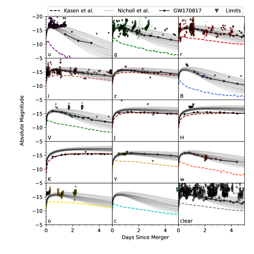
Figure 7: 5$\sigma$ non-detection limits of the GW190425 kilonova (triangles) compared to a single kilonova model from Kasen et al. (2017) (dashed lines), an ensemble of models from Nicholl et al. (2021) (semi-transparent solid grey lines; see text for details), and the GW170817 kilonova (circles; see text for data sources). The upper limit triangles are displayed fully opaque for observations within the 50% GWTC-2 localization region, partially opaque for observations outside the 50% GWTC-2 localization region but within the 90% GWTC-2 localization region, and almost transparent for observations outside the 90% GWTC-2 localization region. The limits are converted to absolute magnitude after Milky Way extinction correction and using the distance estimate at the HEALPix closest to the center of the pointing for each limit. Data in the ‘clear’ band is unfiltered and is compared to models in the $r$-band. Limits with magnitudes brighter than -20 are not shown.

We find that, had the GW190425 kilonova been similar to that of GW170817, it should have been easily detected if the entire localization region had been observed, even given the larger distance of GW190425 compared to that of GW170817. In fact, limits in the $g$- and $r$-bands are 3–4 magnitudes deeper than what would have been required to observe a GW170817-like kilonova at peak. However, given the different merger parameters, it is not clear whether the GW190425 kilonova would have been as luminous as that of GW170817. Indeed, the Kasen et al. (2017) models predict much fainter optical emission. According to that model, the kilonova would just have barely been detected in a few of the bands used in the search. The Nicholl et al. (2021) models, on the other hand, predict a kilonova that would have been detected easily in the optical bands as well. The two model predictions differ by as much as $6$ magnitudes in the optical bands.

4 Summary and Conclusions

We analyzed all reported ultraviolet, optical and infrared followup observations of GW190425, the only robust BNS merger detected since GW170817, and showed that:

1. Other than some sun and moon constrained regions, most of the localization region of GW190425 was observable at the time of the trigger.

2. Enough observational resources were invested in the followup of GW190425 to allow the accessible part of the 90% probability region to have been covered potentially in a few hours. Instead, several regions were observed over 100 times, while others were never observed, and more than 5 days after the merger, only 50% of the probability was covered.

3. Even if the GW190425 kilonova were 3–4 magnitudes fainter than the GW170817 kilonova in its optical peak, it could still have been detected. According to more conservative models without a blue emission component, the kilonova might have been only marginally detected around peak.

These results only take into account observations undertaken by facilities which decided to followup GW190425. It is not possible to know which additional facilities prefered not to trigger given the large localization region, but which might have participated in the search, had they known that roughly half of the probability was already being covered by others.

We conclude that even for relatively distant BNS mergers with large localizations, coordinated followup can significantly increase the chances of discovering an EM counterpart. The lack of coordination during the followup of GW190425 strongly contributed to the failure to identify its EM counterpart. In addition, lack of coordination weakens our ability to constrain models of kilonova emission, given the amount of localization probability that was not covered, and for which no limits are available. Even for smaller localiztions, coordination can help find the kilonova sooner. Observations on few-hour time scales are critical for constraining emission models (e.g. Arcavi, 2018).

Real-time coordination in such a competitive field, requiring very rapid response, is challenging. Tools like the Treasure Map have been built exactly to overcome this challenge. We encourage the community to report their pointings to the Treasure Map, and to use the information there to guide their search, even if it means searching lower probability areas (instead of contributing the 100th observation to a higher probability region).

With the lack of additional significant BNS merger discoveries since GW190425, it is possible that the BNS merger rate is on the lower end of its large uncertainty range, and events as nearby and well localized as GW170817 are likely very rare. If we wish to unleash the potential of GW-EM multi-messenger astronomy for nuclear physics, astrophysics, and cosmology, we must better coordinate our GW followup searches.

Appendix A Healpy Exclusive vs. Inclusive Methods

We present an illustration of the inclusive vs. the exclusive methods of healpy pixel queries in Figure 8. The inclusive method can significantly overestimate the area covered by a footprint with a field of view smaller than the pixel size. The exclusive method is much more conservative, and hence we chose it for our analysis.

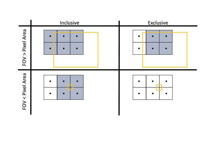
Figure 8: An illustration of the exclusive and inclusive healpy pixel query methods. Each black square represents a pixel centered around a black dot and the yellow rectangles are hypothetical observational footprints. Grey pixels are the ones returned according to each method and white pixels are ignored. The inclusive method (left) returns every pixel that intersects with the observed footprint, while the exclusive method (right) returns only pixels with centers included in the observed footprint. For footprints with a field of view (FOV) much smaller than the pixel area (bottom), the inclusive method can significantly overestimate the area covered.

References

- Abbott et al. (2017a) Abbott, B. P., Abbott, R., Abbott, T. D., et al. 2017a, Phys. Rev. Lett., 119, 161101, doi: 10.1103/PhysRevLett.119.161101
- Abbott et al. (2017b) —. 2017b, ApJ, 848, L13, doi: 10.3847/2041-8213/aa920c
- Abbott et al. (2017) Abbott, B. P., Abbott, R., Abbott, T. D., et al. 2017, The Astrophysical Journal Letters, 848, L12, doi: 10.3847/2041-8213/aa91c9
- Abbott et al. (2017) Abbott, B. P., Abbott, R., Abbott, T. D., et al. 2017, Nature, 551, 85, doi: 10.1038/nature24471
- Abbott et al. (2020) Abbott, B. P., Abbott, R., Abbott, T. D., et al. 2020, The Astrophysical Journal Letters, 892, L3, doi: 10.3847/2041-8213/ab75f5
- Abbott et al. (2021) Abbott, R., Abbott, T. D., Abraham, S., & et al. 2021, Physical Review X, 11, 021053, doi: 10.1103/PhysRevX.11.021053
- Acernese et al. (2014) Acernese, F., Agathos, M., Agatsuma, K., et al. 2014, Classical and Quantum Gravity, 32, 024001, doi: 10.1088/0264-9381/32/2/024001
- Ahumada et al. (2019a) Ahumada, T., Coughlin, M. W., Staats, K., Burdge, K., & Dekany, R. G. 2019a, GRB Coordinates Network, 24320, 1
- Ahumada et al. (2019b) Ahumada, T., Coughlin, M. W., Staats, K., & Dekany, R. G. 2019b, GRB Coordinates Network, 24198, 1
- Ahumada et al. (2019c) Ahumada, T., Coughlin, M. W., Staats, K., et al. 2019c, GRB Coordinates Network, 24343, 1
- Andreoni et al. (2017) Andreoni, I., Ackley, K., Cooke, J., et al. 2017, PASA, 34, e069, doi: 10.1017/pasa.2017.65
- Antier et al. (2020) Antier, S., Agayeva, S., Aivazyan, V., et al. 2020, MNRAS, 492, 3904, doi: 10.1093/mnras/stz3142
- Arcavi (2018) Arcavi, I. 2018, The Astrophysical Journal Letters, 855, L23, doi: 10.3847/2041-8213/aab267
- Arcavi et al. (2019) Arcavi, I., Howell, D. A., McCully, C., et al. 2019, GRB Coordinates Network, 24307, 1
- Arcavi et al. (2017a) Arcavi, I., McCully, C., Hosseinzadeh, G., et al. 2017a, ApJ, 848, L33, doi: 10.3847/2041-8213/aa910f
- Arcavi et al. (2017b) Arcavi, I., Hosseinzadeh, G., Howell, D. A., et al. 2017b, Nature, 551, 64, doi: 10.1038/nature24291
- Astropy Collaboration et al. (2022) Astropy Collaboration, Price-Whelan, A. M., Lim, P. L., et al. 2022, ApJ, 935, 167, doi: 10.3847/1538-4357/ac7c74
- Atwood et al. (2009) Atwood, W. B., Abdo, A. A., Ackermann, M., et al. 2009, ApJ, 697, 1071, doi: 10.1088/0004-637X/697/2/1071
- Axelsson et al. (2019) Axelsson, M., Omodei, N., Kocevski, D., & Longo, F. 2019, GRB Coordinates Network, 24174, 1
- Barnes & Kasen (2013) Barnes, J., & Kasen, D. 2013, The Astrophysical Journal, 775, 18, doi: 10.1088/0004-637X/775/1/18
- Bauswein et al. (2013) Bauswein, A., Goriely, S., & Janka, H. T. 2013, ApJ, 773, 78, doi: 10.1088/0004-637X/773/1/78
- Bhalerao et al. (2019) Bhalerao, V., Kumar, H., Karambelkar, V., et al. 2019, GRB Coordinates Network, 24201, 1
- Blazek et al. (2019) Blazek, M., Christensen, N., Howell, E., et al. 2019, GRB Coordinates Network, 24227, 1
- Bloom et al. (2019) Bloom, J. S., Zucker, C., Schlafly, E., et al. 2019, GRB Coordinates Network, 24337, 1
- Boër et al. (1999) Boër, M., Bringer, M., Klotz, A., et al. 1999, A&AS, 138, 579, doi: 10.1051/aas:1999356
- Bowen & Vaughan (1973) Bowen, I. S., & Vaughan, A. H., J. 1973, Appl. Opt., 12, 1430, doi: 10.1364/AO.12.001430
- Brown et al. (2013) Brown, T. M., Baliber, N., Bianco, F. B., et al. 2013, PASP, 125, 1031, doi: 10.1086/673168
- Burke et al. (2019) Burke, J., Hiramatsu, D., Arcavi, I., et al. 2019, GRB Coordinates Network, 24206, 1
- Butler et al. (2019) Butler, N., Watson, A. M., Troja, E., et al. 2019, GRB Coordinates Network, 24238, 1
- Camilletti et al. (2022) Camilletti, A., Chiesa, L., Ricigliano, G., et al. 2022, Monthly Notices of the Royal Astronomical Society, 516, 4760, doi: 10.1093/mnras/stac2333
- Castro-Tirado et al. (2019) Castro-Tirado, A. J., Hu, Y. D., Li, X. Y., et al. 2019, GRB Coordinates Network, 24214, 1
- Chambers et al. (2016) Chambers, K. C., Magnier, E. A., Metcalfe, N., et al. 2016, arXiv e-prints, arXiv:1612.05560, doi: 10.48550/arXiv.1612.05560
- Chang et al. (2019) Chang, S. W., Wolf, C., Onken, C. A., Luvaul, L., & Scott, S. 2019, GRB Coordinates Network, 24325, 1
- Clark & Eardley (1977) Clark, J. P. A., & Eardley, D. M. 1977, ApJ, 215, 311, doi: 10.1086/155360
- Cobos et al. (2002) Cobos, F. J., Gonzalez, J. J., Tejada, C., Cepa, J., & Rasilla, J. L. 2002, in Society of Photo-Optical Instrumentation Engineers (SPIE) Conference Series, Vol. 4832, Society of Photo-Optical Instrumentation Engineers (SPIE) Conference Series, 249–257, doi: 10.1117/12.486467
- Coulter et al. (2017a) Coulter, D. A., Kilpatrick, C. D., Siebert, M. R., et al. 2017a, GRB Coordinates Network, 21529, 1
- Coulter et al. (2017b) Coulter, D. A., Foley, R. J., Kilpatrick, C. D., et al. 2017b, Science, 358, 1556, doi: 10.1126/science.aap9811
- Coulter et al. (2024) Coulter, D. A., Kilpatrick, C. D., Jones, D. O., et al. 2024, arXiv e-prints, arXiv:2404.15441, doi: 10.48550/arXiv.2404.15441
- Cowperthwaite et al. (2017) Cowperthwaite, P. S., Berger, E., Villar, V. A., et al. 2017, ApJ, 848, L17, doi: 10.3847/2041-8213/aa8fc7
- Dalton et al. (2006) Dalton, G. B., Caldwell, M., Ward, A. K., et al. 2006, in Society of Photo-Optical Instrumentation Engineers (SPIE) Conference Series, Vol. 6269, Society of Photo-Optical Instrumentation Engineers (SPIE) Conference Series, ed. I. S. McLean & M. Iye, 62690X, doi: 10.1117/12.670018
- Dálya et al. (2018) Dálya, G., Galgóczi, G., Dobos, L., et al. 2018, MNRAS, 479, 2374, doi: 10.1093/mnras/sty1703
- DePoy et al. (2003) DePoy, D. L., Atwood, B., Belville, S. R., et al. 2003, in Society of Photo-Optical Instrumentation Engineers (SPIE) Conference Series, Vol. 4841, Instrument Design and Performance for Optical/Infrared Ground-based Telescopes, ed. M. Iye & A. F. M. Moorwood, 827–838, doi: 10.1117/12.459907
- Díaz et al. (2017) Díaz, M. C., Macri, L. M., Garcia Lambas, D., et al. 2017, ApJ, 848, L29, doi: 10.3847/2041-8213/aa9060
- Djupvik & Andersen (2010) Djupvik, A. A., & Andersen, J. 2010, in Astrophysics and Space Science Proceedings, Vol. 14, Highlights of Spanish Astrophysics V, 211, doi: 10.1007/978-3-642-11250-8_21
- Drake et al. (2009) Drake, A. J., Djorgovski, S. G., Mahabal, A., et al. 2009, ApJ, 696, 870, doi: 10.1088/0004-637X/696/1/870
- Drout et al. (2017) Drout, M. R., Piro, A. L., Shappee, B. J., et al. 2017, Science, 358, 1570, doi: 10.1126/science.aaq0049
- Dudi et al. (2022) Dudi, R., Adhikari, A., Brügmann, B., et al. 2022, Phys. Rev. D, 106, 084039, doi: 10.1103/PhysRevD.106.084039
- Dyer et al. (2022) Dyer, M. J., Ackley, K., Lyman, J., et al. 2022, in Society of Photo-Optical Instrumentation Engineers (SPIE) Conference Series, Vol. 12182, Ground-based and Airborne Telescopes IX, ed. H. K. Marshall, J. Spyromilio, & T. Usuda, 121821Y, doi: 10.1117/12.2629369
- Eichler et al. (1989) Eichler, D., Livio, M., Piran, T., & Schramm, D. N. 1989, Nature, 340, 126, doi: 10.1038/340126a0
- Emerson et al. (2006) Emerson, J., McPherson, A., & Sutherland, W. 2006, The Messenger, 126, 41
- Evans et al. (2017) Evans, P. A., Cenko, S. B., Kennea, J. A., et al. 2017, Science, 358, 1565, doi: 10.1126/science.aap9580
- Fabricant et al. (2019) Fabricant, D., Fata, R., Epps, H., et al. 2019, PASP, 131, 075004, doi: 10.1088/1538-3873/ab1d78
- Farah et al. (2010) Farah, A., Barojas, E., Butler, N. R., et al. 2010, in Society of Photo-Optical Instrumentation Engineers (SPIE) Conference Series, Vol. 7735, Ground-based and Airborne Instrumentation for Astronomy III, ed. I. S. McLean, S. K. Ramsay, & H. Takami, 77357Z, doi: 10.1117/12.857828
- Filippenko et al. (2001) Filippenko, A. V., Li, W. D., Treffers, R. R., & Modjaz, M. 2001, in Astronomical Society of the Pacific Conference Series, Vol. 246, IAU Colloq. 183: Small Telescope Astronomy on Global Scales, ed. B. Paczynski, W.-P. Chen, & C. Lemme, 121
- Flaugher et al. (2015) Flaugher, B., Diehl, H. T., Honscheid, K., et al. 2015, AJ, 150, 150, doi: 10.1088/0004-6256/150/5/150
- Fletcher et al. (2019) Fletcher, C., Fermi-GBM Team, & GBM-LIGO/Virgo Group. 2019, GRB Coordinates Network, 24185, 1
- Foley et al. (2020) Foley, R. J., Coulter, D. A., Kilpatrick, C. D., et al. 2020, Monthly Notices of the Royal Astronomical Society, 494, 190, doi: 10.1093/mnras/staa725
- Foley et al. (2020) Foley, R. J., Coulter, D. A., Kilpatrick, C. D., et al. 2020, MNRAS, 494, 190, doi: 10.1093/mnras/staa725
- Gehrels et al. (2004) Gehrels, N., Chincarini, G., Giommi, P., et al. 2004, ApJ, 611, 1005, doi: 10.1086/422091
- Gompertz et al. (2020) Gompertz, B. P., Cutter, R., Steeghs, D., et al. 2020, MNRAS, 497, 726, doi: 10.1093/mnras/staa1845
- Górski et al. (2005) Górski, K. M., Hivon, E., Banday, A. J., et al. 2005, ApJ, 622, 759, doi: 10.1086/427976
- Greiner et al. (2008) Greiner, J., Bornemann, W., Clemens, C., et al. 2008, PASP, 120, 405, doi: 10.1086/587032
- Grossman et al. (2014) Grossman, D., Korobkin, O., Rosswog, S., & Piran, T. 2014, Monthly Notices of the Royal Astronomical Society, 439, 757, doi: 10.1093/mnras/stt2503
- Guillochon et al. (2018) Guillochon, J., Nicholl, M., Villar, V. A., et al. 2018, ApJS, 236, 6, doi: 10.3847/1538-4365/aab761
- Guo et al. (2022) Guo, B., Peng, Q., Chen, Y., et al. 2022, Research in Astronomy and Astrophysics, 22, 055007, doi: 10.1088/1674-4527/ac5959
- Han et al. (2005) Han, W., Mack, P., Lee, C.-U., et al. 2005, PASJ, 57, 821, doi: 10.1093/pasj/57.5.821
- Han et al. (2021) Han, X., Xiao, Y., Zhang, P., et al. 2021, Publications of the Astronomical Society of the Pacific, 133, 065001, doi: 10.1088/1538-3873/abfb4e
- Hiramatsu et al. (2019a) Hiramatsu, D., Arcavi, I., Burke, J., et al. 2019a, GRB Coordinates Network, 24194, 1
- Hiramatsu et al. (2019b) Hiramatsu, D., Pellegrino, C., Burke, J., et al. 2019b, GRB Coordinates Network, 24225, 1
- Hosseinzadeh et al. (2019a) Hosseinzadeh, G., Cowperthwaite, P. S., Gomez, S., et al. 2019a, ApJ, 880, L4, doi: 10.3847/2041-8213/ab271c
- Hosseinzadeh et al. (2019b) Hosseinzadeh, G., Berger, E., Blanchard, P. K., et al. 2019b, GRB Coordinates Network, 24182, 1
- Hotokezaka et al. (2013) Hotokezaka, K., Kiuchi, K., Kyutoku, K., et al. 2013, Phys. Rev. D, 87, 024001, doi: 10.1103/PhysRevD.87.024001
- Howell et al. (2019) Howell, E., Christensen, N., Blazek, M., et al. 2019, GRB Coordinates Network, 24256, 1
- Hu et al. (2017) Hu, L., Wu, X., Andreoni, I., et al. 2017, Science Bulletin, 62, 1433, doi: 10.1016/j.scib.2017.10.006
- Hu et al. (2019a) Hu, Y. D., Li, X. Y., Carrasco, I., et al. 2019a, GRB Coordinates Network, 24270, 1
- Hu et al. (2019b) Hu, Y. D., Castro-Tirado, A. J., Li, X. Y., et al. 2019b, GRB Coordinates Network, 24324, 1
- Hunter (2007) Hunter, J. D. 2007, Computing in Science and Engineering, 9, 90, doi: 10.1109/MCSE.2007.55
- Im et al. (2019) Im, M., Paek, G. S. H., Lim, G., et al. 2019, GRB Coordinates Network, 24183, 1
- Izzo et al. (2019) Izzo, L., Malesani, D. B., & Carini, R. 2019, GRB Coordinates Network, 24319, 1
- Kann et al. (2019) Kann, D. A., Thoene, C., Stachie, C., et al. 2019, GRB Coordinates Network, 24459, 1
- Kasen et al. (2013) Kasen, D., Badnell, N. R., & Barnes, J. 2013, The Astrophysical Journal, 774, 25, doi: 10.1088/0004-637X/774/1/25
- Kasen et al. (2017) Kasen, D., Metzger, B., Barnes, J., Quataert, E., & Ramirez-Ruiz, E. 2017, Nature, 551, 80, doi: 10.1038/nature24453
- Kashikawa et al. (2002) Kashikawa, N., Aoki, K., Asai, R., et al. 2002, PASJ, 54, 819, doi: 10.1093/pasj/54.6.819
- Kasliwal et al. (2017) Kasliwal, M. M., Nakar, E., Singer, L. P., et al. 2017, Science, 358, 1559, doi: 10.1126/science.aap9455
- Kasliwal et al. (2019) Kasliwal, M. M., Cannella, C., Bagdasaryan, A., et al. 2019, PASP, 131, 038003, doi: 10.1088/1538-3873/aafbc2
- Keller et al. (2007) Keller, S. C., Schmidt, B. P., Bessell, M. S., et al. 2007, PASA, 24, 1, doi: 10.1071/AS07001
- Kim et al. (2019) Kim, J., Im, M., Lee, C. U., et al. 2019, GRB Coordinates Network, 24216, 1
- Kim et al. (2016) Kim, S.-L., Lee, C.-U., Park, B.-G., et al. 2016, Journal of Korean Astronomical Society, 49, 37, doi: 10.5303/JKAS.2016.49.1.37
- Kong (2019) Kong, A. 2019, GRB Coordinates Network, 24303, 1
- Kulkarni (2005) Kulkarni, S. R. 2005, arXiv e-prints, astro, doi: 10.48550/arXiv.astro-ph/0510256
- Kyutoku et al. (2020) Kyutoku, K., Fujibayashi, S., Hayashi, K., et al. 2020, ApJ, 890, L4, doi: 10.3847/2041-8213/ab6e70
- Li et al. (2019a) Li, B., Xu, D., Zhou, X., & Lu, H. 2019a, GRB Coordinates Network, 24285, 1
- Li & Paczyński (1998) Li, L.-X., & Paczyński, B. 1998, The Astrophysical Journal, 507, L59, doi: 10.1086/311680
- Li et al. (2019b) Li, W. X., Chen, J. C., Xiaofeng, W. X., et al. 2019b, GRB Coordinates Network, 24267, 1
- Ligo Scientific Collaboration & VIRGO Collaboration (2019a) Ligo Scientific Collaboration, & VIRGO Collaboration. 2019a, GRB Coordinates Network, 24168, 1
- Ligo Scientific Collaboration & VIRGO Collaboration (2019b) —. 2019b, GRB Coordinates Network, 24228, 1
- LIGO Scientific Collaboration et al. (2015) LIGO Scientific Collaboration, T., Aasi, J., Abbott, B. P., et al. 2015, Classical and Quantum Gravity, 32, 074001, doi: 10.1088/0264-9381/32/7/074001
- Lipunov et al. (2010) Lipunov, V., Kornilov, V., Gorbovskoy, E., et al. 2010, Advances in Astronomy, 2010, 349171, doi: 10.1155/2010/349171
- Lipunov et al. (2017) Lipunov, V. M., Gorbovskoy, E., Kornilov, V. G., et al. 2017, ApJ, 850, L1, doi: 10.3847/2041-8213/aa92c0
- Lundquist et al. (2019) Lundquist, M. J., Paterson, K., Fong, W., et al. 2019, ApJ, 881, L26, doi: 10.3847/2041-8213/ab32f2
- Margutti & Chornock (2021) Margutti, R., & Chornock, R. 2021, ARA&A, 59, 155, doi: 10.1146/annurev-astro-112420-030742
- Masci et al. (2018) Masci, F. J., Laher, R. R., Rusholme, B., et al. 2018, Publications of the Astronomical Society of the Pacific, 131, 018003, doi: 10.1088/1538-3873/aae8ac
- Meegan et al. (2009) Meegan, C., Lichti, G., Bhat, P. N., et al. 2009, The Astrophysical Journal, 702, 791, doi: 10.1088/0004-637X/702/1/791
- Metzger et al. (2010) Metzger, B. D., Martínez-Pinedo, G., Darbha, S., et al. 2010, Monthly Notices of the Royal Astronomical Society, 406, 2650, doi: 10.1111/j.1365-2966.2010.16864.x
- Morihana et al. (2019a) Morihana, K., Jian, M., & Nagayama, T. 2019a, GRB Coordinates Network, 24219, 1
- Morihana et al. (2019b) —. 2019b, GRB Coordinates Network, 24328, 1
- Nagayama et al. (2003) Nagayama, T., Nagashima, C., Nakajima, Y., et al. 2003, in Society of Photo-Optical Instrumentation Engineers (SPIE) Conference Series, Vol. 4841, Instrument Design and Performance for Optical/Infrared Ground-based Telescopes, ed. M. Iye & A. F. M. Moorwood, 459–464, doi: 10.1117/12.460770
- Nakar (2020) Nakar, E. 2020, Phys. Rep., 886, 1, doi: 10.1016/j.physrep.2020.08.008
- Nakar & Piran (2016) Nakar, E., & Piran, T. 2016, The Astrophysical Journal, 834, 28, doi: 10.3847/1538-4357/834/1/28
- Nicholl et al. (2021) Nicholl, M., Margalit, B., Schmidt, P., et al. 2021, MNRAS, 505, 3016, doi: 10.1093/mnras/stab1523
- Nicholl et al. (2021) Nicholl, M., Margalit, B., Schmidt, P., et al. 2021, Monthly Notices of the Royal Astronomical Society, 505, 3016, doi: 10.1093/mnras/stab1523
- Paek et al. (2019) Paek, G. S. H., Im, M., Lim, G., et al. 2019, GRB Coordinates Network, 24188, 1
- Park et al. (2012) Park, W.-K., Pak, S., Im, M., et al. 2012, PASP, 124, 839, doi: 10.1086/667390
- Perley & Copperwheat (2019) Perley, D. A., & Copperwheat, C. M. 2019, GRB Coordinates Network, 24202, 1
- Perley et al. (2019) Perley, D. A., Copperwheat, C. M., & Taggart, K. L. 2019, GRB Coordinates Network, 24314, 1
- Pian et al. (2017) Pian, E., D’Avanzo, P., Benetti, S., et al. 2017, Nature, 551, 67, doi: 10.1038/nature24298
- Piro & Kollmeier (2018) Piro, A. L., & Kollmeier, J. A. 2018, ApJ, 855, 103, doi: 10.3847/1538-4357/aaaab3
- Pozanenko et al. (2020) Pozanenko, A. S., Minaev, P. Y., Grebenev, S. A., & Chelovekov, I. V. 2020, Astronomy Letters, 45, 710, doi: 10.1134/S1063773719110057
- Pozanenko et al. (2018) Pozanenko, A. S., Barkov, M. V., Minaev, P. Y., et al. 2018, ApJ, 852, L30, doi: 10.3847/2041-8213/aaa2f6
- Radice et al. (2024) Radice, D., Ricigliano, G., Bhattacharya, M., et al. 2024, Monthly Notices of the Royal Astronomical Society, 528, 5836, doi: 10.1093/mnras/stae400
- Roming et al. (2005) Roming, P. W. A., Kennedy, T. E., Mason, K. O., et al. 2005, Space Sci. Rev., 120, 95, doi: 10.1007/s11214-005-5095-4
- Rosswog et al. (1999) Rosswog, S., Liebendörfer, M., Thielemann, F. K., et al. 1999, A&A, 341, 499, doi: 10.48550/arXiv.astro-ph/9811367
- Sagués Carracedo et al. (2021) Sagués Carracedo, A., Bulla, M., Feindt, U., & Goobar, A. 2021, MNRAS, 504, 1294, doi: 10.1093/mnras/stab872
- Sakamoto et al. (2019) Sakamoto, T., Barthelmy, S. D., Lien, A. Y., et al. 2019, GRB Coordinates Network, 24184, 1
- Sasada et al. (2019) Sasada, M., Akitaya, H., Nakaoka, T., et al. 2019, GRB Coordinates Network, 24192, 1
- Savchenko et al. (2019) Savchenko, V., Ferrigno, C., Martin-Carillo, A., et al. 2019, GRB Coordinates Network, 24178, 1
- Schady et al. (2019) Schady, P., Chen, T. W., Schweyer, T., Malesani, D. B., & Bolmer, J. 2019, GRB Coordinates Network, 24229, 1
- Schechter (1976) Schechter, P. 1976, ApJ, 203, 297, doi: 10.1086/154079
- Schlafly & Finkbeiner (2011) Schlafly, E. F., & Finkbeiner, D. P. 2011, ApJ, 737, 103, doi: 10.1088/0004-637X/737/2/103
- Shappee et al. (2017) Shappee, B. J., Simon, J. D., Drout, M. R., et al. 2017, Science, 358, 1574, doi: 10.1126/science.aaq0186
- Smartt et al. (2017) Smartt, S. J., Chen, T. W., Jerkstrand, A., et al. 2017, Nature, 551, 75, doi: 10.1038/nature24303
- Smartt et al. (2024) Smartt, S. J., Nicholl, M., Srivastav, S., et al. 2024, MNRAS, 528, 2299, doi: 10.1093/mnras/stae100
- Steele et al. (2004) Steele, I. A., Smith, R. J., Rees, P. C., et al. 2004, in Society of Photo-Optical Instrumentation Engineers (SPIE) Conference Series, Vol. 5489, Ground-based Telescopes, ed. J. Oschmann, Jacobus M., 679–692, doi: 10.1117/12.551456
- Sun et al. (2019) Sun, T., Chen, J., Hu, L., et al. 2019, GRB Coordinates Network, 24234, 1
- Swift et al. (2022) Swift, J. J., Andersen, K., Arculli, T., et al. 2022, Publications of the Astronomical Society of the Pacific, 134, 035005, doi: 10.1088/1538-3873/ac5aca
- Tan et al. (2019a) Tan, H. J., Yu, P. C., Ngeow, C. C., & Ip, W. H. 2019a, GRB Coordinates Network, 24193, 1
- Tan et al. (2019b) Tan, H. J., Yu, P. C., Patil, A. S., et al. 2019b, GRB Coordinates Network, 24274, 1
- Tanaka & Hotokezaka (2013) Tanaka, M., & Hotokezaka, K. 2013, The Astrophysical Journal, 775, 113, doi: 10.1088/0004-637X/775/2/113
- Tanvir et al. (2019) Tanvir, N. R., Gonzalez-Fernandez, C., Levan, A. J., Malesani, D. B., & Evans, P. A. 2019, GRB Coordinates Network, 24334, 1
- Tanvir et al. (2017) Tanvir, N. R., Levan, A. J., González-Fernández, C., et al. 2017, ApJ, 848, L27, doi: 10.3847/2041-8213/aa90b6
- Tonry et al. (2018) Tonry, J. L., Denneau, L., Heinze, A. N., et al. 2018, PASP, 130, 064505, doi: 10.1088/1538-3873/aabadf
- Troja et al. (2017) Troja, E., Piro, L., van Eerten, H., et al. 2017, Nature, 551, 71, doi: 10.1038/nature24290
- Troja et al. (2019) Troja, E., Watson, A. M., Becerra, R. L., et al. 2019, GRB Coordinates Network, 24335, 1
- Utsumi et al. (2017) Utsumi, Y., Tanaka, M., Tominaga, N., et al. 2017, PASJ, 69, 101, doi: 10.1093/pasj/psx118
- Valenti et al. (2017) Valenti, S., Sand, D. J., Yang, S., et al. 2017, ApJ, 848, L24, doi: 10.3847/2041-8213/aa8edf
- van der Walt et al. (2011) van der Walt, S., Colbert, S. C., & Varoquaux, G. 2011, Computing in Science and Engineering, 13, 22, doi: 10.1109/MCSE.2011.37
- Vinko et al. (2019) Vinko, A., Bodi, L., Kriskovics, K., Sarneczky, K., & Pal, A. 2019, GRB Coordinates Network, 24367, 1
- Wang et al. (2019) Wang, C.-J., Bai, J.-M., Fan, Y.-F., et al. 2019, Research in Astronomy and Astrophysics, 19, 149, doi: 10.1088/1674-4527/19/10/149
- Waratkar et al. (2019) Waratkar, G., Kumar, H., Bhalerao, V., Stanzin, J., & Anupama, G. C. 2019, GRB Coordinates Network, 24304, 1
- Watson et al. (2016) Watson, A. M., Cuevas Cardona, S., Alvarez Nuñez, L. C., et al. 2016, in Society of Photo-Optical Instrumentation Engineers (SPIE) Conference Series, Vol. 9908, Ground-based and Airborne Instrumentation for Astronomy VI, ed. C. J. Evans, L. Simard, & H. Takami, 99085O, doi: 10.1117/12.2233000
- Watson et al. (2019) Watson, A. M., Butler, N., Troja, E., et al. 2019, GRB Coordinates Network, 24239, 1
- Waxman et al. (2018) Waxman, E., Ofek, E. O., Kushnir, D., & Gal-Yam, A. 2018, MNRAS, 481, 3423, doi: 10.1093/mnras/sty2441
- Wenger et al. (2000) Wenger, M., Ochsenbein, F., Egret, D., et al. 2000, A&AS, 143, 9, doi: 10.1051/aas:2000332
- Winkler et al. (2003) Winkler, C., Courvoisier, T. J. L., Di Cocco, G., et al. 2003, A&A, 411, L1, doi: 10.1051/0004-6361:20031288
- Wyatt et al. (2020) Wyatt, S. D., Tohuvavohu, A., Arcavi, I., et al. 2020, ApJ, 894, 127, doi: 10.3847/1538-4357/ab855e
- Xin et al. (2019) Xin, L. P., Han, X. H., Wei, J. Y., et al. 2019, GRB Coordinates Network, 24315, 1
- Xu et al. (2019) Xu, D., Zhu, Z. P., Yu, B. Y., et al. 2019, GRB Coordinates Network, 24190, 1
- Yoshida et al. (2000) Yoshida, M., Shimizu, Y., Sasaki, T., et al. 2000, in Society of Photo-Optical Instrumentation Engineers (SPIE) Conference Series, Vol. 4009, Advanced Telescope and Instrumentation Control Software, ed. H. Lewis, 240–249, doi: 10.1117/12.388394
- Zheng et al. (2019) Zheng, W., Zhang, K., Vasylyev, S., & Filippenko, A. V. 2019, GRB Coordinates Network, 24179, 1