ROSE: Register Assisted General Time Series Forecasting with Decomposed Frequency Learning

Abstract

With the increasing collection of time series data from various domains, there arises a strong demand for general time series forecasting models pre-trained on a large number of time-series datasets to support a variety of downstream prediction tasks. Enabling general time series forecasting faces two challenges: how to obtain unified representations from multi-domian time series data, and how to capture domain-specific features from time series data across various domains for adaptive transfer in downstream tasks. To address these challenges, we propose a Register Assisted General Time Series Forecasting Model with Decomposed Frequency Learning (ROSE), a novel pre-trained model for time series forecasting. ROSE employs Decomposed Frequency Learning for the pre-training task, which decomposes coupled semantic and periodic information in time series with frequency-based masking and reconstruction to obtain unified representations across domains. We also equip ROSE with a Time Series Register, which learns to generate a register codebook to capture domain-specific representations during pre-training and enhances domain-adaptive transfer by selecting related register tokens on downstream tasks. After pre-training on large-scale time series data, ROSE achieves state-of-the-art forecasting performance on 8 real-world benchmarks. Remarkably, even in few-shot scenarios, it demonstrates competitive or superior performance compared to existing methods trained with full data.

1 Introduction

Time Series Forecasting plays a pivotal role across numerous domains, such as energy, smart transportation, weather, and economics [1]. However, training specific models in deep learning for each dataset is costly and requires tailored parameter tuning, whose prediction accuracy may be limited due to data scarcity [2]. One solution is to pre-train a general model on diverse time series datasets and fine-tune it with a few data for different downstream scenarios. However, applying this paradigm to heterogeneous time series data presents challenges.

Obtaining a unified representation from time series data across various domains is challenging. Time series from each domain involve complex temporal patterns, composed of multiple frequency components combined with each other [3], which is frequency superposition. As shown in Figure 1(a), different frequency components contain distinct semantic information. For example, low and high-frequency components represent long-term trends and rapid variations, respectively [4]. Additionally, different frequency components also contain cross-period information, revealing the interactions between short and long-term patterns in the time series. Thus, the frequency superposition leads to coupled semantic and periodic information in the time domain. Furthermore, large-scale time series data from different domains introduce even more complex temporal patterns and frequency diversity. Existing pre-training frameworks [5, 6, 7], such as mask modeling and contrastive learning, were proposed to learn a unified representation from time series data. However, these methods overlook the frequency diversity and complexity exhibited in heterogeneous time series that come from various domains, making it difficult to capture intricate patterns, thus limiting their generalization capabilities.

Adaptive transferring information from multi-domain time series to specific downstream scenarios presents a challenge. Multi-source time series data originate from various domains [8], whose data exhibit domain-specific information [2]. Information from the same or similar domain as the target domain is useful for improving the model’s effectiveness in the target task [9]. However, as shown in Figure 1(a), existing time series pre-training frameworks [8, 2, 10] focus mainly on capturing generalized features during pre-training and overlook domain-specific features. Thus, they only transfer the same generalized representation to different target domains, called direct transfer, which limits the model’s effectiveness in specific downstream tasks, as shown in Figure 1(b). Therefore, it is necessary to learn domain-specific information during pre-training and adaptively transfer the specific representations to each target domain, called adaptive transfer. Realizing adaptive transfer poses two difficulties: 1) capturing domain-specific information in pre-training. 2) adaptive use of domain-specific information in various downstream tasks.

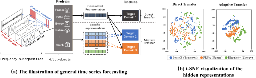
Figure 1: (a) Pre-training on multi-domain datasets that exhibit combined frequency. Existing general time series forecasting models only extract generalized representations for direct transfer to various downstream target domains. We propose to learn generalized and specific representations during pre-training, and adaptively transfer them to each target domain. (b) The t-SNE visualization of the hidden representations after direct transfer and adaptive transfer: In direct transfer, representations of different domains are mixed, but in adaptive transfer, they show a clear clustering pattern.

To address these challenges, we propose a register assisted general time series forecasting model with decomposed frequency learning (ROSE). First, we propose Decomposed Frequency Learning that learns generalized representations to solve the issue with coupled semantic and periodic information. We decompose individual time series using the Fourier transform with a novel frequency-based mask method, and then convert it back to the time domain to obtain decoupled time series for reconstruction. It makes complex temporal patterns disentangled, thus benefiting the model to learn generalized representations. Second, we introduce Time Series Register (TS-Register) to learn domain-specific information in multi-domain data. By setting up a register codebook, we generate register tokens to learn each domain-specific information during pre-training. In a downstream scenario, the model adaptively selects vectors from the register codebook that are close to the target domain of interest. During fine-tuning, we incorporate learnable vectors into the selected register tokens to complement target specific information to perform more flexible adaptive transfer. As shown in Figure 1(b), adaptive transfer successfully utilizes domain-specific information in multi-domain time series, which contributes to the model’s performance in target tasks. The contributions are summarized as follows:

• We propose ROSE, a novel general time series forecasting model using multi-domain datasets for pre-training and improving downstream fine-tuning performance and efficiency.

• We propose a novel Decomposed Frequency Learning that employs multi-frequency masking to decouple complex temporal patterns, empowering the model’s generalization capability.

• We propose TS-Register to capture domain-specific information in pre-training and enable adaptive transfer of target-oriented specific information for downstream tasks in fine-tuning.

• Our experiments with 8 real-world benchmarks demonstrate that ROSE achieves state-of-the-art performance in full-shot setting and achieves competitive or superior results in few-shot setting, along with impressive transferability in zero-shot setting.

2 Related work

2.1 Time series forecasting

Traditional time series prediction models like ARIMA [11], despite their theoretical support, are limited in modeling nonlinearity. With the rise of deep learning, many RNN-based models [12, 13, 14] have been proposed, modeling the sequential data with an autoregressive process. CNN-based models [15, 16] have also received widespread attention due to their ability to capture local features. MICN [17] utilizes TCN to capture both local and global features, while TimesNet [18] focuses on modeling 2D temporal variations. However, both RNNs and CNNs struggle to capture long-term dependencies. Transformer-based models [3, 6, 19, 20, 21], with their attention mechanism, can capture long dependencies and extract global information, leading to widespread applications in long-time series prediction. However, this case-by-case paradigm requires meticulous hyperparameter design for different datasets, and its predictive performance can also be affected by data scarcity.

2.2 Time series pre-training

Masked modeling [5, 22, 23] and contrastive learning [24, 25, 26] have attracted significant attention in the time series domain. PatchTST [6] proposes to capture local semantic information by predicting masked subsequence patches. LaST [27] explores using variational inference to decompose time series into representations of seasonality and periodicity within a latent space. PITS [7] combines masked modeling and contrastive learning to obtain better generalization representations. However, the above methods are limited to one-to-one pre-training and fine-tuning, overlooking the frequency diversity and complexity within multi-domain data, thus making them challenging to directly apply to pre-training for multi-domain time series.

Multi-source time series pre-training has recently garnered widespread attention [28, 29, 30]. MOMENT [31] and MOIRAI [8] adopt a BERT-style pre-training approach, while Timer [2] and PreDcT [32] use a GPT-style pre-training approach, giving rise to improved performance in time series prediction. However, the above methods overlook domain-specific information from multi-source data, thus limiting the performance of the models. Different from previous approaches, ROSE pre-trains on large-scale data from various domains and it considers both generalized representations and domain-specific information, which facilitates flexible adaptive transfer in downstream tasks.

3 Methodology

Problem Definition. Given a multivariate time series $\mathbf{X}_{t}=\{\mathbf{x}_{t-L:t}^{i}\}_{i=1}^{C}$, where each $\mathbf{x}_{t-L:t}^{i}\in\mathbb{R}^{L}$ is a sequence of observations. $L$ denotes the look-back window and $C$ denotes the number of channels. The forecasting task is to predict the future values $\mathbf{\hat{Y}}_{t}=\{\mathbf{\hat{x}}_{t:t+F}^{i}\}_{i=1}^{C}$, where $F$ denotes the forecast horizon. $\mathbf{Y}_{t}=\{\mathbf{x}_{t:t+F}^{i}\}_{i=1}^{C}$ is the ground truth of future.

The general time series forecasting model is pre-trained with multi-source datasets $\mathbf{D}_{\text{pre-train}}=\{(\mathbf{X}_{t}^{j},\mathbf{Y}_{t}^{j})\}^{N}_{j=1}$, where $N$ is the number of datasets. For the downstream task, the model is fine-tuned with a training dataset $\mathbf{D}_{\text{train}}=\{(\mathbf{X}_{t}^{\text{train}},\mathbf{Y}_{t}^{\text{train}})\}$, and is tested with $\mathbf{D}_{\text{test}}=\{(\mathbf{X}_{t}^{\text{test}},\mathbf{Y}_{t}^{\text{test}})\}$ to predict $\mathbf{\hat{Y}}_{t}^{\text{test}}$, where $\mathbf{D}_{\text{pre-train}}$, $\mathbf{D}_{\text{train}}$ and $\mathbf{D}_{\text{test}}$ are pairwise disjoint. Alternatively, the model could be directly tested using $\mathbf{D}_{\text{test}}$ without fine-tuning with $\mathbf{D}_{\text{train}}$ to predict $\mathbf{\hat{Y}}_{t}^{\text{test}}$.

3.1 Architecture

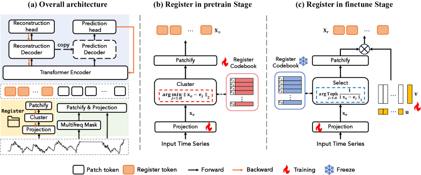
Figure 2: The model architecture of ROSE.

The time series forecasting paradigm of ROSE contains two steps: pre-training and fine-tuning. First, the model is pre-trained on large-scale datasets from various domains, with two pre-training tasks: reconstruction and prediction. We set up the self-supervised reconstruction task to help the model understand time series comprehensively and set the supervised prediction task to enhance the model’s few-shot learning ability. Then, ROSE fine-tunes with a target dataset in the downstream scenario.

As shown in Figure 2, ROSE employs the Encoder-Decoder architecture to model time series. The backbone consists of multiple Transformer layers to process sequential information and effectively capture temporal dependencies [33]. ROSE is pre-trained in a channel-independent way, which is widely used in time series forecasting [6].

Input Representations. To enhance the generalization of ROSE for adaptive transferring from multi-domains to different target domains, we model the inputs $\mathbf{x}$ with patch tokens and register tokens. Patch tokens are obtained by partitioning the time series using patching layers [6], to preserve local temporal information. Register tokens are obtained by linear mapping and clustering each of the entire time series input into discrete embedding, to capture domain-specific information, which will be introduced in Section 3.3.

3.2 Decomposed frequency learning

As shown in Figure 1, time series data are composed of multiple combined frequency components, resulting in overlapping of different temporal variations. Furthermore, low-frequency components typically contain information about overall trends and longer-scale variations, and high-frequency components usually contain information about short-term fluctuations and shorter-scale variations, therefore, understanding time series from low and high frequencies separately benefits general time series representation learning. Based on the observations above, we propose decomposed frequency learning based on multi-freq masking to understand the time series from multiple-frequency perspectives, which enhances the model’s ability to learn generalized representations.

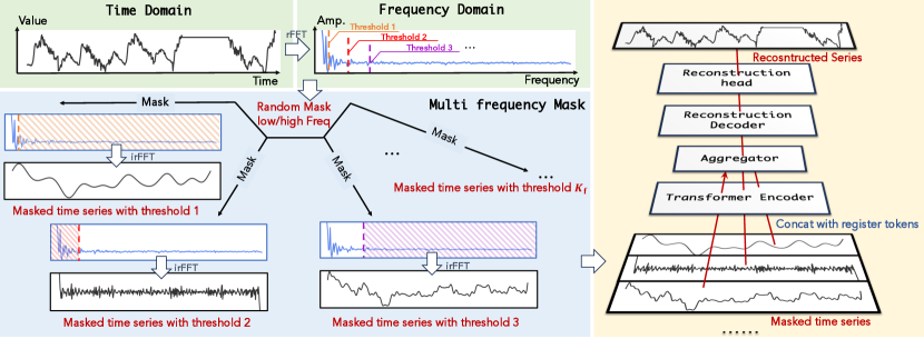
Figure 3: An illustration of decomposed frequency learning. Based on the pre-defined thresholds, we randomly apply low/high-frequency masking to the time series in the frequency domain and then transform it back to the time domain for reconstruction.

Multi-freq masking. Given a time series $\mathbf{x}\in\mathbb{R}^{L}$, we utilize the Real Fast Fourier Transform (rFFT) [34] to transform it into the frequency domain, giving rise to $\mathbf{x}_{\mathrm{freq}}\in\mathbb{R}^{L/2}$.

$$\mathbf{x}_{\mathrm{freq}}=\mathrm{rFFT}(\mathbf{x}).$$ (1)

To separately model high-frequency and low-frequency information in time series, we sample $K_{\mathrm{f}}$ thresholds ${\tau_{1},\tau_{2},\tau_{3},...,\tau_{K_{\mathrm{f}}}}$ and $K_{\mathrm{f}}$ random numbers ${\mu_{1},\mu_{2},\mu_{3},...,\mu_{K_{\mathrm{f}}}}$ for multi-frequency masks, where $\tau\in\mathrm{Uniform}(0,a)$, $a<L/2$ , and $\mu\in\mathrm{Bernoulli}(1,p)$. Each pair of $\tau_{i}$ and $\mu_{i}$ corresponds to the $i_{th}$ frequency mask. This generates a mask matrix $\mathbf{M}\in\{0,1\}^{K_{\mathrm{f}}\times L/2}$, where each row corresponds to the $i_{th}$ frequency mask, each column corresponds to the $j_{th}$ frequency, and each element $m_{ij}$ is 0 or 1, meaning that the $j_{th}$ frequency is masked with the $i_{th}$ frequency mask or not.

$$m_{ij}=\left\{\begin{aligned} &\quad\mu_{i}&,if\,\ \mathbf{x}_{\mathrm{freq}_{j}}<\tau_{i}\\ &(1-\mu_{i})&,if\,\ \mathbf{x}_{\mathrm{freq}_{j}}>\tau_{i}\end{aligned}\right.,$$ (2)

where $\tau_{i}$ and $\mu_{i}$ denote the threshold and random number for the $i_{th}$ frequency domain mask, $\mathbf{x}_{\mathrm{freq}_{j}}$ represents the $j_{th}$ frequency of $\mathbf{x}_{\mathrm{freq}}$. If $\mu_{i}=1$, it indicates masking of the high frequencies, whereas if $\mu_{i}=0$, it signifies the masking of the low frequencies.

After obtaining the mask matrix $\mathbf{M}$, we replicate $\mathbf{x}_{\mathrm{freq}}$ $K_{\mathrm{f}}$ times to get the $\mathbf{X}_{\mathrm{freq}}\in\mathbb{R}^{K_{\mathrm{f}}\times L/2}$ and perform element-wise Hadamard product with the mask matrix $\mathbf{M}$ to get masked frequency of time series. Then, we use the inverse Real Fast Fourier Transform (irFFT) to convert the results from the frequency domain back to the time domain and get $K_{\mathrm{f}}$ masked sequences $\mathbf{X}_{\mathrm{mask}}=\{\mathbf{x}_{\mathrm{mask}}^{i}\}_{i=1}^{K_{\mathrm{f}}}$, where each $\mathbf{x}_{\mathrm{mask}}^{i}\in\mathbb{R}^{L}$ corresponding to masking with a different threshold $\tau_{i}$.

$$\mathbf{X}_{\mathrm{mask}}=\mathrm{irFFT}(\mathbf{X}_{\mathrm{freq}}\odot\mathbf{M}).$$ (3)

Representation learning. After obtaining the $K_{\mathrm{f}}$ masked sequences $\mathbf{X}_{\mathrm{mask}}$, we divide each sequence $\mathbf{x}_{\mathrm{mask}}^{i}$ into $P$ non-overlapping patches, and use a linear layer to transforming them into $P$ patch tokens, and thus we get $\mathcal{X}_{\mathrm{mp}}=\{\mathbf{X}_{\mathrm{mp}}^{i}\}_{i=1}^{K_{\mathrm{f}}}$ to capture general information, where each $\mathbf{X}_{\mathrm{mp}}^{i}\in\mathbb{R}^{P\times D}$, and $D$ is the dimension for each patch token. We replicate the register tokens $\mathbf{X}_{\mathrm{u}}$ $K_{\mathrm{f}}$ times to get $\mathcal{X}_{\mathrm{u}}\in\mathbb{R}^{K_{\mathrm{f}}\times N_{\mathrm{r}}\times D}$, where $\mathbf{X}_{\mathrm{u}}\in\mathbb{R}^{N_{\mathrm{r}}\times D}$ is obtained by inputting the original sequence into the TS-Register, as detailed in Section 3.3. Then, we concatenate the patch tokens $\mathcal{X}_{\mathrm{mp}}$ with the register tokens $\mathcal{X}_{\mathrm{u}}$, and feed them into the transformer encoder to obtain the representation of each masked series. These representations are then aggregated to yield a unified representation $\mathbf{S}\in\mathbb{R}^{(N_{\mathrm{r}}+P)\times D}$:

$$\mathbf{S}=\mathrm{Aggregator(Encoder(Concatenate(\mathcal{X}_{mp},\mathcal{X}_{u})))}.$$ (4)

Reconstruction task. After obtaining the representation $\mathbf{S}$, we feed it into the reconstruction decoder and ultimately reconstruct the original sequence $\mathbf{\hat{x}}\in\mathbb{R}^{L}$ through the reconstruction head. As frequency domain masking affects the overall time series, we compute the Mean Squared Error (MSE) reconstruction loss for the entire time series.

$$\mathcal{L}_{\mathrm{reconstruction}}=\mathrm{||\mathbf{x}-\hat{\mathbf{x}}||_{2}^{2}}.$$ (5)

3.3 Time series register

By decomposed frequency learning, we can obtain the domain-general representations, and additionally, we propose the TS-Register that learns register tokens as the domain-specific information from the multi-domain datasets for adaptive transfer. It clusters domain-specific information from the multi-domain datasets into register tokens and stores such domain-specific information in the register codebook during pre-training. Then, it adaptively selects similar information from the register codebook to enhance the target domain during fine-tuning.

We set up a randomly initialized register codebook $\mathbf{E}\in\mathbb{R}^{H\times D_{\mathrm{r}}}$ with $H$ cluster center vectors $\mathbf{e}_{i}\in\mathbb{R}^{D_{\mathrm{r}}},i\in\{1,2,…,H\}$. Each of input time series $\mathbf{x}\in\mathbb{R}^{L}$ is projected into a data-dependent embedding $\mathbf{x}_{\mathrm{e}}\in\mathbb{R}^{D_{\mathrm{r}}}$ through a linear layer.

Pre-training stage. As shown in Figure 2(b), we use the register codebook to cluster these data-dependent embeddings, which generate domain-specific information, and store them in pre-training. Specifically, We find a cluster center vector $\mathbf{e}_{\delta}$ from the register codebook $\mathbf{E}$ where we use $\delta$ to denote the cluster that the data-dependent embedding $\mathbf{x}_{\mathrm{e}}$ belongs to, as shown in Equation 6.

$$\delta=\underset{j=1:H}{\arg\operatorname{min}}\left\|\mathbf{x}_{\mathrm{e}}-\mathbf{e}_{j}\right\|_{2}.$$ (6)

$$\mathcal{L}_{\text{register}}=\|\text{sg}(\mathbf{x}_{\mathrm{e}})-\mathbf{e}_{\delta}\|^{2}_{2}+\|\mathbf{x}_{\mathrm{e}}-\text{sg}(\mathbf{e}_{\delta})\|^{2}_{2}.$$ (7)

To update the cluster center vectors in the register codebook $\mathbf{E}$ that represent the domain information of the pre-trained datasets, we set the loss function shown in Equation 7 that minimizes the distance between the data-dependent embedding $\mathbf{x}_{\mathrm{e}}$ and the cluster center $\mathbf{e}_{\delta}$. $\text{sg}()$ refers to the stop gradient operation, and is used to solve the problem that the gradient of the $\arg\operatorname{min}$ function cannot be backpropagated [35]. The first term is used to update the register codebook $\mathbf{E}$, and the second term is used to update the parameters of the linear layer that learns $\mathbf{x}_{\mathrm{e}}$.

In this way, the vectors in the register codebook $\mathbf{E}$ cluster the embeddings of different data and learn the domain-specific centers for pre-trained datasets, which can represent domain-specific information. As a vector in the register codebook $\mathbf{E}$, $\mathbf{e}_{\delta}$ represents the domain-specific information for input $\mathbf{x}$. $\mathbf{e}_{\delta}$ is invariant under small perturbations in $\mathbf{x}_{\mathrm{e}}$ that represents $\mathbf{x}$, which promotes better representation of domain-specific information and robustness of the vectors in the register. This also avoids their over-reliance on detailed information about specific datasets [36].

The cluster center vector $\mathbf{e}_{\delta}$ is then patched into $\mathbf{X}_{\mathrm{u}}\in\mathbb{R}^{N_{\text{r}}\times D}$, where $N_{\text{r}}$ is the number of the register tokens and $D$ is the dimensionality of transformer latent space. $\mathbf{X}_{\mathrm{u}}$ is called register tokens, which are used as the prefix of the patch tokens $\mathbf{X}_{\mathrm{p}}\in\mathbb{R}^{P\times D}$ and input for the transformer encoder to provide domain-specific information.

Fine-tuning stage. As shown in Figure 2(c), after obtaining a register codebook $\mathbf{E}$ that contains domain-specific information through pre-training, we freeze the register parameters to adaptively use this domain-specific information in the downstream task.

Since the target domain may not strictly fit one of the upstream domains, learning the embedding of the downstream data employs a top-k strategy that selects top-k similar vectors in the register codebook. As shown in Equation 8, the embedding of input time series $\mathbf{x}_{\mathrm{e}}$ picks the $k$ nearest vectors in the register codebook $\mathbf{E}$, and uses their average as $\bar{\mathbf{e}}_{k}$ to represent the domain-specific information from the pre-train stage. $\bar{\mathbf{e}}_{k}$ is also patched into $\mathbf{X}_{\mathrm{d}}\in\mathbb{R}^{N_{\text{r}}\times D}$ and is used as the register tokens.

$$\bar{\mathbf{e}}_{k}=\frac{1}{k}\sum_{i=1}^{k}\mathbf{e}_{\delta_{i}},\ \ \left\{\delta_{1},\cdots,\delta_{k}\right\}=\underset{j=1:H}{\arg\operatorname{Topk}}(\frac{1}{\left\|\mathbf{x}_{\mathrm{e}}-\mathbf{e}_{j}\right\|_{2}}).$$ (8)

Since the downstream data has its own specific information at the dataset level in addition to the domain level, this may not be fully represented by the domain information obtained from the pre-trained dataset alone. Therefore, we additionally set a matrix $\mathbf{A}\in\mathbb{R}^{N_{\mathrm{r}}\times D}$ to adjust $\mathbf{X}_{\mathrm{d}}$ to complement the specific information of downstream data. Since the pre-trained model has a very low intrinsic dimension [37], in order to get better fine-tuning results, $\mathbf{A}$ is set as a low-rank matrix:

$$\mathbf{A}=\mathbf{u}\times\mathbf{v^{\mathrm{T}}},$$ (9)

where $\mathbf{u}\in\mathbb{R}^{N_{\mathrm{r}}}$ and $\mathbf{v}\in\mathbb{R}^{D}$, and only the vectors $\mathbf{u}$ and $\mathbf{v}$ need to be retrained in the fine-tuning step. As illustrated in Equation 10, the register token $\mathbf{X}_{\mathrm{r}}$ of the downstream scenario is obtained by doing the Hadamard product of $\mathbf{X}_{\mathrm{d}}$, which represents the domain-specific information obtained at the pre-train stage, and $\mathbf{A}$, which represents the downstream dataset-specific information.

$$\mathbf{X}_{\mathrm{r}}=\mathbf{X}_{\mathrm{d}}\odot\mathbf{A}.$$ (10)

3.4 Training

To improve the model’s prediction ability when only few samples are available downstream, we co-train supervised prediction with self-supervised reconstruction that uses multi-frequency mask to learn unified features that are more applicable to the downstream prediction task.

Prediction task. The input time series $\mathbf{x}\in\mathbb{R}^{L}$ is sliced into $P$ non-overlapping patches and then mapped to $\mathbf{X}_{\mathrm{p}}\in\mathbb{R}^{P\times D}$. Based on common forecasted needs [1], we set up four prediction heads mapping to prediction lengths of $\{96,192,336,720\}$ to accomplish the prediction task. Patch tokens $\mathbf{X}_{\mathrm{p}}$ are concatenated with the register tokens $\mathbf{X}_{\mathrm{u}}$ and then successively fed into the transformer encoder, prediction decoder, and prediction heads to obtain four prediction results$\mathbf{\hat{Y}}_{F}$, where $F\in\{96,192,336,720\}$. With the ground truth $\mathbf{Y}_{F}$, the prediction loss $\mathcal{L}_{\text{prediction}}$ is shown in Equation 11.

$$\mathcal{L}_{\text{prediction}}=\sum_{F\in\{96,192,336,720\}}||{\mathbf{Y}_{F}-{\mathbf{\hat{Y}}_{F}}}||_{2}^{2}.$$ (11)

Pre-training. The reconstruction task learns generalized features through the transformer encoder and reconstruction decoder. To utilize these features for the prediction task, the parameters of the reconstruction decoder are copied to the prediction decoder during forward propagation. To avoid prediction training affecting the generalization performance of the model, the gradients of the prediction heads are skipped at back-propagation. The overall pre-training loss is shown in Equation 12.

$$\mathcal{L_{\text{pre-train}}}=\mathcal{L}_{\text{reconstruction}}+\mathcal{L}_{\text{prediction}}+\mathcal{L}_{\text{register}}.$$ (12)

Fine-tuning. We only perform a prediction task in fine-tuning. Patch tokens $\mathbf{X}_{\text{p}}$ are concatenated with the adjusted register tokens $\mathbf{X}_{\mathrm{r}}$. For a downstream task with a fixed prediction length, we use the corresponding pre-trained prediction head to fine-tune the model.

4 Experiments

Pre-training datasets. Large-scale datasets are crucial for pre-training a general time series forecasting model. In light of this, we gather a considerable amount of publicly available datasets from various domains, including energy, nature, health, transport, web, and economics, etc. The details of these datasets are shown in the Appendix A.1. To enhance data utilization, we downsampled fine-grained datasets to coarser granularity, resulting in approximately 886 million time points.

Evaluation datasets. To conduct comprehensive and fair comparisons for different models, we conducted experiments on eight real-world benchmarks as the target datasets, including Weather, Solar, Traffic, Electricity, and ETT (4 subsets), which cover multiple domains.

Baselines. We select the state-of-the-art models as our baselines, including Transformer-based models: Timer [2], iTransformer [20], and PatchTST [6]; CNN-based model: TimesNet [18]; MLP-based models: FITS [38], TIDE [39], and DLinear [40]. It is worth noting that Timer is a recent general time series model with a GPT-style architecture. Since the size of the look-back window can affect the performance of different models, we choose the look-back window size in $\{96,336,512,720\}$ for each baseline that achieves its best results for fair comparisons.

Setup. Consistent with previous works, we adopted Mean Squared Error (MSE) and Mean Absolute Error (MAE) as evaluation metrics. All methods predict the future values with lengths $F=\{96,192,336,720\}$. More implementation details are presented in the Appendix A.3.

4.1 Main results

Full-shot setting. We first pre-train ROSE on our pre-training datasets and then fine-tune with full downstream data (full-shot setting). Similarly, all baselines are also run in the same full-shot setting. As shown in Table 1, we also present the results of the ROSE in 10% few-shot setting, where the model uses the same validation and test data but is only fine-tuned with 10% training data of each target dataset. Key observations are summarized as follows. First, as a general forecasting model, ROSE achieves superior performance compared to the seven state-of-the-art baselines with full-data training, especially Timer, which shows that our decomposed frequency learning and register help to learn generalized representations from large-scale datasets and adaptively transfer the multi-domain information to specific downstream scenarios. Second, we observe that ROSE achieves competitive performance in 10% few-shot setting, even compared to baselines trained with full data. This observation validates the transferability of ROSE pre-trained with large multi-source data.

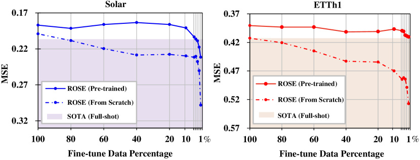
Figure 4: The forecasting results of ROSE obtained by training from scratch and fine-tuning from the pre-trained model. The right, upper corner is the best case.

Few-shot setting. We also compared all models under the 10% few-shot setting in Table 9 in Appendix H.2. We can see that ROSE performs the best on all eight datasets in the scenarios where the training data are rare in the target domain, surpassing extensive advanced models. Figure 4 shows the results of pre-trained ROSE and ROSE trained from scratch on the Solar and ETTh1 with different fine-tuning data percentages, noting the best baselines in full-shot setting. The pre-trained ROSE shows stable, superior performance even with limited fine-tuned samples. Specifically, the pre-trained ROSE achieves performance that surpasses the SOTA with only 5% for Solar and 1% data for ETTh1. Moreover, compared to the ROSE trained from scratch, the pre-trained ROSE exhibits a slower decline in predictive performance with the reduction of fine-tuning data, demonstrating the impressive generalization ability of ROSE through large-scale pre-training.

Table 1: The results for ROSE in full-shot setting and 10% few-shot setting, compared with other methods in full-shot setting. The average results of all predicted lengths are listed here.

Models	ROSE		ROSE 10%		Timer		ITransformer		PatchTST		FITS		TimesNet		TiDE		DLinear
Metric	MSE	MAE	MSE	MAE	MSE	MAE	MSE	MAE	MSE	MAE	MSE	MAE	MSE	MAE	MSE	MAE	MSE	MAE
ETTm1	0.341	0.367	0.349	0.372	0.436	0.456	0.407	0.410	0.353	0.382	0.355	0.379	0.400	0.406	0.355	0.378	0.357	0.379
ETTm2	0.246	0.305	0.249	0.308	0.308	0.351	0.288	0.332	0.256	0.317	0.249	0.312	0.291	0.333	0.249	0.312	0.267	0.332
ETTh1	0.391	0.414	0.397	0.419	0.483	0.459	0.454	0.447	0.413	0.434	0.407	0.429	0.458	0.450	0.419	0.430	0.423	0.437
ETTh2	0.330	0.374	0.335	0.380	0.366	0.406	0.383	0.407	0.331	0.381	0.333	0.382	0.414	0.427	0.345	0.394	0.431	0.447
Traffic	0.390	0.264	0.418	0.278	0.413	0.284	0.428	0.282	0.391	0.264	0.410	0.282	0.62	0.336	0.356	0.261	0.434	0.295
Weather	0.217	0.251	0.224	0.252	0.277	0.306	0.246	0.298	0.226	0.264	0.218	0.260	0.259	0.287	0.236	0.282	0.246	0.300
Solar	0.188	0.215	0.192	0.216	0.251	0.262	0.233	0.262	0.207	0.294	0.223	0.264	0.301	0.319	0.223	0.288	0.230	0.295
Electricity	0.155	0.248	0.164	0.253	0.181	0.274	0.178	0.270	0.159	0.253	0.163	0.257	0.192	0.295	0.159	0.257	0.166	0.264

4.2 Ablation studies

Model architecture. To validate effectiveness of our model design, we perform ablation studies on TS-Register, prediction tasks, and reconstruction task in 10% few-shot setting. Table 2 shows the impact of each module. The TS-Register leverages multi-domain information during pre-training, aiding adaptive transfer to downstream datasets, as further discussed in section 4.4. The prediction tasks enhance performance in data-scarce situations. Without it, performance significantly drops on ETTh1 and ETTh2 with limited samples. Without the reconstruction task, our model shows negative transfer effects on ETTm1 and ETTm2, likely due to the prediction task making the model more susceptible to pre-training data biases.

Mask method.

To further validate the effectiveness of decomposed frequency learning, we replace the multi-frequency masking with different masking methods, including two mainstream time-domain methods: patch masking [6] and multi-patch masking [5], as well as a single frequency masking, which masks time series in the frequency domain only once. The results show that frequency domain modeling yields superior performance improvements compared to time-domain modeling. Additionally, we observe that applying multi-frequency masking results in enhanced outcomes, thus affirming that incorporating a multi-frequency perspective significantly aids the model in more accurately comprehending temporal patterns.

Table 2: Ablations on ROSE. We replace different masking methods, in addition to component removal. The average results of all predicted lengths are listed here.

Design		ETTm1		ETTm2		ETTh1		ETTh2
		MSE	MAE	MSE	MAE	MSE	MAE	MSE	MAE
ROSE		0.349	0.372	0.250	0.308	0.397	0.419	0.335	0.380
Replace Multi-Freq Masking	Single Freq Masking	0.354	0.379	0.257	0.313	0.403	0.423	0.347	0.387
	Multi Patch Masking	0.356	0.379	0.259	0.316	0.404	0.426	0.349	0.389
	Patch Masking	0.378	0.4	0.261	0.319	0.408	0.432	0.375	0.407
w/o	TS-Register	0.354	0.378	0.256	0.312	0.418	0.427	0.355	0.39
	Predict Task	0.36	0.384	0.257	0.314	0.422	0.438	0.372	0.41
	Reconstruct Task	0.387	0.403	0.269	0.327	0.412	0.428	0.361	0.399
From Scratch		0.370	0.393	0.261	0.318	0.470	0.480	0.401	0.425

4.3 Scalability

Scalability is crucial for a general model, enabling significant performance improvements by expanding pre-training data and model sizes. To investigate the scalability of ROSE, we increased both the model size and dataset size and evaluated its predictive performance on four ETT datasets.

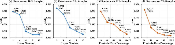
Figure 5: (a)/(b): Larger ROSE demonstrates better performance on downstream forecasting. (c)/(d): ROSE pre-trained on larger datasets demonstrates better performance on downstream forecasting.

Model size. Constrained by computational resources, we use 40% pre-training datasets. The results are shown in Figure 5(a) and (b). When maintaining the model dimension, we increased the model layers, increasing model parameters from 2M to 4.5M. This led to 10.37% and 9.34% improvements in the few-shot scenario with 5% and 10% downstream data, respectively.

Data size. When keeping the model size, we increase the size of the pre-training datasets from 178M to 886M. The results are shown in Figure 5(c) and (d). The performance of our model steadily improves with the increase in dataset size and achieves improvements of 7.4% and 4.8% respectively.

4.4 Model Analysis

Zero-shot and inference efficiency. By adopting the dual pre-train task, our model possesses strong generalization ability and can forecast without requiring any downstream data for fine-tuning.

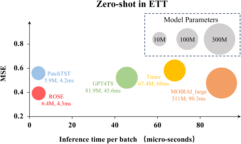
Figure 6: Model performance in zero-shot setting comparison and inference efficiency comparison.

To validate ROSE’s zero-shot capabilities and assess its inference efficiency, we compared it with other models that have recently demonstrated similar abilities, namely Timer [2], MOIRAI [8], PatchTST [6], and GPT4TS [10]. Specific implementation details and results can be found in Appendix B. As shown in Figure 6, ROSE exhibits superior performance in zero-shot setting, with significantly fewer model parameters and inference time compared to other models. This underscores the robust generalization and scalability of ROSE.

Visualization of TS-Register. To validate the TS-Register’s capability to transfer domain-specific information adaptively from pre-training datasets to target datasets, we visualize the cosine similarity of register vector selections from datasets across different domains. As shown in Figure 7(a), the cosine similarity is higher for datasets within the same domain and lower between different domains. We also visualize the register vector selections from different datasets in Figures 7(b) and (c), where datasets from the same domain show similar visualizations. This confirms the TS-Register’s capability of adaptive transfer from multi-source to target datasets across various domains.

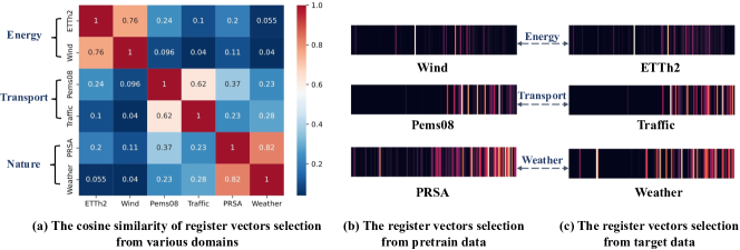
Figure 7: Visualization of TS-Register.

Sensitivity. The sensitivity analyses for the upper bound $a$ of the thresholds, the number of masked series $K_{\mathrm{f}}$, the number of register tokens $N_{\text{r}}$ and the size of codebook $H$ are presented in Appendix C.

5 Conclusion and future work

In this work, we propose ROSE, a novel general model, addressing the challenges of leveraging multi-domain datasets for enhancing downstream prediction task performance. ROSE utilizes decomposed frequency learning and TS-Register to capture generalized and domain-specific representations, enabling improved fine-tuning results, especially in data-scarce scenarios. Our experiments demonstrate ROSE’s superior performance over baselines with both full-data and few-data fine-tuning, as well as its impressive zero-shot capabilities. Future efforts will concentrate on expanding pre-training datasets and extending ROSE’s applicability across diverse time series analysis tasks, e.g., classification.

Appendix A IMPLEMENTATION DETAILS

A.1 Pre-training Datasets

We use multi-source datasets in pre-training which contain subsets of Monash [41], UEA [42] and UCR [43] time series regression datasets, as well as some other time series classical datasets [44, 45, 46, 47, 48]. The final list of all pre-training datasets is shown in Table 4. There is no overlap between the pre-training datasets and the target datasets. It is worth noting that the dataset weather in the pre-training dataset is a univariate dataset, which is different to the multivariate dataset weather in the target task. The pre-trained datasets can be categorized into 6 different domains according to their sources: Energy, Nature, Health, Transport, and Web. The sampling frequencies of the datasets show a remarkable diversity, ranging from millisecond samples to monthly samples, which reflects the diverse application scenarios and complexity of the real world. For all pre-training datasets, we split them into univariate sequences and train them in a channel-independent manner.

A.2 Evaluation Datasets

We use the following 8 multivariate time-series datasets for downstream fine-tuning and forecasting: ETT datasets contain 7 variates collected from two different electric transformers from July 2016 to July 2018. ETT datasets consist of four subsets, of which ETTh1/ETTh2 are recorded hourly and ETTm1/ETTm2 are recorded every 15 minutes. Traffic contains road occupancy rates measured by 862 sensors on freeways in the San Francisco Bay Area from 2015 to 2016, recorded hourly. Weather collects 21 meteorological indicators, such as temperature and barometric pressure, for Germany in 2020, recorded every 10 minutes. Solar records solar power generation from 137 PV plants in 2006, every 10 minutes. Electricity contains the electricity consumption of 321 customers from July 2016 to July 2019, recorded hourly. We split each evaluation dataset into train-validation-test sets and detailed statistics of evaluation datasets are shown in Table 3.

Table 3: The statistics of evaluation datasets

Dataset	ETTm1	ETTm2	ETTh1	ETTh2	Traffic	Weather	Solar	Electricity
Variables	7	7	7	7	862	21	137	321
Timestamps	69680	69680	17420	17420	17544	52696	52560	26304
Split Ratio	6:2:2	6:2:2	6:2:2	6:2:2	7:1:2	7:1:2	7:1:2	7:1:2

Table 4: List of pretraining datasets.

Domain	Dataset	Frequency	Time Pionts	Source
Energy	Aus. Electricity Demand	Half Hourly	1155264	Monash[41]
	Wind	4 Seconds	7397147	Monash[41]
	Wind Farms	Minutely	172178060	Monash[41]
	London Smart Meters	Half Hourly	166527216	Monash[41]
Nature	Phoneme	-	2160640	UCR[43]
	EigenWorms	-	27947136	UEA[42]
	PRSA	Hourly	4628448	[44]
	Temperature Rain	Daily	23252200	Monash[41]
	StarLightCurves	-	9457664	UCR[43]
	Worms	0.033 Seconds	232200	UCR[43]
	Saugeen River Flow	Daily	23741	Monash[41]
	Sunspot	Daily	73924	Monash[41]
	Weather	Daily	43032000	Monash[41]
	KDD Cup 2018	Daily	2942364	Monash[41]
	US Births	Daily	7305	Monash[41]
Health	MotorImagery	0.001 Seconds	72576000	UEA[42]
	SelfRegulationSCP1	0.004 Seconds	3015936	UEA[42]
	SelfRegulationSCP2	0.004 Seconds	3064320	UEA[42]
	AtrialFibrillation	0.008 Seconds	38400	UEA[42]
	PigArtPressure	-	624000	UCR[43]
	PIGCVP	-	624000	UCR[43]
	TDbrain	0.002 Seconds	79232703	[45]
Transport	Pems03	5 Minute	9382464	[46]
	Pems04	5 Minute	5216544	[46]
	Pems07	5 Minute	24921792	[46]
	Pems08	5 Minute	3035520	[46]
	Pems-bay	5 Minute	16937700	[46]
	Pedestrian_Counts	Hourly	3132346	Monash[41]
Web	Web Traffic	Daily	116485589	Monash[41]
Economic	FRED_MD	Monthly	77896	[47]
	Bitcoin	Daily	75364	Monash[41]
	NN5	Daily	87801	[48]

A.3 Setting

We implemented ROSE in PyTorch [49] and all the experiments were conducted on 8 NVIDIA A800 80GB GPU. We used ADAM [50] with an initial learning rate of $5\times 10^{-4}$ and implemented learning rate decay using the StepLR method to implement learning rate decaying pre-training. By default, ROSE contains 3 encoder layers and 3 decoder layers with head number $H=16$ and the dimension of latent space $D=256$.

Pre-training. We use $N_{\mathrm{r}}=3$ as the number of register tokens and $P=8$ as the path tokens. We set the input length to 512 for the supervised prediction task with target lengths of 96, 192, 336, and 720. We also set the input length to 512 for self-supervised multi-frequency mask-reconstruction task, where mask number $K_{\mathbf{f}}=4$. The batch size is set to 8192 in pre-training.

Fine-tuning. We fix the lookback window to 512, and perform predictions with target lengths of 96, 192, 336, and 720, respectively. The number of register tokens $N_{\mathrm{r}}$ and patch tokens $P$ is the same as in pre-training, and the parameter $k=3$ in topk is set when selection vectors are performed in the register codebook. The batch size is set to 64 in fine-tuning.

A.4 Baselines

We select the state-of-the-art methods as our baselines to compare the performance of different models with full-data fine-tuning and 10% few-shot setting, including Transformer-based methods: Timer [2], iTransformer [20], and PatchTST [6]; CNN-based backbones method: TimesNet [18]; MLP-based methods: FITS [38], TIDE [39], and DLinear [40]. It is worth noting that Timer is a recent general time series model with a GPT-style architecture. Since the size of the look-back window can affect the performance of different models, we choose the look-back window size in $\{96,336,512,720\}$ for each baseline that achieves its best results for fair comparisons. The specific code base for these models is listed in Table 5:

Table 5: Code repositories for baselines

Baselines	code repositories
Timer	https://github.com/thuml/Large-Time-Series-Model
iTransformer	https://github.com/thuml/iTransformer
PatchTST	https://github.com/yuqinie98/PatchTST
FITS	https://anonymous.4open.science/r/FITS/README.md
TimesNet	https://github.com/thuml/TimesNet
TIDE	https://github.com/google-research/google-research/tree/master/tide
Dlinear	https://github.com/cure-lab/LTSF-Linear

Appendix B Zero shot and inference efficiency

To explore the inference efficiency and zero-shot capability of ROSE, we selected recent models with zero-shot capability, including Timer [2] and MOIRAI [8], as well as models with the potential for zero-shot learning, including PatchTST [6] and GPT4TS [10], for comparison on the ETT dataset. And we evaluate their inference efficiency by recording inference time per batch on the ETTh2 dataset with a batch size of 32.

Pre-train: We select the models with the largest parameter weights for Timer and MOIRAI as baselines. GPT4TS and PatchTST were pre-trained on our pre-training dataset with prediction tasks to acquire zero-shot capability. The specific settings are shown in the table 6.

Detailed results: For fare comparison, we set the input length as 96, 336, 512, and 720 for all zero-shot baseline models. We do not consider longer input length, as many real-world scenarios could offer very limited samples, and thus the zero-shot setting with only a few samples is crucial for them. As the baselines do not contain results with this setting in their original papers, we rerun them and report their best results in Table 11. ROSE consistently surpasses the baselines despite having significantly fewer parameters and inference time.

Table 6: Pre-train setting and inference efficiency

Model	Parameters	Pre-train data size	Inference time per batch	code repositories
ROSE	6.4M	0.89B	4.3 ms	-
MOIRAI_large	311M	27B	90.3ms	https://github.com/redoules/moirai
GPT4TS	81.9M	0.89B	45.6 ms	https://github.com/DAMO-DI-ML/NeurIPS2023-One-Fits-All
Timer	67.4M	1B	68 ms	https://github.com/thuml/Large-Time-Series-Model
PatchTST	5.9M	0.89B	4.2 ms	https://github.com/PatchTST/PatchTST

Appendix C Sensitivity

Number of masked series. As described in Section 3.2, we propose decomposed frequency learning, which employs multiple thresholds to randomly mask high and low frequencies in the frequency domain, thereby decomposing the original time series into multiple frequency components. This allows the model to understand the time series from multiple frequency perspectives. In this experiment, we study the influence of the number of masked series $K_{m}athrm{f}$ on downstream performance. We train ROSE with 1, 2, 3, 4, 5, or 6 mask series. We report the results of this analysis in Figure 8(a). We find that as the number of masked sequences increases, the downstream performance gradually improves. This is because the model can better understand the time series from the decomposed frequency components, which enhances the model’s generalization ability. However, more masked series do not bring better downstream performance. This could be due to an excessive number of masked sequences leading to information redundancy. In all our experiments, we kept 4 mask series.

Number of register tokens. The TS-register module presented in Section 3.3 supports the configuration of an arbitrary number of register tokens. In Figure 8(b), we visualize the relationship between the performance on the ETT datasets under a 10% few-shot setting and the number of register tokens. It is observed that when the number of register tokens ranges from 1 to 6, the model’s performance remains relatively stable, with an optimal outcome achieved when the number is set to 3. This phenomenon may be because when the number of register tokens is too small, they contain insufficient domain-specific information, which limits their effectiveness in enhancing the model’s performance. Conversely, an excess of register tokens may introduce redundant information, hindering the accurate representation of domain-specific information. Additionally, we compared the results without the adjustment of a low-rank matrix on the register tokens and found that the incorporation of a low-rank matrix adjustment led to improvements across all quantities of register tokens. This finding underscores the significance of utilizing a low-rank matrix to supplement the register tokens with downstream data-specific information.

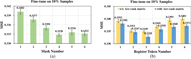
Figure 8: (a): Analysis of the number of masked series. (b): Analysis of the number of register tokens

Thresholds upper bound. Figure 9(a) illustrates the relationship between threshold upper bound and model performance. We have observed that the upper bound of the threshold has a minimal impact on the model’s performance. Generally, the information density is higher in low-frequency components compared to high-frequency ones. Therefore, the upper bound of the threshold should be biased towards the low-frequency range to balance the information content between low-frequency and high-frequency components. However, this bias should not be excessive. Our experiments indicate that an upper bound of $L/10$ performs worse than $L/5$ as an overly left-skewed threshold results in insufficient information in the low-frequency range, making the reconstruction task either too difficult or too simple. Based on our findings, we recommend using $L/5$ as the upper bound for the threshold.

Register codebook size. Figure 9(b) illustrates the relationship between register codebook size and model performance. The codebook size determines the upper limit of domain-specific information that the register can store. We can observe that there is a significant improvement in the model effect when the codebook size is increased from 32 to 128. When the codebook size exceeds 128, the improvement of the model effect with the increase of codebook size is no longer obvious. Therefore, we believe that 128 is an appropriate codebook size for the current pre-training datasets.

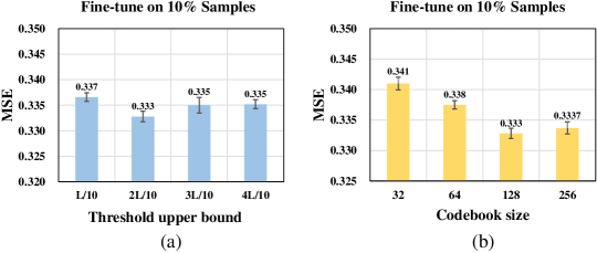
Figure 9: (a): Analysis of the threshold upper bound. (b): Analysis of the size of codebook

Appendix D Model generality

We evaluate the effectiveness of our proposed Multiple Frequency Mask (MFM) on Transformer-based models and CNN-based models, whose results are shown in Table 7. It is notable that MFM consistently improves these forecasting models. Specifically, it achieves average improvements of 6.3%, 3.7%, 1.5% in Autoformer [19], TimesNet [18], and PatchTST [6], respectively. This indicates that MFM can be widely utilized across various time series forecasting models to learn generalized time series representations and improve prediction accuracy.

Table 7: Performance Multiple Frequency Masking.

Datasets	ETTm1		ETTm2		ETTh1		ETTh2
Metric	MSE	MAE	MSE	MAE	MSE	MAE	MSE	MAE
Autoformer +Multi Freq Mask	0.600	0.521	0.328	0.365	0.493	0.487	0.452	0.458
	0.549	0.488	0.306	0.349	0.474	0.478	0.406	0.425
TimesNet +Multi Freq Mask	0.4	0.406	0.291	0.333	0.458	0.45	0.414	0.427
	0.386	0.398	0.282	0.324	0.446	0.438	0.386	0.403
PatchTST +Multi Freq Mask	0.353	0.382	0.256	0.317	0.413	0.434	0.331	0.381
	0.347	0.372	0.252	0.308	0.405	0.424	0.337	0.379

Appendix E Visualization of forecasting results

To provide a distinct comparison among different models, we present visualizations of the forecasting results on the ETTh2 dataset and the weather dataset in different settings, as shown in Figures 10 to Figures 13, given by the following models: DLinear [40], TimesNet [18], iTransfomrer [20], PatchTST [6], and TiDE [39]. Among the methods, ROSE demonstrates the most accurate prediction ability.

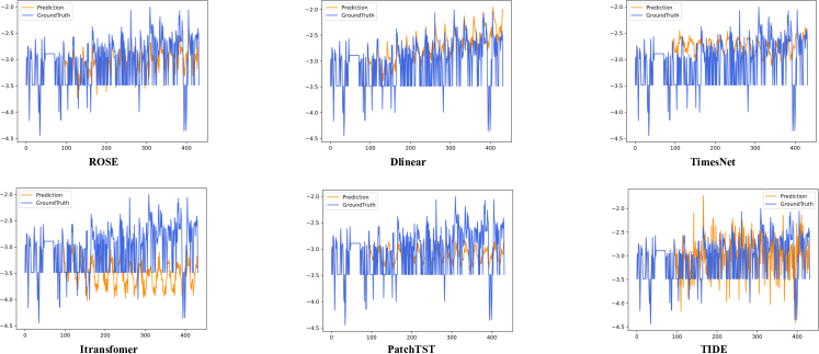
Figure 10: Visualization of input-512 and predict-336 forecasting results on the ETTh2 dataset with full-sample.

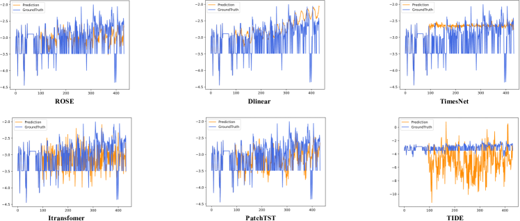
Figure 11: Visualization of input-512 and predict-336 forecasting results on the ETTh2 dataset with 10% samples.

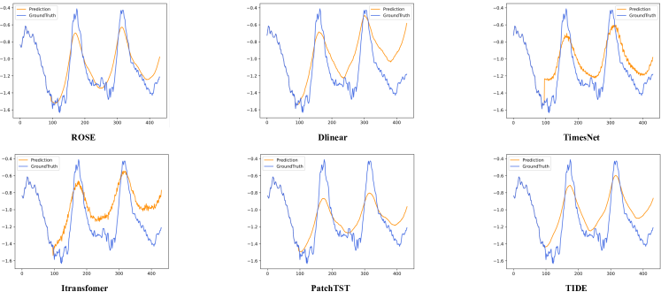
Figure 12: Visualization of input-512 and predict-336 forecasting results on the weather dataset with full-sample.

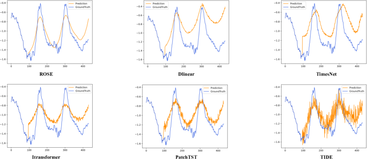
Figure 13: Visualization of input-512 and predict-336 forecasting results on the weather dataset with 10%-sample.

Appendix F Limitations

Our pre-training datasets still have room for expansion. While ROSE demonstrates strong performance, its effectiveness could be enhanced with a larger and more diverse set of pre-training datasets. By collecting additional real-world scenario data for pre-training, we aim to further improve the robustness and generalizability of ROSE across various domains.

Appendix G Broader Impacts

This paper presents ROSE, a novel general time series forecasting model that demonstrates promising performance. ROSE performs well in few-shot scenarios and shows notable zero-shot capabilities, highlighting its scalability and efficiency. We believe it can be a valuable addition to the pre-training research community. To support future research, we will also release the codebase for time-series pre-training.

This paper only focuses on the algorithm design. Using all the codes and datasets strictly follows the corresponding licenses A.1. There is no potential ethical risk or negative social impact.

Appendix H Full Results

H.1 Full-shot results

Table 8: Full results in full-shot setting.

Models		ROSE		Timer		ITransformer		PatchTST		FITS		Timesnet		TiDE		Dlinear
Metric		MSE	MAE	MSE	MAE	MSE	MAE	MSE	MAE	MSE	MAE	MSE	MAE	MSE	MAE	MSE	MAE
ETTm1	96	0.275	0.328	0.339	0.383	0.334	0.368	0.293	0.346	0.303	0.352	0.338	0.375	0.306	0.349	0.299	0.343
	192	0.324	0.358	0.396	0.430	0.377	0.391	0.333	0.370	0.337	0.368	0.374	0.387	0.335	0.366	0.335	0.365
	336	0.354	0.377	0.451	0.471	0.426	0.420	0.369	0.392	0.366	0.385	0.410	0.411	0.364	0.384	0.369	0.386
	720	0.411	0.407	0.558	0.540	0.491	0.459	0.416	0.420	0.415	0.411	0.478	0.450	0.413	0.413	0.425	0.421
	avg	0.341	0.367	0.436	0.456	0.407	0.410	0.353	0.382	0.355	0.379	0.400	0.406	0.355	0.378	0.357	0.379
ETTm2	96	0.157	0.243	0.184	0.263	0.180	0.264	0.166	0.256	0.162	0.253	0.187	0.267	0.161	0.251	0.167	0.260
	192	0.213	0.283	0.278	0.334	0.250	0.309	0.223	0.296	0.216	0.291	0.249	0.309	0.215	0.289	0.224	0.303
	336	0.266	0.319	0.334	0.375	0.311	0.348	0.274	0.329	0.268	0.326	0.321	0.351	0.267	0.326	0.281	0.342
	720	0.347	0.373	0.435	0.431	0.412	0.407	0.362	0.385	0.348	0.378	0.408	0.403	0.352	0.383	0.397	0.421
	avg	0.246	0.305	0.308	0.351	0.288	0.332	0.256	0.317	0.249	0.312	0.291	0.333	0.249	0.312	0.267	0.332
ETTh1	96	0.354	0.385	0.358	0.345	0.386	0.405	0.370	0.400	0.372	0.402	0.384	0.402	0.375	0.398	0.375	0.399
	192	0.389	0.407	0.438	0.448	0.441	0.436	0.413	0.429	0.404	0.422	0.436	0.429	0.412	0.422	0.405	0.416
	336	0.406	0.422	0.491	0.484	0.487	0.458	0.422	0.440	0.427	0.438	0.491	0.469	0.435	0.433	0.439	0.443
	720	0.413	0.443	0.644	0.559	0.503	0.491	0.447	0.468	0.424	0.454	0.521	0.500	0.454	0.465	0.472	0.490
	avg	0.391	0.414	0.483	0.459	0.454	0.447	0.413	0.434	0.407	0.429	0.458	0.450	0.419	0.430	0.423	0.437
ETTh2	96	0.265	0.320	0.288	0.346	0.297	0.349	0.274	0.337	0.271	0.336	0.340	0.374	0.270	0.336	0.289	0.353
	192	0.328	0.369	0.380	0.409	0.380	0.400	0.341	0.382	0.331	0.374	0.402	0.414	0.332	0.380	0.383	0.418
	336	0.353	0.391	0.372	0.413	0.428	0.432	0.329	0.384	0.354	0.395	0.452	0.452	0.360	0.407	0.448	0.465
	720	0.376	0.417	0.425	0.456	0.427	0.445	0.379	0.422	0.377	0.423	0.462	0.468	0.419	0.451	0.605	0.551
	avg	0.330	0.374	0.366	0.406	0.383	0.407	0.331	0.381	0.333	0.382	0.414	0.427	0.345	0.394	0.431	0.447
Traffic	96	0.354	0.252	0.351	0.255	0.395	0.268	0.360	0.249	0.385	0.271	0.593	0.321	0.336	0.253	0.410	0.282
	192	0.377	0.257	0.387	0.269	0.417	0.276	0.379	0.256	0.397	0.275	0.617	0.336	0.346	0.257	0.423	0.287
	336	0.396	0.262	0.426	0.288	0.433	0.283	0.392	0.264	0.410	0.280	0.629	0.336	0.355	0.260	0.436	0.296
	720	0.434	0.283	0.489	0.323	0.467	0.302	0.432	0.286	0.448	0.301	0.640	0.350	0.386	0.273	0.466	0.315
	avg	0.390	0.264	0.413	0.284	0.428	0.282	0.391	0.264	0.410	0.282	0.620	0.336	0.356	0.261	0.434	0.295
Weather	96	0.145	0.182	0.154	0.208	0.174	0.214	0.149	0.198	0.143	0.195	0.172	0.220	0.166	0.222	0.176	0.237
	192	0.183	0.226	0.243	0.287	0.221	0.254	0.194	0.241	0.186	0.238	0.219	0.261	0.209	0.263	0.220	0.282
	336	0.232	0.267	0.329	0.345	0.278	0.296	0.245	0.282	0.236	0.277	0.280	0.306	0.254	0.301	0.265	0.319
	720	0.309	0.327	0.384	0.384	0.358	0.347	0.314	0.334	0.307	0.330	0.365	0.359	0.313	0.340	0.323	0.362
	avg	0.217	0.251	0.277	0.306	0.258	0.278	0.226	0.264	0.218	0.260	0.259	0.287	0.236	0.282	0.246	0.300
Solar	96	0.171	0.199	0.230	0.245	0.203	0.237	0.190	0.273	0.198	0.253	0.250	0.292	0.200	0.270	0.206	0.281
	192	0.185	0.215	0.249	0.261	0.233	0.261	0.204	0.302	0.218	0.262	0.296	0.318	0.219	0.285	0.225	0.291
	336	0.193	0.218	0.255	0.265	0.248	0.273	0.212	0.293	0.235	0.270	0.319	0.330	0.234	0.296	0.240	0.300
	720	0.198	0.224	0.272	0.276	0.249	0.275	0.221	0.310	0.241	0.273	0.338	0.337	0.242	0.303	0.248	0.307
	avg	0.187	0.214	0.251	0.262	0.233	0.262	0.207	0.294	0.223	0.264	0.301	0.319	0.223	0.288	0.230	0.295
Electricity	96	0.125	0.220	0.136	0.230	0.148	0.240	0.129	0.222	0.134	0.231	0.168	0.272	0.132	0.229	0.140	0.237
	192	0.142	0.235	0.168	0.260	0.162	0.253	0.147	0.240	0.149	0.244	0.184	0.289	0.147	0.243	0.153	0.249
	336	0.162	0.252	0.192	0.285	0.178	0.269	0.163	0.259	0.165	0.260	0.198	0.300	0.161	0.261	0.169	0.267
	720	0.191	0.284	0.230	0.322	0.225	0.317	0.197	0.290	0.203	0.293	0.220	0.320	0.196	0.294	0.203	0.301
	avg	0.155	0.248	0.181	0.274	0.178	0.270	0.159	0.253	0.163	0.257	0.193	0.295	0.159	0.257	0.166	0.264

H.2 Few-shot results

Table 9: Full results in 10% few-shot setting

Models		ROSE		Timer		ITransformer		PatchTST		FITS		Timesnet		TiDE		Dlinear
Metric		MSE	MAE	MSE	MAE	MSE	MAE	MSE	MAE	MSE	MAE	MSE	MAE	MSE	MAE	MSE	MAE
ETTm1	96	0.287	0.336	0.351	0.398	0.353	0.392	0.317	0.363	0.311	0.354	0.481	0.446	0.373	0.388	0.454	0.475
	192	0.331	0.362	0.429	0.448	0.385	0.410	0.351	0.382	0.351	0.378	0.621	0.491	0.406	0.403	0.575	0.548
	336	0.362	0.379	0.496	0.495	0.422	0.432	0.376	0.398	0.377	0.396	0.521	0.479	0.436	0.425	0.773	0.631
	720	0.416	0.412	0.573	0.573	0.494	0.472	0.435	0.430	0.441	0.436	0.571	0.508	0.499	0.457	0.943	0.716
	avg	0.349	0.372	0.462	0.478	0.414	0.426	0.370	0.393	0.370	0.391	0.549	0.481	0.429	0.418	0.686	0.593
ETTm2	96	0.159	0.247	0.196	0.273	0.183	0.279	0.170	0.259	0.166	0.258	0.212	0.292	0.195	0.280	0.493	0.476
	192	0.217	0.287	0.290	0.338	0.247	0.320	0.226	0.297	0.222	0.295	0.297	0.353	0.257	0.317	0.923	0.658
	336	0.268	0.322	0.350	0.386	0.3	0.353	0.284	0.333	0.273	0.328	0.328	0.364	0.320	0.354	1.407	0.822
	720	0.355	0.377	0.436	0.435	0.385	0.408	0.363	0.382	0.370	0.385	0.456	0.440	0.421	0.410	1.626	0.905
	avg	0.249	0.308	0.318	0.358	0.279	0.340	0.261	0.318	0.258	0.317	0.323	0.362	0.298	0.340	1.112	0.715
ETTh1	96	0.367	0.395	0.361	0.409	0.442	0.464	0.458	0.463	0.438	0.449	0.579	0.522	0.708	0.569	1.355	0.816
	192	0.399	0.416	0.398	0.427	0.476	0.475	0.481	0.490	0.512	0.489	0.641	0.553	0.744	0.584	1.210	0.825
	336	0.405	0.423	0.405	0.436	0.486	0.482	0.465	0.475	0.584	0.532	0.721	0.582	0.768	0.599	1.487	0.914
	720	0.416	0.443	0.492	0.503	0.509	0.506	0.478	0.492	0.681	0.590	0.630	0.574	0.770	0.606	1.369	0.826
	avg	0.397	0.419	0.414	0.444	0.478	0.482	0.470	0.480	0.554	0.515	0.643	0.558	0.748	0.589	1.355	0.845
ETTh2	96	0.273	0.332	0.298	0.356	0.333	0.385	0.350	0.389	0.297	0.360	0.378	0.413	0.434	0.432	1.628	0.724
	192	0.334	0.376	0.374	0.404	0.402	0.428	0.416	0.426	0.363	0.399	0.463	0.460	0.528	0.480	1.388	0.713
	336	0.358	0.397	0.385	0.425	0.438	0.452	0.401	0.429	0.388	0.424	0.507	0.495	0.473	0.457	1.595	0.772
	720	0.376	0.417	0.468	0.487	0.466	0.477	0.436	0.457	0.423	0.456	0.516	0.501	0.567	0.513	1.664	0.857
	avg	0.335	0.380	0.381	0.418	0.410	0.436	0.401	0.425	0.368	0.410	0.466	0.467	0.501	0.471	1.569	0.766
Traffic	96	0.398	0.270	0.353	0.277	0.458	0.314	0.421	0.299	0.406	0.301	0.705	0.386	0.681	0.412	0.616	0.385
	192	0.405	0.270	0.405	0.288	0.473	0.319	0.439	0.313	0.523	0.424	0.710	0.393	0.624	0.385	0.710	0.480
	336	0.417	0.277	0.428	0.300	0.491	0.329	0.448	0.318	0.624	0.479	0.863	0.456	0.613	0.368	0.723	0.481
	720	0.452	0.294	0.487	0.332	0.536	0.361	0.478	0.320	0.937	0.629	0.928	0.485	0.653	0.387	0.673	0.436
	avg	0.418	0.278	0.418	0.299	0.490	0.331	0.447	0.312	0.623	0.458	0.801	0.430	0.643	0.388	0.680	0.446
Weather	96	0.145	0.184	0.180	0.228	0.189	0.229	0.166	0.217	0.174	0.222	0.199	0.248	0.208	0.240	0.230	0.318
	192	0.190	0.227	0.256	0.296	0.239	0.269	0.211	0.257	0.226	0.265	0.249	0.285	0.249	0.274	0.357	0.425
	336	0.245	0.269	0.321	0.344	0.294	0.308	0.261	0.296	0.279	0.301	0.297	0.316	0.283	0.306	0.464	0.493
	720	0.317	0.328	0.420	0.398	0.366	0.356	0.328	0.342	0.361	0.354	0.367	0.361	0.365	0.354	0.515	0.532
	avg	0.224	0.252	0.294	0.317	0.272	0.291	0.242	0.278	0.260	0.285	0.278	0.303	0.276	0.293	0.391	0.442
Solar	96	0.177	0.203	0.230	0.284	0.292	0.310	0.202	0.245	0.242	0.306	0.306	0.323	0.359	0.382	0.748	0.757
	192	0.185	0.214	0.246	0.300	0.313	0.321	0.222	0.256	0.262	0.315	0.356	0.354	0.395	0.400	0.752	0.759
	336	0.193	0.218	0.278	0.319	0.332	0.335	0.252	0.272	0.276	0.321	0.387	0.362	0.429	0.410	0.754	0.760
	720	0.208	0.225	0.255	0.300	0.355	0.338	0.264	0.273	0.280	0.329	0.396	0.361	0.410	0.378	0.755	0.761
	avg	0.191	0.215	0.252	0.301	0.323	0.326	0.235	0.262	0.265	0.318	0.361	0.350	0.398	0.392	0.752	0.759
Electricity	96	0.135	0.226	0.156	0.254	0.184	0.276	0.161	0.256	0.144	0.242	0.279	0.359	0.271	0.359	0.227	0.334
	192	0.150	0.240	0.254	0.275	0.192	0.284	0.163	0.257	0.174	0.283	0.282	0.363	0.216	0.308	0.265	0.366
	336	0.166	0.258	0.212	0.306	0.216	0.308	0.173	0.266	0.225	0.341	0.289	0.367	0.237	0.324	0.339	0.417
	720	0.205	0.290	0.271	0.352	0.265	0.347	0.221	0.313	0.408	0.495	0.333	0.399	0.258	0.330	0.482	0.478
	avg	0.164	0.253	0.223	0.297	0.214	0.304	0.180	0.273	0.238	0.341	0.296	0.372	0.245	0.330	0.328	0.399

H.3 Ablation study results

Table 10: Full results of ablation study

Design		Pred_len	ETTm1		ETTm2		ETTh1		ETTh2
			MSE	MAE	MSE	MAE	MSE	MAE	MSE	MAE
ROSE		96	0.287	0.336	0.159	0.247	0.367	0.395	0.273	0.332
		192	0.331	0.362	0.217	0.287	0.399	0.416	0.334	0.376
		336	0.362	0.379	0.269	0.322	0.405	0.423	0.358	0.397
		720	0.416	0.412	0.357	0.377	0.416	0.443	0.376	0.417
		avg	0.349	0.372	0.250	0.308	0.397	0.419	0.335	0.38
Replace Multi Freq Masking	Single Freq Masking	96	0.296	0.346	0.163	0.253	0.371	0.398	0.272	0.335
		192	0.336	0.368	0.221	0.291	0.406	0.420	0.340	0.376
		336	0.362	0.385	0.276	0.327	0.411	0.426	0.379	0.406
		720	0.424	0.418	0.366	0.381	0.422	0.447	0.399	0.431
		avg	0.354	0.379	0.257	0.313	0.403	0.423	0.347	0.387
	Multi Patch Masking	96	0.302	0.348	0.168	0.257	0.377	0.408	0.282	0.343
		192	0.336	0.367	0.228	0.297	0.404	0.423	0.343	0.379
		336	0.364	0.385	0.277	0.328	0.405	0.420	0.374	0.403
		720	0.423	0.416	0.364	0.381	0.431	0.455	0.396	0.430
		avg	0.356	0.379	0.259	0.316	0.404	0.426	0.349	0.389
	Patch Masking	96	0.318	0.366	0.168	0.259	0.388	0.412	0.303	0.359
		192	0.355	0.388	0.228	0.298	0.402	0.422	0.370	0.399
		336	0.388	0.406	0.279	0.331	0.411	0.435	0.413	0.428
		720	0.450	0.438	0.370	0.388	0.431	0.459	0.413	0.443
		avg	0.378	0.4	0.261	0.319	0.408	0.432	0.375	0.407
w/o	Aqp	96	0.297	0.345	0.164	0.252	0.379	0.399	0.276	0.336
		192	0.334	0.367	0.221	0.290	0.419	0.420	0.350	0.380
		336	0.360	0.384	0.275	0.325	0.438	0.442	0.393	0.411
		720	0.424	0.416	0.364	0.379	0.435	0.448	0.400	0.432
		avg	0.354	0.378	0.256	0.312	0.418	0.427	0.355	0.39
	Predict Task	96	0.301	0.348	0.166	0.255	0.380	0.407	0.295	0.359
		192	0.343	0.374	0.221	0.291	0.410	0.426	0.372	0.406
		336	0.374	0.393	0.275	0.327	0.440	0.443	0.403	0.429
		720	0.424	0.420	0.366	0.384	0.458	0.476	0.418	0.446
		avg	0.36	0.384	0.257	0.314	0.422	0.438	0.372	0.41
	Reconstruct Task	96	0.329	0.371	0.175	0.265	0.374	0.399	0.296	0.355
		192	0.363	0.391	0.233	0.304	0.407	0.422	0.354	0.389
		336	0.394	0.407	0.287	0.340	0.437	0.440	0.385	0.413
		720	0.461	0.442	0.379	0.396	0.430	0.453	0.408	0.438
		avg	0.387	0.403	0.269	0.327	0.412	0.428	0.361	0.399

H.4 Zero-shot results

Table 11: Full results in zero-shot setting

Model		ROSE		MOIRAI		Timer		PatchTST		GPT4TS
Metric		MSE	MAE	MSE	MAE	MSE	MAE	MSE	MAE	MSE	MAE
ETTm1	96	0.512	0.460	0.660	0.476	0.596	0.519	0.906	0.578	0.743	0.545
	192	0.512	0.462	0.707	0.500	0.668	0.560	0.892	0.573	0.759	0.563
	336	0.523	0.470	0.730	0.515	1.580	0.871	0.876	0.567	0.748	0.570
	720	0.552	0.490	0.758	0.536	1.587	0.882	0.836	0.554	0.780	0.576
	avg	0.525	0.471	0.714	0.507	1.108	0.708	0.877	0.568	0.758	0.564
ETTm2	96	0.224	0.309	0.216	0.282	0.221	0.300	0.301	0.346	0.275	0.343
	192	0.266	0.333	0.294	0.330	0.303	0.349	0.337	0.367	0.298	0.356
	336	0.310	0.358	0.368	0.373	0.411	0.423	0.376	0.389	0.347	0.386
	720	0.395	0.407	0.494	0.439	0.505	0.473	0.456	0.434	0.426	0.417
	avg	0.299	0.352	0.343	0.356	0.360	0.386	0.367	0.384	0.337	0.376
ETTh1	96	0.382	0.408	0.405	0.397	0.414	0.439	0.583	0.502	0.573	0.521
	192	0.400	0.420	0.458	0.428	0.458	0.465	0.600	0.516	0.594	0.529
	336	0.404	0.426	0.509	0.454	0.475	0.479	0.594	0.525	0.682	0.567
	720	0.420	0.447	0.529	0.494	0.521	0.511	0.569	0.544	0.543	0.524
	avg	0.401	0.425	0.475	0.443	0.467	0.474	0.586	0.522	0.598	0.535
ETTh2	96	0.298	0.362	0.303	0.338	0.313	0.366	0.401	0.418	0.369	0.411
	192	0.336	0.385	0.369	0.384	0.394	0.415	0.412	0.425	0.382	0.423
	336	0.353	0.399	0.397	0.410	0.420	0.439	0.410	0.427	0.401	0.442
	720	0.395	0.432	0.447	0.450	0.440	0.459	0.415	0.437	0.424	0.439
	avg	0.346	0.394	0.379	0.396	0.392	0.420	0.409	0.427	0.394	0.429

References

- Qiu et al. [2024] Xiangfei Qiu, Jilin Hu, Lekui Zhou, Xingjian Wu, Junyang Du, Buang Zhang, Chenjuan Guo, Aoying Zhou, Christian S Jensen, Zhenli Sheng, et al. Tfb: Towards comprehensive and fair benchmarking of time series forecasting methods. arXiv preprint arXiv:2403.20150, 2024.
- Liu et al. [2024] Yong Liu, Haoran Zhang, Chenyu Li, Xiangdong Huang, Jianmin Wang, and Mingsheng Long. Timer: Transformers for time series analysis at scale. arXiv preprint arXiv:2402.02368, 2024.
- Zhou et al. [2022] Tian Zhou, Ziqing Ma, Qingsong Wen, Xue Wang, Liang Sun, and Rong Jin. Fedformer: Frequency enhanced decomposed transformer for long-term series forecasting. In International conference on machine learning, pages 27268–27286. PMLR, 2022.
- Zhang et al. [2022] Xiang Zhang, Ziyuan Zhao, Theodoros Tsiligkaridis, and Marinka Zitnik. Self-supervised contrastive pre-training for time series via time-frequency consistency. Advances in Neural Information Processing Systems, 35:3988–4003, 2022.
- Dong et al. [2024] Jiaxiang Dong, Haixu Wu, Haoran Zhang, Li Zhang, Jianmin Wang, and Mingsheng Long. Simmtm: A simple pre-training framework for masked time-series modeling. Advances in Neural Information Processing Systems, 36, 2024.
- Nie et al. [2022] Yuqi Nie, Nam H Nguyen, Phanwadee Sinthong, and Jayant Kalagnanam. A time series is worth 64 words: Long-term forecasting with transformers. arXiv preprint arXiv:2211.14730, 2022.
- Lee et al. [2023] Seunghan Lee, Taeyoung Park, and Kibok Lee. Learning to embed time series patches independently. arXiv preprint arXiv:2312.16427, 2023.
- Woo et al. [2024] Gerald Woo, Chenghao Liu, Akshat Kumar, Caiming Xiong, Silvio Savarese, and Doyen Sahoo. Unified training of universal time series forecasting transformers. arXiv preprint arXiv:2402.02592, 2024.
- Chen et al. [2023] Liyue Chen, Linian Wang, Jinyu Xu, Shuai Chen, Weiqiang Wang, Wenbiao Zhao, Qiyu Li, and Leye Wang. Knowledge-inspired subdomain adaptation for cross-domain knowledge transfer. In Proceedings of the 32nd ACM International Conference on Information and Knowledge Management, pages 234–244, 2023.
- Zhou et al. [2024] Tian Zhou, Peisong Niu, Liang Sun, Rong Jin, et al. One fits all: Power general time series analysis by pretrained lm. Advances in neural information processing systems, 36, 2024.
- Box and Jenkins [1968] George EP Box and Gwilym M Jenkins. Some recent advances in forecasting and control. Journal of the Royal Statistical Society. Series C (Applied Statistics), 17(2):91–109, 1968.
- Cirstea et al. [2019] Razvan-Gabriel Cirstea, Bin Yang, and Chenjuan Guo. Graph attention recurrent neural networks for correlated time series forecasting. In MileTS19@KDD, 2019.
- Wen et al. [2017] Ruofeng Wen, Kari Torkkola, Balakrishnan Narayanaswamy, and Dhruv Madeka. A multi-horizon quantile recurrent forecaster. arXiv preprint arXiv:1711.11053, 2017.
- Salinas et al. [2020] David Salinas, Valentin Flunkert, Jan Gasthaus, and Tim Januschowski. Deepar: Probabilistic forecasting with autoregressive recurrent networks. International journal of forecasting, 36(3):1181–1191, 2020.
- Luo and Wang [2024] Donghao Luo and Xue Wang. Moderntcn: A modern pure convolution structure for general time series analysis. In The Twelfth International Conference on Learning Representations, 2024.
- Liu et al. [2022a] Minhao Liu, Ailing Zeng, Muxi Chen, Zhijian Xu, Qiuxia Lai, Lingna Ma, and Qiang Xu. Scinet: Time series modeling and forecasting with sample convolution and interaction. Advances in Neural Information Processing Systems, 35:5816–5828, 2022a.
- Wang et al. [2022a] Huiqiang Wang, Jian Peng, Feihu Huang, Jince Wang, Junhui Chen, and Yifei Xiao. Micn: Multi-scale local and global context modeling for long-term series forecasting. In The Eleventh International Conference on Learning Representations, 2022a.
- Wu et al. [2022] Haixu Wu, Tengge Hu, Yong Liu, Hang Zhou, Jianmin Wang, and Mingsheng Long. Timesnet: Temporal 2d-variation modeling for general time series analysis. In The eleventh international conference on learning representations, 2022.
- Wu et al. [2021] Haixu Wu, Jiehui Xu, Jianmin Wang, and Mingsheng Long. Autoformer: Decomposition transformers with auto-correlation for long-term series forecasting. Advances in neural information processing systems, 34:22419–22430, 2021.
- Liu et al. [2023] Yong Liu, Tengge Hu, Haoran Zhang, Haixu Wu, Shiyu Wang, Lintao Ma, and Mingsheng Long. itransformer: Inverted transformers are effective for time series forecasting. arXiv preprint arXiv:2310.06625, 2023.
- Chen et al. [2024] Peng Chen, Yingying Zhang, Yunyao Cheng, Yang Shu, Yihang Wang, Qingsong Wen, Bin Yang, and Chenjuan Guo. Pathformer: Multi-scale transformers with adaptive pathways for time series forecasting. 2024.
- Li et al. [2023] Zhe Li, Zhongwen Rao, Lujia Pan, Pengyun Wang, and Zenglin Xu. Ti-mae: Self-supervised masked time series autoencoders. arXiv preprint arXiv:2301.08871, 2023.
- Zerveas et al. [2021] George Zerveas, Srideepika Jayaraman, Dhaval Patel, Anuradha Bhamidipaty, and Carsten Eickhoff. A transformer-based framework for multivariate time series representation learning. In Proceedings of the 27th ACM SIGKDD conference on knowledge discovery & data mining, pages 2114–2124, 2021.
- Yue et al. [2022] Zhihan Yue, Yujing Wang, Juanyong Duan, Tianmeng Yang, Congrui Huang, Yunhai Tong, and Bixiong Xu. Ts2vec: Towards universal representation of time series. In Proceedings of the AAAI Conference on Artificial Intelligence, volume 36, pages 8980–8987, 2022.
- Eldele et al. [2021] Emadeldeen Eldele, Mohamed Ragab, Zhenghua Chen, Min Wu, Chee Keong Kwoh, Xiaoli Li, and Cuntai Guan. Time-series representation learning via temporal and contextual contrasting. arXiv preprint arXiv:2106.14112, 2021.
- Woo et al. [2022] Gerald Woo, Chenghao Liu, Doyen Sahoo, Akshat Kumar, and Steven Hoi. Cost: Contrastive learning of disentangled seasonal-trend representations for time series forecasting. arXiv preprint arXiv:2202.01575, 2022.
- Wang et al. [2022b] Zhiyuan Wang, Xovee Xu, Weifeng Zhang, Goce Trajcevski, Ting Zhong, and Fan Zhou. Learning latent seasonal-trend representations for time series forecasting. Advances in Neural Information Processing Systems, 35:38775–38787, 2022b.
- Rasul et al. [2023] Kashif Rasul, Arjun Ashok, Andrew Robert Williams, Arian Khorasani, George Adamopoulos, Rishika Bhagwatkar, Marin Biloš, Hena Ghonia, Nadhir Vincent Hassen, Anderson Schneider, et al. Lag-llama: Towards foundation models for time series forecasting. arXiv preprint arXiv:2310.08278, 2023.
- Dooley et al. [2024] Samuel Dooley, Gurnoor Singh Khurana, Chirag Mohapatra, Siddartha V Naidu, and Colin White. Forecastpfn: Synthetically-trained zero-shot forecasting. Advances in Neural Information Processing Systems, 36, 2024.
- Garza and Mergenthaler-Canseco [2023] Azul Garza and Max Mergenthaler-Canseco. Timegpt-1. arXiv preprint arXiv:2310.03589, 2023.
- Goswami et al. [2024] Mononito Goswami, Konrad Szafer, Arjun Choudhry, Yifu Cai, Shuo Li, and Artur Dubrawski. Moment: A family of open time-series foundation models. arXiv preprint arXiv:2402.03885, 2024.
- Das et al. [2023a] Abhimanyu Das, Weihao Kong, Rajat Sen, and Yichen Zhou. A decoder-only foundation model for time-series forecasting. arXiv preprint arXiv:2310.10688, 2023a.
- Vaswani et al. [2017] Ashish Vaswani, Noam Shazeer, Niki Parmar, Jakob Uszkoreit, Llion Jones, Aidan N Gomez, Łukasz Kaiser, and Illia Polosukhin. Attention is all you need. Advances in neural information processing systems, 30, 2017.
- Brigham and Morrow [1967] E Oran Brigham and RE Morrow. The fast fourier transform. IEEE spectrum, 4(12):63–70, 1967.
- Jang et al. [2016] Eric Jang, Shixiang Gu, and Ben Poole. Categorical reparameterization with gumbel-softmax. arXiv preprint arXiv:1611.01144, 2016.
- Mao et al. [2021] Chengzhi Mao, Lu Jiang, Mostafa Dehghani, Carl Vondrick, Rahul Sukthankar, and Irfan Essa. Discrete representations strengthen vision transformer robustness. arXiv preprint arXiv:2111.10493, 2021.
- Aghajanyan et al. [2020] Armen Aghajanyan, Luke Zettlemoyer, and Sonal Gupta. Intrinsic dimensionality explains the effectiveness of language model fine-tuning. arXiv preprint arXiv:2012.13255, 2020.
- Xu et al. [2023] Zhijian Xu, Ailing Zeng, and Qiang Xu. Fits: Modeling time series with parameters. arXiv preprint arXiv:2307.03756, 2023.
- Das et al. [2023b] Abhimanyu Das, Weihao Kong, Andrew Leach, Shaan Mathur, Rajat Sen, and Rose Yu. Long-term forecasting with tide: Time-series dense encoder. arXiv preprint arXiv:2304.08424, 2023b.
- Zeng et al. [2023] Ailing Zeng, Muxi Chen, Lei Zhang, and Qiang Xu. Are transformers effective for time series forecasting? In Proceedings of the AAAI conference on artificial intelligence, volume 37, pages 11121–11128, 2023.
- Godahewa et al. [2021] Rakshitha Godahewa, Christoph Bergmeir, Geoffrey I Webb, Rob J Hyndman, and Pablo Montero-Manso. Monash time series forecasting archive. arXiv preprint arXiv:2105.06643, 2021.
- Bagnall et al. [2018] Anthony Bagnall, Hoang Anh Dau, Jason Lines, Michael Flynn, James Large, Aaron Bostrom, Paul Southam, and Eamonn Keogh. The uea multivariate time series classification archive, 2018. arXiv preprint arXiv:1811.00075, 2018.
- Dau et al. [2019] Hoang Anh Dau, Anthony Bagnall, Kaveh Kamgar, Chin-Chia Michael Yeh, Yan Zhu, Shaghayegh Gharghabi, Chotirat Ann Ratanamahatana, and Eamonn Keogh. The ucr time series archive. IEEE/CAA Journal of Automatica Sinica, 6(6):1293–1305, 2019.
- Zhang et al. [2017] Shuyi Zhang, Bin Guo, Anlan Dong, Jing He, Ziping Xu, and Song Xi Chen. Cautionary tales on air-quality improvement in beijing. Proceedings of the Royal Society A: Mathematical, Physical and Engineering Sciences, 473(2205):20170457, 2017.
- Wang et al. [2024] Yihe Wang, Yu Han, Haishuai Wang, and Xiang Zhang. Contrast everything: A hierarchical contrastive framework for medical time-series. Advances in Neural Information Processing Systems, 36, 2024.
- Liu et al. [2022b] Minhao Liu, Ailing Zeng, Muxi Chen, Zhijian Xu, Qiuxia Lai, Lingna Ma, and Qiang Xu. Scinet: Time series modeling and forecasting with sample convolution and interaction. Advances in Neural Information Processing Systems, 35:5816–5828, 2022b.
- McCracken and Ng [2016] Michael W McCracken and Serena Ng. Fred-md: A monthly database for macroeconomic research. Journal of Business & Economic Statistics, 34(4):574–589, 2016.
- Taieb et al. [2012] Souhaib Ben Taieb, Gianluca Bontempi, Amir F Atiya, and Antti Sorjamaa. A review and comparison of strategies for multi-step ahead time series forecasting based on the nn5 forecasting competition. Expert systems with applications, 39(8):7067–7083, 2012.
- Paszke et al. [2019] Adam Paszke, Sam Gross, Francisco Massa, Adam Lerer, James Bradbury, Gregory Chanan, Trevor Killeen, Zeming Lin, Natalia Gimelshein, Luca Antiga, et al. Pytorch: An imperative style, high-performance deep learning library. Advances in neural information processing systems, 32, 2019.
- Kingma and Ba [2014] Diederik P Kingma and Jimmy Ba. Adam: A method for stochastic optimization. arXiv preprint arXiv:1412.6980, 2014.