OLLIE: Imitation Learning from Offline Pretraining to Online Finetuning

Abstract

In this paper, we study offline-to-online Imitation Learning (IL) that pretrains an imitation policy from static demonstration data, followed by fast finetuning with minimal environmental interaction. We find the naïve combination of existing offline IL and online IL methods tends to behave poorly in this context, because the initial discriminator (often used in online IL) operates randomly and discordantly against the policy initialization, leading to misguided policy optimization and unlearning of pretraining knowledge. To overcome this challenge, we propose a principled offline-to-online IL method, named OLLIE, that simultaneously learns a near-expert policy initialization along with an aligned discriminator initialization, which can be seamlessly integrated into online IL, achieving smooth and fast finetuning. Empirically, OLLIE consistently and significantly outperforms the baseline methods in 20 challenging tasks, from continuous control to vision-based domains, in terms of performance, demonstration efficiency, and convergence speed. This work may serve as a foundation for further exploration of pretraining and finetuning in the context of IL.

1 Introduction

Imitation Learning (IL) provides methods for learning skills from demonstrations, proving particularly promising in domains such as robot control, autonomous driving, and natural language processing, where manually specifying reward functions is challenging but historical human demonstrations are readily accessible (Hussein et al., 2017; Osa et al., 2018). The current IL methods can be broadly categorized into two groups: (i) online IL (Ho & Ermon, 2016; Finn et al., 2016; Fu et al., 2018) that learns imitation policies in need of continual interactions with the environment and (ii) offline IL (Pomerleau, 1988; Kim et al., 2022b; Xu et al., 2022a) that extracts policies only from static demonstration data. In general, online IL exhibits superior demonstration efficiency at the cost of interactional expense and potential risk (Jena et al., 2021). Offline IL, in contrast, is more economical and safe but susceptible to error compounding owing to the covariate shift (Ross & Bagnell, 2010).

These two methodological streams have been largely separated thus far, which leads to a natural question: can we combine online and offline IL to get the better parts of both worlds? One potential solution here is to learn a reward function from offline demonstrations and subsequently use it to guide online policy optimization (Chang et al., 2021; Watson et al., 2024; Yue et al., 2023). However, due to the intrinsic covariate shift and reward ambiguity, it is highly challenging to define and learn meaningful reward functions without environmental interaction (Xu et al., 2022b). As a result, most offline reward learning methods either struggle with reward extrapolation errors (Watson et al., 2024) or rely on complex model-based optimization (Chang et al., 2021; Yue et al., 2023; Zeng et al., 2023; Cideron et al., 2023). Besides, they suffer from hyperparameter sensitivity and learning instability, and are not scalable in high-dimensional environments (Garg et al., 2021; Yu et al., 2022).

Inspired by the success of the pretraining and finetuning paradigm in vision and language (Brown et al., 2020; He et al., 2022), another promising way is pretraining with existing offline IL methods and finetuning using online IL, e.g., employing GAIL (Ho & Ermon, 2016) to refine the policy pretrained from BC (Pomerleau, 1988). Unfortunately, as shown in our empirical results in Section 4 (also pointed out by Sasaki et al. (2019); Jena et al. (2021); Orsini et al. (2021)), the pretrained policies can hardly help and may even degrade the performance in comparison with online IL training from scratch. We find that it is the consequence of discriminator misalignment – GAIL’s initial discriminator (acting as a local reward function) performs randomly and inconsistently against the policy initialization. It thus steers an erroneous policy optimization and induces the policy to unlearn the pretraining knowledge.

Contributions. In this paper, we bridge this gap by introducing a principled offline-to-online IL method, namely OffLine-to-onLine Imitation lEarning (OLLIE). It not only can provably learn a near-expert offline policy from both expert and imperfect demonstrations but can also derive the discriminator aligning with the policy with no additional computation, enabling the pretrained policy to be fast finetuned by GAIL at no cost of performance degradation. Specifically, we first deduce an equivalent surrogate objective for standard IL, allowing for the utilization of imperfect/noisy data. Then, we employ convex conjugate to transform its dual problem into a convex-concave Stochastic Saddle Point (SSP) problem that can be solved with unbiased stochastic gradients in an entirely offline fashion. Importantly, this transformation enables us to extract the optimal policy simply by weighted behavior cloning while deriving the corresponding discriminator directly from the components already obtained. The policy and discriminator can jointly serve as the initialization of GAIL, achieving continual and smooth online finetuning. Notably, OLLIE circumvents intermediate reward inference and operates in a model-free manner, thereby well-suited for high-dimensional environments. In addition, thanks to the effective exploitation of suboptimal demonstrations, OLLIE can remain performant even with very sparse expert demonstrations.

In the experiments, we thoroughly evaluate OLLIE on more than 20 challenging tasks, from continuous control to vision-based domains. In offline IL, OLLIE achieves consistent and significant improvements over existing methods, often by 2-4x along with faster convergence; during finetuning, it avoids the unlearning issue and achieves substantial performance improvement within a small number of interactions (often reaching the expert within 10 online episodes).

2 Related Work

In this section, we briefly introduce related literature due to space limitation. For a detailed discussion and comparative analysis, see Appendix A.

Online imitation learning. IL has a long history, with early efforts using supervised learning to match a policy’s actions to those of the expert (Sammut et al., 1992). Among recent advances, Ho & Ermon (2016) and the other follow-up Adversarial Imitation Learning (AIL) works (Li et al., 2017; Fu et al., 2018; Kostrikov et al., 2018; Blondé & Kalousis, 2019; Sasaki et al., 2019; Wang et al., 2019; Barde et al., 2020; Ghasemipour et al., 2020; Ke et al., 2021; Ni et al., 2021; Swamy et al., 2021a; Viano et al., 2022; Al-Hafez et al., 2023), which cast the problem into a game-theoretic optimization, have been proven particularly successful from low-dimensional continuous control to high-dimensional tasks like autonomous driving from pixelated input (Kuefler et al., 2017; Zou et al., 2018; Ding et al., 2019; Arora & Doshi, 2021; Jena et al., 2021). However, these methods typically require substantial environmental interactions, hampering its deployment from scratch in many cost-sensitive or safety-sensitive domains.

Offline imitation learning. The simplest approach to offline IL is Behavior Cloning (BC) (Pomerleau, 1988) that directly mimics expert behaviors using regression, whereas it inevitably suffers from error compounding, i.e., the policy is not able to recover expert behaviors when it leads to a state not observed in expert demonstrations (Rajaraman et al., 2020). Considerable research has been devoted to developing offline IL methods to remedy this problem, generally divided into two categories: 1) direct policy extraction (Jarrett et al., 2020; Kostrikov et al., 2020; Sasaki & Yamashina, 2021; Garg et al., 2021; Swamy et al., 2021a; Florence et al., 2022; Kim et al., 2022b; Xu et al., 2022a; Li et al., 2023b) and 2) offline Inverse Reinforcement Learning (IRL)  (Reddy et al., 2019; Wang et al., 2019; Brantley et al., 2020; Zolna et al., 2020; Chan & van der Schaar, 2021; Dadashi et al., 2021; Chang et al., 2021; Watson et al., 2024; Yue et al., 2023; Zeng et al., 2023). Yet, due to the dynamics property of decision-making problems and limited state-action coverage of offline data, purely offline learning does not suffice to ensure satisfactory performance in practical and high-dimensional scenarios.

Offline-to-online reinforcement learning. The recipe of pretraining and finetuning has led to great success in modern machine learning (Brown et al., 2020; He et al., 2022). Very recently, numerous efforts sought to translate such a recipe to decision-making problems, which use offline RL for initializing value functions and policies and subsequently employ online RL to improve the policy (Lee et al., 2022; Mark et al., 2022; Song et al., 2022; Ball et al., 2023; Li et al., 2023a; Nakamoto et al., 2023; Wagenmaker & Pacchiano, 2023; Wang et al., 2023a, b; Yang et al., 2023; Zhang & Zanette, 2023; Yue et al., 2024). In light of these advances, a potential solution to offline-to-online IL could be abstracting a reward function by offline IRL and resorting to RL for tuning the policy. However, it is highly indirect, and the reward extrapolation would largely aggravate variance and bias in both offline and online IL (Chang et al., 2021; Watson et al., 2024; Yue et al., 2023).

To the best of our knowledge, we are the first to study offline-to-online IL bypassing intermediate IRL processes.

3 Preliminaries

Markov Decision Process. MDP can be specified by tuple $M\doteq\langle\mathcal{S},\mathcal{A},T,R,\mu,\gamma\rangle$, with state space $\mathcal{S}$, action space $\mathcal{A}$, transition dynamics $T\mathrel{\mathop{\mathchar 58\relax}}\mathcal{S}\times\mathcal{A}\rightarrow\mathcal{P}(\mathcal{S})$, reward function ${R}\mathrel{\mathop{\mathchar 58\relax}}\mathcal{S}\times\mathcal{A}\rightarrow\mathbb{R}$, initial state distribution $\mu\in\mathcal{P}(\mathcal{S})$, and discount factor $\gamma\in(0,1)$, where $\mathcal{P}(\mathcal{S})$ denotes the set of distributions over $\mathcal{S}$. A stationary stochastic policy maps states to distributions over actions as $\pi\mathrel{\mathop{\mathchar 58\relax}}\mathcal{S}\rightarrow\mathcal{P}(\mathcal{A})$. The objective of RL can be expressed as maximizing expected cumulative rewards (Puterman, 2014):

$$\max_{\pi}\mathbb{E}_{(s,a)\sim\rho^{\pi}}\left[{R}(s,a)\right]$$ (1)

where $\rho^{\pi}$ is the normalized stationary state-action distribution (abbreviated as stationary distribution) of policy $\pi$:

$$\rho^{\pi}(s,a)\doteq(1-\gamma)\sum^{\infty}_{h=0}\gamma^{h}\Pr(s_{h}=s,a_{h}=a\mid T,\pi,\mu).$$

Imitation learning. IL is the setting where underlying reward signals are not available. Instead, it has access to an expert dataset, denoted as $\mathcal{D}_{e}\doteq\{(s_{i},a_{i},s^{\prime}_{i}))\}^{n_{e}}_{i=1}$, where $(s_{i},a_{i},s^{\prime}_{i})$ is the transition collected from an unknown expert policy (often assumed to be optimal). Denote the state-action distribution in $\mathcal{D}_{e}$ as $\tilde{\rho}^{e}$. The IL problem is typically cast as divergence minimization between the learning policy and expert policy, $\min_{\pi}D(\tilde{\rho}^{e}\|\rho^{\pi})$, where $D$ is a divergence measure such as $f$-divergence (Ghasemipour et al., 2020).

Online imitation learning. Online IL is the setting where the IL algorithms are allowed to interact with the MDP. Generative Adversarial Imitation Learning (GAIL) is a well-established online IL approach (Ho & Ermon, 2016) building on Generative Adversarial Networks (GANs) (Goodfellow et al., 2014). GAIL learns a discriminator $D\mathrel{\mathop{\mathchar 58\relax}}\mathcal{S}\times\mathcal{A}\rightarrow(0,1)$ to recognize whether a state-action pair comes from the expert demonstrations, while a generator $\pi$ mimics the expert policy via maximizing the local rewards given by the discriminator. Specifically, the GAIL’s learning objective is

$$\min_{\pi}\max_{D}\mathbb{E}_{\rho^{\pi}}[\log D(s,a)]+\mathbb{E}_{\tilde{\rho}^{e}}[\log(1-D(s,a))].$$ (2)

Given $\pi$, the optimal discriminator can be expressed by

$$D^{*}(s,a)=\frac{\rho^{\pi}(s,a)}{\rho^{\pi}(s,a)+\tilde{\rho}^{e}(s,a)}.$$ (3)

In fact, GAIL is minimizing the Jensen-Shannon (JS) divergence between the stationary distributions of the expert and imitating policies: $\min_{\pi}D_{\mathrm{JS}}(\rho^{\pi}\|\tilde{\rho}^{e})$.

Offline imitation learning. Offline IL refers to the problem where IL algorithms cannot get access to the environments, and they have to extract policies only from demonstrations. BC is a classical and commonly used offline IL method, whose objective is maximizing the negative log-likelihood over expert data: $\max_{\pi}\mathbb{E}_{(s,a)\sim\mathcal{D}_{e}}[\log\pi(a|s)]$. Due to the limited state coverage of $\mathcal{D}_{e}$, the learned policy from offline IL would suffer from severe compounding errors. Accordingly, many recent methods assume an additional yet imperfect dataset to supplement the expert data, represented as $\mathcal{D}_{s}\doteq\{(s_{j},a_{j},s^{\prime}_{j})\}^{n_{s}}_{j=1}$ with $(s_{j},a_{j},s^{\prime}_{j})$ collected from a (potentially highly suboptimal) unknown behavior policy (Kim et al., 2022b; Xu et al., 2022a). We denote the union dataset of expert and supplementary data as $\mathcal{D}_{o}\doteq\mathcal{D}_{e}\cup\mathcal{D}_{s}$ of which the state-action distribution is represented as $\tilde{\rho}^{o}$. Clearly, if $\tilde{\rho}^{e}(s,a)>0$, $\tilde{\rho}^{o}(s,a)>0$.

4 Challenges

In light of the pros and cons of offline and online IL, our focus is offline-to-online IL which pretrains a policy initialization from offline demonstration data, followed by refining this initialization with online interaction. This paradigm enables us to take benefits of both offline and online IL. On one hand, offline pretraining can empower online IL with a warm start, enabling efficient online IL at a limited interactional cost. On the other hand, the subsequent online finetuning serves to rectify the extrapolation error of the offline policy, capable of enhancing the policy’s overall robustness and generalizability.

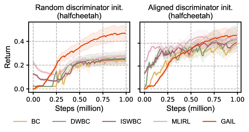
Figure 1: Effect of discriminator alignment. The curves depict the performance of GAIL’s online finetuning using the initial policies pretrained with different offline IL methods, except for the red curve representing running GAIL from scratch. In the left plot, the GAILs are provided with randomly initialized discriminators; in the right plot, they are given the discriminators approximately aligned with the pretrained policies.

Yet, achieving effective offline-to-online IL is non-trivial. It has been recognized that pretraining with BC hardly improves the performance of online IL (Sasaki et al., 2019; Jena et al., 2021; Orsini et al., 2021; Watson et al., 2024). In fact, besides BC, other offline IL methods may encounter the same issue. In Fig. 1 (left), we depict the finetuning performance of a variety of recent offline IL methods, including DWBC (Xu et al., 2022a), MLIRL (Zeng et al., 2023), and ISWBC (Li et al., 2023b) (see Section G.3.8 for the setup and results on more tasks). Albeit with improved offline IL performance, all these methods suffer performance degradation at the initial stage of finetuning. The underlying rationale of this phenomenon is that the initial discriminator of GAIL operates randomly and mismatches the warm-start policy, thus steering an erroneous policy optimization and inducing the policy to unlearn previous knowledge. To substantiate this claim, we sample more than 100 trajectories by rolling out initial policies in environments, based on which we update initial discriminators sufficiently before finetuning. As shown in Fig. 1 (right), it remedies this issue.

Unfortunately, this Monte Carlo method requires extensive number of sampled trajectories to estimate the policy’s stationary distribution, which is prohibitively expensive. Therefore, we ask: can we obtain the aligned discriminator more efficiently without repetitive Monte Carlo sampling?

5 Offline-To-Online Imitation Learning

In this section, we address the question raised in Section 4 via introducing a principled offline IL method. It can fully utilize both expert and suboptimal data ($\mathcal{D}_{e},\mathcal{D}_{s}$) to learn a near-expert offline policy that enjoys minimal discrepancy with the expert state-action distribution. More importantly, after obtaining the learned policy, our method can cleverly deduce the discriminator aligned with this policy with no additional computation or environmental interaction. Next, we begin by formally introducing the IL formulation and transforming it to an equivalent form that incorporates suboptimal data and can be optimized entirely offline.

5.1 A Surrogate Objective for Offline IL

The objective of IL can be formulated as minimizing the reverse KL-divergence between $\tilde{\rho}^{e}$ and the stationary distributions of $\pi$ (Fu et al., 2018; Kostrikov et al., 2020):

$$\min_{\pi}D_{\mathrm{KL}}(\rho^{\pi}\|\tilde{\rho}^{e})=\mathbb{E}_{(s,a)\sim\rho^{\pi}}\left[\log\frac{\rho^{\pi}(s,a)}{\tilde{\rho}^{e}(s,a)}\right].$$ (4)

Directly dealing with Problem (4) hardly exploits supplementary data like Kostrikov et al. (2020). Hence, we revert the objective to a surrogate form that incorporates $\mathcal{D}_{s}$:

$$\max_{\pi}\mathbb{E}_{(s,a)\sim\rho^{\pi}}\big{[}\tilde{R}(s,a)\big{]}-D_{\mathrm{KL}}(\rho^{\pi}\|\tilde{\rho}^{o})$$ (5)

where $\tilde{R}(s,a)\doteq\log\frac{\tilde{\rho}^{e}(s,a)}{\tilde{\rho}^{o}(s,a)}$ serves as an auxiliary reward function. The equivalence of Eqs. 4 and 5 can be easily seen via adding and subtracting $\mathbb{E}_{\rho^{\pi}}[\log\tilde{\rho}^{o}(s,a)]$ to Eq. 4. Notably, the integration of $\tilde{\rho}^{o}$ here is not trivial, and later in Section 5.3, we will show that it enables effective utilization of dynamics information within the supplementary data.

Remark 5.1.

While KL-regularized problems have been studied in the fields of RL (Nachum et al., 2019b), offline RL (Lee et al., 2022), and offline IL (Kim et al., 2022b), these solutions either require online interactions or suffer from biased gradient estimates, not sufficing guaranteed performance in offline IL (see Appendix A for details).

5.2 Auxiliary Reward Function

Before delving into Problem (5), we first describe how to calculate the auxiliary reward function in terms of the density ratio. In the low-dimensional tabular setting, we can directly compute $\tilde{\rho}^{e}(s,a)$ and $\tilde{\rho}^{o}(s,a)$ via the corresponding state-action counts in $\mathcal{D}_{e}$ and $\mathcal{D}_{o}$. However, in high-dimensional or continuous domains, estimating the densities separately and then calculating their ratio hardly works well due to error accumulation. An alternative is to estimate the log ratio via learning a discriminator $d^{*}\mathrel{\mathop{\mathchar 58\relax}}\mathcal{S}\times\mathcal{A}\rightarrow(0,1)$:

$$\max_{d}\mathbb{E}_{\tilde{\rho}^{e}}\big{[}\log d(s,a)\big{]}+\mathbb{E}_{\tilde{\rho}^{o}}\big{[}\log(1-d(s,a))\big{]}$$ (6)

where the optimal discriminator $d^{*}$ can recover

$$\tilde{R}(s,a)=\log\frac{\tilde{\rho}^{e}(s,a)}{\tilde{\rho}^{o}(s,a)}=\log\frac{d^{*}(s,a)}{1-d^{*}(s,a)}.$$ (7)

In particular, $d^{*}$ also plays an important role during online finetuning (Section 5.5).

5.3 Optimizing the Surrogate Problem

We proceed to derive the resolution of Problem (5) that can operate entirely offline without bias. Define the set of stationary distributions satisfying Bellman flow constraints:

$$\mathcal{Z}\doteq\left\{\rho\mathrel{\mathop{\mathchar 58\relax}}\rho(s,a)\geq 0,~{}f_{s}(\rho)=0,~{}\forall s\in\mathcal{S},a\in\mathcal{A}\right\}$$ (8)

where $f_{s}(\rho)\doteq(1-\gamma)\mu(s)+\gamma\sum_{a,s^{\prime}}T(s|s^{\prime},a)\rho(s^{\prime},a)-\sum_{a}\rho(s,a)$. An elementary result has shown that there exists a one-to-one correspondence between the policy and its stationary state-action distribution: if $\rho\in\mathcal{Z}$, then $\rho$ is the occupancy for policy $\pi_{\rho}(a|s)\doteq\rho(s,a)/\sum_{a^{\prime}}\rho(s,a^{\prime})$; and $\pi_{\rho}$ is the only stationary policy with $\rho$ (Syed et al., 2008, Theorem 2). Therefore, Problem (5) can be equivalently written as the following form:

$$\max_{\rho\geq 0}~{} \mathbb{E}_{(s,a)\sim\rho}\big{[}\tilde{R}(s,a)\big{]}-D_{\mathrm{KL}}(\rho\|\tilde{\rho}^{o})$$ (9)

$$\mathrm{s.t.}~{} f_{s}(\rho)=0,~{}\forall s\in\mathcal{S}.$$ (10)

Since the objective and constraints are concave and affine on $\rho$ respectively, Problem (9)–(10) is a convex optimization problem. Consider the Lagrangian of the above problem:

$$L(\rho,\nu)\doteq\; \mathbb{E}_{s,a\sim\rho}[\tilde{R}(s,a)]-D_{\mathrm{KL}}(\rho\|\tilde{\rho}^{o})+\sum_{s}\nu(s)f_{s}(\rho)$$

with $\nu$ the Lagrangian multiplier. Rearranging terms and plugging $D_{\mathrm{KL}}(\rho\|\tilde{\rho}^{o})=\sum_{s,a}\rho(s,a)\log(\rho(s,a)/\tilde{\rho}^{o}(s,a))$ in the Lagrangian, we obtain

$$L(\rho,\nu)=\; \sum_{s,a}\rho(s,a)\bigg{(}\delta_{\nu}(s,a)-\log\frac{\rho(s,a)}{\tilde{\rho}^{o}(s,a)}\bigg{)}$$

$$+(1-\gamma)\sum_{s}\nu(s)\mu(s)$$ (11)

where $\delta_{\nu}(s,a)\doteq\tilde{R}(s,a)+\gamma\sum_{s^{\prime}}\nu(s^{\prime})T(s^{\prime}|s,a)-\nu(s)$ (informally, it can be considered as an advantage function with $\nu$ treated as the value function). There always exists $\rho$ such that $\rho(s,a)>0$ for every $s\in\mathcal{S},a\in\mathcal{A}$ when each $s\in\mathcal{S}$ is reachable under the MDP $M$. From Slater’s condition, the strong duality holds. To find optimal $\rho$, we take the derivative of $L$ w.r.t. $\rho(s,a)$:

$$\frac{\partial L}{\partial\rho(s,a)}=\delta_{\nu}(s,a)-\log\frac{\rho(s,a)}{\tilde{\rho}^{o}(s,a)}-1.$$ (12)

Taking $\frac{\partial L}{\partial\rho(s,a)}=0$ yields

$$\rho(s,a)=\tilde{\rho}^{o}(s,a)\exp\left(\delta_{\nu}(s,a)-1\right).$$ (13)

Substituting Eq. 13 in Section 5.3, we obtain the dual problem (slightly abusing notation $L$) as follows:

$$\min_{\nu}L(\nu)\doteq\; \mathbb{E}_{(s,a)\sim\tilde{\rho}^{o}}\left[\exp\big{(}\delta_{\nu}(s,a)-1\big{)}\right]$$

$$+(1-\gamma)\mathbb{E}_{s\sim\mu}\left[\nu(s)\right].$$ (14)

It can be proved that $L(\nu)$ is convex on $\nu$ (see Appendix B). However, it is problematic to directly optimize Problem (5.3), because the expectation in $\delta_{\nu}$ leads to biased stochastic gradients due to double sampling, and the exponential term in Problem (5.3) easily causes numerical instability in practice.

Next, we overcome this limitation via convex conjugate.

Definition 5.2 (Convex conjugate).

For an extended real-value function $f\mathrel{\mathop{\mathchar 58\relax}}\mathbb{R}\rightarrow[-\infty,\infty]$, its conjugate is defined by $f^{*}(y)\doteq\max_{x}yx-f(x)$.

From the definition, letting $f(x)=\exp(x-1)$, its conjugate can be expressed as

$$f^{*}(y)=\max_{x}yx-\exp(x-1)=y\log y.$$ (15)

From (Bertsekas et al., 2003, Proposition 7.1.1), for any closed, proper and convex function $f$, the conjugate of the conjugate of $f$ is again $f$, i.e., $f^{**}=f$. Replacing $x$ with $\delta_{\nu}(s,a)$, we have

$$\exp\left(\delta_{\nu}(s,a)-1\right)= \max_{y(s,a)}\delta_{\nu}(s,a)y(s,a)$$

$$-y(s,a)\log y(s,a)\big{.}$$ (16)

Plugging Section 5.3 in Problem (5.3) and rearranging terms, the dual problem is equivalent to a min-max problem:

$$\min_{\nu}\max_{y}\; F(\nu,y)\doteq\mathbb{E}_{(s,a)\sim\tilde{\rho}^{o}}\big{[}\delta_{\nu}(s,a)y(s,a)-y(s,a)$$

$$\cdot\log y(s,a)\big{]}+(1-\gamma)\mathbb{E}_{s\sim\mu}[\nu(s)].$$ (17)

Since $F(\cdot,y)$ is convex with fixed $y$, and $F(\nu,\cdot)$ is concave with fixed $\nu$, the minimax theorem holds (Du & Pardalos, 1995), and Problem (5.3) is in fact a convex-concave Stochastic Saddle Point (SSP) problem. For a transition $(s,a,s^{\prime})$, denote $\tilde{\delta}_{\nu}(s,a,s^{\prime})$ as

$$\tilde{\delta}_{\nu}(s,a,s^{\prime})\doteq\tilde{R}(s,a)+\gamma\nu(s^{\prime})-\nu(s).$$ (18)

Thus, we obtain the unbiased counterpart of Problem (5.3):

$$\min_{\nu}\max_{y}\tilde{F}(\nu,y)\doteq\mathbb{E}_{(s,a,s^{\prime})\sim\mathcal{D}_{o}}\big{[}\tilde{\delta}_{\nu}(s,a,s^{\prime})y(s,a)$$

$$-y(s,a)\log y(s,a)\big{]}+(1-\gamma)\mathbb{E}_{s\sim\mathcal{D}_{o}(s_{0})}[\nu(s)].$$ (19)

Remark 5.3.

Problem (5.3) is well-suited for practical computation. First, unbiased estimates of both the objective and its gradients are easy to compute using transition samples. Second, it can be shown that Problem (5.3) enjoys a convergence rate of $O(1/\epsilon)$ in terms of the duality gap (by Nemirovski’s mirror-prox algorithm) (Nemirovski, 2004) and a finite-sample generalization bound of $O(1/\sqrt{n_{e}+n_{s}})$ under mild assumptions (Zhang et al., 2021). More importantly, the optimum of $y$ can be directly used for offline policy extraction as well as the follow-up computation of the discriminator initialization (see Sections 5.4 and 5.5).

Remark 5.4.

How to extract useful information from imperfect data remains an open problem in offline IL. In contrast to existing works that fit a world model (Yue et al., 2023; Zeng et al., 2023) or shift the prime objective (Kim et al., 2022b; Xu et al., 2022a) (see Appendix A), Problem (5.3) enables effective utilization of dynamics information within $\mathcal{D}_{e},\mathcal{D}_{s}$ in a entirely offline, model-free, and unbiased manner, achieving a correct exploitation of suboptimal data and a mitigation of the covariate shift.

5.4 Offline Policy Extraction

From Eq. 13, given optimal $\nu^{*}$, optimal $\rho^{*}$ is expressed as

$$\rho^{*}(s,a)=\tilde{\rho}^{o}(s,a)\exp\left(\delta_{\nu^{*}}(s,a)-1\right).$$ (20)

Based on Syed et al. (2008, Theorem 2), the corresponding policy of $\rho^{*}$ satisfies

$$\pi^{*}(a|s)=\frac{\rho^{*}(s,a)}{\sum_{a^{\prime}}\rho^{*}(s,a^{\prime})}\propto\tilde{\rho}^{o}(s,a)\exp\left(\delta_{\nu^{*}}(s,a)-1\right).$$ (21)

From Section 5.3, direct calculating $\delta_{\nu^{*}}(s,a)$ involves estimating an advantage-like function and can result in much additional computation. Fortunately, taking $\frac{\partial F}{\partial y(s,a)}=0$, we immediately obtain

$$y^{*}(s,a)=\exp(\delta_{\nu^{*}}(s,a)-1)$$ (22)

where $y^{*}$ is the optimum (saddle point) of Section 5.3. Therefore, we can sidestep fitting $\delta_{\nu^{*}}(s,a)$ and calculate the optimal policy directly from

$$\pi^{*}(a|s)=\frac{\tilde{\rho}^{o}(s,a)y^{*}(s,a)}{z(s)}$$ (23)

where $z$ is the partition function. We provide two options to extract the policy.

1) Reverse KL-divergence. From Eq. 7, denote $q(s,a)$ as

$$q(s,a)\doteq\tilde{\rho}^{e}(s,a)y^{*}(s,a)\left(\frac{1}{d^{*}(s,a)}-1\right).$$ (24)

Similarly to SAC (Haarnoja et al., 2018), we can learn the policy via solving the following reverse KL-divergence:

$$\min_{\pi}J(\pi)=\mathbb{E}_{s\sim\mathcal{D}_{o}}\bigg{[}D_{\mathrm{KL}}\bigg{(}\pi(\cdot|s)\,\bigg{\|}\,\frac{q(s,\cdot)}{z(s)}\bigg{)}\bigg{]}$$ (25)

which can be optimized via reparametrization in practice.

2) Forward KL-divergence. Consider the following forward KL-divergence between $\pi^{*}$ and the learning policy:

$$\mathbb{E}_{s\sim\rho^{*}}\left[D_{\mathrm{KL}}(\pi^{*}(\cdot|s)\|\pi(\cdot|s))\right]$$

$$=\; \mathbb{E}_{s\sim\rho^{*}}\left[\mathbb{E}_{a\sim\pi^{*}(\cdot|s)}\left[\log\pi^{*}(a|s)-\log\pi(a|s)\right]\right]$$

$$\Leftrightarrow\; \mathbb{E}_{(s,a)\sim\rho^{*}}\left[-\log\pi(a|s)\right]$$

$$=\; \mathbb{E}_{(s,a)\sim\tilde{\rho}^{o}}\left[-\frac{\rho^{*}(s,a)}{\tilde{\rho}^{o}(s,a)}\log\pi(a|s)\right]$$ (26)

where we omit $\mathbb{E}_{(s,a)\sim\rho^{*}}[\log\pi^{*}(a|s)]$ due to its independency to $\pi$. From Eqs. 20 and 22, the importance weight in Section 5.4 can be computed as

$$\frac{\rho^{*}(s,a)}{\tilde{\rho}^{o}(s,a)}=\exp\left(\delta_{\nu^{*}}(s,a)-1\right)=y^{*}(s,a).$$ (27)

Substituting Eq. 27 in Section 5.4, we can extract the policy via the following weighted behavior cloning:

$$\max_{\pi}J(\pi)=\mathbb{E}_{(s,a)\sim\mathcal{D}_{o}}\left[y^{*}(s,a)\log\pi(a|s)\right]$$ (28)

If we consider $\delta_{\nu^{*}}$ as an advantage function, the instantiation is consistent with the offline RL method, MARWIL (Wang et al., 2018). In addition, a keen reader may find the form of Eq. 28 bears a resemblance to DemoDICE (Kim et al., 2022b) and ISWBC (Li et al., 2023b). We elaborate on their fundamental difference in Appendix A.

5.5 Aligned Discriminator

Now, we obtain a near-expert offline policy $\pi^{*}$. As mentioned earlier, effective fintuning for an offline policy necessitates a well-aligned discriminator which is often data-hungry. However, surprisingly, we find that the discriminator for $\pi^{*}$ can be directly deduced from the components we have already obtained! Specifically, from Eq. 3, the discriminator for $\pi^{*}$ in GAIL can be expressed as

$$D_{0}(s,a)\doteq\frac{\rho^{*}(s,a)}{\rho^{*}(s,a)+\tilde{\rho}^{e}(s,a)}=\left(1+\frac{\tilde{\rho}^{e}(s,a)}{\rho^{*}(s,a)}\right)^{-1}$$ (29)

with $\rho^{*}$ defined in Eq. 13. From Eqs. 7, 20 and 22,

$$D_{0}(s,a) =\left(1+\frac{\tilde{\rho}^{e}(s,a)}{\tilde{\rho}^{o}(s,a)}\cdot\frac{\tilde{\rho}^{o}(s,a)}{\rho^{*}(s,a)}\right)^{-1}$$

$$=\left(1+\frac{d^{*}(s,a)}{1-d^{*}(s,a)}\cdot\frac{1}{\exp\left(\delta_{\nu^{*}}(s,a)-1\right)}\right)^{-1}$$

$$=\left(1+\frac{d^{*}(s,a)}{1-d^{*}(s,a)}\cdot\frac{1}{y^{*}(s,a)}\right)^{-1}.$$ (30)

Therefore, discriminator aligned with $\pi^{*}$ can be elegantly derived by simply stitching $d^{*}$ and $y^{*}$, both of which are already accessible from the pretraining phase, with no additional computation or data collection!

5.6 Implementation with Function Approximation

In practical high-dimensional and continuous domain, we use function approximation for $d$, $\nu$, $y$, and $\pi$, parameterized by $\phi_{d}$, $\phi_{\nu}$, $\phi_{y}$, and $\theta$, respectively. We solve the minimax problem (5.3) by approximating dual descent, which converges under convexity assumptions (Boyd & Vandenberghe, 2004) and works very well in the case of nonlinear function approximators (see Section G.3.4). We employ the forward policy extraction in experiments (a comparison of forward and reverse updating is included in Section G.3.7). During online finetuning, we build the initial discriminator by connecting the parameters of $\phi_{d}$ and $\phi_{y}$ learned offline:

$$D_{\phi_{y},\phi_{d}}(s,a)=\left(1+\frac{\phi_{d}(s,a)}{1-\phi_{d}(s,a)}\cdot\frac{1}{\phi_{y}(s,a)}\right)^{-1}.$$ (31)

Algorithm 1 Offline-to-online imitation learning (OLLIE)

1:  Initialize parameters $\phi_{d}$, $\phi_{\nu}$, $\phi_{y}$, and $\theta$

2:  // Offline phase

3:  Estimate reward function $\tilde{R}$ via Eqs. 6 and 7

4:  for $i=1$ to $n$ do

5:     $\phi_{\nu}\leftarrow\phi_{\nu}-\eta_{\nu}\tilde{\nabla}_{\phi_{\nu}}\tilde{F}(\phi_{\nu},\phi_{y})$

6:     $\phi_{y}\leftarrow\phi_{y}+\eta_{y}\tilde{\nabla}_{\phi_{y}}\tilde{F}(\phi_{\nu},\phi_{y})$

7:  end for

8:  for $i=1$ to $n^{\prime}$ do

9:     $\theta\leftarrow\theta-\eta_{\pi}\tilde{\nabla}J(\pi_{\theta})$

10:  end for

11:  // Online phase

12:  Initialize discriminator $D_{\phi_{y},\phi_{d}}(s,a)$ by Eq. 31

13:  Run GAIL to update $\pi_{\theta}$ and $D_{\phi_{y},\phi_{d}}(s,a)$

Then, we use a standard implementation of GAIL to continue training the policy and discriminator in the environment. We term our proposed method OffLine-to-onLine Imitation lEarning (OLLIE). The pseudocode is outlined in Algorithm 1, where $\tilde{\nabla}$ denotes the batch gradient.

6 Extensions

In this section, we first extend our method to reward scaling that can be exploited to stabilize training by ensuring the auxiliary rewards with lower variance (Rafailov et al., 2023; Fu et al., 2020). Subsequently, we generalize our method to undiscounted cases, followed by a discussion on a byproduct for offline RL. For ease of exposition, this section overloads some notations like $\delta_{\nu}$ when clear from the context.

Reward scaling. For ${\alpha}>0,\beta\geq 0$, consider the reward is scaled by $\tilde{R}_{\alpha}(s,a)\doteq{\alpha}\tilde{R}(s,a)+\beta$. Using analogous derivation from Eq. 9 to Section 5.3 – building the Lagrangian and exploiting convex conjugate to transform the dual problem – we can deduce the following minimax problem:

$$\min_{\nu}\max_{y}\; {\alpha}\mathbb{E}_{(s,a)\sim\tilde{\rho}^{o}}\big{[}\delta_{\nu}(s,a)y(s,a)-{\alpha}\log({\alpha}y(s,a))$$

$$\cdot y(s,a)\big{]}+(1-\gamma)\mathbb{E}_{s\sim\mu}\left[\nu(s)\right]$$ (32)

where $\delta_{\nu}(s,a)=\tilde{R}_{\alpha}(s,a)+\gamma\sum_{s^{\prime}}\nu(s^{\prime})T(s^{\prime}|s,a)-\nu(s)$. Similarly to Eqs. (13)–(23), the offline policy still follows Eq. 23. Based on Section 5.5, the discriminator of $\pi^{*}$ satisfies

$$D_{0}(s,a)=\left(1+\frac{d^{*}(s,a)}{1-d^{*}(s,a)}\cdot\frac{1}{{\alpha}y^{*}(s,a)}\right)^{-1}.$$ (33)

The detailed derivation can be found in Appendix C.

Undiscounted case. In the undiscounted case where $\gamma=1$, the stationary distribution is expressed as

$$\rho^{\pi}(s,a)=\lim_{H\rightarrow\infty}\frac{1}{H}\sum^{H-1}_{h=0}\Pr(s_{h}=s,a_{h}=a\mid T,\pi,\mu)$$

which renders Problem (9)–(10) ill-posed. This can be overcome by introducing an additional normalization constraint $\sum_{s,a}\rho(s,a)=1$ to the original problem. Represent $\lambda$ as the Lagrangian multiplier for the normalization constraint. Following the same line from Eq. 9 to Section 5.3, the dual problem changes to

$$\min_{\nu,\lambda}\max_{y}\; \mathbb{E}_{(s,a)\sim\tilde{\rho}^{o}}\big{[}\delta_{\nu}(s,a)y(s,a)+\lambda y(s,a)$$

$$-y(s,a)\log y(s,a)\big{]}.$$ (34)

Accordingly, the policy and discriminator match Eqs. 23 and 5.5, respectively (see Appendix D for details).

A byproduct. Given underlying reward signal $R(s,a)$ instead of $\tilde{R}(s,a)$, Problem (5) matches a formulation of offline RL (Lee et al., 2021). Thus, our method can be directly applied to offline RL. We delve into it in Appendix E.

7 Experiment

In this section, we use experimental studies to evaluate our proposed method by answering the main questions:

1. How does it perform in offline IL and online finetuning compared to existing methods across various benchmarks, especially in high-dimensional environments?

2. How is the performance affected by factors such as the number of expert/imperfect demonstrations and the quality of imperfect data?

3. What are the effects of components like the discriminator initialization and policy extraction approaches?

Experimental details, full results, and ablations are elaborated in Appendices F, G and G.3 due to space limitation.

7.1 Experimental Setup

Environments and datasets. We run experiments with 5 domains including 21 tasks: 1) AntMaze (umaze, medium, large), 2) Adroit (pen, hammer, door, relocate), 3) MuJoCo (ant, hopper, halfcheetah, walker2d), 4) FrankaKitchen (complete, partial, undirect), 5) vision-based Robomimic (lift, can, square), and 6) vision-based MuJoCo. Specifically, the MuJoCo domain consists of 4 tasks that are popularly used to evaluate OLLIE’s basic effectiveness in offline RL/IL. The Adroit benchmarks require controlling a 24-DoF robotic hand and have narrow expert data distributions, which can demonstrate OLLIE’s capabilities in dealing with more difficult robot manipulation tasks. The AntMaze tasks require composing parts of suboptimal trajectories to form more optimal policies for reaching goals, thereby capable of evaluating OLLIE’s capability in effectively utilizing imperfect demonstrations. Analogously, results on FrankaKitchen can demonstrate the imperfection-leveraging capability of OLLIE, but the tasks are non-navigation and more challenging than AntMaze due to the need of precise long-horizon manipulation. The image-based Robomimic and Mujoco (including 7 tasks) are employed to test OLLIE’s scalability to high-dimensional environments.

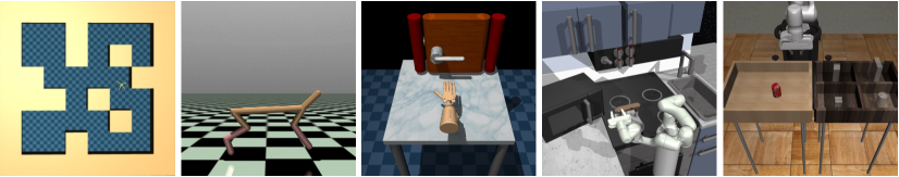
Figure 2: Benchmark environments. From left to right: AntMaze, MuJoCo, Adroit, FrankaKitchen, and vision-based Robomimic. We also consider vision-based MuJoCo with image observations.

Table 1: Normalized performance in offline IL under limited expert demonstrations and low-quality imperfect data with varying qualities. Uncertainty intervals depict standard deviation over five seeds. Expert trajectories are sampled from expert of D4RL (1 trajectory for MuJoCo and 10 for Adroit), and imperfect trajectories are sampled from the datasets listed in the second column (1000 for each task). In MuJoCo, the trajectory length is less than 1000; in Adroit, it is less than 100. The third column comprises average normalized scores of imperfect data. medium-replay and medium-expert is abbreviated to med.-rep. and med.-exp., respectively.

Task	Imperfect data	Score	BC	NBCU	CSIL	DWBC	MLIRL	ISWBC	OLLIE (ours)
ant	random	$9.2$	$-10.7\pm 11.7$	$31.1\pm 7.0$	$2.8\pm 1.3$	$24.5\pm 1.1$	$39.3\pm 9.0$	$30.4\pm 7.7$	$\bm{57.1\pm 7.0}$
	med.-rep.	$19.0$	$-10.7\pm 11.7$	$27.0\pm 6.0$	$61.0\pm 3.6$	$29.5\pm 1.3$	$57.9\pm 5.1$	$48.5\pm 3.8$	$\bm{74.2\pm 6.1}$
	medium	$80.3$	$-10.7\pm 11.7$	$45.0\pm 5.2$	$78.2\pm 8.4$	$51.6\pm 3.7$	$63.4\pm 2.5$	$59.0\pm 4.7$	$\bm{84.9\pm 2.0}$
	med.-exp.	$90.1$	$-10.7\pm 11.7$	$70.5\pm 2.0$	$100.5\pm 2.2$	$79.2\pm 8.8$	$76.1\pm 7.8$	$94.1\pm 2.7$	$\bm{123.9\pm 3.1}$
halfcheetah	random	$-0.1$	$0.2\pm 1.0$	$2.2\pm 0.1$	$22.9\pm 2.8$	$0.0\pm 0.0$	$23.8\pm 1.0$	$13.7\pm 3.0$	$\bm{35.5\pm 4.0}$
	med.-rep.	$7.3$	$0.2\pm 1.0$	$36.1\pm 5.1$	$59.9\pm 4.4$	$36.0\pm 7.5$	$77.8\pm 2.4$	$\bm{87.5\pm 3.0}$	$44.8\pm 4.1$
	medium	$40.7$	$0.2\pm 1.0$	$23.8\pm 9.0$	$62.6\pm 9.9$	$35.1\pm 9.7$	$64.3\pm 1.9$	$\bm{83.6\pm 3.2}$	$62.3\pm 4.2$
	med.-exp.	$70.3$	$0.2\pm 1.0$	$36.1\pm 15.2$	$101.6\pm 1.5$	$5.7\pm 3.3$	$89.7\pm 5.5$	$97.2\pm 1.2$	$\bm{114.3\pm 2.0}$
hopper	random	$1.2$	$17.8\pm 5.4$	$6.6\pm 3.9$	$17.1\pm 6.8$	$\bm{77.8\pm 12.7}$	$54.7\pm 16.7$	$64.7\pm 9.9$	$71.1\pm 3.5$
	med.-rep.	$6.8$	$17.8\pm 5.4$	$29.1\pm 4.2$	$28.7\pm 8.3$	$78.9\pm 2.0$	$68.5\pm 17.9$	$90.3\pm 3.1$	$\bm{101.0\pm 2.5}$
	medium	$44.1$	$17.8\pm 5.4$	$24.9\pm 14.0$	$49.3\pm 4.3$	$90.6\pm 3.0$	$68.0\pm 14.2$	$73.0\pm 7.8$	$\bm{98.7\pm 7.0}$
	med.-exp.	$72.0$	$17.8\pm 5.4$	$\bm{111.7\pm 1.3}$	$96.7\pm 3.6$	$100.8\pm 2.1$	$95.0\pm 6.0$	$97.6\pm 1.6$	$108.5\pm 1.7$
walker2d	random	$0.0$	$4.6\pm 3.9$	$0.0\pm 0.0$	$8.1\pm 5.6$	$56.9\pm 11.6$	$49.9\pm 6.7$	$48.2\pm 4.7$	$\bm{59.8\pm 8.5}$
	med.-rep.	$13.0$	$4.6\pm 3.9$	$7.4\pm 5.0$	$27.6\pm 4.3$	$53.7\pm 4.6$	$67.6\pm 7.2$	$69.5\pm 3.2$	$\bm{79.0\pm 2.3}$
	medium	$62.0$	$4.6\pm 3.9$	$23.9\pm 2.7$	$92.9\pm 3.7$	$67.0\pm 7.8$	$78.5\pm 5.5$	$56.0\pm 8.0$	$\bm{111.7\pm 0.9}$
	med.-exp.	$81.0$	$4.6\pm 3.9$	$11.6\pm 8.4$	$99.5\pm 2.7$	$92.6\pm 5.4$	$90.0\pm 7.8$	$88.0\pm 3.5$	$\bm{120.2\pm 4.4}$
hammer	human	$2.7$	$5.7\pm 6.8$	$0.0\pm 0.0$	$16.7\pm 8.9$	$6.6\pm 8.3$	$1.0\pm 0.1$	$6.5\pm 5.1$	$\bm{46.1\pm 6.5}$
	clone	$0.5$	$5.7\pm 6.8$	$0.3\pm 0.1$	$14.2\pm 5.6$	$3.3\pm 2.8$	$1.6\pm 1.0$	$2.8\pm 2.3$	$\bm{51.5\pm 4.4}$
pen	human	$2.1$	$40.3\pm 10.3$	$3.2\pm 9.8$	$39.0\pm 5.6$	$42.8\pm 19.3$	$18.7\pm 2.6$	$49.5\pm 2.9$	$\bm{67.4\pm 5.6}$
	clone	$59.9$	$40.3\pm 10.3$	$1.0\pm 1.0$	$45.6\pm 4.7$	$48.0\pm 3.9$	$23.4\pm 1.5$	$51.3\pm 6.9$	$\bm{68.0\pm 1.6}$
door	human	$2.6$	$2.8\pm 3.9$	$0.0\pm 0.0$	$24.8\pm 3.6$	$0.0\pm 0.0$	$1.0\pm 0.8$	$2.9\pm 2.1$	$\bm{28.9\pm 2.9}$
	clone	$-0.1$	$2.8\pm 3.9$	$0.0\pm 0.0$	$21.6\pm 2.1$	$1.0\pm 1.0$	$1.0\pm 1.0$	$1.0\pm 1.0$	$\bm{31.9\pm 4.9}$
relocate	human	$2.3$	$0.0\pm 0.0$	$0.0\pm 0.0$	$7.7\pm 8.8$	$0.0\pm 0.0$	$1.0\pm 0.2$	$0.0\pm 0.0$	$\bm{31.2\pm 5.8}$
	clone	$-0.1$	$0.0\pm 0.0$	$0.0\pm 1.0$	$10.2\pm 4.4$	$1.0\pm 1.0$	$1.0\pm 1.0$	$1.0\pm 1.0$	$\bm{40.8\pm 6.9}$

During offline training, we use the D4RL datasets (Fu et al., 2020) for AntMaze, MuJoCo, Adroit, and FrankaKitchen and use the robomimic (Mandlekar et al., 2022) datasets for vision-based Robomimic. We construct vision-based MuJoCo datasets using the same method introduced in Fu et al. (2020). Details on environments and datasets can be found in Sections F.1 and F.2.

Baselines. We evaluate our method against four strong offline IL methods, DWBC (Xu et al., 2022a), ISWBC (Li et al., 2023b), MLIRL (Zeng et al., 2023), and CSIL (Watson et al., 2024), all of which can utilize imperfect demonstrations (see Appendices A and F.3 for more information). We also compare our method with BC and its counterpart with union offline data, termed NBCU (Li et al., 2023b).

Reproducibility. All details of our experiments are provided in the appendices in terms of the tasks, network architectures, hyperparameters, etc. We implement all baselines and environments based on open-source repositories. The code is available at https://github.com/HansenHua/OLLIE-offline-to-online-imitation-learning. Of note, our method is robust in hyperparameters, identical for all tasks except for the change of neural nets to CNNs in vision-based domains.

7.2 Experimental Results

7.2.1 Performance in Offline IL

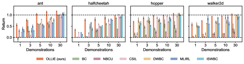
Figure 11: Performance in offline IL with varying quantities of expert trajectories in MuJoCo. Uncertainty intervals depict standard deviation over five seeds. OLLIE uses fewer expert demonstrations to attain expert performance, demonstrating its great demonstration efficiency compared to existing methods.

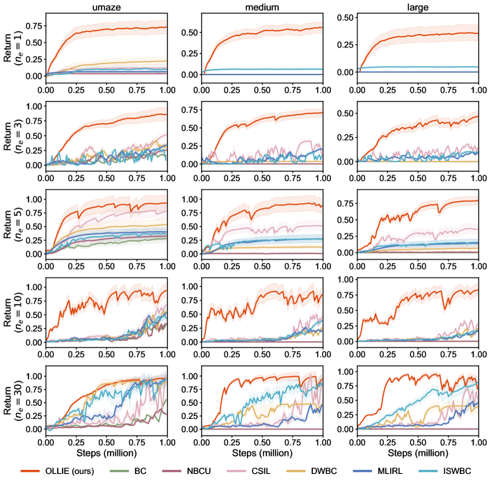
Figure 16: Learning curves in offline IL with varying quantities of expert trajectories in AntMaze. Uncertainty intervals depict standard deviation over five seeds. $n_{e}$ represents expert trajectories. OLLIE consistently and significantly surpasses existing methods in terms of convergence speed and stability.

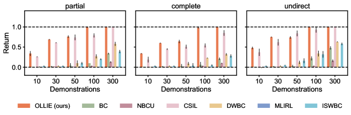
Figure 17: Performance in offline IL with varying quantities of expert trajectories in FrankaKitchen. Uncertainty intervals depict standard deviation over five seeds. OLLIE uses fewer expert demonstrations to attain expert performance, demonstrating its great demonstration efficiency in comparison with existing methods.

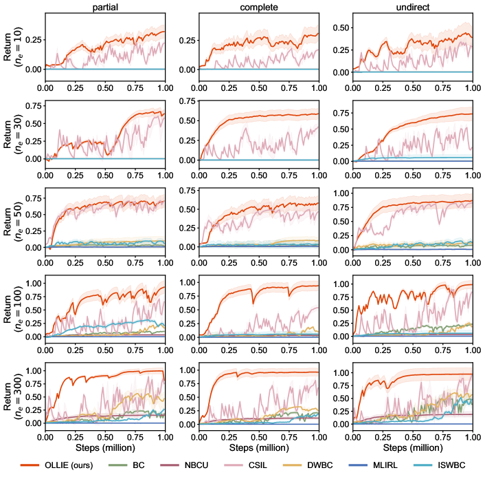
Figure 18: Learning curves in offline IL with varying quantities of expert trajectories in FrankaKitchen. Uncertainty intervals depict standard deviation over five seeds. $n_{e}$ represents expert trajectories. OLLIE consistently exhibits fast and stabilized convergence. CSIL also works well in this domain.

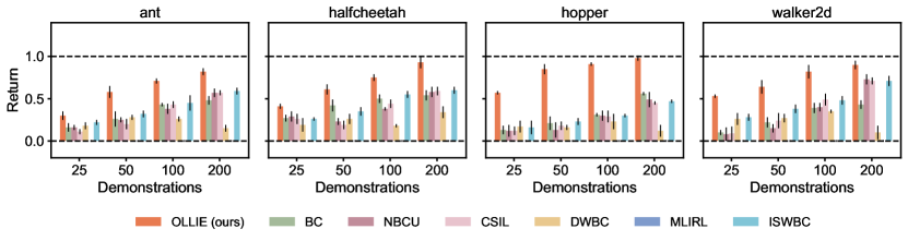
Figure 19: Performance in offline IL with varying quantities of expert trajectories in vision-based MuJoCo. Uncertainty intervals depict standard deviation over five seeds. OLLIE uses much fewer expert demonstrations to attain expert performance, demonstrating its great demonstration efficiency in high-dimensional environments.

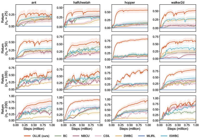
Figure 20: Learning curves in offline IL with varying quantities of expert trajectories in vision-based MuJoCo. Uncertainty intervals depict standard deviation over five seeds. $n_{e}$ represents expert trajectories. OLLIE consistently and significantly surpasses existing methods in terms of convergence speed and stability.

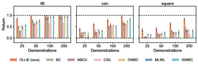
Figure 21: Performance in offline IL with varying quantities of expert trajectories in vision-based Robomimic. Uncertainty intervals depict standard deviation over five seeds. OLLIE uses much fewer expert demonstrations to attain expert performance, demonstrating its great demonstration efficiency in high-dimensional environments.

We evaluate OLLIE’s performance in offline IL across all benchmark environments, with 1000 sampled imperfect trajectories and varying numbers of expert trajectories (ranging from 1 to 30 in AntMaze and MuJuCo, from 10 to 300 in Adroit and FrankaKitchen, and from 25 to 200 in vision-based MuJoCo and Robomimic). The employed datasets can be found in Table 4. We present two selected results in Fig. 3 and provide full results in Section G.1.1. OLLIE consistently and significantly outperforms existing methods in terms of performance, convergence speed, and demonstration efficiency, especially in challenging robotic manipulation and vision-based domains. For example, with limited expert data, OLLIE outperforms baseline methods often by 2-4x and converges often within 0.2m steps (Figs. 11, 12, 15, 16, 13, 14, 17, 18, 19, 20, 21 and 22).

We also run experiments with different qualities of imperfect data. As showcased in Table 1, OLLIE surpasses the baselines in 20/24 settings by wide margins, corroborating its robustness and superiority in offline IL. Learning curves are provided in Section G.1.2.

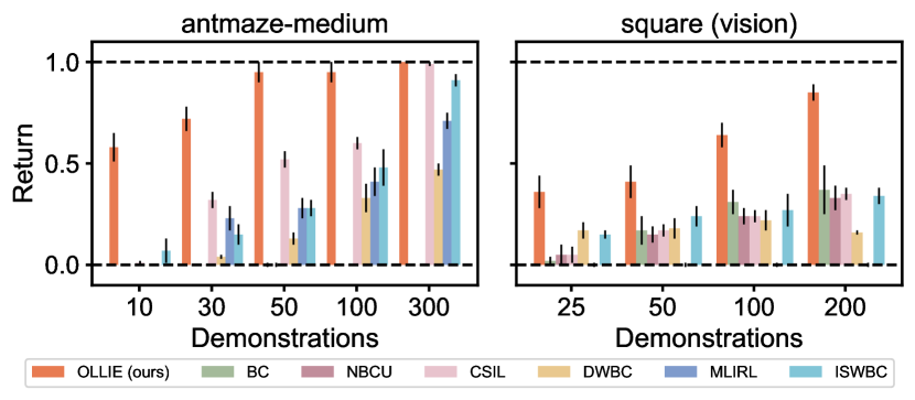
Figure 3: Comparative performance in offline IL with varying expert demonstrations. The scores are normalized and averaged over 5 seeds with standard deviation depicted by uncertainty intervals.

7.2.2 Performance in Online Fintuning

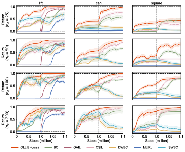
Figure 36: End-to-end learning curves from offline pretraining to online finetuning under varying quantities of expert trajectories in vision-based Romomimic. Uncertainty intervals depict standard deviation over five seeds. $n_{e}$ represents expert trajectories. $n_{e}$ represents expert trajectories. The simple combination of existing offline IL and GAIL suffers from unlearning pretrained knowledge. OLLIE not only avoids this issue but also expedites online training. This is attributed to OLLIE’s initial discriminator aligning with the well-performed policy initialization, thereby acting as a good local reward function capable of guiding fast policy search. The results reveal OLLIE’s potential in practical, high-dimensional scenarios. In addition, analogously to AntMaze, GAIL from scratch proves unsuccessful even with sufficient expert demonstrations in can and square, which implies the importance of effective pretraining in IL.

After obtaining pretrained policies, we examine the finetuning performance under different quantities of expert demonstrations. Fig. 4 showcases two selected results, and Section G.2 includes comprehensive results for all tasks. We find OLLIE not only avoids the unlearning phenomenon but also hastens online training. For example, as demonstrated in Fig. 4 (right), OLLIE improves the offline performance by 2x with fewer than 10 environmental episodes. Importantly, even in challenging tasks like vision-based can and square where GAIL from scratch fails (Fig. 36), OLLIE performs well. This underscores the significance of effective pretraining in the context of IL.

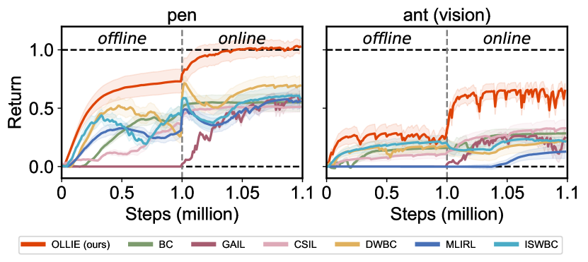
Figure 4: End-to-end performance from offline pretraining to online finetuning. The results are normalized and averaged over 5 seeds with standard deviation depicted by uncertainty intervals.

8 Limitation and Discussion

In this paper, we study offline-to-online IL that pretrains a good policy initialization, followed by online finetuning with minimal interaction. First, we derive a surrogate objective for standard IL, of which the dual problem is convex. Then, we employ the convex conjugate to transform the dual problem into a convex-concave SSP that can be optimized with unbiased stochastic gradients in an entirely offline fashion. Importantly, the transformation enables us to directly extract the optimal policy using weighted behavior cloning and deduce its corresponding discriminator which can be seamlessly used in GAIL to achieve continual learning. We believe our method can benefit many real-world domains including robotics, autonomous driving, and foundation model training where designing a reward function is challenging, while environmental interaction is necessary yet costly.

A limitation of OLLIE is the GAIL-based finetuning. The on-policy and adversarial nature of GAIL may lead to sample inefficiency and training instability in some scenarios. An avenue for future work is to render OLLIE compatible with non-adversarial or off-policy IL methods. In addition, OLLIE’s connection with offline RL suggests there is scope to bridge offline IL and offline RL. Another future direction is to explore the best utilization of unlabeled data in offline RL with the aid of IL.

Impact Statement

This paper presents work whose goal is to advance the field of Reinforcement Learning. There are many potential societal consequences of our work, none which we feel must be specifically highlighted here.

Appendix A Related Work (Extended)

In this section, we discuss recent relevant literature in detail. We shed more light on the differences and strengths of the proposed methods in comparison with the existing offline IL counterparts.

A.1 Online Imitation Learning

Imitation learning has a long history (see Osa et al. (2018); Arora & Doshi (2021) for comprehensive overviews). Classical IL methods often cast IL as IRL to improve the efficiency in utilization of expert demonstrations (Russell, 1998; Ng & Russell, 2000; Abbeel & Ng, 2004; Ratliff et al., 2006; Syed & Schapire, 2007; Ziebart et al., 2008; Levine et al., 2010, 2011; Choi & Kim, 2013). Yet, these methods are computationally prohibitive because they require repetitively running RL as intermediate steps. In the seminal work (Ho & Ermon, 2016), the authors introduce GAIL that circumvents the inner-loop RL via building the connection between IL and GAN (Goodfellow et al., 2014). It trains a discriminator network to distinguish between the state-actions ‘generated’ by the expert and the learning policy; the discriminator in turn acts as a local reward function guiding the policy to take expert behaviors. GAIL and its follow-up AIL works (Li et al., 2017; Fu et al., 2018; Kostrikov et al., 2018; Blondé & Kalousis, 2019; Sasaki et al., 2019; Wang et al., 2019; Barde et al., 2020; Ghasemipour et al., 2020; Ke et al., 2021; Ni et al., 2021; Swamy et al., 2021a; Viano et al., 2022; Al-Hafez et al., 2023) have been proven particularly successful from low-dimensional continuous control to complex and high-dimensional domains like autonomous driving from raw pixels as input (Kuefler et al., 2017; Zou et al., 2018; Ding et al., 2019; Arora & Doshi, 2021; Jena et al., 2021). In theory, Chen et al. (2019); Zhang et al. (2020); Guan et al. (2021) establish guarantees for GAIL in terms of global convergence and generalization. However, the AIL methods are typically resource-intensive as they require sampling a large number of trajectories during training to approximate the stationary distribution of the learning policy. This nature is inherently risky and costly, particularly in the initial stage where the policy performs randomly, thereby precluding the use of these methods in settings where interactions with the environment are expensive and limited such as in autonomous driving and industrial processes. There is a clear need for IL methods with minimal environmental interactions.

A.2 Offline Imitation Learning

The simplest approach to offline IL is BC (Pomerleau, 1988) that directly mimics the behavior using regression, whereas it is fundamentally limited by disregarding dynamics information in the demonstration data. It is prone to covariate shift and inevitably suffers from error compounding, i.e., there is no way for the policy to learn how to recover if it deviates from the expert behavior to a state not seen in the expert demonstrations (Rajaraman et al., 2020). Considerable research has been devoted to developing new offline IL methods to remedy this problem, which can be generally divided into two categories, offline IRL and direct policy extraction. We discuss them in what follows.

Offline inverse reinforcement learning. Offline IRL aims at learning a reward function from offline datasets to comprehend and generalize the underlying intentions behind expert behaviors (Lee et al., 2019). Zolna et al. (2020) propose ORIL that constructs a reward function to discriminate expert and exploratory trajectories, followed by an offline RL progress. Chan & van der Schaar (2021) use a variational method to jointly learn an approximate posterior distribution over the reward and policy. Garg et al. (2021) simplify the AIL game-theoretic objective over policy and reward functions to an optimization over the soft $Q$-function which implicitly represents both reward and policy. Watson et al. (2024) study a problem related to this work on how to improve the BC policy using additional experience. They develop CSIL that exploits a BC policy to define an estimate of a shaped reward function that can then be used to finetune the policy using online interactions. Unfortunately, the heteroscedastic parametric reward functions have undefined values beyond the offline data manifold and easily collapse to the reward limits due to the Tanh transformation and network extrapolation. The reward extrapolation errors may induce the learned reward functions to incorrectly explain the task and misguide the agent in unseen environments (Yue et al., 2023).

To deal with this problem, recent works on offline IRL focus more on model-based methods. Chang et al. (2021) introduce MILO that uses a model uncertainty estimate to penalize the learning reward function on out-of-distribution state-actions. Yue et al. (2023) incorporate an additional conservatism term to the MaxEnt IRL framework (Ziebart et al., 2008), implicitly penalizing out-of-distribution behaviors from model rollouts. Analogously, Zeng et al. (2022) propose MLIRL that can recover the reward function, whose corresponding optimal policy maximizes the likelihood of observed expert demonstrations under a learned conservative world model. However, these model-based approaches introduce additional difficulty in fitting the world model and struggle to scale in high-dimensional environments.

Direct policy extraction. Jarrett et al. (2020) propose EDM to enable sampling from an energy-based psuedo-state visitation distribution of the learning policy rather than actual online rollouts; however, it has been questioned that the psuedo-state distribution might be disconnected from the learning policy’s true state distribution (see Swamy et al. (2021b)). Sasaki & Yamashina (2021) analyze why the imitation policy trained by BC deteriorates its performance when using noisy demonstrations. They reuse an ensemble of policies learned from the previous iteration as the weight of the original BC objective to extract the expert behaviors. However, this requires that expert data occupies the majority proportion of the offline dataset, otherwise the policy will be misguided to imitate the suboptimal data. Florence et al. (2022) propose to reformulate BC using implicit models. They empirically show that it is beneficial to use a conditional energy-based model to represent the policy instead of feed-forward neural networks in the domain of robotic control. Xu et al. (2022a) introduce DWBC that exploits a crafted discriminator to distinguish the expert and imperfect data, the outputs of which weights the policy likelihood in BC, with the aim of imitating the noisy demonstrations selectively. Yet, DWBC incorporates the density of the learning policy into the input of the discriminator, losing a rigorous connection with the IL objective. Analogously, ISWBC (Li et al., 2023b) weight BC by the density ratio of empirical expert data and union offline data, whereas its performance can be guaranteed only when the offline data cover the stationary state-action distribution of the expert (Li et al., 2023b, Theorem 3), which is often impractical. In particular, although our reverse KL-regularized policy extraction in Eq. 28 is similar to the form of weighted BC, there exists a fundamental difference in the form of importance weights:

ISWBC: $$\quad\max_{\pi}\mathbb{E}_{(s,a)\sim\tilde{\rho}^{o}}\bigg{[}\frac{\color[rgb]{0,0,1}\tilde{\rho}^{e}(s,a)}{\tilde{\rho}^{o}(s,a)}\log\pi(a|s)\bigg{]}~{}\Leftrightarrow~{}\min_{\pi}\mathbb{E}_{s\sim{\color[rgb]{0,0,1}\tilde{\rho}^{e}}}\left[D_{\mathrm{KL}}({\color[rgb]{0,0,1}\tilde{\pi}^{e}(\cdot|s)}\|\pi(\cdot|s))\right]$$ (35)

OLLIE: $$\quad\max_{\pi}\mathbb{E}_{(s,a)\sim\tilde{\rho}^{o}}\bigg{[}\frac{\color[rgb]{0,0,1}\rho^{*}(s,a)}{\tilde{\rho}^{o}(s,a)}\log\pi(a|s)\bigg{]}~{}\Leftrightarrow~{}\min_{\pi}\mathbb{E}_{s\sim{\color[rgb]{0,0,1}\rho^{*}}}\left[D_{\mathrm{KL}}({\color[rgb]{0,0,1}\pi^{*}(\cdot|s)}\|\pi(\cdot|s))\right]$$ (36)

where $\tilde{\rho}^{e}$ and $\tilde{\rho}^{*}$ are the empirical expert distribution and the optimum of $\min_{\pi}D_{\mathrm{KL}}(\rho^{\pi}\|\tilde{\rho}^{*})$, respectively. It is worth noting that $\tilde{\rho}^{e}$ typically does not satisfy the Bellman flow constraint; in contrast, $\tilde{\rho}^{*}$ complies with the constraint and is thereby a real stationary state-action distribution that stays closest to the empirical expert distribution. According to Syed et al. (2008, Theorem 2), the optimal policy of Eq. 36 recovers $\tilde{\rho}^{*}$, but it is not be ensured by optimizing Eq. 35. As a consequence, ISWBC typically necessitates a relatively larger number of expert demonstrations to attain a satisfactory performance (see Appendix G).

From a technical point of view, this work bears a resemblance to the Stationary Distribution Correction (DICE) family (Nachum et al., 2019a, b; Kostrikov et al., 2020; Lee et al., 2021; Kim et al., 2022b, a; Ma et al., 2022; Yu et al., 2023). The terminology DICE is first introduced in Nachum et al. (2019a) for off-policy estimation, referring to the ratio between the state-action marginals of the learning policy and a reference policy. Their follow-up work (Nachum et al., 2019b) operates the technique in (online) policy optimization. Building on Nachum et al. (2019a), Kostrikov et al. (2020) propose ValueDICE that exploits the Donsker-Varadhan representation of KL-divergence and change of variables to transform the AIL problem (distribution matching) to an entirely off-policy objective. Since ValueDICE imitates all given demonstrations, it often requires a large amount of clean expert data, which can be expensive for real-world tasks. To deal with this issue, Kim et al. (2022b) introduce DemoDICE that incorporates an additional KL-regularization on imperfect demonstrations to enhance offline data support. However, the regularization term requires carefully weighting to avoid overfitting in imperfect data (Yu et al., 2023) and results in a biased optimization to the IL objective (Li et al., 2023b); in contrast, the surrogate objective considered in this work is equivalent to the original problem, $\min_{\pi}D_{\mathrm{KL}}(\rho^{\pi}\|\tilde{\rho}^{e})$:

$$(\texttt{DemoDICE})~{}\min_{\pi}D_{\mathrm{KL}}(\rho^{\pi}\|\tilde{\rho}^{e})+\alpha D_{\mathrm{KL}}(\rho^{\pi}\|\tilde{\rho}^{o}),\quad(\texttt{OLLIE})~{}\max_{\pi}\mathbb{E}_{(s,a)\sim\rho^{\pi}}\left[\log\frac{\tilde{\rho}^{e}(s,a)}{\tilde{\rho}^{o}(s,a)}\right]-D_{\mathrm{KL}}(\rho^{\pi}\|\tilde{\rho}^{o}).$$ (37)

Recently, Yu et al. (2023) propose RelaxDICE employ an asymmetrically-relaxed $f$-divergence instead of KL-divergence to ameliorate the potentially over conservatism of DemoDICE, whereas it still suffers from a biased objective. In addition, Kim et al. (2022a); Ma et al. (2022) study a relevant but different problem of learning from observation with no access to expert actions. Of note, while these DICE-based methods also explore the Lagrangian duality to deal with the prime problem, their induced dual problems often follow the form of ‘logarithm-expectation-exponential-expectation’ (Kostrikov et al., 2020; Kim et al., 2022b, a; Lee et al., 2021; Ma et al., 2022; Yu et al., 2023), whereby the two expectations cannot be estimated without bias from the batch of samples (Swamy et al., 2021a; Sun et al., 2021). Instead, our derived dual objective follows the convex-concave SSP, enabling an unbiased estimate and inheriting the properties of the convex-concave SSP in both methodology and theory. More importantly, the optimal auxiliary variable $y^{*}$ of the dual problem is critical in policy extraction and subsequent online finetuning.

A.3 Offline-To-Online Reinforcement Learning

The recipe of pretraining and finetuning has led to great success in many modern machine learning domains (Brown et al., 2020; He et al., 2022). Very recently, numerous efforts seek to translate such a recipe to decision-making problems, which utilizes offline RL for initializing value functions and policies from fixed datasets and subsequently uses RL to improve the initialization (Lee et al., 2022; Mark et al., 2022; Song et al., 2022; Ball et al., 2023; Li et al., 2023a; Nakamoto et al., 2023; Wagenmaker & Pacchiano, 2023; Wang et al., 2023a, b; Yang et al., 2023; Zhang & Zanette, 2023). In light of these advances, a potential solution to offline-to-online IL might be abstracting a reward function from offline, followed by adapting forward RL to further finetune the policy. However, it is inherently indirect, and the reward extrapolation would largely exacerbate the difficulty in both offline and online IL.

Appendix B Convexity of $L(\nu)$

Recall the expression of $L(\nu)$:

$$L(\nu)=(1-\gamma)\mathbb{E}_{s\sim\mu}[\nu(s)]+\mathbb{E}_{(s,a)\sim\tilde{\rho}^{o}}\Big{[}\exp\big{(}\tilde{R}(s,a)+\gamma\sum_{s^{\prime}}\nu(s^{\prime})T(s^{\prime}|s,a)-\nu(s)-1\big{)}\Big{]}.$$ (38)

For any $\nu_{1},\nu_{2}$ ($\nu_{1}\neq\nu_{2}$) and $\lambda\in(0,1)$, we have

$$L(\lambda\nu_{1}+(1-\lambda)\nu_{2})=\; \mathbb{E}_{(s,a)\sim\tilde{\rho}^{o}}\Big{[}\exp\Big{(}\tilde{R}(s,a)+\gamma\sum\nolimits_{s^{\prime}}\big{(}\lambda\nu_{1}(s^{\prime})+(1-\lambda)\nu_{2}(s^{\prime})\big{)}T(s^{\prime}|s,a)$$

$$-\big{(}\lambda\nu_{1}(s)+(1-\lambda)\nu_{2}(s)\big{)}-1\Big{)}\Big{]}+(1-\gamma)\mathbb{E}_{s\sim\mu}\big{[}\lambda\nu_{1}(s)+(1-\lambda)\nu_{2}(s)\big{]}$$

$$=\; \mathbb{E}_{(s,a)\sim\tilde{\rho}^{o}}\Big{[}\exp\Big{(}\lambda\big{(}\tilde{R}(s,a)+\gamma\sum\nolimits_{s^{\prime}}\nu_{1}(s^{\prime})T(s^{\prime}|s,a)-\nu_{1}(s)-1\big{)}$$

$$+(1-\lambda)\big{(}\tilde{R}(s,a)+\gamma\sum\nolimits_{s^{\prime}}\nu_{2}(s^{\prime})T(s^{\prime}|s,a)-\nu_{2}(s)-1\big{)}\Big{)}\Big{]}$$

$$+\lambda(1-\gamma)\mathbb{E}_{s\sim\mu}[\nu_{1}(s)]+(1-\lambda)(1-\gamma)\mathbb{E}_{s\sim\mu}[\nu_{2}(s)]$$

$$\leq\; \mathbb{E}_{(s,a)\sim\tilde{\rho}^{o}}\Big{[}\lambda\exp\big{(}\tilde{R}(s,a)+\gamma\sum\nolimits_{s^{\prime}}\nu_{1}(s^{\prime})T(s^{\prime}|s,a)-\nu_{1}(s)-1\big{)}$$

$$+(1-\lambda)\exp\big{(}\tilde{R}(s,a)+\gamma\sum\nolimits_{s^{\prime}}\nu_{2}(s^{\prime})T(s^{\prime}|s,a)-\nu_{2}(s)-1\big{)}\Big{]}$$

$$+\lambda(1-\gamma)\mathbb{E}_{s\sim\mu}[\nu_{1}(s)]+(1-\lambda)(1-\gamma)\mathbb{E}_{s\sim\mu}[\nu_{2}(s)]$$

$$=\; \lambda L(\lambda\nu_{1})+(1-\lambda)L(\nu_{2})$$ (39)

where the last inequality follows the convexity of $\exp(\cdot)$. From the definition of the convex function, we obtain the result.

Appendix C Auxiliary Reward Scaling

For ${\alpha}>0,\beta\geq 0$, consider the reward function is scaled by $\tilde{R}_{\alpha}(s,a)\doteq{\alpha}\tilde{R}(s,a)+\beta$. Problem (9)–(10) can be rewritten as

$$\max_{\rho\geq 0} ~{}\mathbb{E}_{(s,a)\sim\rho}\big{[}\tilde{R}_{\alpha}(s,a)\big{]}-{\alpha}D_{\mathrm{KL}}(\rho\|\tilde{\rho}^{o})$$ (40)

$$\mathrm{s.t.} ~{}f_{s}(\rho)=0,~{}\forall s\in\mathcal{S}.$$ (41)

The objective and constraints are concave and affine on $\rho$, and hence it is a convex optimization problem. The corresponding Lagrangian can be expressed as

$$L(\rho,\nu) =\sum_{s,a}\rho(s,a)\bigg{(}\tilde{R}_{\alpha}(s,a)+\gamma\sum_{s^{\prime}}\nu(s^{\prime})T(s^{\prime}|s,a)-\nu(s)-{\alpha}\log\frac{\rho(s,a)}{\tilde{\rho}^{o}(s,a)}\bigg{)}+(1-\gamma)\sum_{s}\nu(s)\mu(s)$$

$$=\sum_{s,a}\rho(s,a)\bigg{(}\delta_{\nu}(s,a)-{\alpha}\log\frac{\rho(s,a)}{\tilde{\rho}^{o}(s,a)}\bigg{)}+(1-\gamma)\sum_{s}\nu(s)\mu(s)$$ (42)

where $\nu$ is the Lagrangian multiplier, and $\delta_{\nu}(s,a)=\tilde{R}_{\alpha}(s,a)+\gamma\sum_{s^{\prime}}\nu(s^{\prime})T(s^{\prime}|s,a)-\nu(s)$. From the Slater’s condition, the strong duality holds. Taking derivative of $L$ w.r.t. $\rho(s,a)$, we have

$$\frac{\partial L}{\partial\rho(s,a)}=\delta_{\nu}(s,a)-{\alpha}\log\frac{\rho(s,a)}{\tilde{\rho}^{o}(s,a)}-{\alpha}.$$ (43)

Letting the derivative to 0, we can write

$$\rho(s,a)=\tilde{\rho}^{o}(s,a)\exp\left(\frac{1}{{\alpha}}\delta_{\nu}(s,a)-1\right).$$ (44)

Substituting Eq. 44 in Appendix C, we obtain the dual problem:

$$\min_{\nu}L(\nu)={\alpha}\mathbb{E}_{(s,a)\sim\tilde{\rho}^{o}}\left[\exp\left(\frac{1}{{\alpha}}\delta_{\nu}(s,a)-1\right)\right]+(1-\gamma)\mathbb{E}_{s\sim\mu}\left[\nu(s)\right].$$ (45)

Denote $f(x)\doteq\exp(ax-b)$ ($a>0,b\geq 0$). From the definition of convex conjugate, the following fact holds:

$$f^{*}(y)=\max_{x}yx-\exp(ax-b)=\left(\frac{b}{a}-\frac{1}{a}+\frac{1}{a}\log\left(\frac{1}{a}y\right)\right)y.$$ (46)

Due to the strict convexity of $f(x)$, $f^{**}=f$, thereby

$$\exp\left(\frac{1}{{\alpha}}\delta_{\nu}(s,a)-1\right)=\max_{y(s,a)}\delta_{\nu}(s,a)y(s,a)-{\alpha}\log\left({\alpha}y(s,a)\right)y(s,a).$$ (47)

Thus, the dual problem is equivalent to the following minimax problem:

$$\min_{\nu}\max_{y}F(\nu,y)={\alpha}\mathbb{E}_{(s,a)\sim\tilde{\rho}^{o}}\left[\delta_{\nu}(s,a)y(s,a)-{\alpha}\log\left({\alpha}y(s,a)\right)y(s,a)\right]+(1-\gamma)\mathbb{E}_{s\sim\mu}\left[\nu(s)\right].$$ (48)

Denote $\tilde{\delta}_{\nu}(s,a,s^{\prime})=\tilde{R}_{\alpha}(s,a)+\gamma\nu(s^{\prime})-\nu(s)$. The empirical counterpart of Eq. 48 is

$$\min_{\nu}\max_{y}\tilde{F}(\nu,y)={\alpha}\mathbb{E}_{(s,a,s^{\prime})\sim\mathcal{D}_{o}}\left[\tilde{\delta}_{\nu}(s,a,s^{\prime})y(s,a)-{\alpha}\log\left({\alpha}y(s,a)\right)y(s,a)\right]+(1-\gamma)\mathbb{E}_{s\sim\mu}\left[\nu(s)\right].$$ (49)

Taking $\frac{\partial F}{\partial y(s,a)}=0$ yields

$$\exp\left(\frac{1}{{\alpha}}\delta_{\nu^{*}}(s,a)-1\right)={\alpha}y^{*}(s,a).$$ (50)

From Eq. 44, given the optimal $\nu^{*}$, the optimal $\rho^{*}$ equals

$$\rho^{*}(s,a)=\tilde{\rho}^{o}(s,a)\exp\left(\frac{1}{{\alpha}}\delta_{\nu^{*}}(s,a)-1\right)=\alpha y^{*}(s,a)\tilde{\rho}^{o}(s,a).$$ (51)

Similarly to Eqs. (13)–(23), the offline policy still follows Eq. 23. Based on Section 5.5, the discriminator initialization changes to

$$D_{0}(s,a)=\frac{\rho^{*}(s,a)}{\rho^{*}(s,a)+\tilde{\rho}^{e}(s,a)}=\left(1+\frac{\tilde{\rho}^{e}(s,a)}{\tilde{\rho}^{o}(s,a)}\cdot\frac{\tilde{\rho}^{o}(s,a)}{\rho^{*}(s,a)}\right)^{-1}=\left(1+\frac{d^{*}(s,a)}{1-d^{*}(s,a)}\cdot\frac{1}{{\alpha}y^{*}(s,a)}\right)^{-1}.$$ (52)

Appendix D Undiscounted Case

In undiscounted case ($\gamma=1$), the stationary state-action distribution is expressed as

$$\rho^{\pi}(s,a)=\lim_{H\rightarrow\infty}\frac{1}{H}\sum^{H-1}_{h=0}\Pr(s_{h}=s,a_{h}=a\mid T,\pi,\mu).$$ (53)

It renders Problem (9)–(10) ill-posed: if $\rho^{*}$ is the optimizer to the problem, $a\rho^{*}$ is still the optimizer for any $a>0$. Building on Lee et al. (2021), it can be overcome by introducing normalization constraint $\sum_{s,a}\rho(s,a)=1$ to Problem (9)–(10). We reformulate Problem (5) as follows:

$$\max_{\rho\geq 0} ~{}\mathbb{E}_{(s,a)\sim\rho}\big{[}\tilde{R}(s,a)\big{]}-D_{\mathrm{KL}}(\rho\|\tilde{\rho}^{o})$$ (54)

$$\mathrm{s.t.} ~{}\sum_{s,a}\rho(s,a)=1,~{}f_{s}(\rho)=0,~{}\forall s.$$ (55)

Here, $f_{s}(\rho)=\sum_{a,s^{\prime}}T(s|s^{\prime},a)\rho(s^{\prime},a)-\sum_{a}\rho(s,a)$. The objective and constraints are concave and affine on $\rho$, and hence it remains a convex optimization problem. The corresponding Lagrangian can be expressed as

$$L(\rho,\nu,\lambda)\doteq\sum_{s,a}\rho(s,a)(\delta_{\nu}(s,a)-\log\frac{\rho(s,a)}{\tilde{\rho}^{o}(s,a)}+\lambda)-\lambda$$ (56)

where $\delta_{\nu}(s,a)\doteq\tilde{R}(s,a)+\gamma\sum_{s^{\prime}}\nu(s^{\prime})T(s^{\prime}|s,a)-\nu(s)$. The derivative w.r.t. $\rho(s,a)$ is

$$\frac{\partial L}{\partial\rho(s,a)}=\tilde{R}(s,a)+\gamma\sum_{s^{\prime}}\nu(s^{\prime})T(s^{\prime}|s,a)-\nu(s)-\log\frac{\rho(s,a)}{\tilde{\rho}^{o}(s,a)}+\lambda-1.$$ (57)

Taking the derivative to 0 yields

$$\rho(s,a)=\tilde{\rho}^{o}(s,a)\exp\left(\delta_{\nu}(s,a)+\lambda-1\right).$$ (58)

Clearly, the dual problem is

$$\min_{\nu,\lambda}L(\nu,\lambda)\doteq\mathbb{E}_{(s,a)\sim\tilde{\rho}^{o}}\big{[}\exp(\delta_{\nu}(s,a)+\lambda-1)\big{]}.$$ (59)

Denote $f(x)\doteq\exp(x+\lambda-1)$. From the definition of convex conjugate, we can obtain

$$f^{*}(y)=\max_{x}yx-\exp(x+\lambda-1)=y\log y-\lambda y.$$ (60)

Due to the strict convexity of $f(x)$, the following fact holds true:

$$\exp\left(\delta_{\nu}(s,a)+\lambda-1\right)=\max_{y(s,a)}\delta_{\nu}(s,a)y(s,a)+\lambda y(s,a)-y(s,a)\log y(s,a).$$ (61)

The dual problem equals the following minimax problem:

$$\min_{\nu,\lambda}\max_{y}F(\nu,\lambda,y)=\mathbb{E}_{(s,a)\sim\tilde{\rho}^{o}}\left[\delta_{\nu}(s,a)y(s,a)+\lambda y(s,a)-y(s,a)\log y(s,a)\right].$$ (62)

Denote the optimum of Eq. 62 as $\nu^{*},\lambda^{*},y^{*}$, which satisfies

$$y^{*}(s,a)=\exp\left(\delta_{\nu^{*}}(s,a)+\lambda^{*}-1\right).$$ (63)

Hence, we have

$$\pi^{*}(a|s)=\frac{\rho^{*}(s,a)}{\sum_{a^{\prime}}\rho^{*}(s,a^{\prime})}=\frac{\tilde{\rho}^{o}(s,a)\exp\left(\delta_{\nu^{*}}(s,a)+\lambda^{*}-1\right)}{z(s)}=\frac{\tilde{\rho}^{o}(s,a)y^{*}(s,a)}{z(s)}.$$ (64)

Regarding the discriminator, the following holds:

$$D_{0}(s,a)=\frac{\rho^{*}(s,a)}{\rho^{*}(s,a)+\tilde{\rho}^{e}(s,a)}=\left(1+\frac{\tilde{\rho}^{e}(s,a)}{\tilde{\rho}^{o}(s,a)}\cdot\frac{\tilde{\rho}^{o}(s,a)}{\rho^{*}(s,a)}\right)^{-1}=\left(1+\frac{d^{*}(s,a)}{1-d^{*}(s,a)}\cdot\frac{1}{y^{*}(s,a)}\right)^{-1}.$$ (65)

Therefore, the policy updating and discriminator initialization keep consistent with Eqs. 23 and 5.5.

Appendix E A Byproduct for Offline Reinforcement Learning

Algorithm 2 Adapting OLLIE to offline reinforcement learning

1:  Initialize parameters $\phi_{\nu}$, $\phi_{y}$, and $\theta$

2:  for $i=1$ to $n$ do

3:     $\phi_{\nu}\leftarrow\phi_{\nu}-\eta_{\nu}\tilde{\nabla}_{\phi_{\nu}}J(\phi_{\nu},\phi_{y})$

4:     $\phi_{y}\leftarrow\phi_{y}+\eta_{y}\tilde{\nabla}_{\phi_{y}}J(\phi_{\nu},\phi_{y})$

5:  end for

6:  for $i=1$ to $n^{\prime}$ do

7:     $\theta\leftarrow\theta-\eta_{\pi}\tilde{\nabla}J(\pi_{\theta})$

8:  end for

Given true reward function $R$, the offline policy optimization problem can be cast as (Lee et al., 2021):

$$\max_{\pi}\mathbb{E}_{(s,a)\sim\rho^{\pi}}\big{[}R(s,a)\big{]}-\alpha D_{\mathrm{KL}}(\rho^{\pi}\|\tilde{\rho}^{o})$$ (66)

where $\rho^{o}$ is the empirical state-action distribution of an offline dataset, $\mathcal{D}_{o}\doteq\{(s_{i},a_{i},r_{i},s^{\prime}_{i})\}^{n_{o}}_{i=1}$, with MDP transition $(s_{i},a_{i},r_{i},s^{\prime}_{i})$ collected from an unknown behavior policy. Here, hyperparameter $\alpha>0$ balances between the reward maximization and the penalization of the distributional shift. From the derivation from Eqs. (9)–(28), we immediately obtain an offline algorithm for Problem (66) as follows.

1. Estimating the exponential advantage. First, solve the following convex-concave SSP iteratively to converge:

   $$\min_{\nu}\max_{y}J(\nu,y)=\alpha\mathbb{E}_{(s,a,r,s^{\prime})\sim\mathcal{D}_{o}}\left[\tilde{\delta}_{\nu}(s,a,r,s^{\prime})y(s,a)-\alpha\log\left(\alpha y(s,a)\right)y(s,a)\right]+(1-\gamma)\mathbb{E}_{s\sim\mathcal{D}_{o}(s_{0})}\left[\nu(s)\right]$$

   with $\tilde{\delta}_{\nu}(s,a,r,s^{\prime})=r+\gamma\nu(s^{\prime})-\nu(s)$.

2. Extracting the offline policy. After obtaining $y^{*}$, extract the offline policy by the weighted BC:

   $$\max_{\pi}J(\pi)=\mathbb{E}_{(s,a)\sim\mathcal{D}_{o}}\left[y^{*}(s,a)\log\pi(a|s)\right].$$

We encapsulate the pseudocode in Algorithm 2. In contrast with Lee et al. (2019) using a biased gradient, Algorithm 2 is unbiased and inherits the properties of convex-concave SSPs in terms of convergence and generalization. For a deeper understanding of the rationale behind Eq. 66, we take a close look at Problem (66):

$$\mathbb{E}_{(s,a)\sim\rho^{\pi}}\left[R(s,a)\right]-\alpha D_{\mathrm{KL}}(\rho^{\pi}\|\rho^{o})$$

$$=\; \mathbb{E}_{(s,a)\sim\rho^{\pi}}\left[R(s,a)-\alpha\log\frac{\rho^{\pi}(s,a)}{\rho^{o}(s,a)}\right]$$

$$\Leftrightarrow\; \mathbb{E}_{(s,a)\sim\rho^{\pi}}\left[\frac{1}{\alpha}R(s,a)-\log\frac{\rho^{\pi}(s,a)}{\rho^{o}(s,a)}\right] \alpha$$ (omitting coefficient )

$$=\; \mathbb{E}_{(s,a)\sim\rho^{\pi}}\left[-\left(\log\frac{\rho^{\pi}(s,a)}{\rho^{o}(s,a)}-\log\exp\left(\frac{1}{\alpha}R(s,a)\right)\right)\right]$$

$$=\; \mathbb{E}_{(s,a)\sim\rho^{\pi}}\left[-\log\frac{\rho^{\pi}(s,a)}{\rho^{o}(s,a)\exp(\frac{1}{\alpha}R(s,a))}\right]$$

$$=\; \mathbb{E}_{(s,a)\sim\rho^{\pi}}\left[\log Z-\log\frac{\rho^{\pi}(s,a)}{\frac{1}{Z}\rho^{o}(s,a)\exp(\frac{1}{\alpha}R(s,a))}\right]$$

$$\Leftrightarrow\; -D_{\mathrm{KL}}(\rho^{\pi}\|\rho^{*})$$ (67)

where $Z\doteq\sum_{s,a}\rho^{o}(s,a)\exp\left(\frac{1}{\alpha}r(s,a)\right)$ is the normalization term, and $\rho^{*}$ here represent

$$\rho^{*}(s,a)=\frac{\rho^{o}(s,a)\exp(\frac{1}{\alpha}R(s,a))}{Z}.$$ (68)

Eq. 68 reveals the objective of Problem (66) encourages the learning policy to pursue higher rewards while staying more on the data support to combat the distributional shift.

Empirically, we test the performance of Algorithm 2 against OptiDICE (Lee et al., 2021) and CQL (Kumar et al., 2020) across four widely-used MuJoCo continuous-control tasks. We implement OptiDICE using its official implementation (https://github.com/secury/optidice) and CQL using an off-the-shelf implementation (https://github.com/corl-team/CORL/blob/main/algorithms/offline/cql.py). As illustrated in Fig. 5, OLLIE exhibits competitive performance against OptiDICE and outperforms CQL by a wide margin, revealing potential in the offline RL problems. We leave the comparison between OLLIE and more recent methods for future work.

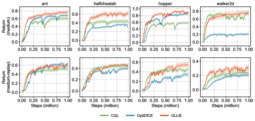
Figure 5: Comparable performance in offline RL. The results are normalized and averaged over five random seeds with standard deviation depicted by uncertainty intervals. We employ the medium and random datasets from D4RL.

Appendix F Experimental Setup

F.1 Environments and Tasks

We evaluate our method on a number of environments (Robomimic, MuJoCo, Adroit, FrankaKitchen, and AntMaze) which are widely used in prior studies (Nakamoto et al., 2023; Watson et al., 2024). We elaborate in what follows.

• Vision-based Robomimic. The Robomimic tasks (lift, can, square) involve controlling a 7-DoF simulated hand robot (Mandlekar et al., 2022), with pixelized observations as shown in Fig. 6. The robot is tasked with lifting objects, picking and placing cans, and picking up a square nut to place it on a rod from random initializations.

  

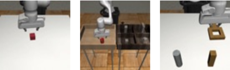
  Figure 6: Observations of vision-based Robomimic tasks. From left to right: lift, can, square.

• Vision-based MuJoCo. The MuJoCo locomotion tasks (ant, hopper, halfcheetah, walker2d) are popular benchmarks used in existing work. In addition to the standard setting, we also consider vision-based MuJoCo tasks which uses the image observation as input (see Fig. 7).

  

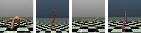
  Figure 7: Observations of vision-based MuJoCo tasks. From left to right: ant, hopper, halfcheetah, walker2d.

• Adroit. The Adroit tasks (hammer, door, pen, and relocate) (Rajeswaran et al., 2017) involve controlling a 28-DoF hand with five fingers tasked with hammering a nail, opening a door, twirling a pen, or picking up and moving a ball.

  

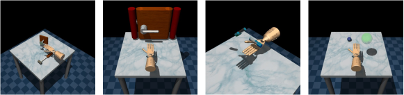
  Figure 8: Adroit tasks: hammer, door, pen, and relocate (from left to right).

• FrankaKitchen. The FrankaKitchen tasks (complete, partial, undirect), proposed by Gupta et al. (2019), involve controlling a 9-DoF Franka robot in a kitchen environment containing several common household items: a microwave, a kettle, an overhead light, cabinets, and an oven. The goal of each task is to interact with the items to reach a desired goal configuration. In the undirect task, the robot requires opening the microwave. In the partial task, the robot must first opening the microwave and subsequently moving the kettle. In the complete task, the robot need to open the microwave, move the kettle, flip the light switch, and slide open the cabinet door sequentially (see Fig. 9). These tasks are especially challenging, since they require composing parts of trajectories, preciselong-horizon manipulation, and handling human-provided teleoperation data.

  

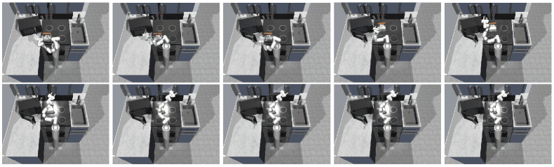
  Figure 9: Visualized success for opening the microwave, moving the kettle, turning on the light switch, sliding the slider.

• AntMaze. The AntMaze tasks require controlling an 8-Degree of Freedom (DoF) quadruped robot to move from a startingpoint to a fixed goal location (Fu et al., 2020). Three maze layouts (umaze, medium, and large) are provided from small to large.

  

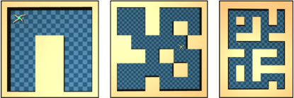
  Figure 10: AntMaze with three maze layouts, umaze, medium, and large (from left to right).

Detailed information about the environments including observation space, action space, and expert performance is provided in Tables 2 and 3, where expert and random scores are averaged over 1000 episodes.

Table 2: Details of continuous-control tasks.

Task	State dim.	Action dim.	random*	expert*
ant	$27$	$8$	$-325.60$	$3879.70$
halfcheetah	$17$	$6$	$-280.18$	$12135.00$
hopper	$11$	$3$	$-20.27$	$3234.30$
walker2d	$17$	$6$	$1.63$	$4592.30$
antmaze	$27$	$8$	$0.00$	$1.00$
door	$39$	$28$	$-56.51$	$2880.57$
hammer	$46$	$26$	$-274.86$	$12794.13$
pen	$45$	$24$	$96.26$	$3076.83$
relocate	$39$	$30$	$-6.43$	$4233.88$
FrankaKitchen	$59$	$9$	$0.00$	$1.00$

• Average scores over 1000 trajectories of expert and random.

Table 3: Details of vision-based tasks.

Task	State dim.	Action dim.	random*	expert*
ant	($84\times 84$)	$8$	$-325.60$	$3879.70$
halfcheetah	($84\times 84$)	$6$	$-280.18$	$12135.00$
hopper	($84\times 84$)	$3$	$-20.27$	$3234.30$
walker2d	($84\times 84$)	$6$	$1.63$	$4592.30$
lift	($84\times 84$)	$7$	$0.00$	$1.00$
can	($84\times 84$)	$7$	$0.00$	$1.00$
square	($84\times 84$)	$7$	$0.00$	$1.00$

• Average scores over 1000 trajectories of expert and random.

F.2 Datasets

During offline training, we use the D4RL datasets (Fu et al., 2020) for AntMaze, MuJoCo, Adroit, and FrankaKitchen, and we use the robomimic (Mandlekar et al., 2022) datasets for Robomimic. creftable:dataset details the specific datasets used for the expert and imperfect data in each task (the exploited numbers of expert and imperfect trajectories may vary across experiments). In addition, we construct vision-based MuJoCo datasets using the same method as Fu et al. (2020): the expert and imperfect data use video samples from a policy trained to completion with SAC (Haarnoja et al., 2018) and a randomly initialized policy, respectively.

Table 4: Datasets used in different tasks.

Domain	Dataset	Task	Expert data	Imperfect data
MuJoCo	D4RL	ant	ant-expert-v2	ant-random-v2
				ant-medium-replay-v2
				ant-medium-v2
				ant-medium-expert-v2
		hopper	hopper-expert-v2	hopper-random-v2
				hopper-medium-replay-v2
				hopper-medium-v2
				hopper-medium-expert-v2
		halfcheetah	halfcheetah-expert-v2	halfcheetah-random-v2
				halfcheetah-medium-replay-v2
				halfcheetah-medium-v2
				halfcheetah-medium-expert-v2
		walker2d	walker2d-expert-v2	walker2d-random-v2
				walker2d-medium-replay-v2
				walker2d-medium-v2
				walker2d-medium-expert-v2
Adroit	D4RL	pen	pen-expert-v1	pen-cloned-v1
				pen-human-v1
		hammer	hammer-expert-v1	hammer-cloned-v1
				hammer-human-v1
		door	door-expert-v1	door-cloned-v1
				door-human-v1
		relocate	relocate-expert-v1	relocate-cloned-v1
				relocate-human-v1
AntMaze	D4RL	umaze	antmaze-umaze-v0	antmaze-umaze-diverse-v0
		medium	antmaze-medium-v0	antmaze-medium-diverse-v0
		large	antmaze-large-v0	antmaze-large-diverse-v0
FrankaKitchen	D4RL	complete	kitchen-complete-v0	kitchen-mixed-v0
		partial	kitchen-partial-v0	kitchen-mixed-v0
		indirect	kitchen-partial-v0	kitchen-mixed-v0
Robomimic	robomimic	lift	lift-proficient-human	lift-paired-bad
		can-paired-bad	can-proficient-human	can-paired-bad
		square-paired-bad	square-proficient-human	square-paired-bad
MuJoCo (vision)	-	-	collected by expert policies	collected by random policies

• In the experiments on demonstration efficiency, we employ random for MuJoCo tasks and cloned for Adroit tasks.

• For vision-based MuJoCo tasks, the expert and imperfect data use video samples from a policy trained to completion with SAC (Haarnoja et al., 2018) and a randomly initialized policy, respectively.

F.3 Baselines

We test our method against four strong offline IL methods, all of which support the utilization of supplementary imperfect demonstrations (see Appendix A for details). We implement them based on their publicly available implementations with the same policy network structures as ours. The tuned codes are included in the supplementary material.

1. Discriminator-Weighted Behavioral Cloning (DWBC) (Xu et al., 2022a) that jointly trains a discriminator to carefully re-weight the BC objective (https://github.com/ryanxhr/DWBC);

2. Importance-Sampling-Weighted Behavioral Cloning (ISWBC) (Li et al., 2023b) that adopts importance sampling to enhance BC (https://github.com/liziniu/ISWBC).

3. Maximum Likelihood-Inverse Reinforcement Learning (MLIRL) (Zeng et al., 2023), a recent model-based offline IRL algorithm (https://github.com/Cloud0723/Offline-MLIRL).

4. Coherent Soft Imitation Learning (CSIL) (Watson et al., 2024), a model-free offline IRL method that learns a shaped reward function by entropy-regularized BC. The learned reward function can be exploited to anotate additional offline data and subsequently engage in offline RL, or used in finetuning the policy with further environmental interactions (https://joemwatson.github.io/csil).

We also compare our results to that of standard BC and its counterpart with union offline data (running BC on $\mathcal{D}_{o}$), termed NBCU (Li et al., 2023b). During online fintuning, we continue training the policies pretrained from the offline IL methods BC, NBCU, DWBC, ISWBC, and MLIRL by GAIL (https://github.com/Khrylx/PyTorch-RL) with the hyperparameters recommended by Orsini et al. (2021). In addition, we also compare with another instantiation of tuning MLIRL, which runs SAC with its offline learned reward function (Section G.3.5). However, we find the results not competitive and skip it out of our main results for brevity.

F.4 Implementation Details

Our method is straightforward to implement and forgiving to hyperparameters. Of note, except for the network structures in vision-based tasks (requiring the employment of CNNs), all hyperparameters are identical across tasks and settings.

For all neural nets, we adopt ReLU as activations, Adam as the optimizer, and 256 as the batchsize. For vision-based tasks, a simple CNN architecture is employed for the discriminator ($\phi_{d}$) and dual ‘variables’ ($\phi_{\nu}$ and $\phi_{y}$), comprising two convolutional layers, each with a $3\times 3$ convolutional kernel, $2\times 2$ max pooling. For the other tasks, we represent $\phi_{d}$, $\phi_{\nu}$, $\phi_{y}$ as 2-layer feedforward neural networks with $256$ hidden units. The policy networks share the same structures but generate Tanh Gaussian outputs. The output of $\phi_{d}$ is clipped to $[0.1,0.9]$ for training stability. The learning rates for the policy, $\phi_{d}$, $\phi_{\nu}$, $\phi_{y}$, $D_{\phi_{y},\phi_{v}}$ are 1e-4, 1e-5, 3e-4, 3e-4, 1e-4, respectively. The hyperparameters are summarized in Table 5.

Table 5: Hyperparameters (identical across tasks).

Hyperparameter	Value
Optimizer	Adam
Activation function	ReLU
Batchsize	256
Policy learning rate (offline/online)	1e-4
Learning rate of $\phi_{d},D_{\phi_{y},\phi_{d}}$	1e-5
Learning rate of $\phi_{v}$ and $\phi_{y}$	3e-4
Discount factor $\gamma$	0.99

We employ the forward-KL-divergence-based policy extraction in our experiments (the comparison between forward and reverse methods is included in Section G.3.7). We implement our code using Pytorch 1.8.1, built upon the open-source framework of offline RL algorithms, provided at https://github.com/tinkoff-ai/CORL (under the Apache-2.0 License) and the implementation of DWBC, provided at https://github.com/ryanxhr/DWBC (under the MIT License). All the experiments are run on Ubuntu 20.04.2 LTS with 8 NVIDIA GeForce RTX 4090 GPUs.

F.5 Performance Measure

We train a policy using 5 random seeds and evaluate it by running it in the environment for 10 episodes and computing the average undiscounted return of the environment reward. Akin to Fu et al. (2020), we use the normalized scores in figures and tables, which are measured by $\texttt{score}=\frac{\texttt{score}-\texttt{random\_score}}{\texttt{expert\_score}-\texttt{random\_score}}$ or $\texttt{score}=100\times\frac{\texttt{score}-\texttt{random\_score}}{\texttt{expert\_score}-\texttt{random\_score}}$.

Appendix G Experimental Results

This section provides full experimental results to comprehensively answer the questions raised in Section 7. We also provide some complementary experiments for a better understanding of the proposed method in Section G.3.

G.1 Performance in Offline Imitation Learning

G.1.1 Demonstration Effeciency

First, we evaluate OLLIE’s performance in offline IL with varying quantities of expert trajectories, ranging from 1 to 30 in AntMaze and MuJuCo, from 10 to 300 in Adroit and FrankaKitchen, and from 25 to 200 in vision-based MuJoCo and Robomimic. The number of imperfect trajectories is set as 1000. The sampling datasets can be found in Table 4. The comparative results and learning curves are shown below.

Summary of key findings. OLLIE consistently and significantly outperforms existing methods in terms of the performance, convergence speed, and demonstration efficiency, especially in challenging robotic manipulation and vision-based tasks.

Table 6: Normalized performance in offline IL.

(# expert trajectories: 1 in AntMaze/MuJoCo and 10 in Adroit/FrankaKitchen) Task OLLIE BC NBCU CSIL DWBC MLIRL ISWBC ant $\bm{57.1\pm 7.0}$ $-10.7\pm 11.7$ $31.1\pm 7.0$ $2.8\pm 1.3$ $24.5\pm 1.1$ $39.3\pm 9.0$ $30.4\pm 7.7$ halfcheetah $\bm{35.5\pm 4.0}$ $0.2\pm 1.0$ $2.2\pm 0.1$ $22.9\pm 2.8$ $0.0\pm 0.0$ $23.8\pm 1.0$ $13.7\pm 3.0$ hopper $71.1\pm 3.5$ $17.8\pm 5.4$ $6.6\pm 3.9$ $17.1\pm 6.8$ $\bm{77.8\pm 12.7}$ $54.7\pm 16.7$ $64.7\pm 9.9$ walker2d $\bm{59.8\pm 8.5}$ $4.6\pm 3.9$ $0.0\pm 0.0$ $8.1\pm 5.6$ $56.9\pm 11.6$ $49.9\pm 6.7$ $48.2\pm 4.7$ umaze $\bm{75.4\pm 3.8}$ $3.5\pm 3.4$ $4.5\pm 4.3$ $11.1\pm 4.9$ $23.1\pm 3.9$ $7.8\pm 3.9$ $10.1\pm 1.3$ medium $\bm{58.4\pm 7.3}$ $0.0\pm 0.0$ $0.0\pm 0.0$ $1.0\pm 1.0$ $0.0\pm 0.0$ $0.0\pm 0.0$ $7.2\pm 6.7$ large $\bm{37.5\pm 4.3}$ $0.0\pm 0.0$ $0.0\pm 0.0$ $1.0\pm 1.0$ $0.0\pm 0.0$ $0.0\pm 0.0$ $5.3\pm 1.9$ hammer $\bm{46.1\pm 6.5}$ $5.7\pm 6.8$ $0.0\pm 0.0$ $16.7\pm 8.9$ $6.6\pm 8.3$ $1.0\pm 0.1$ $6.5\pm 5.1$ pen $\bm{67.4\pm 5.6}$ $40.3\pm 10.3$ $3.2\pm 9.8$ $39.0\pm 5.6$ $42.8\pm 19.3$ $18.7\pm 2.6$ $49.5\pm 2.9$ door $\bm{28.9\pm 2.9}$ $2.8\pm 3.9$ $0.0\pm 0.0$ $24.8\pm 3.6$ $0.0\pm 0.0$ $1.0\pm 0.8$ $2.9\pm 2.1$ relocate $\bm{31.2\pm 5.8}$ $0.0\pm 0.0$ $0.0\pm 0.0$ $7.7\pm 8.8$ $0.0\pm 0.0$ $1.0\pm 0.2$ $0.0\pm 0.0$ paritial $\bm{34.6\pm 6.6}$ $1.0\pm 0.5$ $0.0\pm 0.0$ $26.1\pm 1.4$ $1.0\pm 1.4$ $1.0\pm 0.7$ $3.4\pm 1.1$ complete $\bm{34.9\pm 1.8}$ $1.0\pm 0.3$ $0.0\pm 0.0$ $19.1\pm 7.9$ $1.0\pm 0.6$ $1.0\pm 0.8$ $3.1\pm 1.9$ undirect $\bm{48.1\pm 3.9}$ $1.0\pm 0.2$ $0.0\pm 0.0$ $37.0\pm 9.0$ $-1.0\pm 1.6$ $1.0\pm 0.8$ $3.1\pm 1.0$

Table 7: Normalized performance in offline IL.

(# expert trajectories: 3 in AntMaze/MuJoCo and 30 in Adroit/FrankaKitchen) Task OLLIE BC NBCU CSIL DWBC MLIRL ISWBC ant $\bm{78.0\pm 6.2}$ $50.5\pm 27.8$ $28.9\pm 3.4$ $10.4\pm 1.2$ $32.3\pm 10.1$ $51.2\pm 7.2$ $30.2\pm 2.3$ halfcheetah $\bm{79.5\pm 6.1}$ $5.7\pm 1.1$ $3.7\pm 1.3$ $20.0\pm 3.8$ $50.9\pm 11.1$ $66.6\pm 3.4$ $37.4\pm 7.1$ hopper $\bm{88.7\pm 6.9}$ $47.3\pm 6.7$ $10.6\pm 3.2$ $73.9\pm 3.9$ $79.8\pm 14.0$ $74.8\pm 13.6$ $53.8\pm 3.9$ walker2d $75.6\pm 2.8$ $14.8\pm 2.1$ $5.6\pm 1.9$ $17.3\pm 5.4$ $62.6\pm 3.2$ $\bm{87.2\pm 11.7}$ $60.9\pm 2.2$ umaze $\bm{90.6\pm 3.1}$ $22.4\pm 9.6$ $30.4\pm 12.9$ $55.1\pm 5.5$ $51.8\pm 3.0$ $37.2\pm 6.6$ $28.6\pm 2.5$ medium $\bm{72.8\pm 6.2}$ $0.0\pm 0.0$ $0.0\pm 0.0$ $32.5\pm 4.5$ $4.6\pm 1.7$ $23.5\pm 6.9$ $15.3\pm 5.7$ large $\bm{48.5\pm 1.4}$ $0.0\pm 0.0$ $0.0\pm 0.0$ $19.3\pm 1.5$ $0.0\pm 0.0$ $12.3\pm 3.2$ $10.2\pm 7.3$ hammer $\bm{69.5\pm 8.5}$ $1.0\pm 1.0$ $1.0\pm 1.0$ $51.1\pm 9.4$ $1.0\pm 0.0$ $1.0\pm 0.0$ $9.1\pm 4.3$ pen $\bm{76.3\pm 3.6}$ $54.2\pm 15.4$ $27.1\pm 6.8$ $47.9\pm 12.0$ $55.6\pm 13.7$ $57.1\pm 9.1$ $64.3\pm 8.1$ door $\bm{66.3\pm 3.7}$ $3.7\pm 1.9$ $2.9\pm 1.3$ $48.4\pm 3.9$ $2.4\pm 0.3$ $1.0\pm 0.0$ $12.8\pm 2.5$ relocate $\bm{46.6\pm 6.5}$ $0.0\pm 1.0$ $0.0\pm 1.0$ $26.1\pm 6.2$ $0.0\pm 0.0$ $1.0\pm 0.0$ $8.6\pm 4.0$ paritial $\bm{69.3\pm 1.8}$ $2.7\pm 1.6$ $1.0\pm 0.0$ $61.2\pm 1.9$ $3.0\pm 1.7$ $1.0\pm 0.0$ $3.8\pm 1.9$ complete $\bm{60.9\pm 1.8}$ $2.0\pm 1.3$ $1.0\pm 0.0$ $45.9\pm 2.5$ $3.5\pm 1.7$ $10.0\pm 0.0$ $3.5\pm 1.4$ undirect $\bm{75.1\pm 1.7}$ $2.2\pm 1.8$ $1.0\pm 0.0$ $62.4\pm 8.5$ $3.1\pm 1.9$ $1.0\pm 0.0$ $5.1\pm 1.4$

Table 8: Normalized performance in offline IL.

(# expert trajectories: 5 in AntMaze/MuJoCo and 50 in Adroit/FrankaKitchen) Task OLLIE BC NBCU CSIL DWBC MLIRL ISWBC ant $\bm{105.2\pm 4.3}$ $61.9\pm 3.2$ $58.8\pm 2.5$ $61.5\pm 4.0$ $80.3\pm 2.8$ $57.3\pm 4.1$ $5.2\pm 6.8$ halfcheetah $\bm{82.0\pm 9.2}$ $31.6\pm 8.3$ $34.6\pm 6.5$ $6.2\pm 2.0$ $48.2\pm 5.6$ $83.5\pm 1.1$ $53.5\pm 2.7$ hopper $\bm{97.4\pm 4.9}$ $39.5\pm 5.7$ $25.7\pm 7.9$ $88.3\pm 5.4$ $75.8\pm 7.6$ $79.7\pm 8.5$ $64.1\pm 3.3$ walker2d $\bm{94.6\pm 2.5}$ $16.9\pm 3.6$ $17.9\pm 7.5$ $69.5\pm 6.1$ $67.1\pm 7.7$ $88.7\pm 4.9$ $61.6\pm 3.4$ umaze $\bm{100.0\pm 0.0}$ $29.6\pm 5.5$ $33.8\pm 7.0$ $82.3\pm 5.4$ $56.2\pm 5.1$ $42.4\pm 3.1$ $38.9\pm 5.8$ medium $\bm{95.0\pm 5.0}$ $1.0\pm 1.0$ $1.0\pm 1.0$ $52.1\pm 4.2$ $13.3\pm 3.7$ $28.8\pm 5.0$ $28.0\pm 4.2$ large $\bm{80.7\pm 7.8}$ $1.0\pm 1.0$ $1.0\pm 1.0$ $38.4\pm 4.9$ $7.7\pm 6.9$ $15.3\pm 5.7$ $16.9\pm 3.6$ hammer $\bm{79.3\pm 9.5}$ $1.0\pm 1.0$ $1.0\pm 1.0$ $61.4\pm 3.8$ $1.0\pm 1.0$ $1.0\pm 1.0$ $23.2\pm 5.9$ pen $\bm{86.6\pm 2.9}$ $50.5\pm 7.5$ $26.0\pm 2.5$ $63.0\pm 5.8$ $80.8\pm 5.0$ $57.4\pm 4.8$ $63.8\pm 3.5$ door $\bm{79.4\pm 4.9}$ $1.0\pm 1.0$ $1.0\pm 1.0$ $56.3\pm 7.2$ $1.0\pm 1.0$ $1.0\pm 1.0$ $23.2\pm 2.5$ relocate $\bm{69.4\pm 6.7}$ $10.0\pm 1.0$ $1.0\pm 1.0$ $6.7\pm 7.7$ $1.0\pm 1.0$ $1.0\pm 1.0$ $29.7\pm 4.3$ paritial $\bm{76.3\pm 3.7}$ $4.1\pm 6.4$ $1.0\pm 1.0$ $74.3\pm 7.9$ $1.3\pm 79.0$ $1.0\pm 1.0$ $1.0\pm 3.3$ complete $\bm{64.2\pm 4.1}$ $3.3\pm 5.2$ $1.0\pm 1.0$ $51.4\pm 5.9$ $9.4\pm 4.6$ $1.0\pm 1.0$ $4.1\pm 6.1$ undirect $\bm{74.3\pm 3.4}$ $8.6\pm 3.3$ $1.0\pm 1.0$ $84.2\pm 7.3$ $12.5\pm 4.8$ $1.0\pm 1.0$ $16.6\pm 6.1$

Table 9: Normalized performance in offline IL.

(# expert trajectories: 10 in AntMaze/MuJoCo and 100 in Adroit/FrankaKitchen) Task OLLIE BC NBCU CSIL DWBC MLIRL ISWBC ant $\bm{115.7\pm 4.3}$ $64.6\pm 6.0$ $58.9\pm 16.7$ $83.1\pm 6.1$ $88.7\pm 5.5$ $65.7\pm 4.1$ $79.4\pm 7.5$ halfcheetah $\bm{90.2\pm 10.3}$ $61.5\pm 4.0$ $3.5\pm 1.9$ $77.8\pm 7.4$ $58.9\pm 3.6$ $82.9\pm 3.9$ $77.1\pm 3.0$ hopper $\bm{99.2\pm 3.9}$ $61.8\pm 19.6$ $25.7\pm 2.6$ $95.4\pm 3.4$ $69.1\pm 3.1$ $89.2\pm 6.2$ $81.6\pm 8.4$ walker2d $\bm{95.9\pm 3.8}$ $17.6\pm 2.4$ $17.6\pm 3.4$ $91.4\pm 9.0$ $71.3\pm 9.8$ $92.0\pm 7.0$ $62.0\pm 9.0$ umaze $\bm{100.0\pm 0.0}$ $46.1\pm 3.9$ $40.4\pm 9.9$ $94.1\pm 6.2$ $69.9\pm 3.2$ $55.1\pm 13.7$ $54.3\pm 6.3$ medium $\bm{95.0\pm 5.0}$ $0.0\pm 0.0$ $0.0\pm 0.0$ $60.9\pm 3.3$ $33.4\pm 7.6$ $41.2\pm 7.3$ $48.3\pm 9.3$ large $\bm{85.0\pm 10.0}$ $0.0\pm 0.0$ $0.0\pm 0.0$ $46.2\pm 6.8$ $25.5\pm 5.6$ $21.4\pm 2.8$ $25.2\pm 4.1$ hammer $\bm{82.6\pm 9.8}$ $41.9\pm 1.5$ $1.0\pm 1.0$ $66.8\pm 5.3$ $70.6\pm 3.9$ $1.0\pm 0.0$ $43.2\pm 7.6$ pen $\bm{94.6\pm 6.6}$ $56.5\pm 7.6$ $24.0\pm 1.0$ $70.0\pm 11.8$ $69.7\pm 2.3$ $58.6\pm 5.1$ $62.6\pm 5.0$ door $\bm{92.0\pm 1.8}$ $26.6\pm 6.2$ $0.0\pm 1.0$ $59.7\pm 7.7$ $20.5\pm 6.0$ $1.0\pm 0.0$ $39.6\pm 3.3$ relocate $\bm{92.1\pm 8.5}$ $35.0\pm 4.2$ $0.0\pm 1.0$ $74.6\pm 4.3$ $38.6\pm 9.8$ $1.0\pm 0.0$ $41.2\pm 7.2$ paritial $\bm{99.1\pm 1.8}$ $10.4\pm 0.1$ $3.4\pm 1.0$ $79.0\pm 5.7$ $27.3\pm 5.7$ $1.0\pm 0.0$ $20.0\pm 2.2$ complete $\bm{98.6\pm 2.8}$ $6.1\pm 7.5$ $3.1\pm 1.0$ $54.9\pm 5.8$ $23.6\pm 1.0$ $1.0\pm 0.0$ $5.9\pm 5.7$ undirect $\bm{100.0\pm 0.0}$ $22.7\pm 5.3$ $3.5\pm 1.4$ $93.6\pm 7.4$ $34.9\pm 7.5$ $1.0\pm 0.0$ $32.6\pm 8.7$

Table 10: Normalized performance in offline IL.

(# expert trajectories: 30 in AntMaze/MuJoCo and 300 in Adroit/FrankaKitchen) Task OLLIE BC NBCU CSIL DWBC MLIRL ISWBC ant $\bm{117.5\pm 3.6}$ $100.6\pm 1.1$ $100.7\pm 2.8$ $106.8\pm 0.9$ $91.3\pm 5.4$ $107.1\pm 5.6$ $105.6\pm 8.6$ halfcheetah $\bm{100.6\pm 0.8}$ $86.4\pm 3.3$ $3.2\pm 1.9$ $102.1\pm 2.5$ $89.4\pm 4.2$ $93.6\pm 5.8$ $101.3\pm 3.3$ hopper $\bm{108.7\pm 1.2}$ $56.8\pm 17.9$ $31.9\pm 10.4$ $94.0\pm 3.7$ $107.7\pm 2.2$ $103.9\pm 7.2$ $99.1\pm 2.6$ walker2d $\bm{105.7\pm 2.9}$ $41.1\pm 21.3$ $26.5\pm 11.6$ $101.5\pm 1.4$ $97.8\pm 3.6$ $92.9\pm 13.4$ $92.0\pm 3.4$ umaze $\bm{100.0\pm 0.0}$ $65.0\pm 30.2$ $55.5\pm 25.2$ ${100.0\pm 0.0}$ $90.0\pm 5.0$ ${100.0\pm 0.0}$ ${100.0\pm 0.0}$ medium $\bm{100.0\pm 0.0}$ $0.0\pm 0.0$ $0.0\pm 0.0$ $99.0\pm 1.0$ $47.0\pm 3.0$ $71.5\pm 4.2$ $91.0\pm 3.0$ large ${100.0\pm 0.0}$ $0.0\pm 0.0$ $0.0\pm 0.0$ $79.9\pm 6.6$ $40.3\pm 3.2$ $65.1\pm 3.2$ $73.0\pm 4.0$ hammer ${100.7\pm 9.3}$ $\bm{105.8\pm 5.1}$ $0.0\pm 1.0$ $100.0\pm 3.1$ $93.8\pm 4.6$ $53.1\pm 5.9$ ${102.4\pm 2.8}$ pen $\bm{99.3\pm 3.7}$ $85.9\pm 9.3$ $57.0\pm 4.8$ $94.0\pm 6.5$ $98.9\pm 2.0$ $77.5\pm 9.6$ $92.2\pm 2.7$ door $\bm{108.5\pm 1.3}$ $34.0\pm 5.6$ $0.0\pm 1.0$ $105.7\pm 4.3$ $71.3\pm 9.4$ $41.5\pm 7.2$ $65.2\pm 4.5$ relocate ${102.7\pm 5.3}$ $101.7\pm 2.2$ $0.0\pm 1.0$ $98.6\pm 8.5$ $100.9\pm 0.1$ $82.6\pm 3.8$ $\bm{104.8\pm 5.9}$ paritial $\bm{100.0\pm 0.0}$ $34.7\pm 2.3$ $13.4\pm 2.3$ $\bm{100.0\pm 0.0}$ $58.1\pm 5.3$ $1.0\pm 0.0$ $39.9\pm 4.7$ complete $\bm{100.0\pm 0.0}$ $21.6\pm 3.8$ $10.7\pm 1.3$ $85.0\pm 7.9$ $32.3\pm 3.9$ $1.0\pm 0.0$ $28.8\pm 6.0$ undirect $\bm{100.0\pm 0.0}$ $48.7\pm 4.0$ $16.0\pm 3.7$ ${100.0\pm 0.0}$ $63.7\pm 1.0$ $1.0\pm 0.0$ $58.1\pm 3.3$

Table 11: Normalized performance in offline IL across vision-based tasks.

(# expert trajectories: 25) Task OLLIE BC NBCU CSIL DWBC MLIRL ISWBC ant $\bm{30.8\pm 5.1}$ $16.1\pm 5.5$ $16.3\pm 3.7$ $11.6\pm 3.6$ $18.2\pm 4.3$ $0.1\pm 1.0$ $22.4\pm 3.1$ halfcheetah $\bm{41.9\pm 3.1}$ $27.3\pm 4.7$ $29.5\pm 6.8$ $26.3\pm 5.8$ $19.7\pm 8.2$ $0.1\pm 1.0$ $26.0\pm 2.9$ hopper $\bm{57.2\pm 2.3}$ $13.3\pm 5.9$ $12.8\pm 7.2$ $12.7\pm 5.3$ $17.6\pm 3.9$ $0.1\pm 1.0$ $16.1\pm 8.4$ walker2d $\bm{53.3\pm 2.6}$ $10.3\pm 3.2$ $8.0\pm 8.0$ $9.0\pm 8.2$ $26.5\pm 7.7$ $0.1\pm 1.0$ $28.4\pm 4.7$ lift $\bm{84.6\pm 6.9}$ $49.0\pm 6.6$ $29.9\pm 4.2$ $53.7\pm 3.4$ $47.7\pm 7.8$ $0.1\pm 1.0$ $57.1\pm 3.1$ can $\bm{39.8\pm 7.8}$ $14.1\pm 12.2$ $22.3\pm 3.9$ $24.4\pm 4.8$ $25.0\pm 2.1$ $0.1\pm 1.0$ $10.7\pm 15.8$ square $\bm{36.1\pm 8.0}$ $2.1\pm 2.1$ $5.5\pm 5.0$ $5.2\pm 4.3$ $17.1\pm 4.5$ $0.1\pm 1.0$ $15.3\pm 2.3$

Table 12: Normalized performance in offline IL across vision-based tasks.

(# expert trajectories: 50) Task OLLIE BC NBCU CSIL DWBC MLIRL ISWBC ant $\bm{58.6\pm 7.2}$ $26.8\pm 9.7$ $25.4\pm 3.9$ $20.5\pm 6.8$ $28.6\pm 3.5$ $0.0\pm 1.0$ $32.7\pm 4.4$ halfcheetah $\bm{61.7\pm 6.7}$ $42.7\pm 7.2$ $23.8\pm 4.7$ $19.7\pm 5.2$ $26.6\pm 6.6$ $0.0\pm 1.0$ $35.3\pm 5.8$ hopper $\bm{85.2\pm 6.4}$ $21.3\pm 8.4$ $13.7\pm 9.3$ $18.8\pm 5.7$ $16.9\pm 3.2$ $0.0\pm 1.0$ $23.5\pm 4.7$ walker2d $\bm{64.5\pm 8.6}$ $22.0\pm 6.5$ $15.5\pm 5.5$ $24.6\pm 9.4$ $27.6\pm 5.0$ $0.0\pm 1.0$ $38.3\pm 5.5$ lift $\bm{95.0\pm 5.0}$ $75.6\pm 8.2$ $63.3\pm 7.0$ $62.4\pm 2.8$ $70.1\pm 8.8$ $0.0\pm 0.0$ $77.2\pm 5.3$ can $\bm{61.3\pm 5.3}$ $25.0\pm 11.2$ $23.9\pm 4.5$ $38.9\pm 2.5$ $28.6\pm 9.5$ $0.0\pm 0.0$ $32.8\pm 3.8$ square $\bm{41.3\pm 8.3}$ $17.0\pm 7.4$ $15.9\pm 4.9$ $17.4\pm 3.2$ $18.3\pm 5.3$ $0.0\pm 0.0$ $24.5\pm 5.1$

Table 13: Normalized performance in offline IL across vision-based tasks.

(# expert trajectories: 100) Task OLLIE BC NBCU CSIL DWBC MLIRL ISWBC ant $\bm{71.1\pm 3.9}$ $43.7\pm 2.7$ $38.0\pm 6.0$ $43.9\pm 4.6$ $26.0\pm 3.8$ $0.0\pm 1.0$ $45.4\pm 9.6$ halfcheetah $\bm{75.8\pm 4.3}$ $50.9\pm 5.4$ $38.0\pm 2.7$ $44.0\pm 5.5$ $18.2\pm 2.7$ $0.0\pm 1.0$ $55.3\pm 4.6$ hopper $\bm{91.7\pm 2.7}$ $31.2\pm 2.6$ $30.8\pm 6.8$ $29.4\pm 7.9$ $23.6\pm 9.0$ $0.0\pm 1.0$ $33.6\pm 2.1$ walker2d $\bm{82.1\pm 8.1}$ $39.4\pm 6.9$ $40.2\pm 5.0$ $49.1\pm 7.2$ $35.9\pm 2.7$ $0.0\pm 1.0$ $48.2\pm 5.4$ lift $\bm{99.0\pm 1.0}$ $89.0\pm 11.0$ $91.0\pm 9.0$ $62.9\pm 2.5$ $94.0\pm 6.0$ $0.0\pm 0.0$ $95.0\pm 5.0$ can $\bm{78.0\pm 7.5}$ $49.7\pm 5.2$ $58.8\pm 8.7$ $51.6\pm 1.4$ $56.2\pm 3.9$ $0.0\pm 0.0$ $55.8\pm 2.9$ square $\bm{64.1\pm 6.4}$ $31.9\pm 6.9$ $24.3\pm 4.7$ $24.9\pm 3.6$ $22.6\pm 5.3$ $0.0\pm 0.0$ $27.8\pm 8.6$

Table 14: Normalized performance in offline IL across vision-based tasks.

(# expert trajectories: 200) Task OLLIE BC NBCU CSIL DWBC MLIRL ISWBC ant $\bm{82.0\pm 4.5}$ $48.5\pm 5.3$ $57.0\pm 5.1$ $57.8\pm 3.3$ $15.0\pm 4.2$ $0.0\pm 1.0$ $59.6\pm 4.2$ halfcheetah $\bm{93.9\pm 7.8}$ $54.6\pm 6.1$ $58.7\pm 6.0$ $59.1\pm 5.5$ $34.6\pm 7.1$ $0.0\pm 1.0$ $60.7\pm 4.8$ hopper $\bm{98.0\pm 3.3}$ $56.6\pm 2.4$ $49.1\pm 9.1$ $45.0\pm 2.9$ $12.5\pm 7.2$ $0.0\pm 1.0$ $47.7\pm 2.8$ walker2d $\bm{90.3\pm 5.9}$ $43.5\pm 5.4$ $73.1\pm 6.1$ $71.0\pm 4.4$ $10.1\pm 8.4$ $0.0\pm 1.0$ $71.4\pm 6.3$ lift $\bm{100.0\pm 0.0}$ $91.0\pm 9.0$ $97.0\pm 3.0$ $63.1\pm 2.0$ $95.0\pm 5.0$ $0.0\pm 0.0$ $94.0\pm 6.0$ can $\bm{94.0\pm 6.0}$ $66.8\pm 11.1$ $64.8\pm 4.8$ $57.6\pm 3.4$ $73.6\pm 4.2$ $0.0\pm 0.0$ $83.9\pm 5.0$ square $\bm{85.2\pm 4.4}$ $37.5\pm 12.7$ $33.7\pm 6.9$ $35.5\pm 3.1$ $16.5\pm 1.6$ $0.0\pm 0.0$ $34.9\pm 4.4$

Figure 12: Learning curves in offline IL with varying quantities of expert trajectories in MuJoCo. Uncertainty intervals depict standard deviation over five seeds. $n_{e}$ represents expert trajectories. OLLIE consistently exhibits fast and stabilized convergence.

Figure 13: Performance in offline IL with varying quantities of expert trajectories in Adroit. Uncertainty intervals depict standard deviation over five seeds. OLLIE uses fewer expert demonstrations to attain expert performance, demonstrating its great demonstration efficiency in comparison with existing methods.

Figure 14: Learning curves in offline IL with varying quantities of expert trajectories in Adroit. Uncertainty intervals depict standard deviation over five seeds. $n_{e}$ represents expert trajectories. OLLIE consistently exhibits fast and stabilized convergence.

Figure 15: Performance in offline IL with varying quantities of expert trajectories in AntMaze. Uncertainty intervals depict standard deviation over five seeds. $n_{e}$ represents expert trajectories. OLLIE uses much fewer expert demonstrations to attain expert performance, demonstrating its great demonstration efficiency in comparison with existing methods. Of note, AntMaze is challenging because it requires precise long-horizon control. The outperformance of OLLIE reveals its capability of extracting environmental information from offline data.

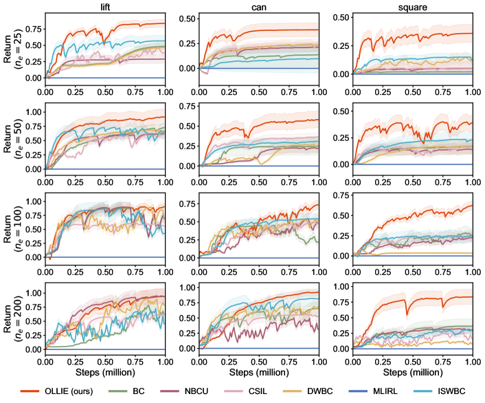
Figure 22: Learning curves in offline IL with varying quantities of expert trajectories in vision-based Robomimic. Uncertainty intervals depict standard deviation over five seeds. $n_{e}$ represents expert trajectories. OLLIE consistently exhibits fast and stabilized convergence.

G.1.2 Data Quality

Then, we conduct experiments using imperfect demonstrations with varying qualities to test the robustness of ILID’s performance. We present the result and data setup in Table 1. OLLIE outperforms the baselines in 20 out of 24 settings. The corresponding learning curves of Table 1 are depicted in Figs. 23 and 24.

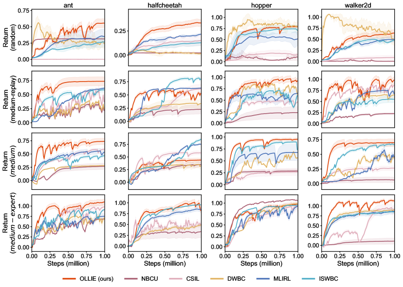
Figure 23: Learning curves in offline IL with varying qualities of imperfect trajectories in MuJoCo. Uncertainty intervals depict standard deviation over five seeds. We use 1 expert trajectory, sampled from expert of D4RL, and 1000 imperfect trajectories, sampled from the corresponding datasets listed in Table 1. The length of each trajectory is less than 1000 time steps. OLLIE consistently exhibits fast and stabilized convergence. A higher quality of imperfect demonstrations often speeds up the convergence.

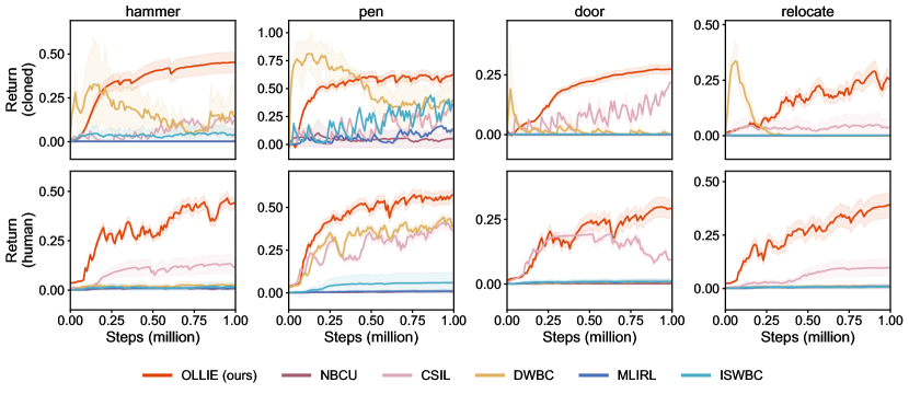
Figure 24: Learning curves in offline IL with varying qualities of imperfect trajectories in Adroid. Uncertainty intervals depict standard deviation over five seeds. We use 10 expert trajectories, sampled from expert of D4RL, and 1000 imperfect trajectories, sampled from the corresponding datasets listed in Table 1. The length of each trajectory is less than 100 time steps. In contrast with the results in relatively low-dimensional MuJoCo, OLLIE significantly outperforms the baselines in this domain, demonstrating its robustness in complex and high-dimensional environments.

G.2 Performance in Online Finetuning

After obtaining pretraining policies, we examine the finetuning performance under different quantities of expert demonstrations. In Tables 15, 16, 17, 18, 19, 20, 21, 22 and 23, we provide the performance before and after online finetuning with 10 episodes; subsequently, we present the end-to-end learning curves from offline pretraining to online finetuning across all tasks.

Summary of key findings. OLLIE successfully overcomes the unlearning problem and enables fast online finetuning that enables substantial performance improvement within a limited number of episodes. Importantly, OLLIE can work well in the cases where GAIL fails (as illustrated in Figs. 30 and 36), highlighting the importance of pretraining IL.

Table 15: Normalized performance before and after online finetuning with 10 episodes.

(# expert trajectories: 1 in AntMaze/MuJoCo and 10 in Adroit/FrankaKitchen) Task OLLIE BC NBCU CSIL DWBC MLIRL ISWBC ant $55\rightarrow\bm{83}$ $31\rightarrow 00$ $00\rightarrow 36$ $00\rightarrow 42$ $23\rightarrow 13$ $34\rightarrow 24$ $26\rightarrow 16$ halfcheetah $33\rightarrow\bm{47}$ $02\rightarrow 02$ $00\rightarrow 12$ $15\rightarrow 40$ $00\rightarrow 02$ $22\rightarrow 14$ $12\rightarrow 07$ hopper $80\rightarrow\bm{90}$ $07\rightarrow 21$ $00\rightarrow 14$ $16\rightarrow 69$ $76\rightarrow 44$ $52\rightarrow 32$ $67\rightarrow 39$ walker2d $64\rightarrow\bm{64}$ $00\rightarrow 02$ $00\rightarrow 10$ $08\rightarrow 20$ $57\rightarrow 31$ $50\rightarrow 29$ $47\rightarrow 35$ hammer $45\rightarrow\bm{53}$ $00\rightarrow 00$ $00\rightarrow 00$ $15\rightarrow 24$ $08\rightarrow 02$ $00\rightarrow 00$ $04\rightarrow 02$ pen $64\rightarrow\bm{72}$ $05\rightarrow 35$ $00\rightarrow 06$ $34\rightarrow 41$ $38\rightarrow 23$ $17\rightarrow 09$ $47\rightarrow 25$ door $27\rightarrow\bm{48}$ $00\rightarrow 02$ $00\rightarrow 00$ $05\rightarrow 92$ $00\rightarrow 01$ $00\rightarrow 01$ $00\rightarrow 01$ relocate $24\rightarrow\bm{38}$ $00\rightarrow 03$ $00\rightarrow 07$ $04\rightarrow 09$ $00\rightarrow 03$ $00\rightarrow 02$ $00\rightarrow 00$ umaze $75\rightarrow\bm{85}$ $03\rightarrow 02$ $00\rightarrow 00$ $12\rightarrow 22$ $22\rightarrow 14$ $06\rightarrow 04$ $09\rightarrow 06$ medium $56\rightarrow\bm{67}$ $00\rightarrow 00$ $00\rightarrow 00$ $00\rightarrow 15$ $00\rightarrow 00$ $00\rightarrow 00$ $06\rightarrow 04$ large $35\rightarrow\bm{61}$ $00\rightarrow 00$ $00\rightarrow 00$ $00\rightarrow 06$ $00\rightarrow 00$ $00\rightarrow 00$ $04\rightarrow 03$ complete $33\rightarrow\bm{43}$ $00\rightarrow 03$ $00\rightarrow 02$ $16\rightarrow 15$ $00\rightarrow 00$ $00\rightarrow 00$ $00\rightarrow 02$ partial $32\rightarrow\bm{44}$ $00\rightarrow 01$ $00\rightarrow 07$ $25\rightarrow 27$ $00\rightarrow 00$ $00\rightarrow 00$ $00\rightarrow 02$ undirect $36\rightarrow\bm{58}$ $00\rightarrow 11$ $00\rightarrow 23$ $36\rightarrow 35$ $00\rightarrow 00$ $00\rightarrow 00$ $00\rightarrow 01$

Table 16: Normalized performance before and after online finetuning with 10 episodes.

(# expert trajectories: 3 in AntMaze/MuJoCo and 30 in Adroit/FrankaKitchen) Task OLLIE BC NBCU CSIL DWBC MLIRL ISWBC ant $75\rightarrow\bm{82}$ $27\rightarrow 47$ $00\rightarrow 19$ $08\rightarrow 42$ $30\rightarrow 23$ $49\rightarrow 31$ $29\rightarrow 18$ halfcheetah $75\rightarrow\bm{84}$ $02\rightarrow 17$ $00\rightarrow 26$ $21\rightarrow 58$ $45\rightarrow 32$ $56\rightarrow 45$ $28\rightarrow 29$ hopper $85\rightarrow\bm{91}$ $10\rightarrow 53$ $00\rightarrow 06$ $64\rightarrow 82$ $70\rightarrow 54$ $66\rightarrow 53$ $38\rightarrow 43$ walker2d $74\rightarrow\bm{89}$ $03\rightarrow 21$ $00\rightarrow 63$ $18\rightarrow 67$ $70\rightarrow 52$ $83\rightarrow 36$ $53\rightarrow 35$ hammer $44\rightarrow\bm{85}$ $00\rightarrow 00$ $00\rightarrow 00$ $22\rightarrow 46$ $01\rightarrow 00$ $00\rightarrow 00$ $10\rightarrow 06$ pen $71\rightarrow\bm{89}$ $15\rightarrow 54$ $00\rightarrow 11$ $47\rightarrow 50$ $48\rightarrow 60$ $39\rightarrow 38$ $36\rightarrow 46$ door $61\rightarrow\bm{89}$ $03\rightarrow 44$ $00\rightarrow 00$ $45\rightarrow 46$ $00\rightarrow 01$ $00\rightarrow 00$ $05\rightarrow 08$ relocate $44\rightarrow\bm{52}$ $00\rightarrow 12$ $00\rightarrow 06$ $26\rightarrow 26$ $00\rightarrow 00$ $00\rightarrow 00$ $09\rightarrow 05$ umaze $85\rightarrow\bm{95}$ $29\rightarrow 28$ $00\rightarrow 04$ $50\rightarrow 69$ $28\rightarrow 42$ $32\rightarrow 23$ $02\rightarrow 21$ medium $70\rightarrow\bm{81}$ $00\rightarrow 00$ $00\rightarrow 00$ $12\rightarrow 51$ $03\rightarrow 03$ $22\rightarrow 17$ $15\rightarrow 13$ large $47\rightarrow\bm{73}$ $00\rightarrow 00$ $00\rightarrow 00$ $18\rightarrow 20$ $00\rightarrow 00$ $11\rightarrow 09$ $09\rightarrow 04$ complete $60\rightarrow\bm{61}$ $00\rightarrow 28$ $00\rightarrow 07$ $04\rightarrow 44$ $00\rightarrow 02$ $00\rightarrow 00$ $00\rightarrow 02$ partial $66\rightarrow\bm{72}$ $00\rightarrow 36$ $00\rightarrow 20$ $24\rightarrow 50$ $00\rightarrow 02$ $00\rightarrow 00$ $00\rightarrow 02$ undirect $73\rightarrow\bm{84}$ $00\rightarrow 18$ $00\rightarrow 07$ $62\rightarrow 48$ $00\rightarrow 01$ $00\rightarrow 00$ $05\rightarrow 03$

Table 17: Normalized performance before and after online finetuning with 10 episodes.

(# expert trajectories: 5 in AntMaze/MuJoCo and 50 in Adroit/FrankaKitchen) Task OLLIE BC NBCU CSIL DWBC MLIRL ISWBC ant $103\rightarrow\bm{112}$ $55\rightarrow 40$ $00\rightarrow 13$ $59\rightarrow 65$ $78\rightarrow 53$ $56\rightarrow 40$ $49\rightarrow 31$ halfcheetah $075\rightarrow\bm{097}$ $33\rightarrow 19$ $00\rightarrow 41$ $59\rightarrow 61$ $47\rightarrow 29$ $80\rightarrow 61$ $51\rightarrow 34$ hopper $061\rightarrow\bm{099}$ $19\rightarrow 27$ $00\rightarrow 21$ $85\rightarrow 87$ $74\rightarrow 46$ $76\rightarrow 52$ $63\rightarrow 41$ walker2d $092\rightarrow\bm{109}$ $12\rightarrow 11$ $00\rightarrow 54$ $68\rightarrow 71$ $66\rightarrow 43$ $87\rightarrow 56$ $60\rightarrow 44$ hammer $075\rightarrow\bm{093}$ $00\rightarrow 00$ $00\rightarrow 00$ $60\rightarrow 58$ $00\rightarrow 00$ $00\rightarrow 00$ $22\rightarrow 15$ pen $085\rightarrow\bm{094}$ $25\rightarrow 35$ $00\rightarrow 12$ $62\rightarrow 63$ $79\rightarrow 75$ $56\rightarrow 41$ $61\rightarrow 41$ door $076\rightarrow\bm{096}$ $00\rightarrow 00$ $00\rightarrow 03$ $55\rightarrow 54$ $00\rightarrow 00$ $00\rightarrow 00$ $21\rightarrow 15$ relocate $068\rightarrow\bm{084}$ $00\rightarrow 00$ $00\rightarrow 33$ $59\rightarrow 60$ $00\rightarrow 00$ $00\rightarrow 00$ $28\rightarrow 19$ umaze $098\rightarrow\bm{099}$ $32\rightarrow 20$ $00\rightarrow 10$ $81\rightarrow 78$ $54\rightarrow 36$ $39\rightarrow 31$ $35\rightarrow 24$ medium $093\rightarrow\bm{096}$ $00\rightarrow 00$ $00\rightarrow 00$ $51\rightarrow 44$ $12\rightarrow 09$ $27\rightarrow 18$ $26\rightarrow 20$ large $079\rightarrow\bm{088}$ $00\rightarrow 00$ $00\rightarrow 00$ $37\rightarrow 26$ $06\rightarrow 04$ $14\rightarrow 10$ $15\rightarrow 11$ complete $060\rightarrow\bm{078}$ $00\rightarrow 02$ $00\rightarrow 05$ $49\rightarrow 52$ $08\rightarrow 05$ $00\rightarrow 00$ $03\rightarrow 02$ partial $072\rightarrow\bm{088}$ $00\rightarrow 02$ $00\rightarrow 45$ $72\rightarrow 75$ $09\rightarrow 06$ $00\rightarrow 00$ $04\rightarrow 06$ undirect $074\rightarrow\bm{085}$ $00\rightarrow 05$ $00\rightarrow 10$ $83\rightarrow 83$ $11\rightarrow 07$ $00\rightarrow 00$ $12\rightarrow 10$

Table 18: Normalized performance before and after online finetuning with 10 episodes.

(# expert trajectories: 10 in AntMaze/MuJoCo and 100 in Adroit/FrankaKitchen) Task OLLIE BC NBCU CSIL DWBC MLIRL ISWBC ant $114\rightarrow\bm{119}$ $56\rightarrow 64$ $00\rightarrow 33$ $74\rightarrow 94$ $83\rightarrow 66$ $65\rightarrow 39$ $74\rightarrow 55$ halfcheetah $110\rightarrow\bm{106}$ $02\rightarrow 84$ $00\rightarrow 70$ $78\rightarrow 82$ $58\rightarrow 47$ $73\rightarrow 50$ $74\rightarrow 51$ hopper $097\rightarrow\bm{105}$ $05\rightarrow 75$ $00\rightarrow 70$ $94\rightarrow 78$ $59\rightarrow 48$ $82\rightarrow 60$ $03\rightarrow 59$ walker2d $094\rightarrow\bm{108}$ $20\rightarrow 81$ $00\rightarrow 23$ $90\rightarrow 92$ $69\rightarrow 45$ $91\rightarrow 64$ $59\rightarrow 48$ hammer $079\rightarrow\bm{099}$ $00\rightarrow 43$ $00\rightarrow 00$ $65\rightarrow 67$ $64\rightarrow 59$ $00\rightarrow 00$ $45\rightarrow 28$ pen $093\rightarrow\bm{098}$ $23\rightarrow 57$ $00\rightarrow 15$ $69\rightarrow 65$ $60\rightarrow 53$ $66\rightarrow 37$ $51\rightarrow 39$ door $090\rightarrow\bm{097}$ $00\rightarrow 31$ $00\rightarrow 59$ $06\rightarrow 93$ $16\rightarrow 15$ $00\rightarrow 00$ $36\rightarrow 27$ relocate $090\rightarrow\bm{095}$ $00\rightarrow 60$ $00\rightarrow 52$ $69\rightarrow 73$ $36\rightarrow 25$ $00\rightarrow 00$ $58\rightarrow 41$ umaze $099\rightarrow\bm{095}$ $12\rightarrow 46$ $00\rightarrow 32$ $30\rightarrow 82$ $67\rightarrow 59$ $64\rightarrow 34$ $52\rightarrow 33$ medium $091\rightarrow\bm{085}$ $00\rightarrow 00$ $00\rightarrow 00$ $18\rightarrow 50$ $32\rightarrow 21$ $29\rightarrow 35$ $44\rightarrow 31$ large $084\rightarrow\bm{088}$ $00\rightarrow 00$ $00\rightarrow 00$ $32\rightarrow 45$ $24\rightarrow 16$ $20\rightarrow 13$ $22\rightarrow 16$ complete $097\rightarrow\bm{100}$ $03\rightarrow 15$ $00\rightarrow 66$ $52\rightarrow 67$ $22\rightarrow 15$ $00\rightarrow 00$ $05\rightarrow 03$ partial $098\rightarrow\bm{100}$ $03\rightarrow 23$ $00\rightarrow 54$ $71\rightarrow 80$ $25\rightarrow 18$ $00\rightarrow 00$ $29\rightarrow 14$ undirect $099\rightarrow\bm{100}$ $03\rightarrow 75$ $00\rightarrow 28$ $89\rightarrow 79$ $28\rightarrow 22$ $00\rightarrow 00$ $05\rightarrow 23$

Table 19: Normalized performance before and after online finetuning with 10 episodes.

(# expert trajectories: 30 in AntMaze/MuJoCo and 300 in Adroit/FrankaKitchen) Task OLLIE BC NBCU CSIL DWBC MLIRL ISWBC ant $117\rightarrow\bm{119}$ $091\rightarrow 086$ $00\rightarrow 34$ $104\rightarrow 104$ $090\rightarrow 088$ $109\rightarrow 095$ $105\rightarrow 100$ halfcheetah $110\rightarrow\bm{108}$ $002\rightarrow 093$ $00\rightarrow 54$ $112\rightarrow 100$ $088\rightarrow 090$ $084\rightarrow 094$ $105\rightarrow 101$ hopper $107\rightarrow\bm{108}$ $031\rightarrow 070$ $00\rightarrow 99$ $078\rightarrow 093$ $109\rightarrow 107$ $099\rightarrow 104$ $108\rightarrow 099$ walker2d $102\rightarrow\bm{107}$ $023\rightarrow 090$ $00\rightarrow 34$ $099\rightarrow 100$ $096\rightarrow 097$ $079\rightarrow 092$ $095\rightarrow 092$ hammer $099\rightarrow\bm{109}$ $000\rightarrow 095$ $00\rightarrow 16$ $100\rightarrow 091$ $075\rightarrow 093$ $053\rightarrow 059$ $088\rightarrow 101$ pen $098\rightarrow\bm{101}$ $057\rightarrow 094$ $00\rightarrow 70$ $093\rightarrow 072$ $053\rightarrow 098$ $074\rightarrow 078$ $103\rightarrow 092$ door $107\rightarrow\bm{106}$ $000\rightarrow 044$ $00\rightarrow 16$ $010\rightarrow 096$ $073\rightarrow 062$ $042\rightarrow 038$ $087\rightarrow 052$ relocate $099\rightarrow\bm{100}$ $000\rightarrow 100$ $00\rightarrow 83$ $094\rightarrow 084$ $038\rightarrow 100$ $045\rightarrow 084$ $099\rightarrow 103$ umaze $099\rightarrow\bm{100}$ $053\rightarrow 051$ $00\rightarrow 42$ $119\rightarrow 070$ $090\rightarrow 088$ $055\rightarrow 097$ $103\rightarrow 096$ medium $099\rightarrow\bm{095}$ $000\rightarrow 000$ $00\rightarrow 00$ $082\rightarrow 080$ $047\rightarrow 034$ $049\rightarrow 057$ $082\rightarrow 070$ large $046\rightarrow\bm{097}$ $000\rightarrow 000$ $00\rightarrow 00$ $075\rightarrow 060$ $040\rightarrow 037$ $020\rightarrow 051$ $090\rightarrow 065$ complete $098\rightarrow\bm{100}$ $011\rightarrow 075$ $00\rightarrow 18$ $082\rightarrow 089$ $032\rightarrow 048$ $000\rightarrow 034$ $020\rightarrow 052$ partial $040\rightarrow\bm{100}$ $015\rightarrow 070$ $00\rightarrow 65$ $004\rightarrow 092$ $040\rightarrow 059$ $000\rightarrow 031$ $038\rightarrow 059$ undirect $099\rightarrow\bm{100}$ $018\rightarrow 068$ $00\rightarrow 14$ $094\rightarrow 095$ $063\rightarrow 066$ $000\rightarrow 027$ $054\rightarrow 073$

Table 20: Normalized performance before & after online finetuning with 10 episodes in vision-based tasks.

(# expert trajectories: 25) Task OLLIE BC NBCU CSIL DWBC MLIRL ISWBC ant $29\rightarrow\bm{59}$ $15\rightarrow 20$ $00\rightarrow 02$ $10\rightarrow 16$ $17\rightarrow 14$ $00\rightarrow 00$ $21\rightarrow 13$ halfcheetah $40\rightarrow\bm{44}$ $27\rightarrow 28$ $00\rightarrow 02$ $26\rightarrow 30$ $19\rightarrow 13$ $00\rightarrow 00$ $25\rightarrow 19$ hopper $56\rightarrow\bm{68}$ $11\rightarrow 15$ $00\rightarrow 06$ $11\rightarrow 19$ $16\rightarrow 13$ $00\rightarrow 00$ $15\rightarrow 11$ walker2d $52\rightarrow\bm{57}$ $07\rightarrow 14$ $00\rightarrow 20$ $09\rightarrow 13$ $10\rightarrow 16$ $00\rightarrow 00$ $27\rightarrow 20$ lift $83\rightarrow\bm{96}$ $29\rightarrow 52$ $00\rightarrow 62$ $39\rightarrow 80$ $46\rightarrow 30$ $00\rightarrow 00$ $56\rightarrow 39$ can $38\rightarrow\bm{90}$ $21\rightarrow 45$ $00\rightarrow 00$ $23\rightarrow 55$ $24\rightarrow 17$ $00\rightarrow 00$ $09\rightarrow 06$ square $35\rightarrow\bm{38}$ $05\rightarrow 35$ $00\rightarrow 00$ $05\rightarrow 33$ $12\rightarrow 10$ $00\rightarrow 00$ $06\rightarrow 11$

Table 21: Normalized performance before & after online finetuning with 10 episodes in vision-based tasks.

(# expert trajectories: 50) Task OLLIE BC NBCU CSIL DWBC MLIRL ISWBC ant $29\rightarrow\bm{59}$ $15\rightarrow 20$ $00\rightarrow 02$ $10\rightarrow 16$ $17\rightarrow 14$ $00\rightarrow 00$ $21\rightarrow 13$ halfcheetah $40\rightarrow\bm{44}$ $27\rightarrow 28$ $00\rightarrow 02$ $26\rightarrow 30$ $19\rightarrow 13$ $00\rightarrow 00$ $25\rightarrow 19$ hopper $56\rightarrow\bm{68}$ $11\rightarrow 15$ $00\rightarrow 06$ $11\rightarrow 19$ $16\rightarrow 13$ $00\rightarrow 00$ $15\rightarrow 11$ walker2d $52\rightarrow\bm{57}$ $07\rightarrow 14$ $00\rightarrow 20$ $09\rightarrow 13$ $10\rightarrow 16$ $00\rightarrow 00$ $27\rightarrow 20$ lift $83\rightarrow\bm{96}$ $29\rightarrow 52$ $00\rightarrow 62$ $39\rightarrow 80$ $46\rightarrow 30$ $00\rightarrow 00$ $56\rightarrow 39$ can $38\rightarrow\bm{90}$ $21\rightarrow 45$ $00\rightarrow 00$ $23\rightarrow 55$ $24\rightarrow 17$ $00\rightarrow 00$ $09\rightarrow 06$ square $35\rightarrow\bm{38}$ $05\rightarrow 35$ $00\rightarrow 00$ $05\rightarrow 33$ $12\rightarrow 10$ $00\rightarrow 00$ $06\rightarrow 11$

Table 22: Normalized performance before & after online finetuning with 10 episodes in vision-based tasks.

(# expert trajectories: 100) Task OLLIE BC NBCU CSIL DWBC MLIRL ISWBC ant $70\rightarrow\bm{74}$ $37\rightarrow 42$ $00\rightarrow 38$ $41\rightarrow 45$ $25\rightarrow 17$ $00\rightarrow 00$ $43\rightarrow 31$ halfcheetah $56\rightarrow\bm{86}$ $16\rightarrow 42$ $00\rightarrow 09$ $30\rightarrow 35$ $17\rightarrow 13$ $00\rightarrow 00$ $32\rightarrow 40$ hopper $88\rightarrow\bm{95}$ $28\rightarrow 49$ $00\rightarrow 04$ $24\rightarrow 49$ $13\rightarrow 15$ $00\rightarrow 00$ $25\rightarrow 22$ walker2d $80\rightarrow\bm{88}$ $39\rightarrow 45$ $00\rightarrow 19$ $20\rightarrow 22$ $34\rightarrow 27$ $00\rightarrow 00$ $47\rightarrow 35$ lift $94\rightarrow\bm{99}$ $60\rightarrow 79$ $00\rightarrow 53$ $52\rightarrow 71$ $40\rightarrow 70$ $00\rightarrow 00$ $44\rightarrow 75$ can $74\rightarrow\bm{81}$ $45\rightarrow 55$ $00\rightarrow 00$ $49\rightarrow 61$ $53\rightarrow 39$ $00\rightarrow 00$ $53\rightarrow 43$ square $63\rightarrow\bm{69}$ $22\rightarrow 32$ $00\rightarrow 00$ $23\rightarrow 32$ $03\rightarrow 14$ $00\rightarrow 00$ $25\rightarrow 26$

Table 23: Normalized performance before & after online finetuning with 10 episodes in vision-based tasks.

(# expert trajectories: 200) Task OLLIE BC NBCU CSIL DWBC MLIRL ISWBC ant $077\rightarrow\bm{098}$ $26\rightarrow 42$ $00\rightarrow 08$ $55\rightarrow 69$ $14\rightarrow 45$ $00\rightarrow 35$ $57\rightarrow 58$ halfcheetah $088\rightarrow\bm{101}$ $57\rightarrow 65$ $00\rightarrow 34$ $57\rightarrow 66$ $33\rightarrow 64$ $00\rightarrow 17$ $59\rightarrow 64$ hopper $095\rightarrow\bm{100}$ $48\rightarrow 58$ $00\rightarrow 30$ $31\rightarrow 57$ $11\rightarrow 32$ $00\rightarrow 14$ $44\rightarrow 49$ walker2d $089\rightarrow\bm{092}$ $72\rightarrow 54$ $00\rightarrow 64$ $66\rightarrow 86$ $05\rightarrow 48$ $00\rightarrow 07$ $70\rightarrow 71$ lift $098\rightarrow\bm{100}$ $91\rightarrow 83$ $00\rightarrow 81$ $62\rightarrow 92$ $67\rightarrow 95$ $00\rightarrow 50$ $51\rightarrow 95$ can $092\rightarrow\bm{094}$ $35\rightarrow 66$ $00\rightarrow 00$ $56\rightarrow 84$ $71\rightarrow 28$ $00\rightarrow 00$ $81\rightarrow 43$ square $084\rightarrow\bm{088}$ $32\rightarrow 71$ $00\rightarrow 00$ $19\rightarrow 51$ $08\rightarrow 08$ $00\rightarrow 00$ $29\rightarrow 31$

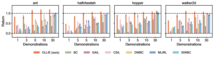
Figure 25: End-to-end performance from offline pretraining to 10-episode finetuning under varying quantities of expert trajectories in MuJoCo. Uncertainty intervals depict standard deviation over five seeds. The results demonstrate OLLIE’s overall efficiency in both sampling/interaction and expert demonstrations, and underscore the great potential of pretraining and fintuning paradigm in IL.

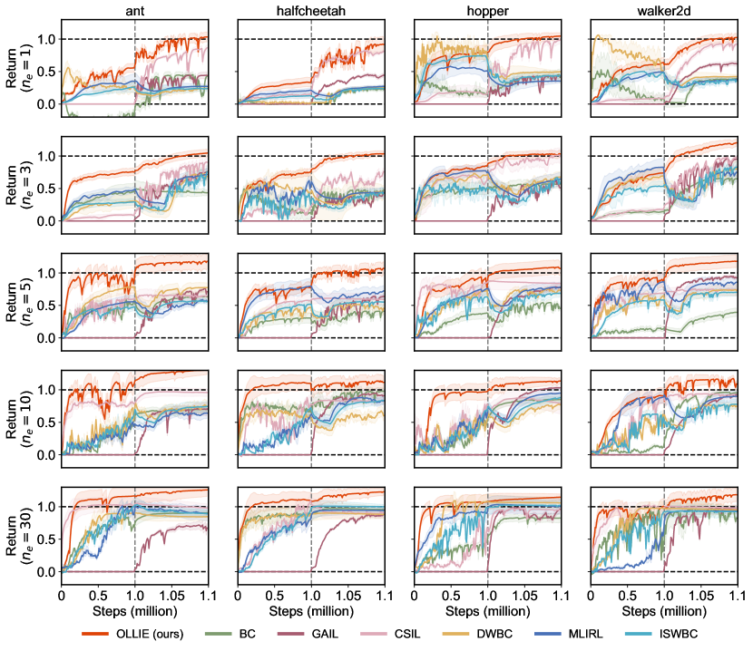
Figure 26: End-to-end learning curves from offline pretraining to online finetuning under varying quantities of expert trajectories in MuJoCo. The dashed line separates the offline and online phases. Uncertainty intervals depict standard deviation over five seeds. $n_{e}$ represents expert trajectories. The simple combination of existing offline IL and GAIL suffers from unlearning pretrained knowledge. OLLIE not only avoids this issue but also expedites online training. This is attributed to OLLIE’s initial discriminator aligning with the well-performed policy initialization, thereby acting as a good local reward function capable of guiding fast policy search. In addition, while CSIL can alleviate the unlearning issue to some extent, its IRL procesure exhibits inefficiency compared to OLLIE.

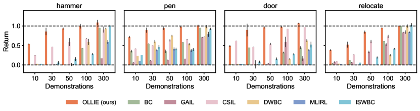
Figure 27: End-to-end performance from offline pretraining to 10-episode finetuning under varying quantities of expert trajectories in Adroit. Uncertainty intervals depict standard deviation over five seeds. The results demonstrate OLLIE’s remarkable overall efficiency in both sampling/interaction and expert demonstrations and underscore the great potential of pretraining and fintuning paradigm in IL.

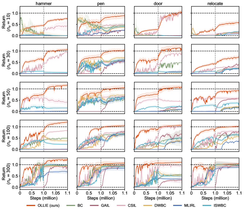
Figure 28: End-to-end learning curves from offline pretraining to online finetuning under varying quantities of expert trajectories in Adroit. Uncertainty intervals depict standard deviation over five seeds. $n_{e}$ represents expert trajectories. Simple combination of existing offline IL and GAIL suffers from unlearning pretrained knowledge. OLLIE not only avoids this issue but also expedites online training. This is attributed to OLLIE’s initial discriminator aligning with the well-performed policy initialization, thereby acting as a good local reward function capable of guiding fast policy search. In comparison with MuJoCo, high-dimensional environments make reward learning more challenging for IRL methods.

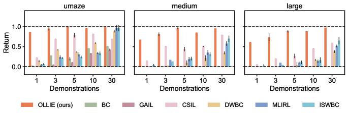
Figure 29: End-to-end performance from offline pretraining to 10-episode finetuning under varying quantities of expert trajectories in AntMaze. Uncertainty intervals depict standard deviation over five seeds. It demonstrates the remarkable overall efficiency of OLLIE in both sampling/interaction and expert demonstrations and underscores great potentials of the pretraining and fintuning paradigm in IL.

Figure 30: End-to-end learning curves from offline pretraining to online finetuning under varying quantities of expert trajectories in AntMaze. Uncertainty intervals depict standard deviation over five seeds. $n_{e}$ represents expert trajectories. The simple combination of existing offline IL and GAIL suffers from unlearning pretrained knowledge. OLLIE not only avoids this issue but also expedites online training. This is attributed to OLLIE’s initial discriminator aligning with the well-performed policy initialization, thereby acting as a good local reward function capable of guiding fast policy search. Importantly, in the medium and large layouts, GAIL from scratch fails even with sufficient expert demonstrations. This may stem from the ineffective exploration of random policies in this domain, revealing the significance of effective pretraining in IL.

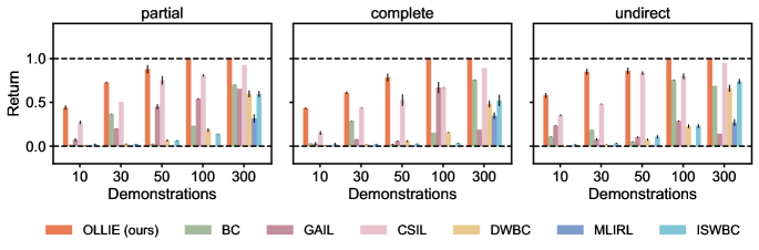
Figure 31: End-to-end performance from offline pretraining to 10-episode finetuning under varying quantities of expert trajectories in FrankaKitchen. Uncertainty intervals depict standard deviation over five seeds. The results clearly demonstrate the remarkable overall efficiency of OLLIE in both sampling/interaction and expert demonstrations and underscore the great potential of pretraining and fintuning paradigm in IL.

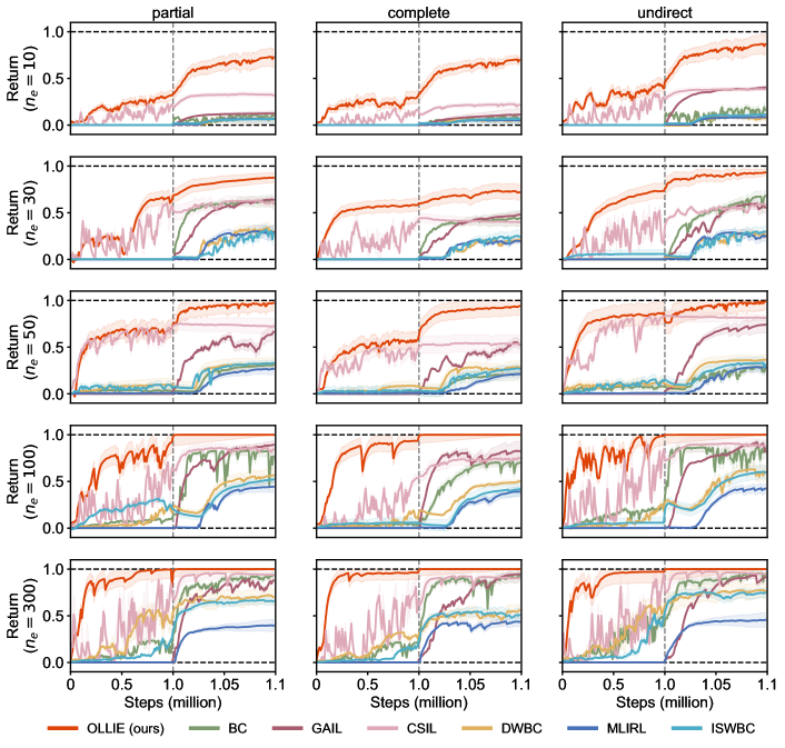
Figure 32: End-to-end learning curves from offline pretraining to online finetuning under varying quantities of expert trajectories in FrankaKitchen. Uncertainty intervals depict standard deviation over five seeds. $n_{e}$ represents expert trajectories. The simple combination of existing offline IL and GAIL suffers from unlearning pretrained knowledge. OLLIE not only avoids this issue but also expedites online training. This is attributed to OLLIE’s initial discriminator aligning with the well-performed policy initialization, thereby acting as a good local reward function capable of guiding fast policy search. In comparison with MuJoCo, high-dimensional environments make reward learning more challenging for IRL methods.

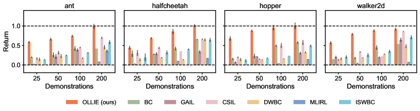
Figure 33: End-to-end performance from offline pretraining to 10-episode finetuning under varying quantities of expert trajectories in vision-based MuJoCo. Uncertainty intervals depict standard deviation over five seeds. The results clearly demonstrate the remarkable overall efficiency of OLLIE in both sampling/interaction in high-dimensional environments and expert demonstrations and underscore the great practical potential of pretraining and fintuning paradigm in IL.

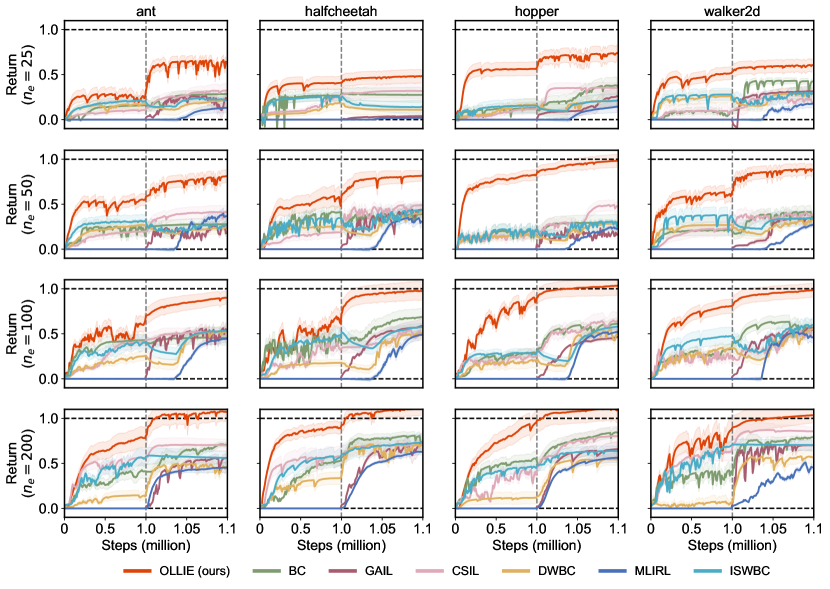
Figure 34: End-to-end learning curves from offline pretraining to online finetuning under varying quantities of expert trajectories in vision-based MuJoCo. Uncertainty intervals depict standard deviation over five seeds. $n_{e}$ represents expert trajectories. The simple combination of existing offline IL and GAIL suffers from unlearning pretrained knowledge. OLLIE not only avoids this issue but also expedites online training. This is attributed to OLLIE’s initial discriminator aligning with the well-performed policy initialization, thereby acting as a good local reward function capable of guiding fast policy search. The superiority of OLLIE proves more remarkable in this vision-based domain, demonstrating its promise in practical scenarios.

Figure 35: End-to-end performance from offline pretraining to 10-episode finetuning under varying quantities of expert trajectories in vision-based Robomimic. Uncertainty intervals depict standard deviation over five seeds. The results demonstrate the remarkable overall efficiency of OLLIE in both sampling/interaction in high-dimensional environments and expert demonstrations and underscore the great practical potential of pretraining and fintuning paradigm in IL.

G.3 Ablation Studies and Complementary Experiments

This section includes ablation studies for OLLIE and complementary empirical studies.

G.3.1 Importance of discriminator initialization

We ablate the discriminator initialization by a random initialization and run experiments with the same setup as Tables 15, 18 and 20. Not surprisingly, albeit with a good policy initialization, the finetuning performance degrades dramatically in the absence of the initialized discriminator. In addition, Fig. 37 demonstrates that pretraining with less expert demonstrations leads to a worse finetuning performance. This could be attributed to the poor generalizability of the policy trained with less data (akin to the findings of He et al. (2019) in vision).

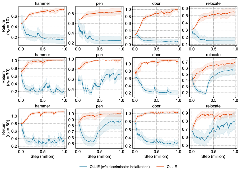
Figure 37: Ablation on the discriminator initialization. Uncertainty intervals depict standard deviation over five seeds. Albeit with a good policy initialization, the finetuning performance of OLLIE experiences a significant degradation in the absence of the initialized discriminator.

G.3.2 Importance of Imperfect Demonstrations

To assess the effect of imperfect demonstrations, we carry out experiments by varying the number of complementary trajectories from 0 to 1000. The setup follows that of Tables 15, 18 and 20. As illustrated in Fig. 38, it is important to incorporate complementary data, which can remedy the limited state coverage of expert demonstrations and combat covariate shifts. Moreover, with no complementary data, DWBC, ISWBC, and CSIL reduce to BC or soft BC, which proves ineffective with scarce expert data; and the model-based counterparts struggle in these high-dimensional environments. In contrast, OLLIE works much better, as it can effectively leverage the dynamics information in expert demonstrations and enable the policy to stay in the expert data support as much as possible.

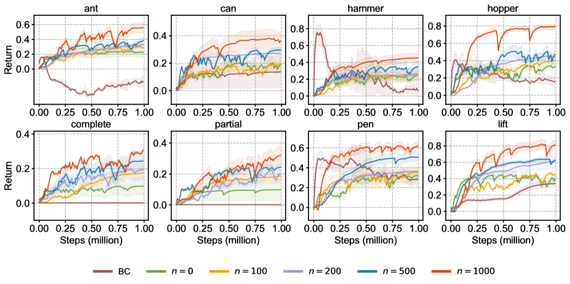
Figure 38: Importance of complementary suboptimal data. Uncertainty intervals depict standard deviation over five seeds. Even with no complementary data, OLLIE outperforms BC, owing to the capability of utilizing dynamics information in expert demonstrations.

G.3.3 A Visualization of Distribution Matching

To validate the theory of OLLIE where it minimizes the discrepancy with the empirical expert distribution, we visualize the experimental result of antmaze-large in Fig. 39, where OLLIE nearly recovers the expert state-action distribution. From Eq. (5) of Xu et al. (2022a), DWBC assigns positive weights to all diverse state-actions, leading to the interference in mimicking expert behaviors. As analyzed in Appendix A, with scarce expert data, ISWBC may pursue a biased objective and suffer from error compounding once leaving the expert data support.

(a) Expert data

(b) Imperfect data

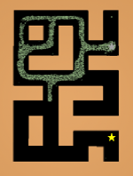
(c) DWBC

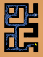
(d) ISWBC

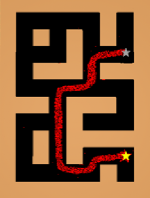
(e) OLLIE

Figure 39: Visualization of the trajectories in antmaze-large generated by different algorithms. The policies are trained with 10 expert trajectory (shown in (a)) as the expert demonstration and 1000 diverse trajectories (shown in (b)) as imperfect demonstrations. (c)-(d) depict the trajectories sampled from the policies learned by DWBC, ISWBC, and OLLIE, repectively.

G.3.4 Minimax Optimization

We test the stability of the approximate dual descent in solving the SSP. As shown in Fig. 40, it works well in all environments and often converges in 50k gradient steps.

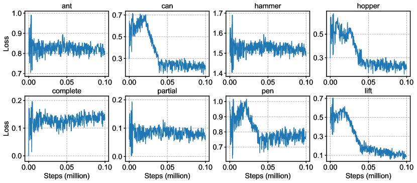
Figure 40: The value of $\tilde{F}(\phi_{\nu},\phi_{y})$ in selected experiments.

G.3.5 Further Comparison with MLIRL

In our experiments, we use GAIL to tune the policy learned by MLIRL. Since MLIRL learns a reward function during the offline phase, another approach to tune MLIRL is employing forward RL with the learning reward function. Unfortunately, we find it performs highly suboptimally, as demonstrated in Fig. 41. This is because the reward extrapolation error leads to spurious rewards in out-of-distribution environments. Of note, despite being an IRL method, CSIL can alleviate this issue to some extent by further refining the reward function during online fine-tuning.

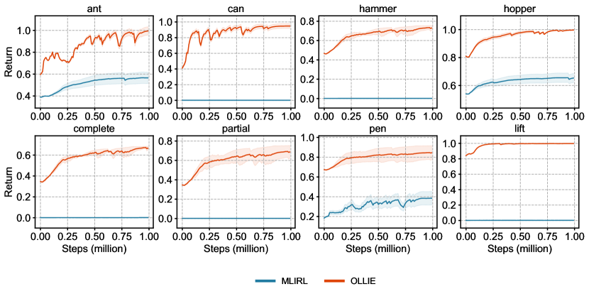
Figure 41: Performance of finetuning MLIRL via its learned reward function. Uncertainty intervals depict standard deviation over five seeds.

G.3.6 Undiscounted Experiments

As discussed in Appendix D, OLLIE can extend to undiscounted problems ($\gamma=1$). In Fig. 42, we compare between discounted and undiscounted OLLIE. There is not a significant discrepancy between them across employed benchmarks.

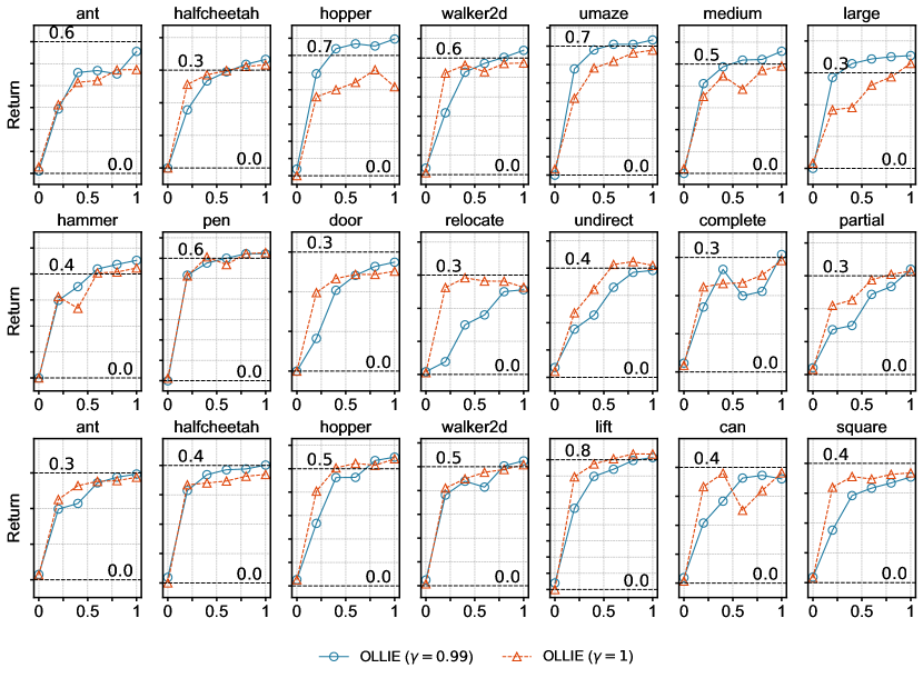
Figure 42: Performance of discounted and discounted OLLIE in offline IL. The results are averaged over 5 random seeds. The last row comprises vision-based tasks.

G.3.7 Forward and Reverse Policy Extraction

We examine the performance of the forward and reverse policy extraction methods introduced in Section 5.4. The setup remains the same as Tables 15, 18 and 20 with limited expert demonstrations and low-quality complementary data. They both work well in the benchmarks, of which the final performance is environment-dependent. We find the forward method enjoys better convergence speed and stability in most environments.

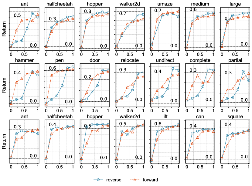
Figure 43: Comparison between the forward and reverse policy extraction. Uncertainty intervals depict standard deviation over five seeds. The forward method enjoys better convergence speed and stability in most environments. Their final performance is environment-dependent.

G.3.8 Discriminator Alignment

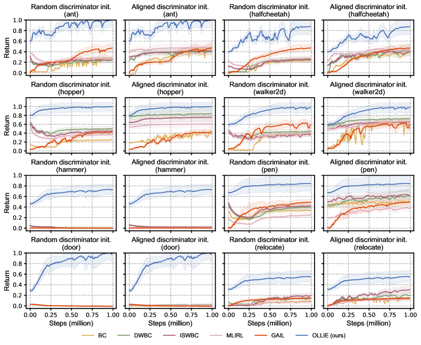
Figure 44: The effect of discriminator alignment. Uncertainty intervals depict standard deviation over five random seeds. In each task, the left figure depicts the performance of finetuning the policies learned by existing methods using GAIL with a random discriminator initialization. The right figure shows the performance after aligning the discriminator using 100 trajectories generated by the initialized policies. In MuJoCo, the policies are pretrained with 1 expert trajectory and 1000 random trajectories. In Adroit, the policies are pretrained with 10 expert trajectory and 1000 cloned trajectories.

References

- Abbeel & Ng (2004) Abbeel, P. and Ng, A. Y. Apprenticeship learning via inverse reinforcement learning. In Proceedings of the 21st International Conference on Machine Learning, pp. 1. ACM, 2004.
- Al-Hafez et al. (2023) Al-Hafez, F., Tateo, D., Arenz, O., Zhao, G., and Peters, J. LS-IQ: Implicit reward regularization for inverse reinforcement learning. In International Conference on Learning Representations, 2023.
- Arora & Doshi (2021) Arora, S. and Doshi, P. A survey of inverse reinforcement learning: Challenges, methods and progress. Artificial Intelligence, 297:103500, 2021.
- Ball et al. (2023) Ball, P. J., Smith, L., Kostrikov, I., and Levine, S. Efficient online reinforcement learning with offline data. In Proceedings of the 40th International Conference on Machine Learning, volume 202, pp. 1577–1594. PMLR, 2023.
- Barde et al. (2020) Barde, P., Roy, J., Jeon, W., Pineau, J., Pal, C., and Nowrouzezahrai, D. Adversarial soft advantage fitting: Imitation learning without policy optimization. In Advances in Neural Information Processing Systems, volume 33, pp. 12334–12344. Curran Associates, 2020.
- Bertsekas et al. (2003) Bertsekas, D., Nedic, A., and Ozdaglar, A. Convex analysis and optimization, volume 1. Athena Scientific, 2003.
- Blondé & Kalousis (2019) Blondé, L. and Kalousis, A. Sample-efficient imitation learning via generative adversarial nets. In Proceedings of the 22nd International Conference on Artificial Intelligence and Statistics, volume 89, pp. 3138–3148. PMLR, 2019.
- Boyd & Vandenberghe (2004) Boyd, S. P. and Vandenberghe, L. Convex optimization. Cambridge university press, 2004.
- Brantley et al. (2020) Brantley, K., Sun, W., and Henaff, M. Disagreement-regularized imitation learning. In International Conference on Learning Representations, 2020.
- Brown et al. (2020) Brown, T., Mann, B., Ryder, N., Subbiah, M., Kaplan, J. D., Dhariwal, P., Neelakantan, A., Shyam, P., Sastry, G., Askell, A., et al. Language models are few-shot learners. In Proceedings of Advances in Neural Information Processing Systems, pp. 1877–1901, 2020.
- Chan & van der Schaar (2021) Chan, A. J. and van der Schaar, M. Scalable bayesian inverse reinforcement learning. In International Conference on Learning Representations, 2021.
- Chang et al. (2021) Chang, J., Uehara, M., Sreenivas, D., Kidambi, R., and Sun, W. Mitigating covariate shift in imitation learning via offline data with partial coverage. In Advances in Neural Information Processing Systems, volume 34, pp. 965–979. Curran Associates, 2021.
- Chen et al. (2019) Chen, M., Wang, Y., Liu, T., Yang, Z., Li, X., Wang, Z., and Zhao, T. On computation and generalization of generative adversarial imitation learning. In International Conference on Learning Representations, 2019.
- Choi & Kim (2013) Choi, J. and Kim, K.-E. Bayesian nonparametric feature construction for inverse reinforcement learning. In Proceedings of the 23rd International Joint Conference on Artificial Intelligence, pp. 1287–1293. AAAI Press, 2013.
- Cideron et al. (2023) Cideron, G., Tabanpour, B., Curi, S., Girgin, S., Hussenot, L., Dulac-Arnold, G., Geist, M., Pietquin, O., and Dadashi, R. Get back here: Robust imitation by return-to-distribution planning. arXiv preprint arXiv:2305.01400, 2023.
- Dadashi et al. (2021) Dadashi, R., Hussenot, L., Geist, M., and Pietquin, O. Primal wasserstein imitation learning. In International Conference on Learning Representations, 2021.
- Ding et al. (2019) Ding, Y., Florensa, C., Abbeel, P., and Phielipp, M. Goal-conditioned imitation learning. In Advances in Neural Information Processing Systems, volume 32, pp. 15324–15335. Curran Associates, 2019.
- Du & Pardalos (1995) Du, D.-Z. and Pardalos, P. M. Minimax and applications, volume 4. Springer Science & Business Media, 1995.
- Finn et al. (2016) Finn, C., Levine, S., and Abbeel, P. Guided cost learning: Deep inverse optimal control via policy optimization. In Proceedings of the 33rd International Conference on Machine Learning, volume 48, pp. 49–58. PMLR, 2016.
- Florence et al. (2022) Florence, P., Lynch, C., Zeng, A., Ramirez, O. A., Wahid, A., Downs, L., Wong, A., Lee, J., Mordatch, I., and Tompson, J. Implicit behavioral cloning. In Proceedings of the 5th Conference on Robot Learning, volume 164, pp. 158–168. PMLR, 2022.
- Fu et al. (2018) Fu, J., Luo, K., and Levine, S. Learning robust rewards with adverserial inverse reinforcement learning. In International Conference on Learning Representations, 2018.
- Fu et al. (2020) Fu, J., Kumar, A., Nachum, O., Tucker, G., and Levine, S. D4RL: Datasets for deep data-driven reinforcement learning. arXiv preprint arXiv:2004.07219, 2020.
- Fujimoto & Gu (2021) Fujimoto, S. and Gu, S. S. A minimalist approach to offline reinforcement learning. In Advances in Neural Information Processing Systems, volume 34, pp. 20132–20145. Curran Associates, 2021.
- Garg et al. (2021) Garg, D., Chakraborty, S., Cundy, C., Song, J., and Ermon, S. IQ-Learn: Inverse soft-q learning for imitation. In Advances in Neural Information Processing Systems, volume 34, pp. 4028–4039. Curran Associates, 2021.
- Ghasemipour et al. (2020) Ghasemipour, S. K. S., Zemel, R., and Gu, S. A divergence minimization perspective on imitation learning methods. In Proceedings of the 3rd Conference on Robot Learning, volume 100, pp. 1259–1277. PMLR, 2020.
- Goodfellow et al. (2014) Goodfellow, I., Pouget-Abadie, J., Mirza, M., Xu, B., Warde-Farley, D., Ozair, S., Courville, A., and Bengio, Y. Generative adversarial nets. In Advances in Neural Information Processing Systems, volume 27, pp. 2672–2680. Curran Associates, 2014.
- Guan et al. (2021) Guan, Z., Xu, T., and Liang, Y. When will generative adversarial imitation learning algorithms attain global convergence. In Proceedings of The 24th International Conference on Artificial Intelligence and Statistics, volume 130, pp. 1117–1125. PMLR, 2021.
- Gupta et al. (2019) Gupta, A., Kumar, V., Lynch, C., Levine, S., and Hausman, K. Relay policy learning: Solving long-horizon tasks via imitation and reinforcement learning. arXiv preprint arXiv:1910.11956, 2019.
- Haarnoja et al. (2018) Haarnoja, T., Zhou, A., Abbeel, P., and Levine, S. Soft actor-critic: Off-policy maximum entropy deep reinforcement learning with a stochastic actor. In Proceedings of the 35th International Conference on Machine Learning, volume 80, pp. 1861–1870. PMLR, 2018.
- He et al. (2019) He, K., Girshick, R., and Dollár, P. Rethinking ImageNet pre-training. In Proceedings of the IEEE/CVF International Conference on Computer Vision, pp. 4918–4927, 2019.
- He et al. (2022) He, K., Chen, X., Xie, S., Li, Y., Dollár, P., and Girshick, R. Masked autoencoders are scalable vision learners. In Proceedings of the IEEE/CVF conference on computer vision and pattern recognition, pp. 16000–16009, 2022.
- Ho & Ermon (2016) Ho, J. and Ermon, S. Generative adversarial imitation learning. In Advances in Neural Information Processing Systems, volume 29, pp. 4572–4580. Curran Associates, 2016.
- Hussein et al. (2017) Hussein, A., Gaber, M. M., Elyan, E., and Jayne, C. Imitation learning: A survey of learning methods. ACM Computing Survey, 50(2):1–35, 2017.
- Jarrett et al. (2020) Jarrett, D., Bica, I., and van der Schaar, M. Strictly batch imitation learning by energy-based distribution matching. In Advances in Neural Information Processing Systems, volume 33, pp. 7354–7365. Curran Associates, 2020.
- Jena et al. (2021) Jena, R., Liu, C., and Sycara, K. Augmenting GAIL with BC for sample efficient imitation learning. In Proceedings of the 4th Conference on Robot Learning, pp. 80–90. PMLR, 2021.
- Ke et al. (2021) Ke, L., Choudhury, S., Barnes, M., Sun, W., Lee, G., and Srinivasa, S. Imitation learning as -divergence minimization. In Algorithmic Foundations of Robotics XIV, pp. 313–329. Springer, 2021.
- Kim et al. (2022a) Kim, G.-H., Lee, J., Jang, Y., Yang, H., and Kim, K.-E. LobsDICE: Offline learning from observation via stationary distribution correction estimation. In Advances in Neural Information Processing Systems, volume 35, pp. 8252–8264. Curran Associates, 2022a.
- Kim et al. (2022b) Kim, G.-H., Seo, S., Lee, J., Jeon, W., Hwang, H., Yang, H., and Kim, K.-E. DemoDICE: Offline imitation learning with supplementary imperfect demonstrations. In International Conference on Learning Representations, 2022b.
- Kostrikov et al. (2018) Kostrikov, I., Agrawal, K. K., Dwibedi, D., Levine, S., and Tompson, J. Discriminator-actor-critic: Addressing sample inefficiency and reward bias in adversarial imitation learning. In International Conference on Learning Representations, 2018.
- Kostrikov et al. (2020) Kostrikov, I., Nachum, O., and Tompson, J. Imitation learning via off-policy distribution matching. In International Conference on Learning Representations, 2020.
- Kuefler et al. (2017) Kuefler, A., Morton, J., Wheeler, T., and Kochenderfer, M. Imitating driver behavior with generative adversarial networks. In Proceedings of the 28th IEEE Intelligent Vehicles Symposium, pp. 204–211. IEEE, 2017.
- Kumar et al. (2020) Kumar, A., Zhou, A., Tucker, G., and Levine, S. Conservative q-learning for offline reinforcement learning. In Advances in Neural Information Processing Systems, volume 33, pp. 1179–1191. Curran Associates, 2020.
- Lee et al. (2019) Lee, D., Srinivasan, S., and Doshi-Velez, F. Truly batch apprenticeship learning with deep successor features. In Proceedings of the 28th International Joint Conference on Artificial Intelligence, pp. 5909–5915, 2019.
- Lee et al. (2021) Lee, J., Jeon, W., Lee, B., Pineau, J., and Kim, K.-E. OptiDICE: Offline policy optimization via stationary distribution correction estimation. In Proceedings of the 38th International Conference on Machine Learning, volume 139, pp. 6120–6130. PMLR, 2021.
- Lee et al. (2022) Lee, S., Seo, Y., Lee, K., Abbeel, P., and Shin, J. Offline-to-online reinforcement learning via balanced replay and pessimistic Q-ensemble. In Proceedings of the 5th Conference on Robot Learning, volume 164, pp. 1702–1712. PMLR, 2022.
- Levine et al. (2010) Levine, S., Popovic, Z., and Koltun, V. Feature construction for inverse reinforcement learning. In Advances in Neural Information Processing Systems, volume 23, pp. 1342–1350. Curran Associates, 2010.
- Levine et al. (2011) Levine, S., Popovic, Z., and Koltun, V. Nonlinear inverse reinforcement learning with Gaussian processes. In Advances in Neural Information Processing Systems, volume 24, pp. 19–27. Curran Associates, 2011.
- Li et al. (2023a) Li, Q., Zhang, J., Ghosh, D., Zhang, A., and Levine, S. Accelerating exploration with unlabeled prior data. In The 37th Conference on Neural Information Processing Systems, 2023a.
- Li et al. (2017) Li, Y., Song, J., and Ermon, S. InfoGAIL: Interpretable imitation learning from visual demonstrations. In Advances in Neural Information Processing Systems, volume 30, pp. 3815–3825. Curran Associates, 2017.
- Li et al. (2023b) Li, Z., Xu, T., Qin, Z., Yu, Y., and Luo, Z.-Q. Imitation learning from imperfection: Theoretical justifications and algorithms. In The 37th Conference on Neural Information Processing Systems, 2023b.
- Ma et al. (2022) Ma, Y., Shen, A., Jayaraman, D., and Bastani, O. Versatile offline imitation from observations and examples via regularized state-occupancy matching. In Proceedings of the 39th International Conference on Machine Learning, volume 162, pp. 14639–14663. PMLR, 2022.
- Mandlekar et al. (2022) Mandlekar, A., Xu, D., Wong, J., Nasiriany, S., Wang, C., Kulkarni, R., Fei-Fei, L., Savarese, S., Zhu, Y., and Martín-Martín, R. What matters in learning from offline human demonstrations for robot manipulation. In Proceedings of the 5th Conference on Robot Learning, volume 164, pp. 1678–1690. PMLR, 2022.
- Mark et al. (2022) Mark, M. S., Ghadirzadeh, A., Chen, X., and Finn, C. Fine-tuning offline policies with optimistic action selection. In NeurIPS Workshop on Deep Reinforcement Learning, 2022.
- Nachum et al. (2019a) Nachum, O., Chow, Y., Dai, B., and Li, L. DualDICE: Behavior-agnostic estimation of discounted stationary distribution corrections. In Advances in Neural Information Processing Systems, volume 32, pp. 2318–2328. Curran Associates, 2019a.
- Nachum et al. (2019b) Nachum, O., Dai, B., Kostrikov, I., Chow, Y., Li, L., and Schuurmans, D. AlgaeDICE: Policy gradient from arbitrary experience. arXiv preprint arXiv:1912.02074, 2019b.
- Nakamoto et al. (2023) Nakamoto, M., Zhai, Y., Singh, A., Ma, Y., Finn, C., Kumar, A., and Levine, S. Cal-QL: Calibrated offline rl pre-training for efficient online fine-tuning. In The 37th Conference on Neural Information Processing Systems, 2023.
- Nemirovski (2004) Nemirovski, A. Prox-method with rate of convergence for variational inequalities with Lipschitz continuous monotone operators and smooth convex-concave saddle point problems. SIAM Journal on Optimization, 15(1):229–251, 2004.
- Ng & Russell (2000) Ng, A. Y. and Russell, S. J. Algorithms for inverse reinforcement learning. In Proceedings of the 17th International Conference on Machine Learning, pp. 663–670. Morgan Kaufmann, 2000.
- Ni et al. (2021) Ni, T., Sikchi, H., Wang, Y., Gupta, T., Lee, L., and Eysenbach, B. -IRL: Inverse reinforcement learning via state marginal matching. In Proceedings of the 4th Conference on Robot Learning, pp. 529–551. PMLR, 2021.
- Orsini et al. (2021) Orsini, M., Raichuk, A., Hussenot, L., Vincent, D., Dadashi, R., Girgin, S., Geist, M., Bachem, O., Pietquin, O., and Andrychowicz, M. What matters for adversarial imitation learning? In Advances in Neural Information Processing Systems, volume 34, pp. 14656–14668. Curran Associates, 2021.
- Osa et al. (2018) Osa, T., Pajarinen, J., Neumann, G., Bagnell, J. A., Abbeel, P., Peters, J., et al. An algorithmic perspective on imitation learning. Foundations and Trends in Robotics, 7(1-2):1–179, 2018.
- Pomerleau (1988) Pomerleau, D. A. ALVINN: An autonomous land vehicle in a neural network. In Advances in Neural Information Processing Systems, volume 1, pp. 305–313. Morgan Kaufmann, 1988.
- Puterman (2014) Puterman, M. L. Markov decision processes: discrete stochastic dynamic programming. John Wiley & Sons, 2014.
- Rafailov et al. (2023) Rafailov, R., Sharma, A., Mitchell, E., Ermon, S., Manning, C. D., and Finn, C. Direct preference optimization: Your language model is secretly a reward model. In The 37th Conference on Neural Information Processing Systems, 2023.
- Rajaraman et al. (2020) Rajaraman, N., Yang, L., Jiao, J., and Ramchandran, K. Toward the fundamental limits of imitation learning. In Advances in Neural Information Processing Systems, volume 33, pp. 2914–2924. Curran Associates, 2020.
- Rajeswaran et al. (2017) Rajeswaran, A., Kumar, V., Gupta, A., Vezzani, G., Schulman, J., Todorov, E., and Levine, S. Learning complex dexterous manipulation with deep reinforcement learning and demonstrations. arXiv preprint arXiv:1709.10087, 2017.
- Ratliff et al. (2006) Ratliff, N. D., Bagnell, J. A., and Zinkevich, M. A. Maximum margin planning. In Proceedings of the 23rd International Conference on Machine Learning, pp. 729–736. ACM, 2006.
- Reddy et al. (2019) Reddy, S., Dragan, A. D., and Levine, S. SQIL: Imitation learning via reinforcement learning with sparse rewards. In International Conference on Learning Representations, 2019.
- Ross & Bagnell (2010) Ross, S. and Bagnell, D. Efficient reductions for imitation learning. In Proceedings of the 13th International Conference on Artificial Intelligence and Statistics, volume 9, pp. 661–668. PMLR, 2010.
- Russell (1998) Russell, S. Learning agents for uncertain environments (extended abstract). In Proceedings of the 7th Annual Conference on Computational Learning Theory, pp. 101–103. ACM, 1998.
- Sammut et al. (1992) Sammut, C., Hurst, S., Kedzier, D., and Michie, D. Learning to fly. In Machine Learning Proceedings 1992, pp. 385–393. Morgan Kaufmann, 1992.
- Sasaki & Yamashina (2021) Sasaki, F. and Yamashina, R. Behavioral cloning from noisy demonstrations. In International Conference on Learning Representations, 2021.
- Sasaki et al. (2019) Sasaki, F., Yohira, T., and Kawaguchi, A. Sample efficient imitation learning for continuous control. In International conference on learning representations, 2019.
- Song et al. (2022) Song, Y., Zhou, Y., Sekhari, A., Bagnell, D., Krishnamurthy, A., and Sun, W. Hybrid RL: Using both offline and online data can make RL efficient. In International Conference on Learning Representations, 2022.
- Sun et al. (2021) Sun, M., Mahajan, A., Hofmann, K., and Whiteson, S. SoftDICE for imitation learning: Rethinking off-policy distribution matching. arXiv preprint arXiv:2106.03155, 2021.
- Swamy et al. (2021a) Swamy, G., Choudhury, S., Bagnell, J. A., and Wu, S. Of moments and matching: A game-theoretic framework for closing the imitation gap. In Proceedings of the 38th International Conference on Machine Learning, volume 139, pp. 10022–10032. PMLR, 2021a.
- Swamy et al. (2021b) Swamy, G., Choudhury, S., Bagnell, J. A., and Wu, Z. S. A critique of strictly batch imitation learning. arXiv preprint arXiv:2110.02063, 2021b.
- Syed & Schapire (2007) Syed, U. and Schapire, R. E. A game-theoretic approach to apprenticeship learning. In Advances in Neural Information Processing Systems, volume 20, pp. 1449–1456. Curran Associates, 2007.
- Syed et al. (2008) Syed, U., Bowling, M., and Schapire, R. E. Apprenticeship learning using linear programming. In Proceedings of the 25th International Conference on Machine Learning, pp. 1032–1039. ACM, 2008.
- Viano et al. (2022) Viano, L., Kamoutsi, A., Neu, G., Krawczuk, I., and Cevher, V. Proximal point imitation learning. In Advances in Neural Information Processing Systems, volume 35, pp. 24309–24326. Curran Associates, 2022.
- Wagenmaker & Pacchiano (2023) Wagenmaker, A. and Pacchiano, A. Leveraging offline data in online reinforcement learning. In Proceedings of the 40th International Conference on Machine Learning, volume 202, pp. 35300–35338. PMLR, 2023.
- Wang et al. (2023a) Wang, H., Lin, S., and Zhang, J. Warm-start actor-critic: From approximation error to sub-optimality gap. In Proceedings of the 40th International Conference on Machine Learning, volume 202, pp. 35989–36019. PMLR, 2023a.
- Wang et al. (2018) Wang, Q., Xiong, J., Han, L., sun, p., Liu, H., and Zhang, T. Exponentially weighted imitation learning for batched historical data. In Advances in Neural Information Processing Systems, volume 31, pp. 6291–6300. Curran Associates, 2018.
- Wang et al. (2019) Wang, R., Ciliberto, C., Amadori, P. V., and Demiris, Y. Random expert distillation: Imitation learning via expert policy support estimation. In Proceedings of the 36th International Conference on Machine Learning, volume 97, pp. 6536–6544. PMLR, 2019.
- Wang et al. (2023b) Wang, S., Yang, Q., Gao, J., Lin, M. G., CHEN, H., Wu, L., Jia, N., Song, S., and Huang, G. Train once, get a family: State-adaptive balances for offline-to-online reinforcement learning. In The 37th Conference on Neural Information Processing Systems, 2023b.
- Watson et al. (2024) Watson, J., Huang, S., and Heess, N. Coherent soft imitation learning. In Advances in Neural Information Processing Systems, volume 36, pp. 14540–14583. Curran Associates, 2024.
- Xu et al. (2022a) Xu, H., Zhan, X., Yin, H., and Qin, H. Discriminator-weighted offline imitation learning from suboptimal demonstrations. In Proceedings of the 39th International Conference on Machine Learning, volume 162, pp. 24725–24742. PMLR, 2022a.
- Xu et al. (2022b) Xu, T., Li, Z., Yu, Y., and Luo, Z.-Q. Understanding adversarial imitation learning in small sample regime: A stage-coupled analysis. arXiv preprint arXiv:2208.01899, 2022b.
- Yang et al. (2023) Yang, H., Yu, C., Chen, S., et al. Hybrid policy optimization from imperfect demonstrations. In The 37th Conference on Neural Information Processing Systems, 2023.
- Yu et al. (2023) Yu, L., Yu, T., Song, J., Neiswanger, W., and Ermon, S. Offline imitation learning with suboptimal demonstrations via relaxed distribution matching. In Proceedings of the AAAI Conference on Artificial Intelligence, volume 37, pp. 11016–11024. AAAI Press, 2023.
- Yu et al. (2022) Yu, T., Kumar, A., Chebotar, Y., Hausman, K., Finn, C., and Levine, S. How to leverage unlabeled data in offline reinforcement learning. In Proceedings of the 39th International Conference on Machine Learning, volume 162, pp. 25611–25635. PMLR, 2022.
- Yue et al. (2023) Yue, S., Wang, G., Shao, W., Zhang, Z., Lin, S., Ren, J., and Zhang, J. CLARE: Conservative model-based reward learning for offline inverse reinforcement learning. In International Conference on Learning Representations, 2023.
- Yue et al. (2024) Yue, S., Deng, Y., Wang, G., Ren, J., and Zhang, Y. Federated offline reinforcement learning with proximal policy evaluation. Chinese Journal of Electronics, 33(6):1–13, 2024.
- Zeng et al. (2022) Zeng, S., Li, C., Garcia, A., and Hong, M. Maximum-likelihood inverse reinforcement learning with finite-time guarantees. In Advances in Neural Information Processing Systems, volume 35, pp. 10122–10135. Curran Associates, 2022.
- Zeng et al. (2023) Zeng, S., Li, C., Garcia, A., and Hong, M. When demonstrations meet generative world models: A maximum likelihood framework for offline inverse reinforcement learning. In The 37th Conference on Neural Information Processing Systems, 2023.
- Zhang et al. (2021) Zhang, J., Hong, M., Wang, M., and Zhang, S. Generalization bounds for stochastic saddle point problems. In Proceedings of the 24th International Conference on Artificial Intelligence and Statistics, pp. 568–576. PMLR, 2021.
- Zhang & Zanette (2023) Zhang, R. and Zanette, A. Policy finetuning in reinforcement learning via design of experiments using offline data. In The 37th Conference on Neural Information Processing Systems, 2023.
- Zhang et al. (2020) Zhang, Y., Cai, Q., Yang, Z., and Wang, Z. Generative adversarial imitation learning with neural network parameterization: Global optimality and convergence rate. In Proceedings of the 37th International Conference on Machine Learning, volume 119, pp. 11044–11054. PMLR, 2020.
- Ziebart et al. (2008) Ziebart, B. D., Maas, A., Bagnell, J. A., and Dey, A. K. Maximum entropy inverse reinforcement learning. In Proceedings of the 23rd National Conference on Artificial Intelligence, pp. 1433–1438. AAAI Press, 2008.
- Zolna et al. (2020) Zolna, K., Novikov, A., Konyushkova, K., Gulcehre, C., Wang, Z., Aytar, Y., Denil, M., de Freitas, N., and Reed, S. Offline learning from demonstrations and unlabeled experience. In NeurIPS Workshop on Offline Reinforcement Learning, 2020.
- Zou et al. (2018) Zou, H., Su, H., Song, S., and Zhu, J. Understanding human behaviors in crowds by imitating the decision-making process. In Proceedings of the AAAI Conference on Artificial Intelligence, volume 32, pp. 7648–7655. AAAI Press, 2018.