Optimized Linear Measurements for Inverse Problems using Diffusion-Based Image Generation

Abstract

We re-examine the problem of reconstructing a high-dimensional signal from a small set of linear measurements, in combination with image prior from a diffusion probabilistic model. Well-established methods for optimizing such measurements include principal component analysis (PCA), independent component analysis (ICA) and compressed sensing (CS), all of which rely on axis- or subspace-aligned statistical characterization. But many naturally occurring signals, including photographic images, contain richer statistical structure. To exploit such structure, we introduce a general method for obtaining an optimized set of linear measurements, assuming a Bayesian inverse solution that leverages the prior implicit in a neural network trained to perform denoising. We demonstrate that these measurements are distinct from those of PCA and CS, with significant improvements in minimizing squared reconstruction error. In addition, we show that optimizing the measurements for the SSIM perceptual loss leads to perceptually improved reconstruction. Our results highlight the importance of incorporating the specific statistical regularities of natural signals when designing effective linear measurements.

1 Introduction

Natural signals, such as images and videos, are typically acquired in high-dimensional (e.g., pixel) spaces. However, in many situations, an information processing system only has access to partial measurements of that signal. If these measurements are constrained to be linear, the task of reconstructing the original signal from the measurements is referred to as a "linear inverse problem" [1]. In image processing, examples of such problems include super-resolution [2], inpainting [3], deblurring [4], and colorization [5]. In general, linear inverse problems are under-determined, so their solution requires additional constraints, or assumptions about the structure of the signal distribution. We take a Bayesian approach to this problem, where this structure is expressed in the form of a prior probability distribution over the signal. The inverse estimate is then computed from the posterior probability conditioned on the measurements, for example, by minimizing the expected loss.

A fundamental question arises in this context: Given a specific signal prior, what is the optimal set of low-dimensional linear measurements? For most of the twentieth century, a widely popular approach was to assume a Gaussian signal prior. In this case, the optimal set of linear measurements are the top principal components (PCs), and the minimal squared error reconstruction is in turn achieved through a simple linear projection onto those PCs. Although this approach based on second-order statistics is foundational, the Gaussian prior falls short of capturing important higher-order dependencies in natural images, resulting in poor reconstruction quality.

More recently, an important breakthrough in developing better linear measurements emerged by assuming sparse heavy-tailed priors over natural images. The seminal work by Donoho [6] in compressed sensing (CS) proved that when the signal lies within a union of subspaces (a type of sparse prior), the optimal measurements are incoherent with the axes of the signal subspaces, and are well-approximated by a set of randomly chosen vectors. Under this setting, an iterative non-linear reconstruction from low-dimensional linear measurements can achieve near-perfect recovery [7]. The sparse prior is well-suited to describe some signal classes such as medical images, leading to significant empirical improvements. This highlights the importance of the signal prior in the design of effective linear measurements, as well as in the reconstruction algorithm.

The statistical characterization underlying PCA and CS assumes alignment of signal content along principal component axes or subspaces, but this assumption does not adequately capture the statistical structure of natural images [8, 9]. In support of this, previous work [10] has demonstrated that random measurements outperform PCs only on idealized sparse signals, but not on natural images. Over the past decade, however, deep neural networks (DNNs) trained for image processing tasks have been able to exploit ever more complex image statistical structure. Utilizing the priors implicit in these networks has led to remarkably improved performance in solving linear inverse problems [11, 12, 13, 14]. These dramatic performance improvements suggest that these priors more faithfully capture the “true” distribution of natural images.

Here, armed with the priors implicit in DNNs, we re-visit the question of optimal linear measurement for inverse problems. Specifically, we develop a framework for optimizing a set of linear measurements in order to minimize the error obtained from nonlinear reconstruction. Importantly, our reconstruction uses a generative diffusion model based on a learned DNN denoiser. This enables us to apply our method to natural images and to analyze the impact of natural image statistics on the optimized measurements. We demonstrate that these measurements (1) vary substantially with the training dataset (e.g., digits vs. faces); (2) vary with the choice of reconstruction loss (e.g., MSE vs. SSIM); (3) are distinct from those of PCA and CS; and (4) lead to substantial performance improvements over PCA and CS. This work provides yet another example of the impressive improvements that can be achieved by applying modern ML methods to foundational problems of signal processing.

2 Optimized Linear Measurement (OLM)

2.1 Linear inverse problem

Given an image $x\in\mathcal{R}^{d}$, we express a linear measurement as $m=M_{k}^{T}x$, where $M_{k}\in\mathcal{R}^{d\times k}$, is a measurement matrix, and $m\in\mathcal{R}^{k}$ is the measurement which provides a partial observation of $x$ (i.e., $M_{k}$ is low rank, $k<d$), We assume $m$ noise-free. The linear inverse problem is to reconstruct an approximation of the original image from the measurement, $\hat{x}(m)$, where $\hat{x}(\cdot)$ can be nonlinear.

We take a Bayesian statistical approach to solving the inverse problem, in which a prior distribution of the signal, $p(x)$, characterizes the statistical regularities of $x$. Given a partial observation $m$, one can obtain a posterior distribution, $p(x|m)$, and the inverse problem is formulated to minimize an expected loss over this posterior. For squared error loss, the solution is the conditional mean of the posterior, $\hat{x}(m)=\int xp(x|m)\ dx$, and for a “0-1” loss, it is the mode, $\hat{x}(m)=\arg\max_{x}\ p(x|m)$. These solutions are known as minimum mean squared error (MMSE) and maximum a posteriori (MAP) estimates, respectively. More recently, stochastic sampling approaches for solving inverse problems have emerged, where the reconstruction is not the mean or maximum of the posterior, but a high-probability sample [15, 16, 17]. We describe the stochastic solution in more detail next.

2.2 Image prior embedded in a denoiser

Traditionally, image priors were constructed by using simple parametric forms [18, 19, 20]. Improvements in these priors led to steady progress over several decades. Over the last decade, however, the emergence of deep learning has made it possible to learn sophisticated priors from data. In particular, score-based diffusion models have exhibited incredible success in approximating image priors. Score-based diffusion models are deep neural networks trained to remove Gaussian white noise by minimizing mean squared error between the clean and denoised images. The learned denoiser is applied partially and iteratively, starting from a sample of Gaussian noise to generate an image. The generated image is a sample from the image prior embedded in the denoiser. The connection between denoising function and prior is made explicit in Tweedie’s equation [21, 22, 23, 24]:

$$\hat{x}(y)=y+\sigma^{2}\nabla\log p_{\sigma}(y)$$ (1)

where $y$ is the noise-corrupted signal: $y=x+z$, $z\sim\mathcal{N}(0,\sigma^{2}\text{I})$, and $\hat{x}(y)$ is the MMSE denoising solution. This remarkable equation provides an explicit connection between denoising and the density of the noisy image $p_{\sigma}(y)$. See Appendix A for the proof of Equation 1. The distribution of noisy images, $p_{\sigma}(y)$ is related to the image prior $p(x)$ through marginalization:

$$p_{\sigma}(y)=\int p(y|x)\,p(x)\,dx=\int g_{\sigma}(y-x)\,p(x)\,dx,$$ (2)

where $g_{\sigma}(z)$ is the distribution of Gaussian noise with variance $\sigma^{2}$. This is equivalent to convolution of $p(x)$ with the Gaussian probability density function. That is, $p_{\sigma}(y)$ is a blurred version of $p(x)$ where the extent of blur depends on $\sigma$. The family of $p_{\sigma}(y)$ forms a scale-space representation of $p(x)$ and is akin to the temporal evolution of a diffusion process of $p(x)$. A learned denoiser trained over a wide range of $\sigma$ approximates this family of gradient of log densities and is then used in a coarse to fine gradient ascent algorithm to sample from $p(x)$ (see Algorithm 1).

2.3 Inverse problem as constrained sampling

To utilize the prior for solving inverse problems, the diffusion sampling algorithm can be modified to handle linear constraints. To draw samples from the denoiser prior given the partial linear measurements $m=M_{k}^{T}x$, the score of the conditional distribution, $\nabla_{y}\log p_{\sigma}(y|m)$, is used instead. The conditional score can be written as the following partition [15]:

$$\nabla_{y}\log p_{\sigma}(y|m)=M_{k}(m-M_{k}^{T}y)/\sigma^{2}+(I-M_{k}M_{k}^{T})\nabla_{y}\log p_{\sigma}(y).$$ (3)

See Algorithm 2 for a detailed description of the constrained sampling algorithm.

Images obtained using this algorithm are high probability samples that are consistent with the measurements from the prior embedded in the learned denoiser. Notice that these sampling-based solutions to the inverse problem are not unique, and do not typically minimize mean square error: the MMSE estimate is a convex combination of these samples, and thus will not generally lie on the manifold of natural images from which the conditional samples are drawn. Visually, however, individual samples will look sharper and of higher visual quality compared to the MMSE estimate [15]. In this work, we define the MMSE estimate as:

$$\bar{x}(m)=h(m;M_{k})=\mathbb{E}_{x|m}[x]$$ (4)

for a given measurement model $M$ as the average over multiple conditional samples, which approximates the posterior mean, $\int xp(x|m)\ dx$.

2.4 Optimized linear measurement

We aim to numerically find the set of $k$ linear measurements which minimizes average error of reconstruction through conditional sampling of the posterior. We define a loss function to measure the performance of our approximate posterior mean estimate, $\bar{x}(m)=h(m;M_{k})$:

$$\mathcal{L}(M_{k})=\mathbb{E}_{x}\left[\ ||h(M_{k}^{T}x;M_{k})-x||^{2}\ \right].$$ (5)

which is approximated by averaging over a training set of images. The Optimized Linear Measurement (OLM) matrix, is computed by minimizing the loss:

$$M_{k}^{*}=\underset{M_{k}:M_{k}^{T}M_{k}=I}{\mathrm{argmin}}\ \ \mathcal{L}(M_{k})$$ (6)

for a given choice of $k$. Here, without loss of generality, we consider only matrices $M_{k}$ with orthonormal columns (i.e., $M_{k}^{T}M_{k}=I$).

In order to solve the optimization problem of Equation 6, we use stochastic gradient descent in the space of all orthonormal matrices. Concretely, we parameterize the set of all orthogonal matrices $Q\in\mathcal{R}^{d\times k}$ using the Householder product, which represents matrices as a sequence of elementary reflections as the following [25, 26]:

$$Q=H_{1}H_{2}...H_{k},\text{where }H_{i}=I-\tau_{i}v_{i}{v_{i}}^{T}$$ (7)

Here, each elementary reflector $H_{i}$ defines a reflection around a plane. Each vector $v_{i}$ is of the form $[\mathbf{0},1,u^{i}]^{T}$, with the first $i-1$ elements being zero, and $\tau_{i}$ is a scale factor: $\tau_{i}=2/(1+||v_{i}||^{2})$. The collection of $u_{i}$’s forms a lower triangular matrix of $\mathcal{R}^{d\times k}$. They are the free parameters $\phi$ of the parameterization $Q(\phi)$. We can thus search for measurement matrices in the space of $\phi$.

We re-write our empirical objective function from Equation 5 using the parameterization $Q(\phi)$:

$$\mathcal{L}(\phi)=\frac{1}{N}\sum_{i=1}^{N}||h(Q(\phi)^{T}x_{i};\ Q(\phi))-x_{i}||_{2}^{2}.$$ (8)

We search for the optimal measurement matrix within $Q(\phi)$ through variants of gradient descent (Adam optimizer [27], see Supplementary Appendix E):

$$\phi_{t+1}\leftarrow\phi_{t}-\lambda\cdot\nabla_{\phi_{t}}\mathcal{L}(\phi_{t})$$ (9)

In practice, the gradient $\nabla_{\phi_{t}}\mathcal{L}(\phi_{t})$ is approximated by computing the MSE (Equation 8) on a subset of images sampled from the training set on each iteration. The gradient descent formulation is general, and applicable to any differentiable objective. As a demonstration of this, we also explore a perceptual loss function, the structural similarity index measure (SSIM) [28], using the implementation in Detlefsen et al. [29]. See Appendix E for details of the datasets, network training, and linear measurement optimization.

3 Results

3.1 Two-dimensional example

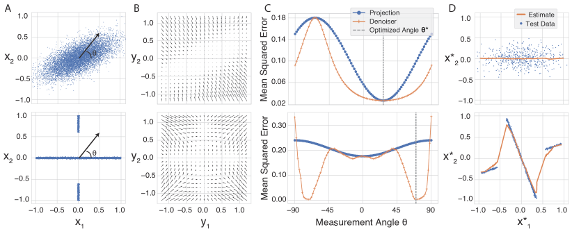
Figure 1: Reconstruction of 2-D signals from a 1-D linear measurement. Top row: Gaussian distribution. Bottom row: K-Sparse distribution. A) Samples from the target distribution (blue points). Measurements are obtained via a dot product of sample and a unit vector (the black vector) parameterized by $\theta$. B) Trained denoiser, $\hat{x}(y)$, depicted as a vector field. Each vector indicates the direction in which the probability of the noisy density increases most rapidly (Eq. 1). C) Mean squared error (MSE) of sample reconstruction as a function of $\theta$, for two estimators: linear projection onto the measurement vector (blue), and reconstruction using the denoiser prior (orange). The dashed vertical line indicates the $\theta^{*}$ obtained with our optimization procedure (based on Equation 8). For sparse prior, our method achieves near-zero error. D) Test data (blue), plotted in a new coordinate system $(x_{1}^{*},x_{2}^{*})$ rotated by $-\theta^{*}$ (i.e., such that the optimal measurement $m$ corresponds to the horizontal coordinate). The bivariate estimates recovered from the optimal linear measurement utilizing the denoiser prior are plotted in orange.

To illustrate our method, we consider two examples of optimal 1-D measurements in a 2-D signal space. In each case, we train a small, two-layer fully-connected denoising network, which is then used to solve the inverse problem via Algorithm 2. As a baseline, we compare this to the reconstruction obtained by linear projection onto the measurement axis. The optimal measurement vector is obtained by evaluating the reconstruction error for a set of densely sampled unit vectors spanning orientations over the range $[-\pi/2,\pi/2]$. The results are illustrated in Figure 1. The top row shows a bivariate Gaussian distribution. In this case, the first PC is the optimal measurement for both reconstruction methods, as expected for a Gaussian prior.

The second row of Figure 1 shows results for the more interesting case of a sparse distribution. In this case, the first PC is aligned with the horizontal which is the optimal measurement vector for linear reconstruction. But the optimal measurement vector for the denoiser prior differs markedly. Furthermore, the reconstruction error at the optimal $\theta^{*}$ is much less than that at $\theta=0$ using linear projection. This improvement arises because the denoiser prior captures the higher-order structure of the data distribution, which is successfully utilized by the nonlinear reconstruction algorithm (see Figure 1D). Importantly, the optimal angle $\theta^{*}$ is correctly identified by our numerical optimization method in all the bivariate cases we have tested (see Supplementary Fig. 1 for an additional example).

3.2 Optimized measurements for MNIST

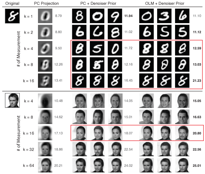
Figure 2: Example image reconstructions using different measurement matrices. Columns show the PC projection, three conditional samples from the denoiser prior using the PCs, and three samples using the OLMs, respectively. Rows correspond to increasing number of measurements, $k$. The numbers indicate the PSNR value of the reconstructions, obtained by averaging over $16$ samples.

We apply our method to find optimal measurement for the MNIST dataset [30]. To learn the prior distribution of these digit images, we train a neural network denoiser. For details of the architecture and training see Appendix E. We apply our method as described in Section 2.4 to obtain the optimized measurement matrix (OLM) for this dataset, for a range of $k$ values.

For comparison, we choose two other types of linear measurements: the top $k$ PCs, and $k$ random vectors, which are the optimal measurements under Gaussian and sparse prior assumptions, respectively. The baseline error is simply that of linear projection onto the span of the PCs. Additionally, using the same $k$ PCs, we compute a non-linear reconstruction based on the denoiser prior. The top half of Figure 2 illustrates our results for a test digit image. First, we observe that combining the PCs with the denoiser prior significantly improves the linear inverse estimates which reflects the power of the denoiser prior. All conditional samples from the denoiser prior appear to be real MNIST images, which then gradually converge to the original as $k$ increases. Optimizing the measurement matrix offers additional improvements in the results, which reflects the importance of the measurements. These improvements are evident in both the identity of the digits and their more detailed appearances (see $k=4$ through $k=16$). Using random measurements (not shown) does not perform as well as either the optimized linear measurements or PCA, on average. See Supplementary Figure 2 for two more examples, including random measurement vectors.

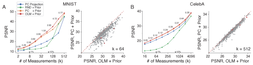
Figure 3: Performance of the optimized linear measurements, for A) MNIST and B) CelebA datasets. Left panel shows the peak signal-to-noise ratio (PSNR) as a function of the number of measurements $k$, for linear reconstruction from PCs (blue), denoiser prior reconstruction from PCs (orange), denoiser prior reconstruction from random measurements (green), and denoiser prior reconstruction from OLMs (red). Numbers indicate increase in PSNR from PC + denoiser prior compare to OLM + prior. The right panel shows a scatter plot comparing the PSNR values using the OLM (x-axis), and PCs (y-axis), over the images in the test set, for a value of $k$ around $10\%$ of the total number of pixels. Red points mark those shown in the examples of Figure 2 and Supplemental Figure 2 and Figure 3.

We quantify our results in terms of peak signal-to-noise ratio (PSNR), as a function of $k$ in the left panel of Figure 3A. The OLMs result in superior reconstruction (red curve), particularly for the values of $k$ ranging from $1\%$ to $30\%$ of the total number of pixels. The peak performance gain from OLM over PC (both utilizing denoiser prior) reached 4.72 dB in PSNR at $k=256$. Additionally, we observe that PC measurements outperform random measurements using the denoiser prior (green), consistent with previous reports obtained with simpler priors [10]. This indicates that the union of subspace priors used in compressed sensing literature does not accurately describe the properties of natural images. Between the two PC reconstructions, the non-linear denoiser prior-based method (orange) shows a considerable improvement over linear reconstruction (blue), demonstrating the large advantage of using the more complex denoiser prior. See Supplemental Table 1 for comparison of our results to other methods in the literature.

In addition to the average performance, we also compare the performance of these methods on individual images in the right panel of Figure 3A, in a scatter plot of the reconstruction errors from measurements using PCs versus that obtained using OLMs. In both cases, nonlinear reconstruction was performed using the denoiser prior; thus the plot highlights the differences due to the linear measurements. Importantly, we observe improvement in performance for almost all images in the test set for the OLM.

3.3 Optimized measurements for CelebA

To test the generality of our method for different image classes, we repeated our experiments on the CelebA dataset [31], which consists of about $200,000$ centered face images. We resized all images to $80\times 80$ and converted them to grayscale. The rest of the procedure is the same as described above. The bottom half of Figure 2 shows an example face image from the test set. Similar to the MNIST case, we observe that using the denoiser prior to reconstruct from PCs significantly improves the linear inverse estimates. Notably, the conditional samples all appear to be realistic face images even for low $k$; this indicates that the denoiser prior adequetly captured the statistical structure of image datasets. As $k$ increases, the reconstructed face images increasingly resemble the originals. Optimizing the measurement matrix offers further improvements in the results, in this case most visible for $k=16$. See Supplementary Figure 3 for two more examples, including reconstructions obtained with random measurements.

The effect of the optimized measurements is investigated quantitatively in Figure 3B. As with the MNIST dataset, we observe that OLM leads to superior reconstruction using the denoiser prior, illustrated by the red curve in the left panel. Note, however, that the improvements in terms of PSNR is smaller than for the MNIST case, although the improvement is noticeable and consistent across all values of $k$. The peak difference in this case is 0.44 dB in PSNR at $k=2048$. Thus, the possible performance gain between PCA and OLM also depends on the specific image dataset. Investigating what aspects of the image statistics drive this difference is of great interest for future study. See also Supplemental Table 1 for comparison of our results to other methods.

Consistent with results on MNIST, for PCs, reconstruction using denoiser prior results in higher performance than linear reconstruction. And all of these methods outperform reconstruction from random measurements. Lastly, we also confirmed that the improvements from the OLM is nearly universal for all images in our test set (Figure 3B, right panel).

3.4 Comparison of measurement subspaces

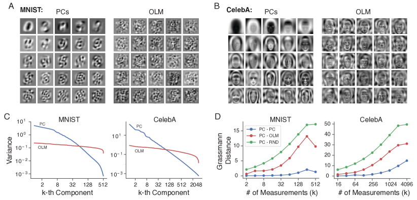
Figure 4: Analysis of optimized measurement vectors. A) Left: Twenty-five selected principal components of the MNIST dataset are visualized as images. They are ordered by variance explained from top to bottom, and left to right. Right: Twenty-five components from the columns of the OLM for $k=64$. B) Same as A) but for the CelebA dataset. C) The variance of the measurement on each component as a function of number of measurements ($k$) for the PCs (blue) and OLMs (red). Note that the optimal measurements are sorted post hoc based on the variance explained by each component. These vectors are optimized jointly for each $k$ and are not ordered by the algorithm itself. D) The Grassmann distance betweensubspaces spanned by different linear measurements as a function of $k$ [32]. We show the distance between subspaces spanned by PCs obtained on two random halves of the training data (blue), between subspaces spanned by PCs and OLM (blue), and between subspaces spanned by PCs and a set of random measurements (green). (see Supplementary Appendix E for a detailed definition of Grassmann distance).

In this section, we present some qualitative and quantitative analyses to help interpret the difference between the linear measurement subspaces defined by PCs and OLMs. For the MNIST dataset, as expected, the first few PCs appear digit-like, and the measurement vectors contain increasing high-spatial frequency content as $k$ increases (Figure 4A, left). The OLMs, on the other hand, do not follow a coarse to fine or a low to fine frequency ordering and appear to have similar patterns (Figure 4A, right). This is reflected, quantitatively, in the exponential decay in measurement variance as a function $k$ for the PCs, while for the OLMs the measurement variance is relatively constant (Figure 4C, left).

Similar phenomena are observed for the CelebA dataset (Figure 4B, C). As expected, the PCs in this case are “eigenfaces” [33]: they contain features that are geometrically aligned with features of the face, with increasing spatial frequency content. The variance of the measurements across PCs fall exponentially. Although the OLMs also have a face-like appearance, they differ from the PCs. Each OLM vector resembles a distorted face with a different identity, giving them an overall template-like appearance. As with the MNIST case, the OLMs all appear to have roughly the same spatial frequency composition. This is consistent with the variances of the measurements, which fall quite slowly across the OLMs (Figure 4C, right).

To quantify the differences between these two sets of measurement vectors, we use the Grassmann distance between the subspaces they span [32, 34]. Figure 4D shows this distance as a function of $k$. As a control, The blue line measures the distance between subspaces arising from PCs computed on two random halves of the training data. As expected, the distance between these two subspaces is small. On the other hand, for both the MNIST and CelebA dataset, the subspaces spanned by the optimal measurements are distinct from those defined by the PCs (Figure 4D, red), but they are more similar to the PCs than to the space defined by a set of random measurements (Figure 4D, green).

3.5 Optimized linear measurements for perceptual loss

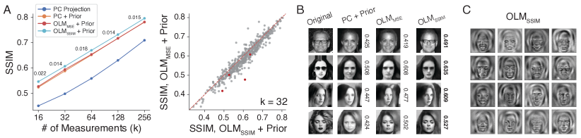
Figure 5: Optimal measurement for perceptual loss (structural similarity index measure - SSIM) [28]. A) Left: SSIM as a function of number of measurement $k$, for PC projection, PC, and OLM optimized for MSE and SSIM, all three using the denoiser prior. The number indicates the increase in SSIM from OLM optimized for MSE to OLM optimized for SSIM. Right: Scatter plot of the SSIM value for individual images, for OLM optimized for SSIM (x-axis) and MSE (y-axis), respectively. B) Example linear inverse solutions obtained from different measurement matrices combined with the denoiser prior. The numbers indicate the SSIM value for each individual image. C) Example measurement vectors from the OLM optimized for SSIM.

The previous sections described measurements optimized for MSE. However, our method is general, and can be used to optimize any differentiable objective function defined on the linear inverse estimates (with the obvious caveat that we cannot guarantee optimality if the function is non-convex).

As an example, we compute a set of OLMs with respect to structural similarity index (SSIM) [28], a commonly-used perceptual image quality metric. Figure 5 shows results obtained using this set of optimal linear measurements. We obtained a noticeable improvement in mean SSIM for a range of $k$, and this improvement applies to the majority of the images in the test set. In Figure 5B, four example images are shown to highlight visually the improvement obtained by optimizing for the SSIM objective. Lastly, in Figure 5C, the SSIM optimized measurement vectors are visualized. These are distinct from both the PCs and MSE optimized vectors shown in Figure 4.

4 Related Work

In this section, we discuss recent developments in specifying natural image priors as well as previous approaches to optimizing linear measurements, including analyses of cameras and biological vision.

Image Priors. Traditionally, prior models have been developed by combining constraints imposed by structural properties, such as translation or dilation invariance, with simple parametric forms, such as Gaussian, mixtures of Gaussian, or local Markov random fields. These models have been used for solving inverse problems with steady and gradual improvement in performance [35, 36, 37, 38, 39, 40, 41, 19]. More recently, methods such as VAEs [42] and GANs [43] have been developed to learn more complex image priors by taking advantage of the increased expressivity of deep neural networks. In the last few years, score-based diffusion models have emerged as the state-of-the-art method for learning sophisticated image priors [44, 45, 46, 47], as evidenced by the high quality of generated images obtained as draws from these priors. Diffusion models rely on the explicit relationship between the MMSE denoising solution and the score of the noisy image density [21, 23, 48]. In addition to enabling unconditional sampling from the implicit prior, the power of that prior can be utilized to obtain high-quality solutions to inverse problems [13, 16, 17]. A closely related line of work known as plug-and-play (P&P) [49] used denoisers as regularizers for solving inverse problems. A number of recent extensions have used this concept to develop MAP solutions for inverse problems [50, 51, 52, 53, 54, 55, 56, 57, 58, 59, 60, 61].

Camera and Sensor Design. The optimal linear measurement problem has arisen in studying the design of cameras or sensory systems. In this case, the sensor measurements are also typically linear, but constrained to be positive-valued and spatially localized. Hardware design considerations often impose additional constraints, for example, that the sensor array must be periodic in its structure. For example, Levin et al. [62] evaluated the impact of different choices in camera design through light field projections in a Bayesian framework. Manning and Brainard [63] enumerated all possible arrangements of a small one-dimensional sensory array to understand the trade-off between spatial and chromatic information, again in the context of a Bayesian framework. Similarly, an important line of work has examined the problem of optimizing the measurements made by retinal circuits using an information-theoretical objective, in some cases combined with biophysical constraints [64, 65, 66, 67, 68, 69]. The recent development of differentiable rendering has also allowed for end-to-end optimization of optical systems [70, 71].

Optimized Linear Measurements. Other work has considered the problem of optimizing linear measurements directly. Weiss et al. [10] observed that neither PCA nor random measurement fully takes into account the statistics of natural images. They attempted to optimize linear measurement using information-based criteria, but were not able to find measurements that outperformed PCA. Wu et al. [72] also proposed a method to find better measurement functions (i.e., both linear and nonlinear) in a compressed sensing framework by using the restricted isometry property [73] as an objective. They showed that the optimized measurement functions (both linear and nonlinear) are superior to simple random measurements, but did not compare their results with PCA. In a different line of work, Burge and Geisler [74] developed a method for finding linear measurements that are optimal for specific downstream tasks, such as estimating the motion presented in a video sequence.

The main advantages of our method are that (1) the linear measurements are optimized directly with respect to the end objective of the reconstruction problem, and that (2) we incorporate a highly expressive learned prior to exploit the higher-order statistics of natural images. As was shown in Section 2, our method outperforms both random measurements and PCA.

5 Conclusion

We present a method for finding optimal linear measurements, using a nonlinear reconstruction method based on a learned prior embedded in a denoiser. We show numerically that the set of linear measurements found through our method, result in superior image reconstruction. This result shows that for signals with non-Gaussian distributions, better measurements exist for minimizing MSE, even though projections onto the PCs maximize the explained variance. The key components of our method are: (i) a denoising diffusion model, which allows us to learn a complex prior underlying the datasets; (ii) a constrained sampling algorithm for obtaining linear inverse estimates from the diffusion prior; and (iii) an end-to-end optimization procedure to find the measurement matrix that minimizes a loss function defined with respect to the linear inverse estimates. We show that the optimal measurement are sensitive to both the statistics of the image dataset, and to the objective function for which they are optimized. Our results highlight the importance of accurately modeling the statistics of the signals to design efficient linear measurements.

One major limitation of our current work is that optimizing linear measurements through the iterative diffusion process is more computationally expensive than PCA and CS. Additionally, the OLMs are obtained separately for each $k$, and are therefore not sequentially ordered like the principal components. Here, we have restricted ourselves to linear measurements to maintain a direct connection to classical signal processing literature, as they are easier to understand and visualize. An interesing directions for future work is to analyze in greater depth the mechanisms through which the measurement subspace specified by OLMs leads to better linear inverse estimates. Additionally, it is of interest to expand the current results to linear measurements with realistic noise models and measurement constraints such as locality and non-negativity. Finally, extending our work to nonlinear measurement functions will be of great interest, representing a form of nonlinear compression problem (e.g., Ballé et al. [75]), with reconstruction through conditional sampling from diffusion models.

Appendix

Appendix A Tweedie / Miyasawa Proof

For completeness, we provide the proof of the core relationship underlying diffusion models [21, 22, 24, 76]. Consider the problem of estimating a natural image $x$ given a noise-corrupted measurement $y=x+\epsilon$, with $\epsilon\sim\mathcal{N}(0,\sigma^{2}I)$. The estimate $\hat{x}(y)$ is chosen to minimize the mean of the squared error $||x-\hat{x}(y)||_{2}^{2}$ over all images $x$ and observations $y$ corrupted with known $\sigma^{2}$. In Bayesian terms, the solution to this denoising problem is the posterior mean:

$$\hat{x}(y)=\int x\ p(x|y)\ dx=\int x\ \frac{p(y|x)p(x)}{\int p(y|x)p(x)dx}\ dx.$$ (10)

Miyasawa [21] showed that the optimal estimator has a direct relationship to the score function of $\nabla\log p(y)$. First, write $p(y)=\int p(y|x)p(x)dx$. Assuming a Gaussian PDF for $p(y|x)$ and taking the gradient with respect to $y$ gives:

$$\nabla_{y}p(y)=\frac{1}{\sigma^{2}}\int(x-y)p(y|x)p(x)dx.$$ (11)

Dividing both sides by $p(y)$ yields:

$$\sigma^{2}\frac{\nabla_{y}p(y)}{p(y)} =\int(x-y)\frac{p(x,y)}{p(y)}dx$$ (12)

$$=\int(x-y)p(x|y)dx$$

$$=\int xp(x|y)dx-\int yp(x|y)dx.$$

Simplifying this gives the result:

$$\sigma^{2}\nabla_{y}\log p(y)=\hat{x}(y)-y.$$ (13)

Thus, the residual of the optimal denoiser, $\hat{x}(y)-y$ is proportional to the gradient of $\log p(y)$. Note that $p(y)$ is equal to the signal prior $p(x)$ convolved with (blurred by) a Gaussian with variance $\sigma^{2}$. This quantity can be used to sample from the implicit prior $p(x)$, for example, by using annealed Langevin dynamics, where the noise $\sigma^{2}$ corresponds to different temperature levels [45, 77, 78]. See Appendix D for a detailed description of our sampling procedure.

Appendix B Principal Components Analysis

Denote by $X$ the data matrix where the columns are individual mean-subtracted samples $x_{i}$. The linear projection is defined as $\hat{x_{i}}=MM^{T}x_{i}$, where $M$ is a matrix with orthogonal columns. Plugging this expression into Equation 5, we have the expected squared-error loss for linear projection:

$$l(M) =\frac{1}{N}\sum_{i}||x_{i}-MM^{T}x_{i}||_{2}^{2}$$ (14)

$$=\frac{1}{N}\ \text{Tr}[(X-MM^{T}X)^{T}(X-MM^{T}X)]$$

$$=\frac{1}{N}\ (\text{Tr}[X^{T}X]-\text{Tr}[M^{T}XX^{T}M])$$

$$=\frac{1}{N}\ (\text{Tr}[X^{T}X]-\sum_{i}[m_{i}^{T}XX^{T}m])$$

To minimize $l(M)$, the $m_{i}$’s should be the eigenvectors associated with the largest eigenvalues of $XX^{T}$, which is the empirical covariance matrix. Note that this solution does not assume a Gaussian data distribution: For any data, the optimal linear projection is the projection onto the leading principal components of the covariance matrix.

When the data is in fact Gaussian distributed, linear projection onto the first $k$ PCs does achieve the minimal error possible, as shown in the bivariate example in Fig. 1A. Otherwise, for non-Gaussian distribution, nonlinear estimation based on the linear measurements can be used to improve performance.

Appendix C Sampling Algorithm

Algorithm 1 Sampling via ascent of the log-likelihood gradient from a denoiser residual

1:denoiser $f$, step size $h$, stochasticity from injected noise $\beta$, initial noise level $\sigma_{0}$, final noise level $\sigma_{\infty}$, distribution mean $m$

2:$t=0$

3:Draw $x_{0}\sim\mathcal{N}(m,\sigma_{0}^{2}\mathrm{Id})$

4:while $\sigma_{t}\geq\sigma_{\infty}$ do

5:     $t\leftarrow t+1$

6:     $s_{t}\leftarrow f(x_{t-1})-x_{t-1}$ $\triangleright$ Compute the score from the denoiser residual

7:     $\sigma_{t}^{2}\leftarrow||s_{t}||^{2}/{d}$ $\triangleright$ Compute the current noise level for stopping criterion

8:     $\gamma_{t}^{2}=\left((1-\beta h)^{2}-(1-h)^{2}\right)\sigma_{t}^{2}$ 

9:     Draw $z_{t}\sim\mathcal{N}(0,I)$ 

10:     $x_{t}\leftarrow x_{t-1}+hd_{t}+\gamma_{t}z_{t}$ $\triangleright$ Perform a partial denoiser step and add noise

11:end while

12:return $x_{t}$

Appendix D Constrained Sampling Algorithm

We adopt a previously developed sampling algorithm for solving linear inverse problems [13]. Given a trained least-squares denoiser $\hat{x}(y)$, define the denoiser residual $g(y)=\hat{x}(y)-y$, which is equal to the score of the learned implicit distribution, $\nabla_{y}\log p(y)$. The orthogonal linear measurement matrix is denoted as $M\in\mathcal{R}^{d\times k}$. The parameters of the algorithm are step size $h$, the magnitude of injected noise $\beta$, and a stopping criterion $\sigma_{end}$. The inputs are the linear measurements $m\in\mathcal{R}^{k}$.

Algorithm 2 Constrained sampling for solving linear inverse problem

1:$m$, $g$, $M$, $h$, $\beta$, $\sigma_{end}$

2:$t\leftarrow 1$ $\triangleright$ initialization

3:$\mu\leftarrow 0.5(\mathbf{1}-MM^{T}\mathbf{1})+Mm$

4:$y_{1}\leftarrow\mathcal{N}(\mu,\ I)$

5:$\sigma^{2}_{1}\leftarrow||g(y_{1})||^{2}_{2}/d$

6:while $\ \sigma_{t}>\sigma_{end}\$ do $l_{t}\leftarrow(I-MM^{T})g(y_{t})+M(m-M^{T}y_{t})$ $\triangleright$ compute the conditional gradient $\gamma^{2}\leftarrow[{(1-\beta*h)^{2}-(1-h)^{2}}]*\sigma^{2}_{t}$ $\triangleright$ scale factor for the added noise $y_{t+1}\leftarrow y_{t}+h*l_{t}+\gamma*\mathcal{N}(0,I)$ $\triangleright$ move up the gradient and add noise $\sigma^{2}_{t+1}\leftarrow||l_{t}||^{2}_{2}/d$ $\triangleright$ compute an estimated noise level $t\leftarrow t+1$

7:end while

For the current paper, we chose $h=0.1$, $\beta=0.1$, and $\sigma_{end}=0.01$.

Appendix E Experimental Details

E.1 Dataset

We used two primary two datasets for our experimental results. The CelebA celebrity faces dataset [31], which contains approximately $200,000$ images, and the MNIST handwritten digits dataset, which contains $60,000$ images [30]. For the CelebA dataset, we downsampled the images to a resolution of $80\times 80\times 1$ grayscale in our main results. The images in the MNIST dataset are the original $28\times 28\times 1$ grayscale.

In both cases, we randomly selected $n=512$ images as the test set. The rest of the images were used for training the denoiser, computing the principal components, and optimizing the linear measurement matrix. The test set was only used for reporting the final performance of the optimized linear measurements.

E.2 CNN denoiser

We performed empirical experiments using UNet architecture. Our UNet networks contain 3 encoder blocks, one mid-level block, and 3 decoder blocks [79]. (For MNIST images we reduced the encoder and decoder blocks to 2, since they are smaller images.) Each block consists of 2 convolutional layers followed by a ReLU non-linearity and bias-free batch-normalization. Each encoder block is followed by a $2\times 2$ spacial down-sampling and a 2 fold increase in the number of channels. Each decoder block is followed by a $2\times 2$ spacial upsampling and a 2 fold reduction of channels. The total number of parameters is $7.6m$. All the denoisers are “bias-free”: we remove all additive constants from convolution and batch-normalization operations (i.e., the batch normalization does not subtract the mean). This facilitates universality (denoisers can operate at all noise levels) see Mohan et al. [80].

We follow the training procedure described in Mohan et al. [80], minimizing the mean squared error in denoising images corrupted by i.i.d. Gaussian noise with standard deviations drawn from the range $[0,1]$ (relative to image intensity range $[0,1]$). Training is carried out on batches of size $512$, for $1000$ epochs. Note that all denoisers are universal and blind: they are trained to handle a range of noise, and the noise level is not provided as input to the denoiser. These properties are exploited by the sampling algorithm, which can operate without manual specification of the step size schedule [13]. This method produces high-quality results in generative sampling, as well as sampling conditioned on linear measurements [15]. To train each denoiser, 4 NVIDIA A100 GPU were used. The total training time for each denoiser was around 10 hours.

E.3 MMSE estimate

We construct the linear inverse estimate by averaging multiple samples obtained using Algorithm 2. The individual samples are shown in Figure 2 and Supplementary Figure 2 and Figure 3. Averaging multiple samples achieves a lower MSE by approximating the posterior mean, which we use when reporting performance (PSNR values). The number of samples $n$ is set to $n=2$ when optimizing the linear measurement to limit memory footprint, and $n=16$ when reporting performance on test data.

E.4 Optimizing linear measurement

We search for the optimal linear measurement by performing stochastic gradient descent in the space of orthogonal matrices as described in the main text. The linear inverse procedure Algorithm 2 is end-to-end differentiable, and thus optimization of the measurement matrix can be done directly in PyTorch by taking derivatives of reconstruction loss with respect to the matrix parameterization. In all cases, we used the Adam optimizer [27] with a learning rate of $10^{-4}$ with exponential decay of $0.90$. We used a batch size of $64$, and training was run for $16$ epochs. The optimization was done on a single node in a GPU cluster, with 4 NVIDIA A100 GPUs. The optimization for a single OLM requires a few hours for the MNIST dataset, and about 24 hours for the CelebA dataset.

E.5 Subspace distance

To quantify the difference between two linear measurement subspaces, we used the distance defined on the Grassmann manifold of subspaces. Concretely, given two linear subspaces $F$ and $G$ defined by the column of two measurement matrices $M_{1}$ and $M_{2}$, the principal angles $\mathbf{\theta}=(\theta_{1},\theta_{2},...,\theta_{k})$ are defined sequentially as [34]:

$$\cos\theta_{k}=\max_{v_{k}\in F}\max_{v_{k}\in G}u^{T}_{k}v_{k},\ \ ||u_{k}||_{2}=1,||v_{k}||_{2}=1$$ (15)

$$\text{subject to}\ \ u^{T}_{k}u_{j}=0,v^{T}_{k}v_{j}=0,\ \forall j=1,2,...,k-1.$$

The principle angles can be computed numerically using the singular value decomposition as described in [81]. The Grassmann distance is defined as the $L_{2}$ norm on the vector of principal angles $\theta$:

$$d_{k}(F,G)=(\sum_{i=1}^{k}\theta_{i}^{2})^{1/2}.$$ (16)

Appendix F Supplementary Figures / Tables

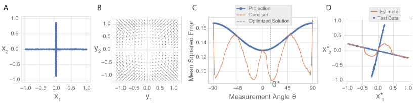
Supplementary Figure 1: Additional example of 1-D linear measurement optimized for a bivariate distribution (sum of two Gaussian ridges) approximating the “union-of-subpaces” prior used in compressed sensing [10]. A) Samples from the target bivariate distribution. B) Residual vector field of the trained denoiser, $\hat{x}(y)-y$. The Miyasawa relationship (Equation 1) states that these vectors indicate the direction in which the log of the noisy density increases most rapidly. C) Estimation error (MSE) as a function of the angle of the 1-D measurement vector. Blue: Estimate obtained by projection onto the measurement vector. Orange: Estimate obtained by computing the conditional mean under the denoiser prior. The dashed gray line marks the measurement angle $\theta^{*}$ found by our optimization procedure. D) Original data from (A) rotated by $-\theta^{*}$, such that the optimal measurement for the new distribution $p(x^{\prime})$ is the value along the horizontal axis ($x^{\prime}_{1}$). The nonlinear bivariate estimates of $x^{\prime}$ are plotted as a function of measurement $m=x^{\prime}_{1}$ (orange line). Note that the nonlinear estimates are obtained by averaging over multiple conditional samples, which can result in deviations from the data distribution. In general, the MMSE solution derived from averaging may exhibit lower visual quality because it can deviate from the (curved) manifold of images.

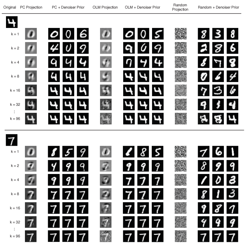
Supplementary Figure 2: Individual samples of the linear inverse estimates from the denoiser prior for two example digit images in the MNIST dataset. The leftmost columns show the PC projection. The next three columns show individual stochastic samples from the denoiser prior, conditioned on the PC measurements. The middle set of columns show the OLM projection, and the samples conditioned on the OLMs. The last set of columns show the results from a random measurement matrix. Rows correspond to increasing number of measurement $k$.

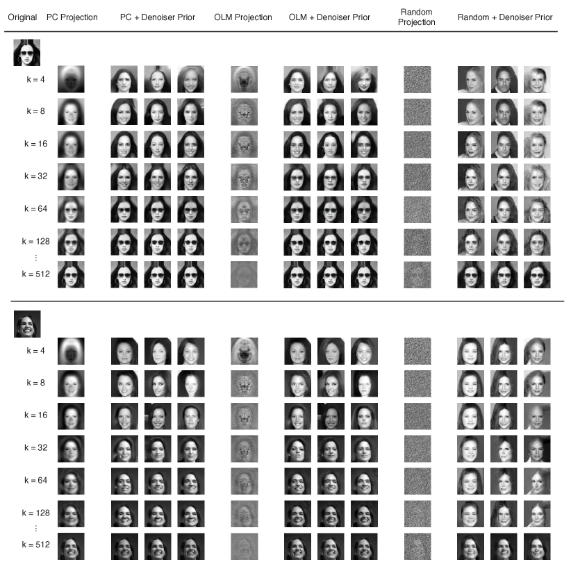
Supplementary Figure 3: Individual samples of the linear inverse estimates from the denoiser prior for two example digit images in the CelebA dataset. The leftmost columns show the PC projection. The next three columns show individual stochastic samples from the denoiser prior, conditioned on the PC measurements. The middle set of columns show the OLM projection, and the samples conditioned on the OLMs. The last set of columns show the results from a random measurement matrix. Rows correspond to increasing number of measurement $k$.

	METHODS	Bora et al. [12]		Wu et al. [72]		Our Method
DATASET		LASSO (Wavelet)	VAE or GAN Prior	Learned Linear*	Learned Non-Linear*	PC + Prior	OLM + Prior*
MNIST, k = 25		103	17.2	4.0 ± 1.4	3.4 ± 1.2	4.31 ± 0.13	3.47 ± 0.11
MNIST, k = 50		86	8.9	/	/	1.59 ± 0.05	1.20 ± 0.03
MNIST, k = 250		49.1	6.2	/	/	0.13 ± 0.01	0.04 ± 0.002
CelebA, k = 50		$\sim$ 235	$\sim$ 129	$\sim$ 32.0 ± 6.7	$\sim$ 28.9 ± 6.7	39.31 ± 0.86	38.29 ± 0.84
CelebA, k = 100		$\sim$ 197	$\sim$ 76	/	/	25.51 ± 0.61	24.77 ± 0.58
CelebA, k = 500		$\sim$ 102	$\sim$ 36	/	/	9.75 ± 0.27	9.01 ± 0.26

Table 1: Compare reconstruction performance to different compressed sensing methods. We compare the per-image MSE (lower is better) of our method with previous methods for compressed sensing using deep neural networks [12, 72]. Methods with symbol “*” use measurement function that are explicitly optimized; The symbol “/ ” indicates the results are not available, as Wu et al. [72] reported performance only for small $k$; The symbol “$\sim$” indicates the MSE are estimated from images of different size (64 x 64) assuming a constant per-pixel error. In addition, $\pm$ indicates standard error of the mean. Bold numbers highlight the best result for linear measurement.

We compare the per-image MSE of our method with previously proposed methods for compressed sensing using deep neural networks [12, 72]. Bora et al. [12] used both VAE and GAN as image priors to obtain the linear inverse solution. Their methods outperform standard method for compressed sensing using LASSO (sparse prior) in the wavelet domain. They did not attempt to optimize the measurement matrix, and as a result were vastly outperformed by our method.

Wu et al. [72] optimized both linear and nonlinear measurements using the restricted isometry property as an objective, but only for very small $k$. We found that on MNIST, our OLM is able to match the performance of even the nonlinear measurement function. On CelebA dataset, for $k=50$, we obtained slightly worse performance for the OLMs compared to the learned linear measurements in Wu et al. [72]. However, we may have underestimated the error in Wu et al. [72], as we estimated MSE based on images of a smaller size (64 x 64) from their results but assumed a constant per-pixel error. Furthermore, our method is most effective for $k$ at around $10\%$ of the total number of pixels. Thus, we expect our advantage to improve further for larger $k$. Lastly, our method has the distinct feature that we can produce individual high-probability samples, in addition to the MMSE solution.

References

- Ribes and Schmitt [2008] Alejandro Ribes and Francis Schmitt. Linear inverse problems in imaging. IEEE Signal Processing Magazine, 25(4):84–99, 2008.
- Yue et al. [2016] Linwei Yue, Huanfeng Shen, Jie Li, Qiangqiang Yuan, Hongyan Zhang, and Liangpei Zhang. Image super-resolution: The techniques, applications, and future. Signal processing, 128:389–408, 2016.
- Bertalmio et al. [2000] Marcelo Bertalmio, Guillermo Sapiro, Vincent Caselles, and Coloma Ballester. Image inpainting. In Proceedings of the 27th annual conference on Computer graphics and interactive techniques, pages 417–424, 2000.
- Tao et al. [2018] Xin Tao, Hongyun Gao, Xiaoyong Shen, Jue Wang, and Jiaya Jia. Scale-recurrent network for deep image deblurring. In Proceedings of the IEEE conference on computer vision and pattern recognition, pages 8174–8182, 2018.
- Zhang et al. [2016] Richard Zhang, Phillip Isola, and Alexei A Efros. Colorful image colorization. In Computer Vision–ECCV 2016: 14th European Conference, Amsterdam, The Netherlands, October 11-14, 2016, Proceedings, Part III 14, pages 649–666. Springer, 2016.
- Donoho [2006] David L Donoho. Compressed sensing. IEEE Transactions on information theory, 52(4):1289–1306, 2006.
- Tropp [2006] Joel A Tropp. Just relax: Convex programming methods for identifying sparse signals in noise. IEEE transactions on information theory, 52(3):1030–1051, 2006.
- Portilla et al. [2003a] J. Portilla, V. Strela, M.J. Wainwright, and E.P. Simoncelli. Image denoising using scale mixtures of gaussians in the wavelet domain. IEEE Transactions on Image Processing, 12(11):1338–1351, 2003a. doi: 10.1109/TIP.2003.818640.
- Ballé et al. [2016] J Ballé, V Laparra, and E P Simoncelli. Density modeling of images using a generalized normalization transformation. In Int’l Conf on Learning Representations (ICLR), San Juan, Puerto Rico, May 2016. URL http://arxiv.org/abs/1511.06281.
- Weiss et al. [2007] Yair Weiss, Hyun Sung Chang, and William T Freeman. Learning compressed sensing. In Snowbird Learning Workshop, Allerton, CA, 2007.
- Romano et al. [2017a] Yaniv Romano, Michael Elad, and Peyman Milanfar. The little engine that could: Regularization by denoising (red). SIAM Journal on Imaging Sciences, 10(4):1804–1844, 2017a.
- Bora et al. [2017] Ashish Bora, Ajil Jalal, Eric Price, and Alexandros G Dimakis. Compressed sensing using generative models. In International conference on machine learning, pages 537–546. PMLR, 2017.
- Kadkhodaie and Simoncelli [2020] Zahra Kadkhodaie and Eero P Simoncelli. Solving linear inverse problems using the prior implicit in a denoiser. arXiv preprint arXiv:2007.13640, 2020.
- Song et al. [2021] Yang Song, Liyue Shen, Lei Xing, and Stefano Ermon. Solving inverse problems in medical imaging with score-based generative models. arXiv preprint arXiv:2111.08005, 2021.
- Kadkhodaie and Simoncelli [2021] Zahra Kadkhodaie and Eero Simoncelli. Stochastic solutions for linear inverse problems using the prior implicit in a denoiser. Advances in Neural Information Processing Systems, 34:13242–13254, 2021.
- Kawar et al. [2022] Bahjat Kawar, Michael Elad, Stefano Ermon, and Jiaming Song. Denoising diffusion restoration models. Advances in Neural Information Processing Systems, 35:23593–23606, 2022.
- Chung et al. [2022] Hyungjin Chung, Byeongsu Sim, Dohoon Ryu, and Jong Chul Ye. Improving diffusion models for inverse problems using manifold constraints. Advances in Neural Information Processing Systems, 35:25683–25696, 2022.
- Geman and Geman [1984] Stuart Geman and Donald Geman. Stochastic relaxation, gibbs distributions, and the bayesian restoration of images. IEEE Transactions on pattern analysis and machine intelligence, pages 721–741, 1984.
- Lyu and Simoncelli [2008] Siwei Lyu and Eero P Simoncelli. Modeling multiscale subbands of photographic images with fields of gaussian scale mixtures. IEEE Transactions on pattern analysis and machine intelligence, 31(4):693–706, 2008.
- Zoran and Weiss [2011] D Zoran and Y Weiss. From learning models of natural image patches to whole image restoration. In IEEE International Conference for Computer Vision, 2011.
- Miyasawa [1961] Koichi Miyasawa. An empirical bayes estimator of the mean of a normal population. Bull. Inst. Internat. Statist, 38(181-188):1–2, 1961.
- Robbins [1992] Herbert E Robbins. An empirical bayes approach to statistics. In Breakthroughs in Statistics: Foundations and basic theory, pages 388–394. Springer, 1992.
- Raphan and Simoncelli [2011] M Raphan and E P Simoncelli. Least squares estimation without priors or supervision. Neural Computation, 23(2):374–420, Feb 2011. doi: 10.1162/NECO_a_00076.
- Efron [2011] Bradley Efron. Tweedie’s formula and selection bias. Journal of the American Statistical Association, 106(496):1602–1614, 2011.
- Trefethen and Bau [2022] Lloyd N Trefethen and David Bau. Numerical linear algebra, volume 181. SIAM, 2022.
- Shepard et al. [2015] Ron Shepard, Scott R Brozell, and Gergely Gidofalvi. The representation and parametrization of orthogonal matrices. The Journal of Physical Chemistry A, 119(28):7924–7939, 2015.
- Kingma and Ba [2014] Diederik P Kingma and Jimmy Ba. Adam: A method for stochastic optimization. arXiv preprint arXiv:1412.6980, 2014.
- Wang et al. [2004] Zhou Wang, Alan C Bovik, Hamid R Sheikh, and Eero P Simoncelli. Image quality assessment: from error visibility to structural similarity. IEEE transactions on image processing, 13(4):600–612, 2004.
- Detlefsen et al. [2022] Nicki Skafte Detlefsen, Jiri Borovec, Justus Schock, Ananya Harsh Jha, Teddy Koker, Luca Di Liello, Daniel Stancl, Changsheng Quan, Maxim Grechkin, and William Falcon. Torchmetrics-measuring reproducibility in pytorch. Journal of Open Source Software, 7(70):4101, 2022.
- Deng [2012] Li Deng. The mnist database of handwritten digit images for machine learning research [best of the web]. IEEE signal processing magazine, 29(6):141–142, 2012.
- Liu et al. [2015] Ziwei Liu, Ping Luo, Xiaogang Wang, and Xiaoou Tang. Deep learning face attributes in the wild. In Proceedings of International Conference on Computer Vision (ICCV), 2015.
- Hamm and Lee [2008] Jihun Hamm and Daniel D Lee. Grassmann discriminant analysis: a unifying view on subspace-based learning. In Proceedings of the 25th international conference on Machine learning, pages 376–383, 2008.
- Turk and Pentland [1991] Matthew Turk and Alex Pentland. Eigenfaces for recognition. Journal of cognitive neuroscience, 3(1):71–86, 1991.
- Björck and Golub [1973] Ake Björck and Gene H Golub. Numerical methods for computing angles between linear subspaces. Mathematics of computation, 27(123):579–594, 1973.
- Donoho [1995] D Donoho. Denoising by soft-thresholding. IEEE Trans Info Theory, 43:613–627, 1995.
- Simoncelli and Adelson [1996] Eero P Simoncelli and Edward H Adelson. Noise removal via bayesian wavelet coring. In Proceedings of 3rd IEEE International Conference on Image Processing, volume 1, pages 379–382. IEEE, 1996.
- Moulin and Liu [1999] P Moulin and J Liu. Analysis of multiresolution image denoising schemes using a generalized Gaussian and complexity priors. IEEE Trans Info Theory, 45:909–919, 1999.
- Hyvärinen [1999] Hyvärinen. Sparse code shrinkage: Denoising of nonGaussian data by maximum likelihood estimation. Neural Computation, 11(7):1739–1768, 1999.
- Romberg et al. [2001] J. Romberg, H. Choi, and R. Baraniuk. Bayesian tree-structured image modeling using wavelet-domain hidden Markov models. IEEE Trans Image Proc, 10(7), July 2001.
- Şendur and Selesnick [2002] L Şendur and I W Selesnick. Bivariate shrinkage functions for wavelet-based denoising exploiting interscale dependency. IEEE Trans Signal Proc, 50(11):2744–2756, November 2002.
- Portilla et al. [2003b] J Portilla, V Strela, M J Wainwright, and E P Simoncelli. Image denoising using scale mixtures of Gaussians in the wavelet domain. IEEE Trans Image Proc, 12(11):1338–1351, Nov 2003b. doi: 10.1109/TIP.2003.818640.
- Kingma and Welling [2013] Diederik P Kingma and Max Welling. Auto-encoding variational bayes. arXiv preprint arXiv:1312.6114, 2013.
- Goodfellow et al. [2020] Ian Goodfellow, Jean Pouget-Abadie, Mehdi Mirza, Bing Xu, David Warde-Farley, Sherjil Ozair, Aaron Courville, and Yoshua Bengio. Generative adversarial networks. Communications of the ACM, 63(11):139–144, 2020.
- Sohl-Dickstein et al. [2015] Jascha Sohl-Dickstein, Eric Weiss, Niru Maheswaranathan, and Surya Ganguli. Deep unsupervised learning using nonequilibrium thermodynamics. In International conference on machine learning, pages 2256–2265. PMLR, 2015.
- Song and Ermon [2019] Yang Song and Stefano Ermon. Generative modeling by estimating gradients of the data distribution. Advances in neural information processing systems, 32, 2019.
- Ho et al. [2020] Jonathan Ho, Ajay Jain, and Pieter Abbeel. Denoising diffusion probabilistic models. Advances in neural information processing systems, 33:6840–6851, 2020.
- Nichol and Dhariwal [2021] Alex Nichol and Prafulla Dhariwal. Improved denoising diffusion probabilistic models. Int’l Conf Machine Learning, 38, 2021.
- Vincent [2011] Pascal Vincent. A connection between score matching and denoising autoencoders. Neural Computation, 23(7):1661–1674, 2011. doi: 10.1162/NECO\_a\_00142.
- Venkatakrishnan et al. [2013] Singanallur V Venkatakrishnan, Charles A Bouman, and Brendt Wohlberg. Plug-and-play priors for model based reconstruction. In 2013 IEEE Global Conference on Signal and Information Processing, pages 945–948. IEEE, 2013.
- Chan et al. [2016] Stanley H Chan, Xiran Wang, and Omar A Elgendy. Plug-and-play admm for image restoration: Fixed-point convergence and applications. IEEE Transactions on Computational Imaging, 3(1):84–98, 2016.
- Romano et al. [2017b] Yaniv Romano, Michael Elad, and Peyman Milanfar. The little engine that could: Regularization by denoising (RED). CoRR, abs/1611.02862, 2017b. URL http://arxiv.org/abs/1611.02862.
- Zhang et al. [2017] Kai Zhang, Wangmeng Zuo, Shuhang Gu, and Lei Zhang. Learning deep cnn denoiser prior for image restoration. In Proc. IEEE Conf. on Computer Vision and Pattern Recognition (CVPR), volume 2, 2017.
- Kamilov et al. [2017] Ulugbek S Kamilov, Hassan Mansour, and Brendt Wohlberg. A plug-and-play priors approach for solving nonlinear imaging inverse problems. IEEE Signal Processing Letters, 24(12):1872–1876, 2017.
- Meinhardt et al. [2017] T. Meinhardt, M. Moeller, C. Hazirbas, and D. Cremers. Learning proximal operators: Using denoising networks for regularizing inverse imaging problems. In 2017 IEEE International Conference on Computer Vision (ICCV), pages 1799–1808, 2017. doi: 10.1109/ICCV.2017.198.
- Chan et al. [2017] S. H. Chan, X. Wang, and O. A. Elgendy. Plug-and-play admm for image restoration: Fixed-point convergence and applications. IEEE Transactions on Computational Imaging, 3(1):84–98, 2017. doi: 10.1109/TCI.2016.2629286.
- Mataev et al. [2019] Gary Mataev, Peyman Milanfar, and Michael Elad. Deepred: Deep image prior powered by red. In Proceedings of the IEEE International Conference on Computer Vision Workshops, pages 0–0, 2019.
- Teodoro et al. [2019] Afonso M Teodoro, José M Bioucas-Dias, and Mário AT Figueiredo. Image restoration and reconstruction using targeted plug-and-play priors. IEEE Transactions on Computational Imaging, 5(4):675–686, 2019.
- Sun et al. [2019] Y. Sun, B. Wohlberg, and U. S. Kamilov. An online plug-and-play algorithm for regularized image reconstruction. IEEE Transactions on Computational Imaging, 5(3):395–408, 2019. doi: 10.1109/TCI.2019.2893568.
- Reehorst and Schniter [2019] E. T. Reehorst and P. Schniter. Regularization by denoising: Clarifications and new interpretations. IEEE Transactions on Computational Imaging, 5(1):52–67, 2019. doi: 10.1109/TCI.2018.2880326.
- Pang et al. [2020] Tongyao Pang, Yuhui Quan, and Hui Ji. Self-supervised bayesian deep learning for image recovery with applications to compressive sensing. In Computer Vision–ECCV 2020: 16th European Conference, Glasgow, UK, August 23–28, 2020, Proceedings, Part XI 16, pages 475–491. Springer, 2020.
- Sun et al. [2023] Yu Sun, Zihui Wu, Yifan Chen, Berthy T Feng, and Katherine L Bouman. Provable probabilistic imaging using score-based generative priors. arXiv preprint arXiv:2310.10835, 2023.
- Levin et al. [2008] Anat Levin, William T Freeman, and Frédo Durand. Understanding camera trade-offs through a bayesian analysis of light field projections. In Computer Vision–ECCV 2008: 10th European Conference on Computer Vision, Marseille, France, October 12-18, 2008, Proceedings, Part IV 10, pages 88–101. Springer, 2008.
- Manning and Brainard [2009] Jeremy R Manning and David H Brainard. Optimal design of photoreceptor mosaics: why we do not see color at night. Visual neuroscience, 26(1):5–19, 2009.
- Atick and Redlich [1992] Joseph J Atick and A Norman Redlich. What does the retina know about natural scenes? Neural computation, 4(2):196–210, 1992.
- Karklin and Simoncelli [2011] Yan Karklin and Eero Simoncelli. Efficient coding of natural images with a population of noisy linear-nonlinear neurons. Advances in neural information processing systems, 24, 2011.
- Jun et al. [2021] Na Young Jun, Greg D Field, and John Pearson. Scene statistics and noise determine the relative arrangement of receptive field mosaics. Proceedings of the National Academy of Sciences, 118(39):e2105115118, 2021.
- Roy et al. [2021] Suva Roy, Na Young Jun, Emily L Davis, John Pearson, and Greg D Field. Inter-mosaic coordination of retinal receptive fields. Nature, 592(7854):409–413, 2021.
- Jun et al. [2022] Na Young Jun, Greg Field, and John Pearson. Efficient coding, channel capacity, and the emergence of retinal mosaics. Advances in neural information processing systems, 35:32311–32324, 2022.
- Zhang et al. [2022] Ling-Qi Zhang, Nicolas P Cottaris, and David H Brainard. An image reconstruction framework for characterizing initial visual encoding. Elife, 11:e71132, 2022.
- Tseng et al. [2021] Ethan Tseng, Ali Mosleh, Fahim Mannan, Karl St-Arnaud, Avinash Sharma, Yifan Peng, Alexander Braun, Derek Nowrouzezahrai, Jean-Francois Lalonde, and Felix Heide. Differentiable compound optics and processing pipeline optimization for end-to-end camera design. ACM Transactions on Graphics (TOG), 40(2):1–19, 2021.
- Deb et al. [2022] Diptodip Deb, Zhenfei Jiao, Ruth Sims, Alex Chen, Michael Broxton, Misha B Ahrens, Kaspar Podgorski, and Srinivas C Turaga. Fouriernets enable the design of highly non-local optical encoders for computational imaging. Advances in Neural Information Processing Systems, 35:25224–25236, 2022.
- Wu et al. [2019] Yan Wu, Mihaela Rosca, and Timothy Lillicrap. Deep compressed sensing. In International Conference on Machine Learning, pages 6850–6860. PMLR, 2019.
- Candes [2008] Emmanuel J Candes. The restricted isometry property and its implications for compressed sensing. Comptes rendus. Mathematique, 346(9-10):589–592, 2008.
- Burge and Geisler [2015] Johannes Burge and Wilson S Geisler. Optimal speed estimation in natural image movies predicts human performance. Nature communications, 6(1):7900, 2015.
- Ballé et al. [2016] Johannes Ballé, Valero Laparra, and Eero P Simoncelli. End-to-end optimized image compression. arXiv preprint arXiv:1611.01704, 2016.
- Raphan and Simoncelli [2007] M Raphan and E P Simoncelli. Learning to be Bayesian without supervision. In B Schölkopf, J Platt, and T Hofmann, editors, Adv. Neural Information Processing Systems (NIPS*06), volume 19, pages 1145–1152, Cambridge, MA, May 2007. MIT Press.
- Bussi and Parrinello [2007] Giovanni Bussi and Michele Parrinello. Accurate sampling using langevin dynamics. Physical Review E, 75(5):056707, 2007.
- Bhattacharya and Waymire [2009] Rabi N Bhattacharya and Edward C Waymire. Stochastic processes with applications. SIAM, 2009.
- Ronneberger et al. [2015] Olaf Ronneberger, Philipp Fischer, and Thomas Brox. U-net: Convolutional networks for biomedical image segmentation. In Medical image computing and computer-assisted intervention–MICCAI 2015: 18th international conference, Munich, Germany, October 5-9, 2015, proceedings, part III 18, pages 234–241. Springer, 2015.
- Mohan et al. [2019] Sreyas Mohan, Zahra Kadkhodaie, Eero P Simoncelli, and Carlos Fernandez-Granda. Robust and interpretable blind image denoising via bias-free convolutional neural networks. arXiv preprint arXiv:1906.05478, 2019.
- Knyazev and Argentati [2002] Andrew V Knyazev and Merico E Argentati. Principal angles between subspaces in an a-based scalar product: algorithms and perturbation estimates. SIAM Journal on Scientific Computing, 23(6):2008–2040, 2002.