WeatherFormer: A Pretrained Encoder Model for Learning Robust Weather Representations from Small Datasets

Abstract

This paper introduces WeatherFormer, a transformer encoder-based model designed to learn robust weather features from minimal observations. It addresses the challenge of modeling complex weather dynamics from small datasets, a bottleneck for many prediction tasks in agriculture, epidemiology, and climate science. WeatherFormer was pretrained on a large pretraining dataset comprised of 39 years of satellite measurements across the Americas. With a novel pretraining task and fine-tuning, WeatherFormer achieves state-of-the-art performance in county-level soybean yield prediction and influenza forecasting. Technical innovations include a unique spatiotemporal encoding that captures geographical, annual, and seasonal variations, adapting the transformer architecture to continuous weather data, and a pretraining strategy to learn representations that are robust to missing weather features. This paper for the first time demonstrates the effectiveness of pretraining large transformer encoder models for weather-dependent applications across multiple domains.

1 Introduction

Understanding dynamic weather patterns is extremely important in several major fields including agriculture, epidemiology, climate science, disaster response, and transportation. However, real-world datasets in these fields are small and lack detailed weather measurements. For instance, a crop yield prediction dataset typically contains only 5-7 years of detailed weather data for a few farms (McFarland et al., 2020) or just a few weather measurements over a long period (Khaki et al., 2020). Consequently, large models with sufficient capacity to learn weather patterns overfit when trained on these datasets. On the other hand, without a good representation of weather, any model’s performance for prediction tasks in these fields will remain sub-optimal.

In Natural Language Processing (NLP), the problem of small datasets is tackled by training a large model on a massive unlabelled text dataset, such as the English Wikipedia (Devlin et al., 2019), and then finetuned on small datasets for prediction tasks. This approach with pretrained large models like BERT (Devlin et al., 2019), RoBERTa (Liu et al., 2019b), and others (Clark et al., 2020; Lan et al., 2020) has demonstrated remarkable success in improving the benchmarks on sentiment analysis (Batra et al., 2021), machine translation (Zhu et al., 2020), and reading comprehension (Fernandez et al., 2023).

Unlike text, which is a discrete domain, weather data is continuous and has both spatial and temporal dependencies. Hence, it is unclear if large models pretrained on public weather datasets will improve the performance of the downstream tasks. While recent works such as Man et al. (2023) and Nguyen et al. (2023) have proposed decoder-based (Vaswani et al., 2017) transformer models for weather forecasting and downsampling, no foundational weather model to our knowledge has been trained to extract good representations of weather from a small number of observations.

In this paper, we aim to fill this knowledge gap by pretraining a weather encoder model, called WeatherFormer on a large dataset of satellite-based weather measurements from the NASA Power Project (NASA, 2024). Our model is trained to extract good representations of weather from a small dataset and just a few basic measurements such as the mean temperature and precipitation. It supports a maximum sequence length of 365, allowing it to process up to 1 year of daily weather data, 7 years of weekly weather data, and 30 years of monthly weather data. It also incorporates a new positional encoding mechanism sensitive to geographical location, year, and seasonality, thus enabling it to capture weather patterns’ dynamic and cyclic nature across different times and places. We also observed that Masked Language Modeling (MLM) (Devlin et al., 2019), a common pretraining strategy for encoder models, is suboptimal for pretraining large models with continuous weather data. For a remedy, we propose a novel pretraining strategy to address this shortcoming.

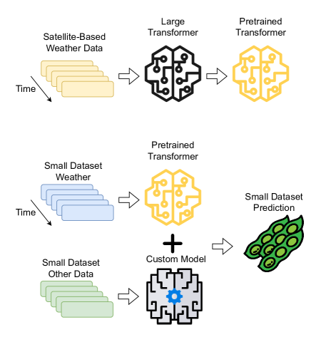
Figure 1: A large transformer model (WeatherFormer) is pretrained on a massive satellite-based weather dataset, enabling the model to learn rich representations of weather during pretraining. This pretrained model can extract robust weather features for a new prediction task (Small Dataset). Even when only a limited number of weather measurements are available for a specific task, the learned weather features can be used to improve the prediction accuracy.

The potential impact of a pretrained encoder weather model such as WeatherFormer is substantial across various domains, including agriculture, epidemiology, climate science, and transportation. Our experiments demonstrate that fine-tuning this model for soybean yield prediction and influenza forecasting in New York City achieves state-of-the-art performance in both tasks. However, the applications extend far beyond these examples. In agriculture, additional applications could be predictions for crop yield, plant diseases, and flowering periods, which are crucial for resource-efficient farming. In epidemiology, the outbreaks of weather-dependent diseases besides influenza, such as dengue (Abdullah et al., 2022), malaria (Hoshen and Morse, 2004), cholera (Christaki et al., 2020), and typhoid (Jia et al., 2024), can be predicted. In climate science, WeatherFormer can be utilized to study various environmental phenomena such as droughts (Balting et al., 2021), coastal flooding (Kirezci et al., 2020), and soil erosion (Eekhout and de Vente, 2022).

Our contributions can be summarized as follows:

• Collected, processed and created a 60 GB dataset of satellite weather measurements ready for training large deep learning models.

• Modified the transformer encoder model with a novel positional encoding, scalers, and a novel pretraining task to pretrain on a large volume of continuous weather data.

• Trained and open-sourced two foundational models for weather, called WeatherFormer, with 2 million and 8 million parameters, respectively.

• Finetuned WeatherFormer models to achieve SOTA performance in Soybeans yield prediction in the US corn belt and Influenza forecasting in New York City.

2 Background and Related Work

2.1 Foundational Models in Deep Learning

Foundational models, exemplified by GPT (Radford et al., 2018) and BERT (Devlin et al., 2019), mark a transformative shift in the development and deployment of deep learning systems in Natural Language Processing (NLP). These models are pre-trained on extensive data corpora and demonstrate an exceptional capacity to generalize across diverse tasks without task-specific training.

The foundational models have also found applications beyond NLP. In meteorology, foundational models have been introduced for short and medium-term weather prediction, downsampling, and climate-related text analysis. Pathak et al. (2022) developed a time series-based recurrent neural network (Hochreiter and Schmidhuber, 1997) for short to medium-range weather forecasting. Lam et al. (2023) employed Graph Neural Networks (Scarselli et al., 2009) to process satellite imaging data for global medium-range weather predictions. More recently, transformer-based models have been deployed for weather forecasting (Man et al., 2023; Nguyen et al., 2023) and data downsampling (Nguyen et al., 2023). Lastly, researchers have developed both encoder-based (Webersinke et al., 2022; Fard et al., 2022) and decoder-based models (Bi et al., 2024) for analyzing climate-related textual data. To the best of our knowledge, no foundational weather model besides WeatherFormer has been trained to extract weather representations for downstream prediction tasks.

2.2 Self-Supervised Learning

Self-Supervised Learning (SSL) trains foundational models on unlabeled datasets using specialized tasks that do not require explicit labels, allowing models to autonomously extract useful information from the data.

Masked Language Modeling (MLM): Introduced by BERT, MLM involves masking certain tokens in a sentence and tasking the model with predicting these tokens using the visible context. The loss function for MLM is formulated as:

$$\mathcal{L}=-\log P(\mathcal{M}|\mathcal{V},\Theta)$$

where $\mathcal{M}$ denotes the masked tokens and $\mathcal{V}$ the visible tokens.

Autoregressive Language Modeling: Popularized by GPT Brown et al. (2020), this approach predicts the next token in a sequence based on the previous tokens, training the model to understand the probability distribution of a language. It is defined mathematically as:

$$\mathcal{L}=-\sum_{k>1}^{n}\log P(x_{k}|x_{1},\dots,x_{k-1},\Theta)$$

Where $x_{1},\dots,x_{k-1}$ are previously generated tokens. This technique has also proven effective for modeling continuous weather data (Nguyen et al., 2023).

Other notable SSL tasks include Replaced Token Detection (Clark et al., 2020) and Next Sentence Prediction (Devlin et al., 2019).

2.3 Machine Learning-based Yield Prediction

Researchers have applied various machine learning methods to predict crop yields from wheat to potatoes using data ranging from on-field measurements to satellite imagery. Farm-level data contains detailed features such as weather conditions, soil characteristics, fertilization, and irrigation, enabling accurate yield predictions (Ruß and Kruse, 2010; Ahamed et al., 2015). In contrast, satellite data lacks such granularity and is generally used for broader yield predictions at regional, state, and national levels (Khaki et al., 2020).

Key algorithms in this domain include neural networks (Ruß et al., 2008; Khaki et al., 2020), regression models (Ruß and Kruse, 2010), random forests (Jeong et al., 2016), and clustering algorithms (Ahamed et al., 2015).

2.4 Influenza Forecasting

Influenza viruses cause significant annual epidemics worldwide, with the 2023-2024 season alone resulting in over 380,000 hospitalizations and 24,000 deaths (CDC, 2024). To combat this, researchers have developed forecasting models that can be categorized into two main types: parametric machine learning-based models and neural network-based models.

Parametric models employ statistical learning techniques to fit epidemiological data for influenza epidemics. Examples include Gaussian Process regression (Zimmer and Yaesoubi, 2020), Dynamic Bayesian models (Osthus et al., 2019), and the Dante system (Osthus and Moran, 2021). Random forest algorithms have also been applied for influenza activity prediction in Eastern China’s subtropical zones (Liu et al., 2019a).

Neural network-based models, particularly those leveraging recurrent neural networks, are used for capturing temporal and spatial dependencies in epidemic data. These models have been successful in predicting weekly influenza trends globally and in the U.S. (Wu et al., 2021; Amendolara et al., 2023). Additionally, recurrent networks have been utilized in China using climate, demography, and search engine data for forecasting influenza-like illnesses (Yang et al., 2023).

3 Data Collection

3.1 Pretraining Dataset

Our pretraining data was downloaded from the NASA Power API (NASA, 2024). We downloaded 28 daily weather measurements from 1984 till 2022. Although the Power API has kept records of weather since 1980, we have found that the earlier years were missing many of the important weather measurements and we chose to exclude them. The dataset consisted of rectangular regions of shape $5^{\circ}\times 8^{\circ}$ spanning the continental United States, Central America, and South America as shown in Figure 7. The dataset contained 119 rectangles, each containing 160 unique coordinates with weather measurements. The spatial resolution of the dataset was $0.5$ degree². Additionally, we computed weekly and monthly averages and concatenated with the dataset. In total, the pretraining dataset contains approximately 9.1 billion floating point numbers.

A detailed description of the dataset is given in section 9.

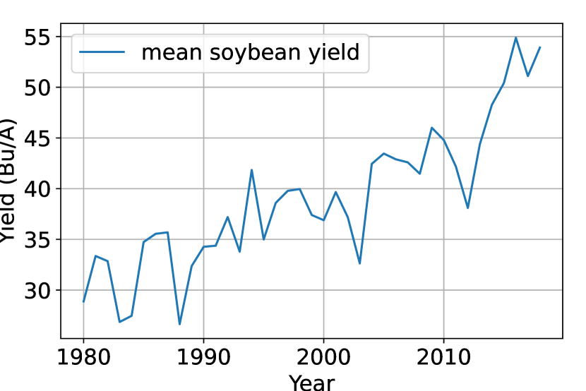
(a) Mean soybean yield (Bu/A) across 9 corn belt counties of the United States.

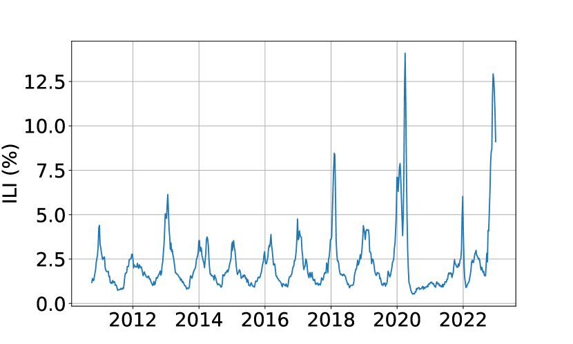
(b) Influenza Like Illness ($\%$) for New York City from 2010 to 2022.

Figure 2: County-level soybean yield and Influenza forecasting for New York City were used as the finetuning tasks for WeatherFormer. The mean soybean yield gradually increased due to hybrid vigor and better farming practices. On the other hand, the influenza seasons show clear peaks during the winter until 2019 and after that, the patterns became irregular due to COVID-19.

3.2 Finetuing Datasets

To evaluate the downstream task performance of WeatherFormer, we predicted soybean yield in the corn belt region of the United States from 1980 to 2022 and also Influenza cases in New York City from 2010 to 2020. Following the conventions from the previous research, we reported Root Mean Square Error in Bu/Acre for the soybeans dataset and Mean Absolute Error (MAE) for the influenza dataset. A detailed description of the fine-tuning datasets, preprocessing, and prediction tasks can be found in section 9.

4 Architecture

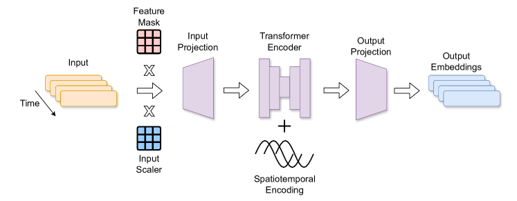
Figure 3: The forward pass of the weather inputs through the WeatherFormer architecture. The input is first multiplied with learnable input scalers and a feature mask and then projected to a hidden dimension through a linear layer. After that, the input goes through a transformer encoder with a novel spatiotemporal encoding mechanism and finally, the input is projected to an output dimension.

In this section, we describe the architecture of the WeatherFormer in detail. Figure 3 shows a visualization of the forward pass through the architecture.

4.1 Feature Mask and Padding Mask

The WeatherFormer model expects an input of the shape $N\times 31$, where $N$ is the length of the input sequence and $31$ is the number of weather measurements. WeatherFormer allows some features to be missing during finetuning. For this reason, there is a feature mask that fills the missing features with zeros. There is also a padding mask to allow WeatherFormer to process variable length inputs, however, the maximum context length during pretraining was 365.

4.2 Scaling Parameters

We introduce learnable scaling parameters for each weather input dimension since standardized weather measurements (mean 0, std. dev. 1) might not align with the fixed range of the sinusoidal positional encodings ($[-1,1]$). Having scaling parameters ensures that the positional encodings contribute meaningfully to the learned representations of weather data, allows the model the differentially rank the importance of the weather features, and integrates temporal scales (daily, weekly, monthly) directly into the model architecture through distinct scaling embeddings.

We implement scaling with a PyTorch Embedding layer, assigning different embeddings for temporal granularity of input between 1 and 30. All embeddings are initialized with 1 and the embeddings for 1, 7, and 30 (corresponding to daily, weekly, and monthly input data) are learned during pretraining.

4.3 Spatiotemporal Positional Encoding

The input of WeatherFormer is a time series of weather measurements, which has both temporal and spatial dependency. The original sinusoidal positional encoding of the transformers will be unable to take this into account. For this reason, we designed a new Spatiotemporal Positional Encoding for the WeatherFomer:

$$PE(\mathrm{year},\mathrm{lat},\mathrm{lng})_{\mathrm{pos},4i} =\sin\left(\mathrm{pos}\cdot\cdot 10000^{-4i/d}\right)$$

$$PE(\mathrm{year},\mathrm{lat},\mathrm{lng})_{\mathrm{pos},4i+1} =\cos\left(\mathrm{pos}\cdot\cdot 10000^{-4i/d}\right)$$

$$PE(\mathrm{year},\mathrm{lat},\mathrm{lng})_{\mathrm{pos},4i+2} =\sin\left(\frac{\pi\cdot\mathrm{lat}}{180}\cdot\cdot 10000^{-4i/d}\right)$$

$$PE(\mathrm{year},\mathrm{lat},\mathrm{lng})_{\mathrm{pos},4i+3} =\cos\left(\frac{\pi\cdot\mathrm{lng}}{180}\cdot\cdot 10000^{-4i/d}\right)$$

The scaler $\pi/180$ converts the coordinates into radians and also ensures in every $360^{\circ}$ distance, the spatial encoding repeats itself.

4.4 Transformer Encoder and Output Projection

Once both the temporal granularity encodings and the spatiotemporal encodings are added to the input, the input is then passed through a transformer encoder. After the transformer encoder, the model is finally projected to an output dimension. For an input of the shape $N\times 31$, the model produces an output of the shape $N\times M$, where $M$ is the desired output dimension.

5 Pretraining

We pretrained two models of size 2M and 8M, respectively. Each model was pre-trained with the task of predicting 10 weather variables based on the remaining 21. To do so, 10 target weather variables were masked with the input mask. Then the model learned to predict the missing values. We chose mean square error as our loss function. In every batch, one input and one output variable were swapped, and consequently, over time the model learned to predict every weather variable from the combination of other variables.

By training the model to predict missing weather variables on a pretraining dataset, we encourage the development of robust representations derived from partial observations, making it well-suited for our downstream tasks.

Optimization: We pretrained each model for 75 epochs over the training data and computed performance over the validation dataset after every epoch. Adam (Kingma and Ba, 2017) was used as the optimizer with a learning rate of $0.0005$, a warm-up period of 10 epochs, a batch size of 64, and an exponential learning rate decay factor of $0.99$. These hyperparameters were selected after pretraining small-scale models during other preliminary investigations. We did not explore the full search space for the full-scale models due to the prohibitive expansiveness of the task. The 2M and the 8M parameter models took 17 hours and 39 hours to train on two NVIDIA V100 GPUs.

6 Finetuning

We fine-tuned the WeatherFormer model to predict county-level soybean yield and influenza-like illness (ILI) percent for New York City. Both of these tasks are influenced by weather, but other features are also important. For instance, crop yield is influenced by soil profile, management practices, and past yield. On the other hand, ILI on 2(b) show a clear autoregressiveness. Therefore, for prediction tasks, we processed the weather with WeatherFormer and the rest of the features with another model and then combined them together to predict the target variable. A sample model for this approach is shown in Figure 1.

6.1 Soybean Yield Prediction

The soybeans yield prediction dataset has weather measurements, soil characteristics, management practices, and past yield data. We fine-tuned WeatherFormer model in this dataset in two ways as described below:

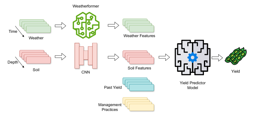
Figure 4: Soybean yield predictor architectures utilizing WeatherFormer. The weather measurements for the current year and the last few years are processed with WeatherFormer and the soil measurements are processed with a CNN reported in Khaki et al. (2020). Then the yield is predicted with either a linear layer or a transformer. The entire model is trained at once. Since yield for the current year is the target variable, it is replaced in the input with last year’s yield.

WeatherFormer+Linear Model: Weekly weather features for the current year and the past two years are processed with WeatherFormer separately and the dimension is reduced to 120 for each year. Next, the soil properties are processed with the CNN used in Khaki et al. (2020). These features are concatenated with management practices and past yields for each year. Since the current year’s yield is unknown, it is replaced by the last year’s yield. A single linear layer predicts yield from this input. This model highlights WeatherFormer’s direct impact but is suboptimal for yield prediction since the autoregressive pattern of soybean yield as shown in 2(a) is not taken into account.

WeatherFormer + Transformer: We replaced the last linear layer of the previous model with a transformer to capture the autoregressive trend of the data and then predicted the yield. We observed that 7 years of data gives the optimal performance on the validation set as opposed to 3 in the previous model.

Baseline Models: We tested three baseline models: a least squares linear regression model, the CNN-RNN model as proposed by Khaki et al. (2020), and a novel CNN-Transformer model.

The CNN-RNN model uses two separate CNNs to extract features from soil data across the depth dimension and weather data across the time dimension for the last three years. These features are then concatenated with the remaining data and passed through an LSTM to capture autoregressive patterns and then yield is predicted.

Next, we replaced the LSTM of the CNN-RNN model with a transformer encoder, since it has the self-attention mechanism and our novel spatiotemporal encoding can encode coordinates. This results in further improvement over the CNN-RNN model. We call this model CNN-Transformer in Table 1.

Optimization: All experiments used Adam optimizer, batch size 64, initial learning rate of 0.0005, 10-epoch warm-up, followed by exponential decay (factor 0.95). Models were trained for 40 epochs and evaluated on the validation set with the root mean square error (RMSE). The optimum number for past years’ data is different for each model and was optimized from 1 to 7 years. Each model took between 1 to 3 hours to train and evaluate on one NVIDIA V100 GPU.

6.2 Influenza Forecasting

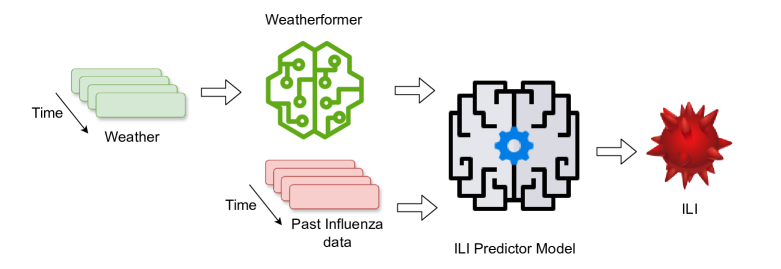
Figure 5: Influenza Like Illness (ILI) percent predictor architecture utilizing WeatherFormer. The weather measurements are first processed with WeatherFormer to extract useful features. These weather features and the past influenza data are processed by either a transformer to predict ILI percent for the next 10 weeks.

WeatherFormer+Transformer: Like the yield prediction problem, we process the weekly weather data with the WeatherFormer and concatenate with the historical influenza data (influenza like illness and number of total patients). This is then passed through a second transformer as shown in Figure 5 to predict the future influenza like illness (%) for the next 10 weeks. The second transformer has three layers and a hidden dimension of 64. The model parameters were chosen after testing with hidden dimension sizes of 8, 16, 32, and 64, and 1-4 layers. We also observed that adding the last known ILI value to the first predicted value of the model improved its performance.

Baseline Models:: For our baselines, we trained a least square linear regression model, an Autoregressive Integrated Moving Average (ARIMA) (Harvey, 1990) model, and two transformer encoder models: one was trained only with the past ILI percentage and the total number of patients for timeseries analysis of the data. The other transformer model utilized both the past influenza data and the weather data. Training two transformer models allows us to quantify the effects of weather on ILI percentage forecasting.

Optimization: Each model predicted the ILI percentage for a future period of 10 weeks. We used Mean Square Error (MSE) as the loss function for all the models, optimized using Adam optimizer with an initial learning rate of 0.0009 and for 30 epochs. We also employed an exponential learning rate scheduler that incorporated a 5-epoch warm-up phase followed by a decay factor of 0.95. All models took under 1 hour on one NVIDIA V100 GPU to train. Mean absolute error of 1, 5, and 10 weeks ahead predictions were reported in Table 2.

7 Results

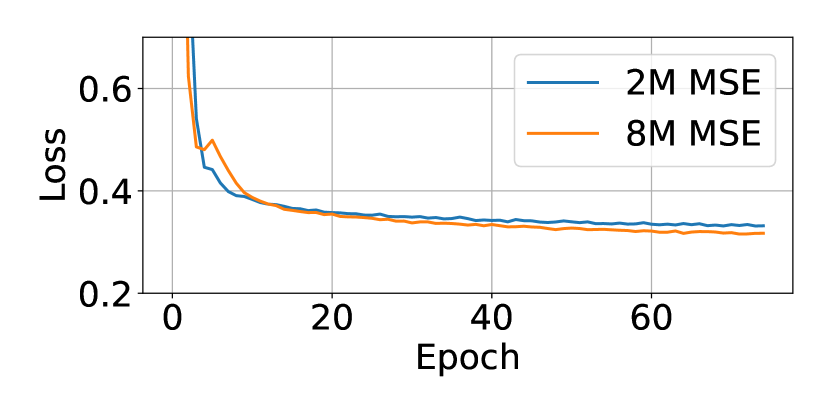
(a) Training.

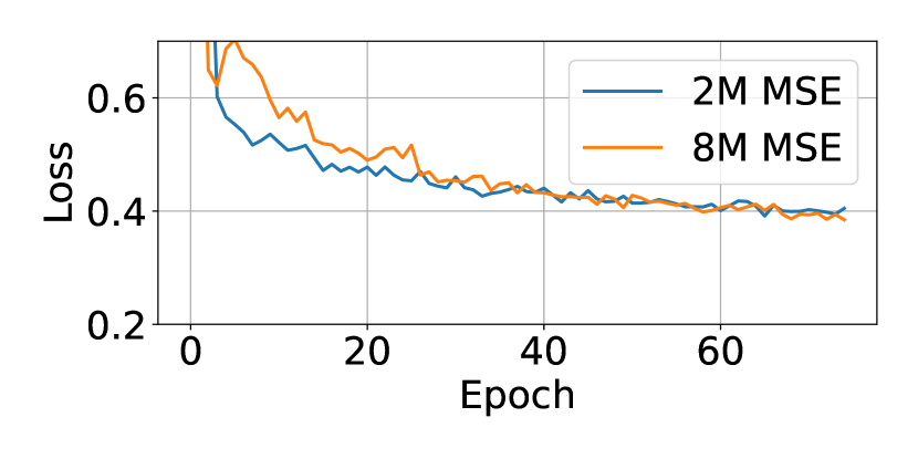
(b) Validation

Figure 6: Comparison between the 2M and 8M model losses during pretraining. Both models performed similarly in the validation dataset.

7.1 Pretraining

We did not observe performance improvement with larger sizes, which could be because larger models require more data to be effective. We also observed that the input scaler weights shifted away from 1 during training. For the 2M parameter model, the mean value for the input scalers was 0.346, and the mean value for the weekly input scalers was 0.682, suggesting that the model learned to differentiate between data from different temporal granularities.

7.2 Soybean Yield Prediction

In Table 1, we observe that the CNN-Transformer model performs better than the CNN-RNN model, suggesting the superiority of the transformer model to capture autoregressive patterns. On the other hand, WeatherFormer+Linear models show remarkable performance, due to superior weather feature extraction, but is still worse than the best model since autoregressive features were not captured well. Only when the WeatherFormer model and the transformer model are combined in WeatherFormer+Transformer models, the performance is optimum. Both the 8M and the 2M model performed similarly after finetuning.

Table 1: Comparison of Validation RMSE for county-level soybeans yield forecasting. The WeatherFormer models are pretrained and the mean and the standard deviation of the dataset are 38.5 Bu/Acre and 11.03 Bu/Acre, respectively.

Model	Validation RMSE
Linear Regression	6.90
CNN-RNN	5.50
CNN-Transformer	5.17
WF-2M + Linear	5.15
WF-8M + Linear	5.27
WF-2M + Transformer	4.83
WF-8M + Transformer	4.84

7.3 Influenza Forecasting

Table 2: Comparison of Validation MAE for ILI (%) forecasting. The target variable had a mean of 2.43% and a standard deviation of 1.73.

Model	+1 Week MAE	+5 Weeks MAE	+10 Weeks MAE
Linear Regression	0.392	0.437	0.456
ARIMA	0.219	0.409	0.427
Transformer (without weather)	0.193	0.328	0.371
Transformer	0.189	0.294	0.320
WF-2M + Transformer	0.186	0.277	0.297
WF-8M + Transformer	0.188	0.291	0.329

In Table 2, we observe that short-term influenza-like illness (ILI) behavior is predominantly influenced by recent influenza cases, as shown by the performance of the ARIMA models. However, a transformer encoder without weather can detect autoregressive features better, leading to better performance. Adding weather data improves the performance of the transformer for medium and long-term predictions. Additionally, WeatherFormer+Transformer-2M model shows considerable improvement over the base transformer model, further emphasizing the importance of good feature extraction. We also notice that the 8M pretrain model shows little to no improvement over the baseline transformer, suggesting that the model overfitted the small dataset.

8 Conclusion and Limitations

We pretrained two WeatherFormer models and showed that fine-tuning them improved performance in crop yield prediction and influenza forecasting. However, several limitations merit discussion. Firstly, the pretraining dataset could be expanded to include a larger area and ground-level measurements. The model hyperparameters can be tuned with an exhaustive grid search. And lastly, the model needs to be retrained every year on new weather data to stay relevant. We aim to address these limitations in future work.

Supplementary Material

9 Detailed Description of Datasets

9.1 Pretraining Dataset

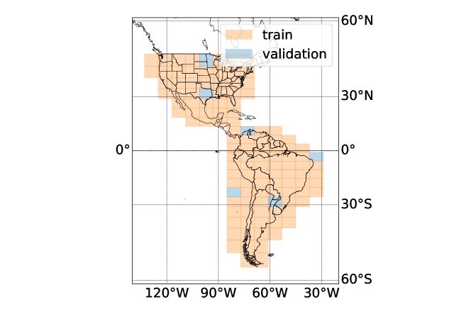
Figure 7: Map of the pretraining data. 5% of the grid rectangles were selected at random for validation and the rest were used for pretraining the model.

The dataset contained a small percentage of missing values, which were subsequently imputed using data from preceding years. After data collection, we applied the Tetens equation [Tetens, 1930] and the FAO Penman-Monteith formula [Ndulue and Ranjan, 2021], to calculate additional variables of interest such as saturation vapor pressure, vapor pressure deficit, and reference evapotranspiration. A complete list of all the weather measurements is given in LABEL:tab:weather_variables.

Additionally, we also computed weekly and monthly averages of the weather variables and added them to the datasets. Consequently, the WeatherFormer is trained on daily, weekly, and monthly granularities. The pretraining dataset in total had approximately $9.1$ billion floating point numbers. We used $95\%$ of the data for pretraining and $5\%$ data for validation as shown in Figure 7.

9.2 Soybean Yield Dataset

Data Collection

For the crop yield prediction problem, we used a soybean yield dataset introduced by Khaki et al. [2020]. This dataset contains county-level soybean yield for the nine states in the corn belt region of the United States from 1980 to 2018. Alongside soybean yield data, it also contains six weather variables (precipitation, solar radiation, snow water equivalent, maximum and minimum temperatures, and vapor pressure), soil profile across six depths for 10 characteristics (composition, bulk density, and organic matter content, etc) and management practices. Notably, the original paper reported results for 13 states and for corn and soybeans, but the publicly available dataset comprises data for only 9 states and only soybeans. Weather and practice data are provided weekly, whereas soil data lack a temporal component.

Train-Validation Split

The experiment was run five times and during each run, the data from randomly chosen seven states were used for training and the remaining two states were used for validation. The best Root Mean Square Error (RMSE) for the validation dataset from each of the five runs is averaged and reported.

It is important to note that the weather measurement source and granularity in this dataset are different from the pretraining data for WeatherFormer, and despite that the model showed considerable improvement over the baseline, suggesting a good understanding of the weather from pretraining.

9.3 Influenza Dataset

Another downstream predictive task we chose for the WeatherFormer was Influenza forecasting. The spread and severity of the influenza epidemic are strongly influenced by the mean temperature. Other weather variables such as humidity, precipitation, and wind speed also affect the process to varying degrees. Previously, several researchers, such as Amendolara et al. [2023] and Yang et al. [2023] have used weather as a data source for prediction. We decided to use only the mean temperature from NASA [2024] since our preliminary investigations on small models suggested that additional weather measurements introduce noise in the dataset.

Data Collection

We obtained our influenza dataset from Farrow et al. [2015], which includes weekly totals of Influenza-like Illness (ILI) cases and the percentage of ILI cases for New York City. The dataset spans 11 influenza seasons, from 2010-2011 to 2021-2022, and comprises weekly counts of patients, influenza cases, and the percentage of patients with ILI. We focused on predicting the percentage of ILIs among all patients. The dataset started on the week 40 of 2010. Due to a distribution shift attributed to COVID-19, data post-2020 were excluded.

For weather, we used our satellite-based weather data averaged over New York City. Amendolara et al. [2023] reported that temperature is a strong predictor of influenza cases followed by precipitation and wind speed. Average cooling and heating days are also important as these metrics relate to the time people spend indoors, a factor influencing transmission. We, however, discovered that only average temperature was sufficient for good prediction. Adding more measurements did not seem to improve the performance. This could be because our data source was from the satellite, which might be too imprecise for the task.

Train-Validation Split

We divided the remaining data into training and validation sets in four sequential phases: data from 2010 to 2015 was used for training and data from 2016 was used for validation. This pattern was repeated with training extended by one year each time, and validation occurring in the subsequent year. This resulted in four training and validation datasets. The best model’s performance on the validation sets was averaged. Following the methodology of Amendolara et al. [2023] and others in the field, we reported Mean Absolute Error (MAE) as our evaluation metric.

We evaluated each model using a rolling forecasting approach. Models received weather data and historical ILI cases for a fixed number of past weeks and were then tasked with predicting ILI cases for the subsequent 10 weeks without access to future weather information. Following each prediction cycle, the input window was shifted forward by one week, generating a new 10-week forecast that extended the previous one. This process was repeated which yielded 52 prediction tasks per year, each spanning 10 weeks.

We standardized all input data before training. We found that the historical window of input data critically influenced model performance. Consequently, we optimized this hyperparameter by exploring values within the range of ${105,110,115,\ldots,135}$ weeks. We also found that for the ARIMA model, the performance is given by $p=54$, $d=1$ and $q=1$.

10 Detailed Results for Finetuning Tasks

Table 3: Details of soybean yield prediction across across five validation sets. The dataset mean and standard deviation were 38.5 Bu/Acre and 11.03 Bu/Acre, respectively. The best performance in each dataset is highlighted.

	Validation RMSE
Model	Dataset 1	Dataset 2	Dataset 3	Dataset 4	Dataset 5
Linear Regression	5.52	7.28	8.44	7.05	6.21
CNN-RNN	4.74	5.14	6.94	5.37	5.31
CNN-Transformer	4.58	5.38	6.12	5.08	4.68
WF-2M + Linear	4.46	5.45	6.58	4.76	4.50
WF-8M + Linear	4.49	5.38	6.91	4.85	4.72
WF-2M + Transformer	4.13	5.16	5.88	4.79	4.17
WF-8M + Transformer	4.17	5.01	5.89	4.75	4.37

We present the detailed results for the soybean yield prediction task in Table 3. Every time 7 states were chosen at random for training and the remaining two were chosen for validation. The validation state pairs were (South Dakota, Iowa), (Nebraska, Minnesota), (North Dakota, Kansas), (North Dakota, Minnesota), and (North Dakota, Missouri).

Next, we present the detailed results for the influenza prediction in LABEL:tab:pretrained-flu-details. We observe that ILI in 2018 had a sharp peak (2(b)), which made the performance of all the models worse but in the other years, the model performances were more consistent.

Table 4: Details of influenza forecasting evaluation across four validation sets. The dataset mean and standard deviation were 2.43% and 1.73, respectively.

Model	+1 Week MAE	+5 Weeks MAE	+10 Weeks MAE
2016
Linear Regression	0.318	0.290	0.350
ARIMA	0.175	0.302	0.328
Transformer (without weather)	0.133	0.246	0.291
Transformer	0.124	0.243	0.245
WF-2M + Transformer	0.127	0.224	0.233
WF-8M + Transformer	0.130	0.231	0.275
2017
Linear Regression	0.341	0.356	0.350
ARIMA	0.179	0.297	0.298
Transformer (without weather)	0.172	0.272	0.301
Transformer	0.181	0.213	0.222
WF-2M + Transformer	0.178	0.209	0.195
WF-8M + Transformer	0.181	0.224	0.234
2018
Linear Regression	0.655	0.705	0.770
ARIMA	0.333	0.717	0.683
Transformer (without weather)	0.266	0.573	0.643
Transformer	0.273	0.530	0.558
WF-2M + Transformer	0.267	0.481	0.502
WF-8M + Transformer	0.273	0.502	0.527
2019
Linear Regression	0.256	0.398	0.354
ARIMA	0.188	0.321	0.398
Transformer (without weather)	0.199	0.223	0.249
Transformer	0.180	0.188	0.255
WF-2M + Transformer	0.173	0.192	0.256
WF-8M + Transformer	0.166	0.208	0.282

11 Ablation Studies

11.1 Pretraining

We believe it is important to test whether the performance improvement in Table 1 and Table 2 are due to the utilization of transformer architecture in weather feature extraction or due to pertaining. We hypothesize that the latter is true. To verify this hypothesis, we trained the same models from scratch, without loading the pretraining weights. Table 5 and Table 6 show that all models perform worse without pretraining.

Table 5: Comparison of Validation RMSE for county-level soybeans yield forecasting without pertaining. The large models overfit the training data and perform terribly on the validation dataset.

Model	Validation RMSE
Linear Regression	6.90
WeatherFormer-2M + Transformer	6.56
WeatherFormer-8M + Transformer	6.61

Table 6: Comparison of Validation MAE for ILI (%) forecasting. The larger models show worse performance due to overfitting.

Model	+1 Week MAE	+5 Weeks MAE	+10 Weeks MAE
Linear Regression	0.392	0.437	0.456
WF-2M + Transformer	0.188	0.295	0.318
WF-8M + Transformer	0.197	0.375	0.436

11.2 Training with Masked Language Modeling

We trained two additional WeatherFormer models of size 2M and 8M respectively with Masked Language Modeling. Following BERT, 15% of the tokens were masked with zero. We observe that the 8M parameter model struggles to fit the pretraining data with MLM. Previously, it was able to fit the data with Masked Feature Prediction and feature swapping, which resulted in the pretrained WeatherFormer-8M model used in previous experiements.

We tested different learning rates between 0.0005 and 0.001 and warmup periods but did not show improvement, suggesting a limitation of the MLM approach for pretraining on weather data.

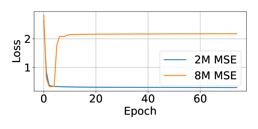
(a) Training.

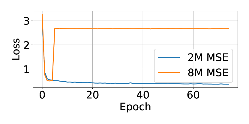
(b) Validation

Figure 8: Comparison between the 2M and 8M model losses during pretraining with MLM. The 8M model failed to converge.

12 Meteorological Equations

Weather measurements adhere to the principles of physics. When certain weather measurements are unavailable, they can be estimated using established meteorological equations. By leveraging these equations, we estimated additional atmospheric properties using collected data.

12.1 Tetens Equation

The Tetens equation, as described by Tetens [1930], offers a straightforward method to estimate the saturation vapor pressure ($e_{a}$) over liquid water or ice, contingent on the ambient temperature. For temperatures above freezing ($x>0^{\circ}C$, representing liquid water), the equation is:

$$e_{a}=0.6108\cdot\exp\left(\frac{17.27\cdot x}{x+237.3}\right)$$

Conversely, for temperatures at or below freezing ($x\leq 0^{\circ}C$, representing ice), the equation modifies to:

$$e_{a}=0.6108\cdot\exp\left(\frac{21.87\cdot x}{x+265.5}\right)$$

In these equations, $e_{a}$ represents the saturation vapor pressure in kPa, and $x$ denotes the temperature in degrees Celsius (${}^{\circ}C$).

12.2 FAO Penman-Monteith Equation

Accurate estimation of evapotranspiration (ET) is crucial for water resource management, agricultural planning, and understanding the hydrological cycle. The FAO Penman-Monteith equation [Ndulue and Ranjan, 2021] is widely accepted as the standard method for calculating reference evapotranspiration ($ET0$) from climatic data. The equation is expressed as:

$$ET0=\frac{0.408\Delta(R_{n}-G)+\gamma\frac{900}{T+273}u_{2}(e_{s}-e_{a})}{\Delta+\gamma(1+0.34u_{2})}$$

where:

• $ET0$ is the reference evapotranspiration (mm day^-1),

• $\Delta$ is the slope of vapor pressure curve (kPa ^∘C^-1),

• $R_{n}$ is the net radiation at the crop surface (MJ m^-2 day^-1),

• $G$ is the soil heat flux density (MJ m^-2 day^-1),

• $T$ is the mean daily air temperature at 2 m height (^∘C),

• $u_{2}$ is the wind speed at 2 m height (m s^-1),

• $e_{s}$ is the saturation vapor pressure (kPa),

• $e_{a}$ is the actual vapor pressure (kPa),

• $\gamma$ is the psychrometric constant (kPa ^∘C^-1).

This equation assumes a standard grass reference crop with an assumed height of 0.12 m, a fixed surface resistance of 70 sm^-1, and an albedo of 0.23.

13 List of Weather Measurements in the Pretraining Data

Here is a list of 31 daily weather measurements in the pretraining data. The first 28 measurements were downloaded from the NASA Power Project [NASA, 2024] from 1984 to 2022. The last three were predicted using the above equations.

Table 7: Descriptions of the 31 weather measurements and their units.

Measurement Name	Symbol	Unit
Temperature at 2 Meters	T2M	∘C
Temperature at 2 Meters Maximum	T2M_MAX	∘C
Temperature at 2 Meters Minimum	T2M_MIN	∘C
Wind Direction at 2 Meters	WD2M	Degrees
Wind Speed at 2 Meters	WS2M	m/s
Surface Pressure	PS	kPa
Specific Humidity at 2 Meters	QV2M	g/Kg
Precipitation Corrected	PRECTOTCORR	mm/day
All Sky Surface Shortwave Downward Irradiance	ALLSKY_SFC_SW_DWN	MJ/m2/day
Evapotranspiration Energy Flux	EVPTRNS	MJ/m2/day
Profile Soil Moisture (0 to 1)	GWETPROF	0 to 1
Snow Depth	SNODP	cm
Dew/Frost Point at 2 Meters	T2MDEW	∘C
Cloud Amount	CLOUD_AMT	0 to 1
Evaporation Land	EVLAND	kg/m2/s $\times 10^{6}$
Wet Bulb Temperature at 2 Meters	T2MWET	∘C
Land Snowcover Fraction	FRSNO	0 to 1
All Sky Surface Longwave Downward Irradiance	ALLSKY_SFC_LW_DWN	MJ/m2/day
All Sky Surface PAR Total	ALLSKY_SFC_PAR_TOT	MJ/m2/day
All Sky Surface Albedo	ALLSKY_SRF_ALB	0 to 1
Precipitable Water	PW	cm
Surface Roughness	Z0M	m
Surface Air Density	RHOA	kg/m3
Relative Humidity at 2 Meters	RH2M	0 to 1
Cooling Degree Days Above 18.3 C	CDD18_3	days
Heating Degree Days Below 18.3 C	HDD18_3	days
Total Column Ozone	TO3	Dobson units
Aerosol Optical Depth 55	AOD_55	0 to 1
Reference Evapotranspiration	ET0	mm/day
Vapor Pressure	VAP	kPa
Vapor Pressure Deficit	VAD	kPa

References

- Abdullah et al. (2022) NAMH Abdullah, NC Dom, SA Salleh, H Salim, and N Precha. The association between dengue case and climate: A systematic review and meta-analysis. One Health, 15:100452, Oct 2022. doi: 10.1016/j.onehlt.2022.100452.
- Ahamed et al. (2015) A.T.M.S. Ahamed, N.T. Mahmood, N. Hossain, M.T. Kabir, K. Das, F. Rahman, and R.M. Rahman. Applying data mining techniques to predict annual yield of major crops and recommend planting different crops in different districts in bangladesh. In Proceedings of the 2015 IEEE/ACIS 16th International Conference on Software Engineering, Artificial Intelligence, Networking and Parallel/Distributed Computing, SNPD 2015. IEEE, 2015. doi: 10.1109/SNPD.2015.7176185. URL https://doi.org/10.1109/SNPD.2015.7176185.
- Amendolara et al. (2023) A. B. Amendolara, D. Sant, H. G. Rotstein, et al. Lstm-based recurrent neural network provides effective short term flu forecasting. BMC Public Health, 23:1788, 2023. doi: 10.1186/s12889-023-16720-6. URL https://doi.org/10.1186/s12889-023-16720-6.
- Balting et al. (2021) D.F. Balting, A. AghaKouchak, G. Lohmann, et al. Northern hemisphere drought risk in a warming climate. npj Climate and Atmospheric Science, 4:61, 2021. doi: 10.1038/s41612-021-00218-2.
- Batra et al. (2021) Himanshu Batra, Narinder Singh Punn, Sanjay Kumar Sonbhadra, and Sonali Agarwal. BERT-Based Sentiment Analysis: A Software Engineering Perspective, page 138–148. Springer International Publishing, 2021. ISBN 9783030864729. doi: 10.1007/978-3-030-86472-9_13. URL http://dx.doi.org/10.1007/978-3-030-86472-9_13.
- Bi et al. (2024) Zhen Bi, Ningyu Zhang, Yida Xue, Yixin Ou, Daxiong Ji, Guozhou Zheng, and Huajun Chen. Oceangpt: A large language model for ocean science tasks, 2024.
- Brown et al. (2020) Tom B. Brown, Benjamin Mann, Nick Ryder, Melanie Subbiah, Jared Kaplan, Prafulla Dhariwal, Arvind Neelakantan, Pranav Shyam, Girish Sastry, Amanda Askell, Sandhini Agarwal, Ariel Herbert-Voss, Gretchen Krueger, Tom Henighan, Rewon Child, Aditya Ramesh, Daniel M. Ziegler, Jeffrey Wu, Clemens Winter, Christopher Hesse, Mark Chen, Eric Sigler, Mateusz Litwin, Scott Gray, Benjamin Chess, Jack Clark, Christopher Berner, Sam McCandlish, Alec Radford, Ilya Sutskever, and Dario Amodei. Language models are few-shot learners, 2020.
- CDC (2024) CDC. Weekly U.S. Influenza Surveillance Report. https://www.cdc.gov/flu/weekly/index.htm, 2024. [Accessed 08-05-2024].
- Christaki et al. (2020) Eirini Christaki, Panagiotis Dimitriou, Katerina Pantavou, and Georgios K. Nikolopoulos. The impact of climate change on cholera: A review on the global status and future challenges. Atmosphere, 11(5), 2020. ISSN 2073-4433. doi: 10.3390/atmos11050449. URL https://www.mdpi.com/2073-4433/11/5/449.
- Clark et al. (2020) Kevin Clark, Minh-Thang Luong, Quoc V. Le, and Christopher D. Manning. Electra: Pre-training text encoders as discriminators rather than generators, 2020.
- Devlin et al. (2019) Jacob Devlin, Ming-Wei Chang, Kenton Lee, and Kristina Toutanova. Bert: Pre-training of deep bidirectional transformers for language understanding, 2019.
- Eekhout and de Vente (2022) Joris P.C. Eekhout and Joris de Vente. Global impact of climate change on soil erosion and potential for adaptation through soil conservation. Earth-Science Reviews, 226:103921, 2022. ISSN 0012-8252. doi: https://doi.org/10.1016/j.earscirev.2022.103921. URL https://www.sciencedirect.com/science/article/pii/S0012825222000058.
- Fard et al. (2022) B. Jalalzadeh Fard, S. A. Hasan, and J. E. Bell. Climedbert: A pre-trained language model for climate and health-related text, 2022.
- Farrow et al. (2015) David C. Farrow, Logan C. Brooks, Ryan J. Tibshirani, and Roni Rosenfeld. Delphi epidata api. GitHub repository, 2015. URL https://github.com/cmu-delphi/delphi-epidata.
- Fernandez et al. (2023) Nigel Fernandez, Aritra Ghosh, Naiming Liu, Zichao Wang, Benoît Choffin, Richard Baraniuk, and Andrew Lan. Automated scoring for reading comprehension via in-context bert tuning, 2023.
- Harvey (1990) A.C. Harvey. Arima models. In John Eatwell, Murray Milgate, and Peter Newman, editors, Time Series and Statistics, The New Palgrave. Palgrave Macmillan, London, 1990. doi: 10.1007/978-1-349-20865-4_2. URL https://doi.org/10.1007/978-1-349-20865-4_2.
- Hochreiter and Schmidhuber (1997) Sepp Hochreiter and Jürgen Schmidhuber. Long short-term memory. Neural Computation, 9(8):1735–1780, 1997.
- Hoshen and Morse (2004) Moshe B Hoshen and Andrew P Morse. A weather-driven model of malaria transmission. Malaria Journal, 3:32, Sep 2004. doi: 10.1186/1475-2875-3-32.
- Jeong et al. (2016) J.H. Jeong, J.P. Resop, N.D. Mueller, D.H. Fleisher, K. Yun, E.E. Butler, and S.H. Kim. Random forests for global and regional crop yield predictions. PLoS ONE, 11(6), 2016. doi: 10.1371/journal.pone.0156571. URL https://doi.org/10.1371/journal.pone.0156571.
- Jia et al. (2024) C. Jia, Q. Cao, Z. Wang, A. van den Dool, and M. Yue. Climate change affects the spread of typhoid pathogens. Microbial Biotechnology, 17(2):e14417, 2024. doi: 10.1111/1751-7915.14417.
- Khaki et al. (2020) Saeed Khaki, Lizhi Wang, and Sotirios V. Archontoulis. A cnn-rnn framework for crop yield prediction. Frontiers in Plant Science, 10, 2020. ISSN 1664-462X. doi: 10.3389/fpls.2019.01750. URL https://www.frontiersin.org/journals/plant-science/articles/10.3389/fpls.2019.01750.
- Kingma and Ba (2017) Diederik P. Kingma and Jimmy Ba. Adam: A method for stochastic optimization, 2017.
- Kirezci et al. (2020) E. Kirezci, I.R. Young, R. Ranasinghe, et al. Projections of global-scale extreme sea levels and resulting episodic coastal flooding over the 21st century. Scientific Reports, 10:11629, 2020. doi: 10.1038/s41598-020-67736-6.
- Lam et al. (2023) Remi Lam, Alvaro Sanchez-Gonzalez, Matthew Willson, Peter Wirnsberger, Meire Fortunato, Ferran Alet, Suman Ravuri, Timo Ewalds, Zach Eaton-Rosen, Weihua Hu, Alexander Merose, Stephan Hoyer, George Holland, Oriol Vinyals, Jacklynn Stott, Alexander Pritzel, Shakir Mohamed, and Peter Battaglia. Graphcast: Learning skillful medium-range global weather forecasting, 2023.
- Lan et al. (2020) Zhenzhong Lan, Mingda Chen, Sebastian Goodman, Kevin Gimpel, Piyush Sharma, and Radu Soricut. Albert: A lite bert for self-supervised learning of language representations, 2020.
- Liu et al. (2019a) W. Liu, Q. Dai, J. Bao, W. Shen, Y. Wu, Y. Shi, K. Xu, J. Hu, C. Bao, and X. Huo. Influenza activity prediction using meteorological factors in a warm temperate to subtropical transitional zone, eastern china. Epidemiology and Infection, 147:e325, 2019a. doi: 10.1017/S0950268819002140. URL https://doi.org/10.1017/S0950268819002140. PMID: 31858924; PMCID: PMC7006024.
- Liu et al. (2019b) Yinhan Liu, Myle Ott, Naman Goyal, Jingfei Du, Mandar Joshi, Danqi Chen, Omer Levy, Mike Lewis, Luke Zettlemoyer, and Veselin Stoyanov. Roberta: A robustly optimized bert pretraining approach, 2019b.
- Man et al. (2023) Xin Man, Chenghong Zhang, Jin Feng, Changyu Li, and Jie Shao. W-mae: Pre-trained weather model with masked autoencoder for multi-variable weather forecasting, 2023.
- McFarland et al. (2020) B A McFarland, N AlKhalifah, M Bohn, J Bubert, E S Buckler, I Ciampitti, J Edwards, D Ertl, J L Gage, C M Falcon, S Flint-Garcia, M A Gore, C Graham, C N Hirsch, J B Holland, E Hood, D Hooker, D Jarquin, S M Kaeppler, J Knoll, G Kruger, N Lauter, E C Lee, D C Lima, A Lorenz, J P Lynch, J McKay, N D Miller, S P Moose, S C Murray, R Nelson, C Poudyal, T Rocheford, O Rodriguez, M C Romay, J C Schnable, P S Schnable, B Scully, R Sekhon, K Silverstein, M Singh, M Smith, E P Spalding, N Springer, K Thelen, P Thomison, M Tuinstra, J Wallace, R Walls, D Wills, R J Wisser, W Xu, C T Yeh, and N de Leon. Maize genomes to fields (g2f): 2014-2017 field seasons: genotype, phenotype, climatic, soil, and inbred ear image datasets. BMC Research Notes, 13(1):71, 2020. doi: 10.1186/s13104-020-4922-8.
- NASA (2024) NASA. NASA Power API, 2024. URL https://power.larc.nasa.gov/docs/referencing/.
- Ndulue and Ranjan (2021) Emeka Ndulue and Ramanathan Sri Ranjan. Performance of the fao penman-monteith equation under limiting conditions and fourteen reference evapotranspiration models in southern manitoba. Theoretical and Applied Climatology, 143(3):1285–1298, Feb 2021. ISSN 1434-4483. doi: 10.1007/s00704-020-03505-9. URL https://doi.org/10.1007/s00704-020-03505-9.
- Nguyen et al. (2023) Tung Nguyen, Johannes Brandstetter, Ashish Kapoor, Jayesh K. Gupta, and Aditya Grover. Climax: A foundation model for weather and climate, 2023.
- Osthus and Moran (2021) D. Osthus and K.R. Moran. Multiscale influenza forecasting. Nature Communications, 12:2991, 2021. doi: 10.1038/s41467-021-23234-5. URL https://doi.org/10.1038/s41467-021-23234-5.
- Osthus et al. (2019) D. Osthus, J. Gattiker, R. Priedhorsky, and S. Y. Del Valle. Dynamic bayesian influenza forecasting in the united states with hierarchical discrepancy (with discussion). Bayesian Analysis, 14:261–312, 2019.
- Pathak et al. (2022) Jaideep Pathak, Shashank Subramanian, Peter Harrington, Sanjeev Raja, Ashesh Chattopadhyay, Morteza Mardani, Thorsten Kurth, David Hall, Zongyi Li, Kamyar Azizzadenesheli, Pedram Hassanzadeh, Karthik Kashinath, and Animashree Anandkumar. Fourcastnet: A global data-driven high-resolution weather model using adaptive fourier neural operators. arXiv preprint arXiv:2202.11214, 2022.
- Radford et al. (2018) Alec Radford, Karthik Narasimhan, Tim Salimans, and Ilya Sutskever. Improving language understanding by generative pre-training, 2018.
- Ruß and Kruse (2010) G. Ruß and R. Kruse. Regression models for spatial data: An example from precision agriculture. In Proceedings of the Advances in Data Mining Applications and Theoretical Aspects, pages 450–463, 2010. doi: 10.1007/978-3-642-14400-4_35. URL https://doi.org/10.1007/978-3-642-14400-4_35.
- Ruß et al. (2008) G. Ruß, R. Kruse, M. Schneider, and P. Wagner. Data mining with neural networks for wheat yield prediction. In Lecture Notes in Computer Science (including subseries Lecture Notes in Artificial Intelligence and Lecture Notes in Bioinformatics), volume 5077 LNAI, pages 47–56, Berlin, Heidelberg, 2008. Springer Berlin Heidelberg. doi: 10.1007/978-3-540-70720-2_4. URL https://doi.org/10.1007/978-3-540-70720-2_4.
- Scarselli et al. (2009) Franco Scarselli, Marco Gori, Ah Chung Tsoi, Markus Hagenbuchner, and Gabriele Monfardini. The graph neural network model. IEEE Transactions on Neural Networks, 20(1):61–80, 2009. doi: 10.1109/TNN.2008.2005605.
- Tetens (1930) O. Tetens. Über einige meteorologische begriffe (on some meteorological terms). Z. Geophys., 6:297–309, 1930.
- Vaswani et al. (2017) Ashish Vaswani, Noam Shazeer, Niki Parmar, Jakob Uszkoreit, Llion Jones, Aidan N. Gomez, Lukasz Kaiser, and Illia Polosukhin. Attention is all you need, 2017.
- Webersinke et al. (2022) Nicolas Webersinke, Mathias Kraus, Julia Anna Bingler, and Markus Leippold. Climatebert: A pretrained language model for climate-related text, 2022.
- Wu et al. (2021) Dongxia Wu, Liyao Gao, Xinyue Xiong, Matteo Chinazzi, Alessandro Vespignani, Yi-An Ma, and Rose Yu. Deepgleam: A hybrid mechanistic and deep learning model for covid-19 forecasting, 2021.
- Yang et al. (2023) L. Yang, G. Li, J. Yang, T. Zhang, J. Du, T. Liu, X. Zhang, X. Han, W. Li, L. Ma, L. Feng, and W. Yang. Deep-learning model for influenza prediction from multisource heterogeneous data in a megacity: Model development and evaluation. Journal of Medical Internet Research, 25:e44238, Feb 2023. doi: 10.2196/44238. URL https://doi.org/10.2196/44238. PMID: 36780207; PMCID: PMC9972203.
- Zhu et al. (2020) Jinhua Zhu, Yingce Xia, Lijun Wu, Di He, Tao Qin, Wengang Zhou, Houqiang Li, and Tie-Yan Liu. Incorporating bert into neural machine translation, 2020.
- Zimmer and Yaesoubi (2020) Christoph Zimmer and Reza Yaesoubi. Influenza forecasting framework based on Gaussian processes. In Hal Daumé III and Aarti Singh, editors, Proceedings of the 37th International Conference on Machine Learning, volume 119 of Proceedings of Machine Learning Research, pages 11671–11679. PMLR, 13–18 Jul 2020. URL https://proceedings.mlr.press/v119/zimmer20a.html.