Modelling between- and within-season trajectories in elite athletic performance data
Running title: Seasonal effects in athletic performance data
Abstract
Athletic performance follows a typical pattern of improvement and decline during a career. This pattern is also often observed within-seasons as athlete aims for their performance to peak at key events such as the Olympic Games or World Championships. A Bayesian hierarchical model is developed to analyse the evolution of athletic sporting performance throughout an athlete’s career and separate these effects whilst allowing for confounding factors such as environmental conditions. Our model works in continuous time and estimates both the average performance level of the population, , at age and how each -th athlete differs from the average . We further decompose into changes from season-to-season, termed the between-season performance trajectory, and within-season performance trajectories which are modelled by
a constrained Bernstein polynomial. Hence, the specific focus of this project is to identify the differences in performance that exist both between and within-seasons for each athlete. For the implementation of the model an adaptive Metropolis-within-Gibbs algorithm is used. An illustration of algorithm’s performance on 100 metres and 200 metres freestyle swimming in both female and male athletes is presented.
Keywords: Longitudinal modelling; Bernstein polynomial; global-local prior; Bayesian inference; Splines.
1 Introduction
The availability of large databases of elite athlete performance allows the modelling of performance levels over an athlete’s career, which we will call an athlete’s career performance trajectory. Results from these models can be used for short-term predictions (such as the results of future events), long-term predictions (such as talent spotting through prediction of career trajectories at the start of an athlete’s career), or retrospective analysis (understanding how an athlete’s performance level evolved over their career). Understanding the variation across athletes and time is critical to effectively answer these questions. For example, research has suggested that race-to-race variation in an athlete’s performance is an important determinant for success (Hopkins and Hewson, 2001) since it provides an estimate for the smallest important change in performance and is therefore crucial for sport scientists when prescribing training or monitoring individual athletes career trajectories. Indeed, the modelling of career progression has been used to establish likely age of peak performance (Allen et al., 2014) and chances of medal success at the Olympic Games (Pyne et al., 2004). Being able to estimate within athlete variability between seasons is important for assessing long-term performance changes. When modelling within-season performance trajectories of centimeter, gram, second sports, they often follow a cyclical pattern, dictated by events of high importance (e.g. Olympics or World Championships) within the competitive calendar. However, this pattern may differ between years since events such as the Olympic games or World Championships do not occur every year. We will refer to these as within-season performance trajectories and consider the variation in these between seasons within athletes as well as between athletes.
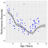
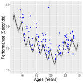
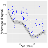
The modelling of elite athlete performance data is challenging since it is measured irregularly with potential confounders, a trend over time, possible cyclical components, non-Gaussian errors and sparsity of observations for some athletes. The graphs in Figure 2 show the observed performance and fitted career performance trajectory with 95% credible interval for 100 metre freestyle swimmers (bottom row for each swimmer). There is clear evidence of a trend in performance (termed the between-season performance trajectory within this paper) and a cyclical component which corresponds to variations over a season (termed within-season performance trajectory within this paper). This is particularly clear for Swimmer 1 whose performance level improves from an average of 57 seconds at 15 to 53 seconds at 25 but who also improves within seasons by about 2 seconds due to habitual training and peaking for defined events within the year. The graphs also illustrate the non-Gaussian errors which are positively skewed with a possibly heavy right-hand tail.
The irregular observations leads us to build a continuous-time longitudinal model. Longitudinal models were originally proposed for sporting performance data by Berry et al. (1999), who build a linear mixed model with a common effect of age (usually called the ageing function), an individual effect and a season effect. We build on Griffin et al. (2022) who include a fourth-order polynomial ageing function, an athlete-specific effect over time and allows for confounders such as meteorological factors (e.g. wind speed or temperature) or geographical factors (e.g. altitude). Athletic performance as a function of age typically follows a “u” shape (Stival et al., 2023) with athlete’s improving to a mid-career peak (Griffin et al., 2022) followed by deterioration. The age of peak performance often occurs between the ages 23 to 28 but can differ between sports, gender and individuals (Griffin et al., 2022). The departure of an individual athlete’s career performance trajectory from the population ageing function leads to a trend component within the model. Some athletes are better able to maintain their performance levels in late career whereas others will develop more quickly at the start of their career. The observational variation is often also skewed and, potentially, heavy tailed due athletes having a higher chance of underperforming rather than overperforming to the same degree. The model of Griffin et al. (2022) was adequate for the disciplines considered in their paper (weightlifting and 100 metres sprint), but ignore the effects of annual performance cycles.
There has been some previous research using a simpler mixed-modelling approach with scalar individual and season effects in an attempt to capture both within and between season variability in athlete performance (Paton and Hopkins, 2005; Trewin et al., 2004; Bullock et al., 2009; Pyne et al., 2004). However, this often leads to an overestimation of variability between consecutive performances because variability is calculated for all competition within a season regardless of how the competitions were distributed within a given season (Malcata and Hopkins, 2014). To best of our knowledge, there has been little attempt to model changes in performance levels over a season.
In this study, we develop a method for modelling the changes in performance over a season using a constrained Bernstein polynomial (Wang and Ghosh, 2012) and extend the model of Griffin et al. (2022). We also increase the flexibility of the model in three additional directions. Firstly, we investigate the use of a distribution which allows for different tail heaviness in each tail. Secondly, we use a B-spline to have a fully flexible population ageing function. Thirdly, we address the sparsity of observations for some athletes a global-local shrinkage priors in a normal hierarchical model. This encourages parts of the hierarchy to be strongly shrunk towards the mean unless the data supports differences.
The paper is organized as follows: Section 2 explains how the model is formed. In Section 3 inference is presented. Section 4 includes application to 100 metres freestyle for female and male swimmers. Lastly, in Section 5, a discussion is provided. Appendices present the full Markov chain Monte Carlo (MCMC) for Bayesian inference, as well as an application to 200m freestyle for female and male swimmers.
2 Model
We assume that each season is one year long (although the approach could be easily adapted to other season lengths). Suppose that the -th athlete has observations for seasons, we define to be a vector of performances observed at times with confounders in the -th season. Suppose that the -th athlete is aged at the start of their first season. Griffin et al. (2022) decompose the observed performance as a function of age into a population component, individual component, effects of confounders and an observational error. We change their notation to allow for a cyclical within-season component by indexing the individual component by season as well as the individual. This leads to the model
| (1) |
where models the average population performance trajectory and (for ) is an individual performance trajectory (i.e. the difference between the -th athlete’s performance level and the average population performance trajectory) in the -th season, is a vector of effects of the confounders, and are i.i.d. observation errors.
We depart from Griffin et al. (2022) in the modelling of , and the distribution of . Firstly, we model using a cubic B-splines (De Boor, 1972). Let be a cubic B-spline with knots are knot positions (which we position equally spaced between the minimum and maximum ages in the database), then we use
| (2) |
where are spline coefficients and is a length scale (which controls the shape of the fitted function ). This is a more flexible form than the polynomial regression considered in Griffin et al. (2022).
It is convenient to define an athlete’s career-wide individual performance trajectory, by joining the individual performance trajectories in each season, as
This is modelled as a sum of a between-season performance trajectory which allows for season-to-season variation and within-season performance trajectories which allow for the variation within a season. We write to be the between-season performance trajectory in season . For identifiability, we assume that so that and . Wang and Ghosh (2012) show how a restricted Bernstein polynomial (RBP) basis of order can meet this condition and provide a flexible form. We use the sum of RBP bases of degree 2 to (we use ) to model the within-season performance trajectory
| (3) |
where
The individual performance trajectory at the start of each season is modelled using a random walk with increments for . We model the initial value by and the increments by . This allows for heavy tails in the distribution of initial individual performance level and for abrupt changes in the underlying individual performance level . The between-season performance trajectory is an interpolation of the individual performance at the start of each season
It is useful to also define athlete-specific trajectories which include the average population performance level . We refer to
as the -th athlete’s combined performance trajectory, and
as the -th athlete’s combined between-season performance trajectory since it adjusts the combined performance trajectory for the within-season effects.
Griffin et al. (2022) assume that the regression error follows a skew- distribution. This allows for both skewness and heavy tails which are observed in elite athlete performance data due to larger probabilities of extreme underperformance compared to overperformance. However, it assumes that the heaviness of tails is the same in both negative and positive directions. We consider a model which allows differences in the heaviness of the two tails and find clear evidence of a difference in our empirical data study. We assume the generalisation of the skew- distribution to . For events where better performance leads to a smaller observed performances (such as timed events), we assume that , , , and all elements are independent. This reverts to a skew- distribution if (and so ). In events where better performance leads to a larger observed performances (for example, weight lifted or distance jumped), we assume that . The heaviness of the left-hand tail is controlled by the minimum of and and the heaviness of the right-hand tail by .
3 Inference
We make Bayesian inference using a hierarchical model with MCMC. The use of a hierarchical model allows us to make inference about an athlete’s within-season performance trajectory with a small number of observations (or, indeed, none) in a season using a global-local shrinkage prior (Bhadra et al., 2019).
The prior for the coefficients of the RBP basis, are given a hierarchical prior. We define ,
where the length of , and is defined to be . The hierarchical structure introduces and which can be interpreted as average coefficients over all seasons for the -th athlete and average coefficients over all seasons and all athletes respectively. This allows us to also estimate the average within-season performance trajectory at the population level by
and for the -th athlete by
The global-local shrinkage prior on the variances of each level of the hierarchy allow the effects to be shrunk towards the corresponding mean. Small values of imply that the within-season coefficients are similar across all seasons and a small value of imply that the -th athlete’s average coefficients are close to the corresponding population average.
The Bayesian model is completed by specifying priors for all other parameters. We use global-local shrinkage priors for and to avoid overfitting. We use a standardized Lomax prior for the precision with shape parameter which we write and which has the density
The parameter controls the tails and the distribution does not have a mean if . We use which is closely related to the objective Lomax prior for scale parameters of Walker and Villa (2021) and the normal-exponential-gamma (Griffin and Brown, 2011). It has a heavy tail and finite mass at zero (unlike the half-Cauchy prior on the variance which underlies the horseshoe prior (Carvalho et al., 2010) which has infinite density at zero). We find that the horseshoe can lead to instability in the MCMC algorithm. Our priors are
We use a hierarchical model for the scale of the observation error for each athlete
The athlete ages usually cover a span of about 25 years and so we use knots in the B-spline and . We give an informative prior to the skewness parameter , . All other parameters are given vague priors:
The model in (1) with the choice of basis function model for and and distribution for can be written in the following form
| (4) |
where is a -dimensional column vector of all performances in the -th season of the -th athlete, is -dimensional matrix whose -th entry is value of -th performance and -th B-spline evaluated at the age, within the season with vector of length . of the observed confounders is a -dimensional matrix whose -th row is the value of all confounders for the -th performance with the associated vector of length , is a -dimensional matrix whose only non-zero entries in the -th row are in the -th position and in the -th position and , is -dimensional matrix whose -th entry is the -th performance of the -th value of the Bernstein polynomial associated with and evaluated at the time, within the season. This is a linear model which has a simple structure, where and are time-invariant, are conditionally independent given and has a random walk prior. We use blocking and interweaving in the Gibbs sampler to derive an algorithm which gives reasonable performance. The full MCMC algorithm is described in Appendix B.
The hierarchical model for the within-season performance trajectory allows us to estimate functional effects at the season, athlete and population level. It is useful to also have univariate measures of the sizes of these effects. To establish these measures, it’s useful to note the following results for the RBP in (3) (a proof is given in the appendix A). Suppose that then
-
(a)
,
-
(b)
where
The variability over different seasons for the -th athlete can be measured by considering the differences between the within-season performance trajectory for the -th season and the average within-season performance trajectory for the -th athlete which is
Taking the expectation of with respect to the prior distribution of leads to the expression
which we call the within-season variability for the -th athlete. In a similar way, we can summarise the size of the difference in effect between an athlete’s average within-season performance trajectory and the average within-season performance trajectory across all athletes using the measure
Taking the expectation of with respect to the prior distribution of leads to the expression
which we call the average effect size for the -th athlete.
4 Results
We applied our model to data from 100 metre and 200 metre freestyle swimming for both females and males. We selected the 500 swimmers for each combination of distance and gender with the fastest personal bests from 2008 to 2023 and with a minimum of five performances.
| Event | Number of | Number of | Number of Performances | ||
|---|---|---|---|---|---|
| Performances | Athletes | per Athlete | |||
| Median | Minimum | Maximum | |||
| 100 metres, female | 23669 | 500 | 37.5 | 5 | 267 |
| 100 metres, male | 23440 | 500 | 38 | 5 | 191 |
| 200 metres, female | 21112 | 500 | 33 | 5 | 274 |
| 200 metres, male | 19696 | 500 | 32 | 5 | 162 |
Summaries of the number of performances and athletes are provided in Table 1. The data includes performances in both 25 and 50 metre long pools, and so we include a dummy variable for 25 metre pool performances as a confounder. To make performances comparable when presenting data in the paper figures, we plot performances in 25 metres pools adjusted by the posterior mean of this pool effect. In this section, we will concentrate on results for both female and male 100 metre freestyle swimming. The results for female and male 200 metre freestyle are provided in Appendix C.
| Females | Males | |
|---|---|---|
| 100 metres |  |
 |
| 200 metres |  |
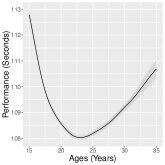 |
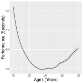
Figure 1 shows the estimated average population performance trajectory as a function of age. For all ages, the trajectory follows a reverse J shape as in Griffin et al. (2022) with performance rapidly improving between 15 and 20, peaking around 24 (in both men and women), and subsequently slowly decreasing. The improvement in performance between 15 and 20 is noticeably smaller for women ( seconds) than men ( seconds).
| Female | ||
|---|---|---|
| Swimmer 1 | Swimmer 2 | Swimmer 3 |
 |
 |
 |
 |
 |
 |
| Male | ||
| Swimmer 4 | Swimmer 5 | Swimmer 6 |
 |
 |
 |
 |
 |
 |
We find that there is a strong within-season effect in these data sets. Indeed, Figure 2 shows combined performance trajectories and combined between-season performance trajectories for three female and three male swimmers. The figure demonstrates a clear effect of seasonality, with a pattern of performance improvement and deterioration over each season in all swimmers. For example, Swimmer 1 improves by about 2 seconds over the course of a season and Swimmer 4 improves by about 3 seconds over the course of a season. This magnitude of improvement is reasonably consistent season on season, but there are clearly seasons where performance changes are greater than others. Plots of the combined performance trajectory (Figure 2 top row) demonstrates the trend in each swimmer’s performance level over the course of their career. For example, it can be seen that Swimmer 3’s performance level improves by about 3.5 seconds between 15 and 21 years of age.
| Female | ||
|---|---|---|
| Swimmer 1 | Swimmer 2 | Swimmer 3 |
 |
 |
 |
 |
 |
 |
| Male | ||
| Swimmer 4 | Swimmer 5 | Swimmer 6 |
 |
 |
 |
 |
 |
 |
To better understand the within-season effect, we plot the average within-season performance trajectory at the population level, the individual athlete level and the season level for each athlete for the six swimmers in figure 3. These are plotted in terms of performance improvement. In swimming improved performance corresponds to faster times and so the plots show , and . The population trajectory is fairly flat across the season with performance improving by about 0.3 seconds between January and April and staying relatively constant from April to September. The results show variability in the estimated athlete-level within-season performance trajectory. Some swimmers, such as 2 and 6, have estimates which closely follow those from the population-level. Other swimmers, however, show much greater changes in performance over a season. Swimmers 1, 3, and 4 show improvements of 2, 1 and 2.5 seconds respectively with the peak performance occurring in September. The estimated within-season performance trajectories are fairly close to the athlete-level estimates (particularly, for swimmers 2, 3, and 5) showing little variability from season to season in their within-season performance trajectories. The athletes with larger changes in their performance over the season also show more variability between seasons (e.g. swimmers 1 and 4) and so the level of variability appears to be driven by the size of the within-season improvement.
| Females | Males |
|---|---|
 |
 |
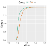
Figure 4 shows the empirical distribution function of the posterior median values of the within-season variability () and the average effect size () for females and males. The distribution is similar for both females and males and so we concentrate on the results for female. Both distributions have a very heavy right-tail so that a few effects have much larger values of and than others. The distribution of is shifted to the left of the distribution of indicating that the within-season variability tends to be smaller than the average effect size. In other words, the season-on-season variability within a swimmer tends to be smaller than the variability between swimmers. This indicates that swimmers have some ability to control how their performance levels evolve over a season through the training process, and are able to replicate that improvement in different seasons.
| Females | Males |
|---|---|
 |
 |
 |
 |
Figure 5 shows the posterior mean estimated error densities for female and male 100 metre freestyle swimmers. The distribution is clearly positively skewed and there is also evidence of a difference in the heaviness of the left-hand and right-hand tails. The logarithm of the posterior mean more clearly shows the differences in the weight of the two tails. The right-hand tail is clearly much heavier than the left-hand tail which is close to normal.
5 Discussion
In this work we have developed a Bayesian longitudinal model which can account for the variation in performance change within a season across population-level, athlete-level and within-season (i.e. within athlete). An application to freestyle swimming data shows that there is substantial variation between swimmers and between seasons with some having a clear pattern of peaking for major events (e.g. Olympics Games and World Championships) which usually occur during the summer months (July - August). We use a B-spline to model the population-level effect of age and an error distribution which allows for skewness and different heaviness of the left and right tail. We find that the population-level effect of age follows the expected reverse J shape in freestyle swimming with a difference between the improvement in performance of females and males in years 15 to 23. We find that the error distribution has a much lighter left tail than right tail. The left tail represents better than expected performance whereas the right tail represents worse than expected performance. The result suggests that swimmers are much less likely to have a performance that is substantially worse than expected, rather than one that is substantially better than expected. One explanation is that elite athletes generally perform close to their optimal level and so improvements are much harder to achieve than poor performances (which can be due to many factors including things such as poor race execution, illness and injury). Although we have implemented techniques to enhance the speed of our calculations, we fit our model using MCMC which is computationally expensive. Our future work will be focused on techniques, such as variational Bayes, to greatly reduce the time needed to fit the model.
Acknowledgements
This research was supported by Partnership for Clean Competition grant 514.
References
- Allen et al. (2014) Allen, S. V., T. J. Vandenbogaerde, and W. G. Hopkins (2014). Career performance trajectories of Olympic swimmers: benchmarks for talent development. European Journal of Sports Science 14, 643–651.
- Atchadé and Rosenthal (2005) Atchadé, Y. F. and J. S. Rosenthal (2005). On adaptive Markov chain Monte Carlo algorithms. Bernoulli 11, 815–828.
- Atchadé and Fort (2010) Atchadé, Y. and G. Fort (2010). Limit theorems for some adaptive MCMC algorithms with subgeometric kernels. Bernoulli 16, 116–154.
- Berry et al. (1999) Berry, S. M., C. S. Reese, and P. D. Larkey (1999). Bridging Different Eras in Sports. Journal of the American Statistical Association 94, 661–676.
- Bhadra et al. (2019) Bhadra, A., J. Datta, N. G. Polson, and B. Willard (2019). Lasso meets horseshoe: A survey. Statistical Science 34, 405–427.
- Bullock et al. (2009) Bullock, N., J. Gulbin, D. T. Martin, and A. Ross (2009). Talent indentification and deliberate programming in skeleton: Ice novice to Winter Olympian in 14 months. Journal of Sports Science 27, 397–404.
- Carvalho et al. (2010) Carvalho, C. M., N. G. Polson, and J. G. Scott (2010). The horseshoe estimator for sparse signals. Biometrika 97, 465–480.
- De Boor (1972) De Boor, C. (1972). On calculating with B-splines. Journal of Approximation Theory 6, 50–62.
- Griffin and Brown (2011) Griffin, J. E. and P. J. Brown (2011). Bayesian adaptive lassos with non-convex penalization. Australian and New Zealand Journal of Statistics 53, 423–442.
- Griffin et al. (2022) Griffin, J. E., L. C. Hinoveanu, and J. G. Hopker (2022). Bayesian modelling of elite sporting performance with large databases. Journal of Quantitative Analysis in Sports 18, 253–267.
- Griffin and Stephens (2013) Griffin, J. E. and D. A. Stephens (2013). Advances in Markov chain Monte Carlo. In P. Damien, P. Dellaportas, N. G. Polson, and D. A. Stephens (Eds.), Bayesian Theory and Applications. Oxford: Oxford University Press.
- Hopkins and Hewson (2001) Hopkins, W. G. and D. J. Hewson (2001). Variability of competitive performeance of distance runners. Medicine & Science in Sports & Exercise 33, 1588–1592.
- Makalic and Schmidt (2016) Makalic, E. and D. F. Schmidt (2016). A simple sampler for the horseshoe estimator. IEEE Signal Processing Letters 23, 179–182.
- Malcata and Hopkins (2014) Malcata, R. M. and W. G. Hopkins (2014). Variability of competitive performance of elite athletes: a systematic review. Sports Medicine 44, 1763–74.
- Paton and Hopkins (2005) Paton, C. D. and W. G. Hopkins (2005). Combining explosive and high-resistance training improves performance in competitive cyclists. Journal of Strength & Conditioning Research 19, 826–830.
- Pyne et al. (2004) Pyne, D., C. Trewin, and W. Hopkins (2004). Progression and variability of competitve performance of Olympic swimmers. Journal of Sports Science 22, 613–620.
- Stival et al. (2023) Stival, M., M. Bernardi, M. Cattelan, and P. Dellaportas (2023). Missing data patterns in runners’ careers: do they matter? Journal of the Royal Statistical Society Series C: Applied Statistics 72(1), 213–230.
- Trewin et al. (2004) Trewin, C. B., W. G. Hopkins, and D. B. Pyne (2004). Relationship between world-ranking and Olympic performance of swimmers. Journal of Sports Science 22, 339–345.
- Walker and Villa (2021) Walker, S. G. and C. Villa (2021). An Objective Prior from a Scoring Rule. Entropy 23(7), 18.
- Wang and Ghosh (2012) Wang, J. and S. K. Ghosh (2012). Shape restricted nonparametric regression with Bernstein polynomials. Computational Statistics and Data Analysis 56, 2729–2741.
- Yu and Meng (2011) Yu, Y. and X.-L. Meng (2011). To center or not to center: That is not the question — An ancillarity–sufficiency interweaving strategy (ASIS) for boosting MCMC efficiency. Journal of Computational and Graphical Statistics 20, 531–570.
Appendix A Proof of results for RBP
We can show that
-
•
-
•
Appendix B MCMC sampler
Suppose that there are athletes. We use the linear model representation in (4) to derive the Gibbs sampler:
In a similar way to Makalic and Schmidt (2016) for horseshoe priors, we can write the Lomax prior for , , and as
We use the notation , and to be represent the -th row of , and respectively.
The sampler uses a combination of joint updates and interweaving (Yu and Meng, 2011) to achieve good performance. We provide the full conditional distribution if it has a known form, otherwise, we provide the density of the full conditional. For these parameters, we use adaptive Metropolis-Hastings random walk updates (see Griffin and Stephens, 2013, for a review). For univariate parameters, we use an adaptive random walk tuned to an acceptance rate of 0.3 (Atchadé and Rosenthal, 2005). For multivariate parameters, we initially use an adaptive random walk on each component of the parameter then we switch to the ASWAM algorithm (Atchadé and Fort, 2010) which proposes from a random walk on whole parameter vector whose covariance matrix is a tuning parameter multiplied by the covariance matrix of the parameters estimated using the previous MCMC samples. The steps of the Gibbs sampler are given below.
Jointly update , , , , and
We update the parameters , , and in blocks before sampling , and . For , , and , we use a Metropolis-Hastings random walk and update in the blocks , and for (which involves updates). The likelihood for these parameters is evaluated integrating over , and and is proportional to
where
-
1.
Sample :
where
-
2.
Sample :
where
Update
Jointly update , and
We jointly update these parameters by first updating using a Metropolis-Hastings random walk marginalizing over and and then sampling and . The likelihood depends on through the matrices . The full conditional density is proportional to:
where
We sample and conditional on from the full conditional
Update
where
Update
where
Jointly update , and using an interweaving step
Let . Interweaving introduces an extra step in the Gibbs sampler where we update the parameter using the model re-parameterised from to . The full conditional distribution is
where
The use of the re-parameterisation in this interweaving step leads to deterministic updates where is the previous value of
where represents the value of before updating in this step.
Update
where
Update
The full conditional density is proportional to
Update
Update
The full conditional density is proportional to
Update
where
Update
Update
Update
Update
Update
Update
Update
Update
Jointly update and
We first update using an adaptive Metropolis-Hastings random walk and then update for all possible values of , and . The full conditional density of is proportional to
For all possible values of , , and , sample
Update and
We first update using an adaptive Metropolis-Hastings random walk and then update for all possible values of , and . The full conditional density of is proportional to
For all possible value of , and , sample
Update and
We first update using an adaptive Metropolis-Hastings random walk and then update for . The full conditional density of is proportional to
For , sample
Update and
We first update using an adaptive Metropolis-Hastings random walk and then update for all possible values of and . The full conditional density of is proportional to
For all possible value of and , sample
Appendix C Additional results for 200m Freestyle
| Female | ||
|---|---|---|
| Swimmer 1 | Swimmer 2 | Swimmer 3 |
 |
 |
 |
 |
 |
 |
| Male | ||
| Swimmer 4 | Swimmer 5 | Swimmer 6 |
 |
 |
 |
 |
 |
 |
| Female | ||
|---|---|---|
| Swimmer 1 | Swimmer 2 | Swimmer 3 |
 |
 |
 |
 |
 |
 |
| Male | ||
| Swimmer 4 | Swimmer 5 | Swimmer 6 |
 |
 |
 |
 |
 |
 |
| Females | Males |
|---|---|
 |
 |
| Females | Males |
|---|---|
 |
 |
 |
 |