Imaginary past of a quantum particle moving on imaginary time
Abstract
The analytical continuation of classical equations of motion to complex times suggests that a tunnelling particle spends in the barrier an imaginary duration . Does this mean that it takes a finite time to tunnel, or should tunnelling be seen as an instantaneous process? It is well known that examination of the adiabatic limit in a small additional AC field points towards being the time it takes to traverse the barrier. However, this is only half the story. We probe the transmitted particle’s history, and find that it remembers very little of the field’s past behaviour, as if the transit time were close to zero. The ensuing contradiction suggests that the question is ill-posed, and we explain why.
I Introduction
Recent advances in atto-second laser techniques AT have revived the interest in the nearly century-old question McColl . Is tunnelling infinitely fast as was suggested, for example, in references zero1 ,zero2 , or does a particle spend in the barrier a finite duration, as was argued, e.g., in nzero1 ,nzero2 ? The question itself is somewhat vague, since there is no consensus as to how this duration should be defined (for recent and not-so-recent reviews of the subject see Rev1 -Rev2 ).
In dealing with a conceptual difficulty it is often helpful to resort to a simple yet representative model. One such model is that of a semiclassical particle transmitted across a smooth potential barrier. It is well known that the particle’s motion can be described by the equations of classical mechanics analytically continued into the complex time plane Pop , McL . This provides a formal yet not a particularly useful answer: The particle spends in a classically forbidden region an imaginary duration . The result clearly needs an interpretation, and in Ref.BL the authors, who studied the adiabatic limit of tunnelling in the presence of a small AC field, concluded that must after all be the time the particle spends in the barrier region BL1 . In this paper we show that analysis of BL , BL1 (the model was recently revisited in Poll1 ) presents only one side of the story. Examining instead the part of the time dependent potential actually experienced by a tunnelling particle equally suggests that the duration spent inside the barrier must in fact be close to zero. We argue that the question is ill-posed, and explain why it should be so. Before addressing the case of tunnelling we briefly review the classically allowed case, where both approaches agree.
II The classically allowed case
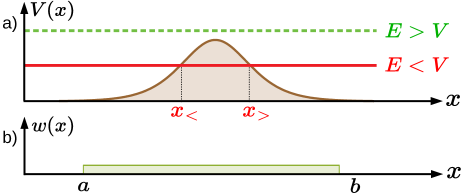
Consider a particle of energy and mass , incident from the left on a stationary potential barrier , assuming . A small time dependent perturbation [ for , and otherwise]
| (1) |
is added in a region (see Fig.1). The particle’s wave function satisfies a Schrödinger equation ()
| (2) |
which can be solved by expanding the wave function in powers of , , where
| (3) |
where is the Feynman propagator FeynH for the motion in a potential . Evidently, may depend on (i.e., “remember”) all the values of , , although its behaviour in the distant past is expected to be less important. Defining an effective region of integration for an oscillatory integral is notoriously difficult (for more details see, e.g., DSX1 ). However, a more precise estimate is available if varies slowly compared to the particle’s de-Broglie wavelength. Then the terms in the perturbation series can be obtained by invoking the semiclassical approximation for FeynH , and evaluating the -integrals by the stationary phase method. If, in addition, in Eq.(2) also varies slowly in (except maybe at the endpoints and ), the series can be summed (for details see Appendix A). Thus, for an , “downstream” from the region which contains , one finds
| (4a) | ||||
| (4b) | ||||
| (4c) | ||||
and
| (5) |
is the particle’s momentum. In Eq. (4c), is the classical trajectory of a particle with energy , which arrives in at a time , implicitly defined by
| (6) |
and , are the moments when the trajectory enters and leaves the region , respectively.
Equations (4)-(6), whose validity is discussed in Ref. DSac and in Appendix B, have a simple interpretation. We are interested in a particle of energy found (“post-selected”) in a given location at a time . In the (semi)classical limit, the particle’s past is well defined: it has been following a classical trajectory . Accordingly, the particle may probe the potential only at the moment passes through that location. Clearly it spends inside the region a duration
| (7) |
It is easy to devise simple tests which would convince one that this is, indeed, the case. Consider the case of a time dependent potential “step”
| (8) |
and ask how slowly must vary for the particle to “see” a static potential, fixed, say, at the moment it leaves the region . Choosing , helps discount the time of travel from to , and expanding in a Taylor series, , one finds
| (9) |
The first term is the desired adiabatic approximation. The second one can be neglected if it is small compared to unity. For a harmonic perturbation this means , where , [cf. Eq.(40)].
As expected, adiabaticity is achieved provided the particle crosses the region so quickly, the oscillating potential has no time to change.
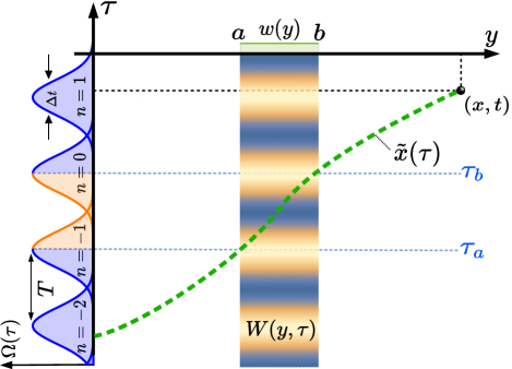
Our second test is even simpler. Suppose in Eq. (8) is a sequence of Gaussian pulses of various magnitudes ,
| (10) | |||
provided by the experimenter. How many of these pulses affect the phase of the wave function at some ? The answer is, of course, those which overlap with the interval , since
| (11) |
Figure 2 shows the case where the particle leaves the region at , is equal to the separation between the pulses, , and . Their relative contributions are given in Table 1 for future comparison with the classically forbidden case.
| Allowed | Forbidden | |
|---|---|---|
The same conclusion can also be drawn from inspecting directly observable quantities. The simplest choice would be the probability density , but it remains unchanged by the presence of . The probability current at , may, however, be affected since can alter the particle’s velocity. Thus, for the extra term added to we find
| (12) | |||
Since is the additional force acting on the particle, the last integral is the work done to change its kinetic energy. The first term in brackets accounts for the jolts experienced by the particle as it enters and leaves the region, and is the only remaining contribution in the case of a step-like potential (8). The current at depends on only for , which provides yet another proof of the particle’s presence between and during this interval. Note that there is no extra current in the adiabatic limit , since for a static potential the net work done by the extra force acting on the particle is null. However, for in Eq. (8), approaches its zero limit as , and the classical duration spent in is again the relevant time parameter.
In summary, both tests are consistent with a classical picture of a particle which enters the region at , leaves at , and spends there a duration . The tests can also be applied in the classically forbidden case, and we will do it next.
III The classically forbidden case (tunnelling)
The formal derivation in the case is remarkably similar, if one extends the definition of the particle’s momentum to the region where as ( for )
| (13) |
It is easy to check (see Appendices A and B), that the wave function of a particle transmitted across the barrier is still given by Eq.(4) where
| (14a) | ||||
| (14b) | ||||
and and are the turning points where vanishes (see Fig.1). The main difference with the classically allowed case is that now integration over is performed along a contour in the complex -plane, defined by,
| (15) |
The contour, shown in Fig.3, runs along the real -axis while , then parallel to the imaginary axis for between and , and finally parallel to the real axis for . It is readily seen that on Eq. (15) defines a real-valued trajectory (), shown in Fig. 3 for an Eckart potential Eck_P .
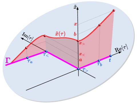
The trajectory satisfies the Newton’s equation along each segment of the contour, and was proven by McLaughlin McL to be the real-valued critical path of the Feynman path integral analytically continued to complex times. The time integrals in the power series for can now be evaluated by the saddle point method (see Appendix A), and the summed series bears similarity to that in Eq.(4).
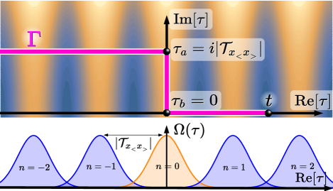
There is, however, an apparent difficulty in trying to establish when exactly the tunnelling particle was present in the classically forbidden region, since a perturbing potential (8), restricted to the sub-barrier region, , , is probed along the vertical part of the contour in Fig. 4. For a particle, just emerging from the barrier at , , , the integration is along the imaginary time axis, and one has
| (16) | |||
An experimenter, controlling the real-time behaviour of the perturbing potential given by (8), is unlikely to be satisfied with an explanation that “the particle is present inside the barrier between the times and ”, and would want to know what this could mean in practice. In case of tunnelling, he/she will need to look no further than the particle density at
| (17) |
now modified by the perturbation, since is complex valued.
As in our first adiabatic test, one can ask how slowly should vary on the real -axis, for to be given by its expression for a static step-like potential , in which constant is replaced by for each . Expanding, as before, in a Taylor series around yields
| (18) |
Now with the adiabatic limit is reached provided the first and the second terms on the right-hand side of Eq. (18) are of order of unity, and much less than unity, respectively. This leads to a condition
| (19) |
first obtained in Ref. BL , albeit in a slightly different form. Its similarity to the classically allowed case convinced the authors of Refs. BL , BL1 that must be “the time a tunnelling particle spends in the barrier region”. We will, however, reserve judgement until submitting the tunnelling particle to our second test.
Suppose again that the potential in the classically forbidden region is modified by a series of Gaussian pulses (10). If is indeed the duration spent in the barrier region, the particle exiting the barrier at and must be affected by what happened in the barrier between and . This, however, does not happen, as we will show next. Calculating at and with the help of Eqs.(16) and (17) yields
| (20) | |||
Unlike in the classical case, increasing (e.g., by making the barrier broader) does not let the particle experience more pulses, since remains of order of , small if . Moreover, the approximation used in deriving Eqs. (16) and (17) requires , so that, by necessity, , which leaves the only non-negligible contribution. The particle appears to have “no memory” of other narrow pulses, and the experimenter would measure practically the same density by applying only the pulse. The ratios for
| (21) |
are listed in Table 1 alongside the results obtained earlier for the classically allowed case. With our choice of parameters, in the classical regime the pulses with and contribute equally to in the exponent in Eq.(4a). With tunnelling, only the pulse affects the particle emerging from the barrier, which should not be the case for a particle spending in the sub-barrier region.
There is obviously a discrepancy with what was learnt in the adiabatic test, and it is easy to see why. In our first test, the rate of change of a slowly varying analytical function along any direction in the complex -plane is determined by the same , which accounts for the similarity between Eqs.(9) and (18). However, in the second test, analytic continuation of a Gaussian is such that making barrier broader does not let the particle explore its behaviour further into the past. (The reader may note a certain parallel with the Hartman effect Hart , whereby the arrival of a tunnelled particle is not delayed by increasing the barrier’s width.) The effect persists if the ratio is made smaller (see Appendix B), which suggests that the duration the particle spends in the barrier must be zero, or very close to zero. One can keep the ratio constant, and reduce so more pulses fit into the interval ( can be chosen to ensure .) Still, only the pulse will be taken into account, even though now the pulse belongs to a more recent past.
IV Conclusions and discussion
Our aim here is not to provide yet another “evidence” of tunnelling being “instantaneous”, but rather to gain a broader view of the problem itself.
Two equally feasible (at least in principle) experiments give the same answer in the classically allowed case.
Both suggest that the interaction of a classical particle with a small field is governed by the duration , spent by its trajectory region where the field is applied.
Alice and Bob, making different tests in their respective laboratories, can agree about this point.
This is not so in the case of tunnelling. An extension of the classical equations of motion to complex time still yields a
single “duration” , but now it is imaginary, . Is tunnelling instantaneous, since ,
or does it take seconds to cross the barrier region?
Both tests can be performed also in the tunnelling regime, but this time the results appear to contradict each other.
With the classical picture still in mind, Alice’s would find her adiabatic test pointing towards a finite tunnelling time, . This is the well-known
Büttiker-Landauer result, often interpreted as the true duration of a tunnelling process BL . On the other hand Bob, who studies the
“memory” of a tunnelled particle, must conclude that the duration spent in the barrier is much shorter than
, and is in fact close to zero.
If both Alice’s in Bob’s results are correct, the concept of a well-defined classical-like tunnelling time must be at fault.
The problem is well known in quantum measurement theory.
A quantity, uniquely defined on a single (classical) trajectory must become indeterminate if two or more paths leading to the
particle’s final condition interfere FeynL . An attempt to measure it without destroying the interference yields only a complex “weak value” (see, e.g., Ref. DSwv and references therein).
Such is the time measured by a weakly coupled Larmor clock Larm1 -Larm2 , .
The spin of the clock results rotated both in the plane perpendicular to the magnetic field by
an angle (as in the classical case), but also in the plane parallel to the field, by (a new non-classical feature).
Moreover, in the semiclassical limit one has , whereas (the reader may begin to see a connection).
Alice, who has measured , could argue that “tunnelling is instantaneous”, since the spin has not rotated in the way it does in the classical case. Bob, who has measured , could argue that tunnelling “takes a finite time” since, after all, the field caused the spin rotate, albeit in a different manner. So, which part of the complex represents the physical “duration spent in the barrier”?
In general, neither nor is a valid candidate since, for some initial and final particle’s states, both can turn out to be negative DSsw , DSel . The absolute value, (known as the “Büttiker time” BL2 ) is indeed real, but can exceed the time the particle was in motion DSsw , DSel . The reason for this strange behaviour is the Uncertainty Principle FeynL which, among other things, forbids knowing the time spent in the barrier in a situation where different durations interfere to produce the tunnelling amplitude DSel .
If the theory does not allow one to describe classically forbidden tunnelling in terms of a classical-like duration, it is rather pointless to ask whether or not this non-existent duration should be zero. One can try to approach the question from the operational side, by adopting to the tunnelling regime experiments, known to yield the classical duration in the classically allowed case. The problem is, one will obtain results which, if interpreted at face value, appear to support either of the conflicting viewpoints. In this paper we have shown that the same is also true for the Büttiker-Landauer model BL , which employs a time-modulated barrier, instead of an external clock. A reasonable way out of the contradiction is to accept that, in the absence of a classical-like tunnelling time, different experiments may yield different quantities with units of time Poll2 . The nature and properties of such quantities can then be analysed individually by the methods of elementary quantum mechanics.
One may be disappointed to learn that the object of a long standing search may not exist or, what is worse, exists in many conflicting shapes and forms. Perhaps a different approach would deliver a well defined tunnelling time? This seems unlikely. The “phase time” (see, e.g., Ref. Rev1 ), associated with the transmission of broad wave packets, can be analysed along the same lines as the Larmor time DSX1 , DSno , DSX2 . Moreover, the above analysis emphasises the importance of a conventional trajectory for the existence of a unique duration spent in a given region of space. Even when such a trajectory exists along a contour displaced into the complex time plane (cf. Fig. 3), the resulting complex duration looses the properties of a physical time interval.
Acknowledgements
D.S. acknowledges financial support by Grant No. PID2021-126273NB-I00 funded by MICINN/AEI/10.13039/501100011033 and by “ERDF A way of making Europe”, as well as by the Basque Government Grant No. IT1470-22.
A.U. and E.A. acknowledge the financial support by the Ministerio de Ciencia y Innovación (MICINN, AEI) of the Spanish Government through BCAM Severo Ochoa accreditation CEX2021-001142-S and PID2019-104927GB-C22, PID2022-136585NB-C22 grants funded by MICIU/AEI/10.13039/501100011033, as well as by the Basque Government through the BERC 2022-2025 Program, IKUR Program, ELKARTEK Programme (Grants No. KK-2022/00006 and No. KK-2023/00016).
Appendix A Quantum perturbation theory
We need to solve, in the semiclassical limit, a Schrödinger equation
| (22) |
where vanishes unless .
A.1 The classically allowed case
Expanding in a Born series, , one has
| (23) | |||
where
| (24) |
and . The Green’s function is simply related to the Feynman propagator FeynH as
| (25) |
where is for , and otherwise. The propagator has a well known classical limit FeynH , where
| (26) |
is the classical action evaluated along the trajectory connecting the points and .
As , the time integral for can be evaluated by the stationary phase method. The corresponding condition ensures that the main contribution to the integral comes from a time at which a particle with energy , destined to arrive at , passes through the point ,
| (27) |
With a pre-exponential factor evaluated at , the first term of the series [see Eq.(23)] takes the form
| (28) |
Repeating the calculation, using a relation
| (29) |
and summing the series for yields
| (30) |
where, explicitly,
| (31) |
Changing the variable yields the last of Eqs.(4). A classical particle “probes” a time dependent perturbation as it follows its trajectory.
A.2 The classically forbidden case
The case where a particle tunnels across a barrier can be treated in a similar manner (at least in one spatial dimension), as was shown by McLaughlin in Ref. McL . After applying the standard connection formulae and multiplying the result by the zero-order wave function can be written as
| (32) |
where between turning points and and otherwise. As was shown in Ref. McL , the semiclassical limit of analytically continued into the complex plane of still given by , with evaluated along the real valued path along a complex contour connecting complex with a real . The integrals (23) can now be evaluated by the saddle point method. For the complex saddle at [cf. Eq. (3.9) of Ref. McL ]
| (33) | |||
lies in the upper half of the complex -plane. For an lying between the turning points and (see Fig.1) one has
| (34) |
and for there is real stationary point
| (35) |
The only difference from McLaughlin’s derivation McL is the presence of in the integrand, which needs to be evaluated at the saddle. Acting as before, we obtain Eq.(30) with given by the last of Eqs.(32) and a complex valued
| (36) |
which after a change of variables becomes Eq.(5), where it is understood that the “time” varies along the complex contour , defined by Eq.(15). A tunnelling particle “moving on complex time along a real valued trajectory” McL “probes” a time dependent perturbation analytically continued away from the real time axis.
Appendix B Classical perturbation theory
The result (30) can be obtained in a different and, perhaps, a more illustrative manner.
B.1 The classically allowed case
Making the usual ansatz (and restoring ) , one finds that satisfies the Hamilton-Jacobi equation,
| (37) |
where for and otherwise. If is sufficiently small, it can be neglected in the pre-exponential factor , but not in the exponent, where one writes . Equation (37) can be solved iteratively. Setting yields a first order equation for ,
| (38) |
which has a particular solution
| (39) |
. The higher-order terms, with , can be neglected if they are small compared to unity. This requires
| (40) |
which, in turn, imposes restrictions on the magnitude and the rate of change of a perturbation .
Setting and applying (39) for yields
.
This agrees with the correct semiclassical form [],
provided
| (41) |
The limit on how fast can change with time for the approximation to remain valid is obtained by considering the first order term of the Born series. Writing one notes that after absorbing (emitting) quanta for should contain terms like . This agrees with
| (42) |
obtained from Eqs.(4) and (39) provided the absorbed energy is small compared to the particle’s kinetic energy, . If is the time scale upon which changes, the condition reads
| (43) |
B.2 The classically forbidden case
in Eq.(39) remains a continuous solution of Eq.(38) if is defined by Eq.(13). Thus, in Eq.(4) is valid, provided the presence of does not alter the matching rules near the turning points and , where conditions (41) and (43) are clearly violated. However, a more detailed analysis (see Ref. DSac and references therein) shows that the rules remain unchanged near a linear turning point, , .
The simplest illustration is given by the case of a broad rectangular barrier, , where the matching rules at depend on the particle’s energy (see Ref. DSac ). Condition (43), applied on both sides of the turning point, eliminates this dependence, leaving still given by Eq. (4), apart from an overall energy-dependent factor. Suppose, for simplicity, that , and . We are interested in the ratio between the pulse’s width and the modulus of the complex time, . A typical absorbed energy is obviously of order of , and from (43) we have
| (44) |
However, is the sub-barrier action, which is always large in the semiclassical limit considered here. This shows that the used approximation (4) is valid if the pulse is significantly shorter than the Büttiker-Landauer time BL .
References
- (1) M. Hentschel, R. Kienberger, Ch. Spielmann, G. A. Reider, N. Milosevic, T. Brabec, P. Corkum, U. Heinzmann, M. Drescher and F. Krausz, Attosecond metrology, Nature 414, 509 (2001).
- (2) L. A. MacColl, Note on the transmission and reflection of wave packets by potential barriers, Phys. Rev. 40, 621 (1932).
- (3) L. Torlina, F. Morales, J. Kaushal, I. Ivanov, A. Kheifets, A. Zielinski, A. Scrinzi, H. G. Muller, S. Sukiasyan, M. Ivanov, et al., Interpreting attoclock measurements of tunnelling times, Nature Physics, 11, 503 (2015).
- (4) U. S. Sainadh, H. Xu, X. Wang, A. Atia-Tul-Noor, W. C. Wallace, N. Douguet, A. Bray, I. Ivanov, K. Bartschat, A. Kheifets, et. al., Attosecond angular streaking and tunnelling time in atomic hydrogen, Nature, 568, 75 (2019).
- (5) N. Camus, E. Yakaboylu, L. Fechner, M. Klaiber, M. Laux, Y. Mi, K. Z. Hatsagortsyan, T. Pfeifer, C. H. Keitel, and R. Moshammer, Experimental evidence for quantum tunneling time, Phys. Rev. Lett. 119, 023201 (2017).
- (6) R. Ramos, D. Spierings, I. Racicot and A. M. Steinberg, Measurement of the time spent by a tunnelling atom within the barrier region, Nature 583, 529 (2020).
- (7) E. H. Hauge and J. A. Støevneng, Tunnelling times: a critical review, Rev. Mod. Phys. 61, 917 (1989).
- (8) R. Landauer and Th. Martin, Barrier interacting time in tunnelling, Rev. Mod. Phys. 66, 217 (1994).
- (9) C. A. A. de Carvalho, H. M. Nussenzweig, Time delay, Phys. Rep. 364, 83 (2002).
- (10) V. S. Olkhovsky, E. Recami and J. Jakiel, Unified time analysis of photon and particle tunnelling, Phys. Rep. 398, 133 (2004).
- (11) H. G. Winful, Tunneling time, the Hartman effect, and superluminality: A proposed resolution of an old paradox, Phys. Rep. 436, 1 (2006).
- (12) A. Landsman and U. Keller, Attosecond science and the tunnelling time problem, Phys. Rep. 60, 1 (2015).
- (13) G.E. Field, On the status of quantum tunnelling time, Eur. J. Phil. Sci. 12, 57 (2022).
- (14) V. S. Popov, V. P. Kuznetsov, and A.M. Perelomov, Quasiclassical approximation for nonstationary problems, Sov. Phys. JETP, 26, 222 (1968), [Zh. Eksp. Teor. Fiz. 53, 331 (1967)].
- (15) D. W. McLaughlin, Complex time, contour independent path integrals, and barrier penetration, J. Math. Phys. 13, 1099 (1972).
- (16) M. Büttiker and R. Landauer, Traversal Time for Tunneling, Phys. Rev. Lett. 49, 1739 (1982).
- (17) M. Büttiker and R. Landauer, Traversal time for tunneling, edited by P. Grosse (Springer, Berlin, Heidelberg, 1985), in Festkörperprobleme 25, Advances in Solid State Physics, Vol. 25, pp. 711-717.
- (18) R. Ianconescu, and E. Pollak, Determination of the mean tunneling flight time in the Büttiker-Landauer oscillating-barrier model as the reflected phase time, Phys. Rev. A 103, 042215 (2021).
- (19) R. P. Feynman, and A. R. Hibbs, Quantum Mechanics and Path Integrals (Dover, New York, 1965)
- (20) X. Gutiérrez de la Cal, M. Pons, and D Sokolovski, Speed-up and slow-down of a quantum particle, Sci. Rep. 12, 3842 (2022).
- (21) D. Sokolovski, Resonance tunneling in a periodic time-dependent external field, Phys. Rev. B 37, 4201 (1988).
- (22) The trajectory shown in Fig. 3 is calculated numerically for an Eckart potential at for . The imaginary time spent in the barrier can be analytically calculated to be given by the turning points .
- (23) T. E. Hartman, Tunneling of a Wave Packet, J. Appl. Phys. 33, 3427 (1962).
- (24) D. Sokolovski and E. Akhmatskaya, An even simpler understanding of quantum weak values, Ann. Phys. 388, 382 (2018).
- (25) A. I. Baz’, Ya. B. Zeldovich and A. M. Perelomov, Scattering, Reactions and Decay in Non-relativistic Quantum Mechanics, (Israel Program for Scientific Translations, Jerusalem, 1969).
- (26) M. Büttiker, Larmor precession and the traversal time for tunneling, Phys. Rev. B, 27, 6178 (1983).
- (27) D. Sokolovski and L.S. Baskin, Traversal time in quantum scattering, Phys. Rev. A, 36, 4604 (1987).
- (28) J.P. Falck and E.H. Hauge, Larmor clock reexamined, Phys. Rev. B, 38, 3287 (1988).
- (29) C. R. Leavens and G. C. Aers, Larmor-clock transmission times for resonant double barriers, Phys. Rev. B, 40, 5387 (1989).
- (30) C. S. Park, 3D Larmor clock and barrier interaction times for tunneling, Phys. Lett. A 377, 741 (2013).
- (31) D. Sokolovski, The Salecker-Wigner-Peres clock, Feynman paths, and one tunnelling time that should not exist, Phys. Rev. A 96, 022120 (2017).
- (32) D. Sokolovski and E. Akhmatskaya, Tunnelling times, Larmor clock, and the elephant in the room, Sci. Rep. 11, 10040 (2021).
- (33) Feynman, R. P., Leighton, R., Sands, M., The Feynman Lectures on Physics III (Dover Publications, Inc., New York, 1989), Chap.1: Quantum Behavior.
- (34) T. Rivlin , E. Pollak, and R. S. Dumont. Comparison of a direct measure of barrier crossing times with indirect measures such as the Larmor time, New J. Phys. 23, 063044 (2021).
- (35) D. Sokolovski and E. Akhmatskaya, No time at the end of the tunnel, Commun. Phys. 1, 47 (2018).
- (36) X. Gutiérrez de la Cal, M. Pons, and D Sokolovski, Quantum measurements and delays in scattering by zero-range potentials, Entropy. 26, 75 (2024).