Dual-Delayed Asynchronous SGD for Arbitrarily Heterogeneous Data

Abstract

We consider the distributed learning problem with data dispersed across multiple workers under the orchestration of a central server. Asynchronous Stochastic Gradient Descent (SGD) has been widely explored in such a setting to reduce the synchronization overhead associated with parallelization. However, the performance of asynchronous SGD algorithms often depends on a bounded dissimilarity condition among the workers’ local data, a condition that can drastically affect their efficiency when the workers’ data are highly heterogeneous. To overcome this limitation, we introduce the dual-delayed asynchronous SGD (DuDe-ASGD) algorithm designed to neutralize the adverse effects of data heterogeneity. DuDe-ASGD makes full use of stale stochastic gradients from all workers during asynchronous training, leading to two distinct time lags in the model parameters and data samples utilized in the server’s iterations. Furthermore, by adopting an incremental aggregation strategy, DuDe-ASGD maintains a per-iteration computational cost that is on par with traditional asynchronous SGD algorithms. Our analysis demonstrates that DuDe-ASGD achieves a near-minimax-optimal convergence rate for smooth nonconvex problems, even when the data across workers are extremely heterogeneous. Numerical experiments indicate that DuDe-ASGD compares favorably with existing asynchronous and synchronous SGD-based algorithms.

1 Introduction

In traditional machine learning, training often occurs on a single machine. This approach can be restrictive when handling large datasets or complex models that demand substantial computational resources. Distributed machine learning overcomes this constraint by utilizing multiple machines working in parallel. This method distributes the computational workload and data across several nodes or workers, enabling faster and more scalable training.

We focus on the most common distributed machine learning paradigm, known as the data parallelism approach. In this setup, the training data are distributed among multiple workers, with each worker independently conducting computations on its local data. As an extension of stochastic gradient descent (SGD) used on a single machine, synchronous SGD (Cotter et al., 2011; Dekel et al., 2012; Chen et al., 2016; Goyal et al., 2017) stands as a prominent example of data-parallel training algorithms. In synchronous SGD, the server broadcasts the latest model to all workers, who then simultaneously compute stochastic gradients using their respective datasets. After local computation, these workers send their stochastic gradients back to the central server. The server then aggregates these stochastic gradients and updates the global model accordingly.

However, variations in computation speeds and communication bandwidths across workers, typically due to differences in hardware, are common. In synchronous SGD, this disparity forces all workers to wait for the slowest one to complete its computations before proceeding to the next iteration. This issue, often referred to as the straggler effect, leads to significant idle times, severely limiting the efficiency and scalability of the approach. To address this problem, asynchronous SGD (ASGD) algorithms have been extensively studied to mitigate the synchronization overhead among workers. Since nodes operate independently, each can proceed at its own pace without waiting for others. This attribute is especially beneficial in ad-hoc clusters or cloud environments where hardware heterogeneity is prevalent (Assran et al., 2020).

The primary challenge faced by asynchronous training is that its efficiency can be compromised by data heterogeneity. This issue arises because fast workers are able to send more frequent updates to the server, while slower workers contribute less frequently. Consequently, the training process may become biased, as the data from fast and slow workers are not equally represented in the server’s model updates. Recent research efforts have addressed the problem of data heterogeneity in ASGD (Gao et al., 2021; Mishchenko et al., 2022; Koloskova et al., 2022; Islamov et al., 2024). These studies focus on the convergence properties of ASGD under conditions where the dissimilarity of local objective functions is bounded. However, if the local datasets are highly heterogeneous, leading to significant differences in local objective functions, then the convergence performance of these algorithms can be substantially reduced.

1.1 Our Contributions

In this paper, we tackle the above limitations in existing ASGD algorithms. Our main contributions are summarized as follows:

1. We propose the dual-delayed ASGD (DuDe-ASGD) algorithm for distributed training, with the following key features:

   1. DuDe-ASGD aggregates the stochastic gradients from all workers, which are computed based on both stale models and stale data samples. This leads to a dual-delayed aggregated gradient at the server, contrasting sharply with traditional ASGD algorithms that use stale models but fresh data samples for each iteration.

   2. DuDe-ASGD operates in a fully asynchronous manner, meaning that the server updates the global model as soon as it receives a stochastic gradient from any worker, without the need to wait for others. Additionally, DuDe-ASGD can be readily adapted to semi-asynchronous implementations, which allows it to balance the advantages of both synchronous and asynchronous training methods, demonstrating its high flexibility.

   3. Although DuDe-ASGD requires aggregation of stochastic gradients from all workers in every iteration, it can be implemented incrementally by storing each worker’s latest stochastic gradient, maintaining a per-iteration computational cost comparable to traditional ASGD algorithms.

2. Through a careful analysis accounting for the time lags inherent in the dual-delayed system, we demonstrate that DuDe-ASGD achieves a near-minimax-optimal convergence rate for solving general nonconvex problems under mild assumptions. Our theoretical results do not depend on bounded function dissimilarity conditions, indicating that DuDe-ASGD can achieve rapid and consistent convergence on arbitrarily heterogeneous data.

3. We conduct experiments comparing DuDe-ASGD with other ASGD and aggregation-based algorithms in training deep neural networks on the CIFAR-10 dataset. We show that DuDe-ASGD delivers competitive runtime performance relative to asynchronous and synchronous SGD-based algorithms, validating its effectiveness and efficiency in practical applications.

2 Problem Setup and Prior Art

Distributed machine learning involving $n$ workers and a server can be described by the following stochastic optimization problem:

$$\min_{\bm{w}\in\mathbb{R}^{p}}\leavevmode\nobreak\ F(\bm{w})\coloneqq\frac{1}{n}\sum_{i=1}^{n}F_{i}(\bm{w}),\leavevmode\nobreak\ \leavevmode\nobreak\ \text{where}\leavevmode\nobreak\ \leavevmode\nobreak\ F_{i}(\bm{w}):=\mathbb{E}_{\bm{\xi}_{i}\sim\mathbb{P}_{i}}\left[f_{i}(\bm{w};\bm{\xi}_{i})\right].$$ (1)

Here, $p$ denotes the dimension of the model parameters, and $\bm{\xi}_{i}$ is a data sample from worker $i$, following a probability distribution $\mathbb{P}_{i}$. Each local loss function $f_{i}(\cdot;\bm{\xi}_{i})$, defined for $i\in[n]$ and $\bm{\xi}_{i}\in\Xi_{i}$, is continuously differentiable and accessible to worker $i$. Problem (1) shall be solved collaboratively by $n$ workers under the coordination of a central server. Our focus is on scenarios with data heterogeneity, where the local distributions $\mathbb{P}_{i}$ differ significantly from one another. This setting is particularly relevant in contexts such as data-parallel distributed training (Verbraeken et al., 2020) and horizontal federated learning (Yang et al., 2019).

In vanilla ASGD (Nedić et al., 2001; Agarwal and Duchi, 2011), every computed stochastic gradient at a worker triggers a global update at the server, which results in the following iteration formula:

$$\bm{w}^{t}=\bm{w}^{t-1}-\eta\nabla f_{j_{t}}(\bm{w}^{t-\tau_{j_{t}}(t)};\bm{\xi}_{j_{t}}^{t}),\leavevmode\nobreak\ t=1,2,\dots,$$ (2)

where $j_{t}\in[n]$ denotes the index of the worker that contributes to the server’s iteration $t$ and $\tau_{i}(t)\in[1,t]$ represents the delay of the model used to compute the stochastic gradient by worker $i$ at server iteration $t$. The updated model, $\bm{w}^{t}$, is then transmitted back to worker $j_{t}$ for subsequent local computations. It is important to note that $\bm{\xi}_{i}^{t}\sim\mathbb{P}_{i}$ is indexed by $t$ to indicate that this particular data sample has not been utilized by the server prior to iteration $t$.

The iterative process (2) allows faster workers to contribute more frequently to the server’s model updates. However, when dealing with data heterogeneity where $F_{i}$ are different, the stochastic gradient $\nabla f_{j_{t}}(\bm{w}^{t-\tau_{j_{t}}(t)};\bm{\xi}_{i}^{t})$ can significantly deviate from $\nabla F(\bm{w}^{t})$ on average, which can impede the model’s convergence. To be more specific, we assume that $j_{t}$ follows some distribution $\{p_{1},\dots,p_{n}\}$ over $[n]$, where $p_{i}$ is the probability that $j_{t}=i$ for $i\in[n]$. Even in scenarios without delays in the iterations, i.e., $\tau_{i}(t)=1$ for all $i\in[n]$, the stochastic gradient remains a biased estimate of the exact gradient:

$$\mathbb{E}\left[\nabla f_{j_{t}}(\bm{w}^{t-1};\bm{\xi}_{j_{t}}^{t})\right]=\sum_{i=1}^{n}p_{i}\nabla F_{i}(\bm{w}^{t-1})\neq\nabla F(\bm{w}^{t-1}).$$

The convergence analysis of vanilla ASGD on heterogeneous data has been attempted by (Mishchenko et al., 2022). As reported in Table 1, vanilla ASGD may not converge to a stationary point of (1) and the asymptotic bias is proportional to the level of data heterogeneity.

To address the disparity between fast and slow workers, Koloskova et al. (2022) integrates a random worker scheduling scheme within the ASGD framework. In this approach, after executing iteration (2), the server sends the updated model $\bm{w}^{t}$ to a worker sampled from the set of all workers uniformly at random. This method promotes more uniform contribution of workers and ensures the convergence of the iterates to a stationary point of Problem (1), achieving the best-known convergence rate for ASGD on heterogeneous data. However, as data heterogeneity increases, the convergence rate is adversely affected, as detailed in Table 1. Additionally, there is a potential issue with this scheduling method: a worker may be chosen multiple times consecutively before it completes its current tasks, leading to a backlog of models in the worker’s buffer. This accumulation can reduce the overall efficiency of the algorithm, as workers may struggle to process a queue of pending models. In contrast to strategies that employ uniformly random worker sampling, Leconte et al. (2024a) introduces a non-uniform worker sampling scheme in ASGD to balance the accumulation of queued tasks among both fast and slow workers. The analysis involves specific assumptions about the processing time distributions, which facilitate the accurate determination of the stationary distribution of the number of tasks currently being processed. Additionally, Islamov et al. (2024) has proposed the Shuffled ASGD, which shuffles the sampling order of workers after a specified number of iterations. This approach aims to further enhance the fairness and efficiency of task distribution, ensuring that no single worker consistently benefits or suffers from its position in the sampling sequence. Nevertheless, these state-of-the-art ASGD methods all require the dissimilarity among local functions $F_{i}$ to be bounded. Their performance tends to deteriorate in the presence of high data heterogeneity. Further discussion on other works related to asynchronous training methods can be found in Appendix A.

Algorithm 1 DuDe-ASGD (fully asynchronous version without mini-batching)

1:  Input: $n,T\in\mathbb{Z}_{++}$, $\eta>0$, $\bm{w}^{0}\in\mathbb{R}^{p}$

2:  Initialization: For worker $i\in[n]$, it computes $\nabla f_{i}(\bm{w}^{0},\bm{\xi}_{i}^{1})$, stores it in the worker’s buffer $\widetilde{\bm{G}}_{i}$, and sends it to the server. The server computes $\bm{g}^{1}=\frac{1}{n}\sum_{i=1}^{n}\widetilde{\bm{G}}_{i}$ and $\bm{w}^{1}=\bm{w}^{0}-\eta\bm{g}^{1}$, store them in the server’s buffers $\widetilde{\bm{g}}$ and $\widetilde{\bm{w}}$, and broadcast $\bm{w}^{1}$ to all workers

3:  for $t=2,3,\dots,T$ do

4:     Once some worker $j_{t}$ finishes computing $\bm{G}_{j_{t}}^{t}\coloneqq\nabla f_{j_{t}}(\bm{w}^{t-\tau_{j_{t}}(t)};\bm{\xi}_{j_{t}}^{t})$, it sends $\bm{\delta}^{t}\coloneqq\bm{G}_{j_{t}}^{t}-\widetilde{\bm{G}}_{j_{t}}$ to the server and update its local buffer $\widetilde{\bm{G}}_{j_{t}}\leftarrow\bm{G}_{j_{t}}$

5:     The server computes the aggregated gradient as $\bm{g}^{t}=\widetilde{\bm{g}}+\bm{\delta}^{t}/n$ and updates the server’s buffer $\widetilde{\bm{g}}\leftarrow\bm{g}^{t}$

6:     The server computes the new model as $\bm{w}^{t}=\widetilde{\bm{w}}-\eta\bm{g}^{t}$, sends $\bm{w}^{t}$ to worker $j_{t}$, and updates the server’s buffer $\widetilde{\bm{w}}\leftarrow\bm{w}^{t}$

7:  end for

8:  Output: $\bm{w}^{t}$, where $t$ selected uniformly random from $[T]$

3 Dual-Delayed ASGD (DuDe-ASGD)

Given the challenges of managing data heterogeneity while ensuring rapid convergence in ASGD, we introduce the Dual-Delayed ASGD (DuDe-ASGD). This method enhances updates by employing the full aggregation technique, which utilizes not just the stochastic gradient from a single worker, but also stale stochastic gradients from all other workers. The update formula for DuDe-ASGD is

$$\bm{w}^{t}=\bm{w}^{t-1}-\eta\underbrace{\frac{1}{n}\sum_{i=1}^{n}\nabla f_{i}(\bm{w}^{t-\tau_{i}(t)};\bm{\xi}_{i}^{t-d_{i}(t)})}_{\bm{g}^{t}},\leavevmode\nobreak\ t=1,2,\dots,$$ (3)

where $d_{i}(t)\in[0,t-1]$ is the delay of the data sample that worker $i$ used to compute the stochastic gradient in server’s iteration $t$, and $\bm{g}^{t}$ is the aggregated gradient that involves the most recent computation results of all workers. Unlike the traditional ASGD (2) where only the model experiences delay while the data sample remains current, DuDe-ASGD involves two distinct types of delays—in both the models and the data samples—in the updates, hence termed dual-delayed.

The dual-delay property emerges not from intentional design, but as a natural consequence of integrating asynchronous training with full aggregation. We initialize $\tau_{i}(1)=1$ and $d_{i}(1)=0$ for all $i\in[n]$, then the evolution of the delays associated with the data samples is described by:

$$d_{i}(t)=\begin{cases}0,&\text{if}\leavevmode\nobreak\ i=j_{t}\\ d_{i}(t-1)+1,&\text{if}\leavevmode\nobreak\ i\neq j_{t}\end{cases},\leavevmode\nobreak\ t=2,3,\dots.$$

Notably, the aggregated gradient $\bm{g}^{t}$ utilized by DuDe-ASGD allows for incremental updates:

$$\bm{g}^{t}=\bm{g}^{t-1}-\frac{1}{n}\nabla f_{j_{t}}(\bm{w}^{t-1-\tau_{j_{t}}(t-1)};\bm{\xi}_{j_{t}}^{t-1-d_{j_{t}}(t-1)})+\frac{1}{n}\nabla f_{j_{t}}(\bm{w}^{t-\tau_{j_{t}}(t)};\bm{\xi}_{j_{t}}^{t}),$$

whose computational cost per iteration is independent of the number of workers $n$. This efficiency is achieved by maintaining a record of the latest stochastic gradients from all $n$ workers, so that the per-iteration computational complexity of DuDe-ASGD aligns with that of traditional ASGD. For every newly computed stochastic gradient, the model on which they are computed can be delayed while the data is freshly sampled, ensuring that the delays in the models always surpass those in the data samples within the aggregated gradient $\bm{g}^{t}$, i.e., for all $i\in[n]$ and $t\geq 1$,

$$\tau_{i}(t)\geq d_{i}(t)+1.$$ (4)

The training procedures for DuDe-ASGD are described in Algorithm 1. The distinctions between traditional ASGD and DuDe-ASGD during a single communication round are illustrated in Figure 1. In Algorithm 1, each worker computes a stochastic gradient using just one data sample at a time. However, to better balance the stochastic gradient noise and per-iteration computation/memory costs, it is advantageous to employ multiple samples simultaneously. With a slight abuse of notation, we define $\nabla f_{i}(\bm{w}^{t-\tau_{i}(t)};\mathcal{D}_{i}^{t-d_{i}(t)})\coloneqq\frac{1}{b_{i}}\sum_{k=1}^{b_{i}}\nabla f_{i}(\bm{w}^{t-\tau_{i}(t)};\bm{\xi}_{i,k}^{t-d_{i}(t)}),$ where $\mathcal{D}_{i}$ is a set of data samples independently drawn from $\mathbb{P}_{i}$ with batch size $b_{i}\geq 1$. Using $\bm{g}^{t}=\frac{1}{n}\sum_{i=1}^{n}\nabla f_{i}(\bm{w}^{t-\tau_{i}(t)};\mathcal{D}_{i}^{t-d_{i}(t)})$ as the aggregated stochastic gradient in iteration (3) yields the mini-batch version of DuDe-ASGD that is useful in practice.

Semi-Asynchronous Variant. To balance the strengths and weaknesses of asynchronous and synchronous strategies, adopting “hybrid” approaches can be beneficial. On one side, fully synchronous algorithms, such as synchronous SGD, can be significantly hindered by stragglers during the training process. On the other side, in fully asynchronous algorithms, such as the one detailed in Algorithm 1, each stochastic gradient computation immediately triggers a global update at the server. While this method can reduce wait times and potentially increase throughput, it may also result in high levels of staleness in the models and the data samples within $\bm{g}^{t}$, which may adversely affect the overall time efficiency. Considering these factors, DuDe-ASGD can be adapted to a semi-asynchronous variant, in which the server waits for stochastic gradients from multiple workers before performing a new update. Specifically, we define $\mathcal{C}_{t}\coloneqq\{i:d_{i}(t)=0\}$ as the set of workers that contribute to the server’s iteration $t$. The semi-asynchronous variant, incorporating the mini-batch implementation, then updates the model using the aggregated stochastic gradient that is computed in the following manner:

$$\bm{g}^{t} =\bm{g}^{t-1}-\frac{1}{n}\sum_{i\in\mathcal{C}_{t}}\nabla f_{i}(\bm{w}^{t-1-\tau_{i}(t-1)};\mathcal{D}_{i}^{t-1-d_{i}(t-1)})+\frac{1}{n}\sum_{i\in\mathcal{C}_{t}}\nabla f_{i}(\bm{w}^{t-\tau_{i}(t)};\mathcal{D}_{i}^{t}).$$

In particular, when $\tau_{i}(t)=d_{i}(t)+1$ for all $i\in[n]$, then $\bm{g}^{t}=\frac{1}{n}\sum_{i=1}^{n}\nabla f_{i}(\bm{w}^{t-\tau_{i}(t)};\bm{\xi}_{i}^{t-\tau_{i}(t)+1})$, which aligns with the approaches used in MIFA (Gu et al., 2021) (without multiple local updates) and sIAG (Wang et al., 2023a). These two algorithms differ essentially from DuDe-ASGD in that the delays associated with the model parameters and data samples are synchronized, categorizing them as synchronous algorithms. Moreover, if $\tau_{i}(t)=1$ for all $i\in[n]$, then DuDe-ASGD becomes equivalent to synchronous SGD.

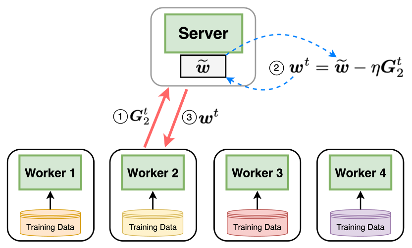
(a) Traditional ASGD

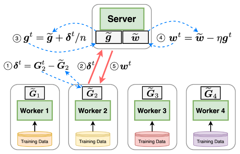
(b) DuDe-ASGD

Figure 1: Illustration of traditional ASGD and the proposed DuDe-ASGD. Suppose that worker 2 contributes to the server’s model update in iteration $t$. In traditional ASGD algorithms, each worker directly sends the freshly computed stochastic gradient ${\bm{G}}^{t}_{2}=\nabla f_{2}(\bm{w}^{t-\tau_{2}(t)};\bm{\xi}_{2}^{t})$ to the server. While in DuDe-ASGD, each worker maintains a memory of the most recently evaluated stochastic gradient $\widetilde{\bm{G}}_{2}$ and sends the gradient difference $\bm{\delta}^{t}={\bm{G}}^{t}_{2}-\widetilde{\bm{G}}_{2}$.

4 Theoretical Analysis

This section delves into the theoretical underpinnings of convergence behaviors of DuDe-ASGD. For clarity in our discussion, we present the convergence analysis of Algorithm 1 in its fully asynchronous form. The technical results discussed herein can be readily adapted to the semi-asynchronous variant of DuDe-ASGD, with or without the implementation of mini-batching.

To proceed, we introduce the following standard assumptions that are essential in our analysis.

Assumption 1.

There exists $F^{*}>-\infty$ such that (s.t.) $F(\bm{w})\geq F^{*}$ for all $\bm{w}\in\mathbb{R}^{p}$.

Assumption 2.

$F$ is $L$-smooth, i.e., $F$ is continuously differentiable and there exists $L\geq 0$ s.t.

$$\|\nabla F(\bm{w})-\nabla F(\bm{w}^{\prime})\|_{2}\leq L\|\bm{w}-\bm{w}^{\prime}\|_{2},\leavevmode\nobreak\ \leavevmode\nobreak\ \forall\leavevmode\nobreak\ \bm{w},\bm{w}^{\prime}\in\mathbb{R}^{p}.$$

Assumption 3.

Let $\bm{w}^{r}$ and $\bm{w}^{s}$ with $s,r\geq 0$ be iterates generated by Algorithm 1, $\bm{\xi}_{i}^{t}\in\Xi_{i}$ with $i\in[n]$ and $t\geq 1$ be a data sample drawn from $\mathbb{P}_{i}$, and ${\cal F}_{s}$ be the sigma algebra generated by $\bm{w}^{1},\dots,\bm{w}^{s}$. If $r\leq s<t$, then

$$\mathbb{E}\left[\nabla f_{i}(\bm{w}^{r};\bm{\xi}_{i}^{t})\mid{\cal F}_{s}\right]=\nabla F_{i}(\bm{w}^{r}).$$ (5)

Assumption 3 specifies that the stochastic gradient estimate is unbiased. It is important to note that the iterate $\bm{w}^{r}$ may depend on $\bm{\xi}_{i}^{t}$ for different times $r$ and $t$, rendering $\nabla f_{i}(\bm{w}^{r};\bm{\xi}_{i}^{t})$ a potentially biased estimate of $\nabla F_{i}(\bm{w}^{r})$. To maintain the unbiasedness as defined in equation (5), it is critical to ensure that $r\leq s<t$. This condition guarantees that ${\cal F}_{s}$ encompasses all information present in $\bm{w}^{r}$ and that $\bm{\xi}_{i}^{t}$ is independent of ${\cal F}_{s}$. Furthermore, we impose upper bounds on both the conditional variance of stochastic gradients:

Assumption 4.

Let $\bm{w}^{r}$ and $\bm{w}^{s}$ with $s,r\geq 0$ be iterates generated by Algorithm 1, $\bm{\xi}_{i}^{t}\in\Xi_{i}$ with $i\in[n]$ and $t\geq 1$ be a data sample drawn from $\mathbb{P}_{i}$, and ${\cal F}_{s}$ be the sigma algebra generated by $\bm{w}^{1},\dots,\bm{w}^{s}$. If $r\leq s<t$, then there exists a constant $\sigma\geq 0$ s.t.

$$\mathbb{E}\left[\|\nabla f_{i}(\bm{w}^{r};\bm{\xi}_{i}^{t})-\nabla F_{i}(\bm{w}^{r})\|_{2}^{2}\mid{\cal F}_{s}\right]\leq\sigma^{2}.$$

We further assume that each worker contributes to the server’s updates within a bounded number of global iterations, encapsulated by the following assumption regarding the maximum delay of model parameters:

Assumption 5.

There exists $\tau_{\max}\geq 1$ s.t. $\tau_{i}(t)\leq\tau_{\max}$ for all $i\in[n]$ in Algorithm 1.

When $\tau_{\max}=1$, indicating that all the models within $\bm{g}^{t}$ used in iteration (3) is up-to-date, Algorithm 1 simplifies to synchronous SGD. In the context of semi-asynchronous DuDe-ASGD where $|\mathcal{C}_{t}|=c\in[n]$ for all $t\geq 1$, we use $\tau_{\max}^{(c)}$ to denote the maximum model delay. Then, the relationship between $\tau_{\max}$ and $\tau_{\max}^{(c)}$ is characterized by $\tau_{\max}^{(c)}=\tau_{\max}/c$ (Nguyen et al., 2022, Appendix A). This formula signifies that the maximum model delay decreases proportionally to the number of workers the server waits for in each iteration. The technical results for fully asynchronous DuDe-ASGD (Algorithm 1) can be readily adapted to the semi-asynchronous variant by substituting $\tau_{\max}$ with $\tau_{\max}^{(c)}$ in our analysis.

4.1 Convergence Analysis of DuDe-ASGD

To study the convergence of DuDe-ASGD, we first observe that under Assumption 2, the following descent lemma holds:

$$\mathbb{E}[F(\bm{w}^{t})]-\mathbb{E}[F(\bm{w}^{t-1})]\leq \leavevmode\nobreak\ \mathbb{E}[\langle\nabla F(\bm{w}^{t-1}),\bm{w}^{t}-\bm{w}^{t-1}\rangle]+\frac{L}{2}\mathbb{E}\|\bm{w}^{t}-\bm{w}^{t-1}\|_{2}^{2}$$

$$= -\eta\mathbb{E}\langle\nabla F(\bm{w}^{t-1}),\bm{g}^{t}\rangle+\frac{L\eta^{2}}{2}\mathbb{E}\|\bm{g}^{t}\|_{2}^{2}.$$ (6)

Intuitively, both $\mathbb{E}\langle\nabla F(\bm{w}^{t-1}),\bm{g}^{t}\rangle$ and $\mathbb{E}\|\bm{g}^{t}\|_{2}^{2}$ can be regarded as biased estimates of $\|\nabla F(\bm{w}^{t-1})\|_{2}^{2}\geq 0$. Subsequently, selecting an appropriate step size $\eta$ can make the right-hand side of (6) negative, thereby ensuring a sufficient decrease in the expected function value in each iteration.

However, due to the dual delay properties of the information encapsulated in $\bm{g}^{t}$, handling the inner product term is not trivial. To describe the challenge, note that

$$\textstyle\langle\nabla F(\bm{w}^{t-1}),\bm{g}^{t}\rangle=\frac{1}{n}\sum_{i=1}^{n}\langle\nabla F(\bm{w}^{t-1}),\nabla f_{i}(\bm{w}^{t-\tau_{i}(t)};\bm{\xi}_{i}^{t-d_{i}(t)})\rangle.$$

We observe that $\bm{w}^{t-1}$ is a function of $\bm{\xi}_{i}^{t-d_{i}(t)}$ for $i\in[n]$ such that $d_{i}(t)\geq 1$. Consequently,

$$\mathbb{E}\langle\nabla F(\bm{w}^{t-1}),\nabla f_{i}(\bm{w}^{t-\tau_{i}(t)};\bm{\xi}_{i}^{t-d_{i}(t)})\rangle\neq\mathbb{E}\langle\nabla F(\bm{w}^{t-1}),\nabla F_{i}(\bm{w}^{t-\tau_{i}(t)})\rangle$$

and we can no longer obtain a simple expression for the expectation of the inner product. To address this challenge, our idea is to decompose the inner product into two terms:

$$\langle\nabla F(\bm{w}^{t-1}),\bm{g}^{t}\rangle=\langle\nabla F(\bm{w}^{[t-\tau_{\max}]_{+}}),\bm{g}^{t}\rangle+\langle\nabla F(\bm{w}^{t-1})-\nabla F(\bm{w}^{[t-\tau_{\max}]_{+}}),\bm{g}^{t}\rangle,$$ (7)

where $[x]_{+}\coloneqq\max\{x,0\}$ for $x\in\mathbb{R}$. Then utilizing Assumption 5 and considering the expectation conditioned on the most outdated model, we have the desired property:

$$\textstyle\mathbb{E}\left\langle\nabla F(\bm{w}^{[t-\tau_{\max}]_{+}}),\bm{g}^{t}\right\rangle=\frac{1}{n}\sum_{i=1}^{n}\mathbb{E}\langle\nabla F(\bm{w}^{[t-\tau_{\max}]_{+}}),\nabla F_{i}(\bm{w}^{t-\tau_{i}(t)})\rangle$$

Through carefully controlling the second error term, we arrive at the following lower bound on (7):

Proposition 1.

Suppose that Assumptions 2–5 hold. If the stepsize satisfies $\eta\leq\frac{1}{16L\tau_{\max}}$, then it holds for all $t\geq 1$ that

$$\mathbb{E}\langle\nabla F(\bm{w}^{t-1}),\bm{g}^{t}\rangle\geq\frac{1}{8}\mathbb{E}\|\nabla F(\bm{w}^{t-1})\|_{2}^{2}-2L\tau_{\max}\eta\sum_{s=1+[t-\tau_{\max}]_{+}}^{t}\mathbb{E}\|\nabla F(\bm{w}^{s-1})\|_{2}^{2}$$

$$\qquad\qquad\quad-3L\tau_{\max}\eta\frac{\sigma^{2}}{n}-6L^{2}\tau_{\max}\eta^{2}\sum_{s=1+[t-\tau_{\max}]_{+}}^{t}\mathbb{E}\left\|\frac{1}{n}\sum_{j=1}^{n}\nabla F_{j}(\bm{w}^{s-\tau_{j}(s)})\right\|_{2}^{2}.$$

The proof of Proposition 1 is deferred to Appendix B.2. Equipped with this, we finally establish the convergence rate of DuDe-ASGD by choosing proper step size $\eta$, as stated in the following theorem:

Theorem 1.

Suppose that Assumptions 1–5 hold. Let $\{\bm{w}^{t}\}_{t=1}^{T}$ be the sequence generated by Algorithm 1 and the step size be $\eta=\frac{1}{2}\sqrt{\frac{n\Delta}{L\sigma^{2}\tau_{\max}T}}$ with $\Delta\coloneqq F(\bm{w}^{0})-F^{*}$. Then, for $T\geq\frac{1024L\Delta n\tau_{\max}}{\sigma^{2}}$, it holds that

$$\frac{1}{T}\sum_{t=1}^{T}\mathbb{E}\|\nabla F(\bm{w}^{t-1})\|_{2}^{2}\leq 128\sqrt{\frac{L\Delta\sigma^{2}\tau_{\max}}{nT}}+\frac{128(L\Delta)^{3/2}\sqrt{n\tau_{\max}}}{\sigma T^{3/2}}.$$

The proof of Theorem 1 is deferred to Appendix B.3. Theorem 1 demonstrates that DuDe-ASGD converges to a stationary point of Problem (1) at a rate of $\mathcal{O}\left(\sqrt{{L\Delta\sigma^{2}\tau_{\max}}/{nT}}\right)$ and the transient time required for convergence exhibits a moderate linear dependence on both the number of workers $n$ and the maximum model delay $\tau_{\max}$. Critically, the convergence rate of DuDe-ASGD is achieved without imposing any assumptions on upper bounds for data heterogeneity or the dissimilarity among individual functions $F_{i}$. This indicates that DuDe-ASGD is well-suited for distributed environments with highly heterogeneous data. For sufficiently small $\epsilon>0$, we can deduce that after acquiring

$$\mathcal{O}\left(\frac{L\Delta\sigma^{2}\tau_{\max}}{n\epsilon^{2}}\right)\leavevmode\nobreak\ \leavevmode\nobreak\ \text{samples},$$ (8)

the iterates produced by Algorithm 1 satisfies $\frac{1}{T}\sum_{t=1}^{T}\mathbb{E}\|\nabla F(\bm{w}^{t-1})\|_{2}^{2}\leq\epsilon$. This sample complexity aligns closely with the theoretical lower bound for finding $\epsilon$-stationary points using stochastic first-order methods (Arjevani et al., 2023):

Corollary 1.

Provided that each worker contributes to the server’s updates just once every $n$ iterations, which implies that $\tau_{\max}=n$, then the sample complexity (8) of Algorithm 1 is minimax optimal.

4.2 Comparisons with Prior Works

We compare the theoretical performance of DuDe-ASGD with several representative distributed SGD-based algorithms as detailed in Table 1.

Aggregation-Based Algorithms. Representative SGD-based algorithms that employ full aggregation strategies include sIAG (Wang et al., 2023a) and MIFA (Gu et al., 2021), both of which operate synchronously. The analysis of sIAG is applicable only to strongly convex objectives. The convergence rate of MIFA is established based on the Lipschitz continuity of Hessians and boundedness of gradient noise, with the transient time $\Omega(n\tau_{\max}^{2})$ exhibiting a quadratic dependence on the maximum model delay. By contrast, our analysis is conducted under less restrictive conditions and achieves a reduced transient time. FedBuff (Nguyen et al., 2022), a notable semi-asynchronous federated learning algorithm, incorporates partial aggregation where only a subset of delayed local updates are considered during each global update. There has been several convergence analyses for FedBuff (Nguyen et al., 2022; Toghani and Uribe, 2022; Wang et al., 2023b), while they all assume equal probability of worker contributions to the global update—an idealistic scenario that rarely holds in practice.

Asynchronous Algorithms. The ASGD algorithms (Mishchenko et al., 2022; Koloskova et al., 2022; Islamov et al., 2024) require bounded data heterogeneity—an assumption not necessary in our analysis for DuDe-ASGD. In addition, through employing the full aggregation technique, the dominant term $\sqrt{1/nT}$ in the convergence rate of DuDe-ASGD suggests a linear speedup relative to the number of workers $n$, a feature not achieved in prior ASGD variants.

Table 1: Convergence rates of representative distributed SGD-based algorithms for solving smooth nonconvex objectives with heterogeneous data. (Shorthand notation: Async. = Asynchronous, Agg. = Aggregation-based, Add. Assump. = Additional assumptions aside from Assumptions 1–4, BDH = Bounded Data Heterogeneity, BN = Bounded Noise, LH = Lipschitz Hessian, UWP = Uniform Worker Participation, BG = Bounded Gradients)

Algorithms	Async.?	Agg.?	Convergence Rates	Add. Assump.
Synchronous SGD (Khaled and Richtárik, 2023)	No	Yes	$\displaystyle\mathcal{O}\left(\sqrt{\frac{\sigma^{2}}{nT}}+\frac{1}{T}\right)$	–
MIFA (Gu et al., 2021)	No	Yes	$\displaystyle\mathcal{O}\left(\sqrt{\frac{1+\tau_{\operatorname{avg}}}{nKT}}\sigma^{2}+\frac{nK\sigma\tau_{\max}{\color[rgb]{1,0,1}\zeta}+\sigma^{2}\tau_{\max}{\color[rgb]{1,0,1}\delta\rho}}{T}\right)$	BDH, BN, LH
FedBuff (Nguyen et al., 2022)	Semi	Partial	$\displaystyle\mathcal{O}\left(\frac{\sigma^{2}+K{\color[rgb]{1,0,1}\zeta^{2}}}{\sqrt{mKT}}+\frac{K\tau_{\operatorname{avg}}\tau_{\max}{\color[rgb]{1,0,1}\zeta^{2}}+\tau_{\max}\sigma^{2}}{T}\right)$	BDH, UWP
Vanilla ASGD (Mishchenko et al., 2022)	Yes	No	$\displaystyle\mathcal{O}\left(\sqrt{\frac{\sigma^{2}}{T}}+\frac{n}{T}+{\color[rgb]{1,0,1}\zeta_{\max}^{2}}\right)$	BDH
Uniform ASGD (Koloskova et al., 2022)	Yes	No	$\displaystyle\mathcal{O}\left(\sqrt{\frac{\sigma^{2}+{\color[rgb]{1,0,1}\zeta^{2}}}{T}}+\frac{\sqrt[3]{\tau_{\operatorname{avg}}\frac{1}{n}\sum_{i=1}^{n}\tau_{\operatorname{avg}}^{i}{\color[rgb]{1,0,1}\zeta_{i}^{2}}}}{T^{2/3}}\right)$	BDH
Shuffled ASGD (Islamov et al., 2024)	Yes	No	$\displaystyle\mathcal{O}\left(\sqrt{\frac{\sigma^{2}}{T}}+\frac{(\sqrt{n}{\color[rgb]{1,0,1}\zeta})^{2/3}+(n{\color[rgb]{1,0,1}G})^{2/3}}{T^{2/3}}+\frac{n}{T}\right)$	BDH, BG
DuDe-ASGD (This Paper)	Yes	Yes	$\displaystyle\mathcal{O}\left(\sqrt{\frac{\sigma^{2}\tau_{\max}}{nT}}+\frac{\sqrt{n\tau_{\max}}}{\sigma T^{3/2}}\right)$	–

5 Numerical Experiments

Experiment Setup. We simulate a distributed system comprising $n$ workers. To model the hardware variations across different workers, we employ the fixed-computation-speed model described in (Mishchenko et al., 2022). Specifically, each worker $i$ consistently takes fixed units of time, $s_{i}$, to compute a stochastic gradient. For each $i\in[n]$, $s_{i}$ is drawn from the truncated normal distribution $\mathcal{TN}(\mu,\texttt{std})$ with a mean $\mu=1$ and standard deviation $\texttt{std}=1$ and $5$, ensuring all time values are greater than $0$. A higher std indicates more significant hardware variation, leading to a greater maximum delay in the models during the training process. Furthermore, we assume that the communication time between the server and workers, as well as the server’s computation time for global updates, are negligible. We implement DuDe-ASGD in its fully asynchronous form using mini-batching, along with other distributed SGD-based algorithms listed in Table 1. Each mini-batch comprises 64 samples, uniformly drawn from the local datasets allocated to the workers. We evaluate the performance of these algorithms using the CIFAR-10 image dataset (Krizhevsky et al., 2009) by training a convolutional neural network with two convolutional layers for image classification. Following the approach described in Yurochkin et al. (2019), we allocate the dataset to the workers based on the Dirichlet distribution with concentration parameter $\alpha$. A lower $\alpha$ results in greater data heterogeneity among the workers. The step sizes for the algorithms under comparison are selected from the set $\{0.001,0.005,0.01\}$, based on which they achieve the fastest convergence. We implement all algorithms in PyTorch and run experiments on NVIDIA RTX A5000 GPUs.

Numerical Results. Each experiment is independently repeated three times using different random seeds, and the mean and standard deviation of the numerical performance for a configuration of $n=10$ workers are shown in Figure 2. In scenarios of high data heterogeneity, specifically $\alpha=0.1$, DuDe-ASGD demonstrates superior performance by achieving the fastest convergence rate in training loss and the highest test accuracy. Additionally, DuDe-ASGD maintains consistent performance even as the computation speeds of the workers vary significantly, as indicated by an increasing std, indicating its robustness to hardware variations. On the other hand, under conditions of low data heterogeneity, where $\alpha=0.5$, the performance of DuDe-ASGD aligns closely with that of vanilla ASGD. This similarity supports the theoretical convergence rate of vanilla ASGD, which includes an additive $\zeta_{\max}^{2}$ term that becomes less significant as $\alpha$ increases. The convergence rate of synchronous SGD is theoretically invariant across different levels of data heterogeneity. However, its practical runtime performance suffers from the slowest worker, particularly as std increases. Furthermore, the Uniform ASGD does not deliver satisfactory outcomes, potentially because the repeated sampling of a slow worker before it completes its task can impair performance.

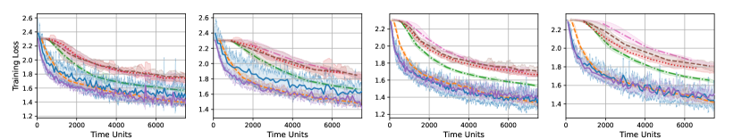
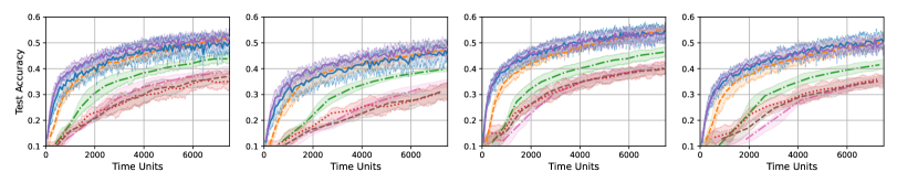
Figure 2: Convergence curves displaying training losses and test accuracies over time with $n=10$ workers. (1st column: $\alpha=0.1,\texttt{std}=1$; 2nd column: $\alpha=0.1,\texttt{std}=5$; 3rd column: $\alpha=0.5,\texttt{std}=1$; 4th column: $\alpha=0.5,\texttt{std}=5$)

6 Conclusion

This paper introduces the dual-delayed asynchronous SGD (DuDe-ASGD), a novel approach to distributed machine learning that effectively counteracts the challenges posed by data heterogeneity across workers. By leveraging an asynchronous mechanism that utilizes stale gradients from all workers, DuDe-ASGD not only alleviates synchronization overheads but also balances the contributions of diverse worker datasets to the learning process. Our comprehensive theoretical analysis shows that DuDe-ASGD achieves near-minimax-optimal convergence rates for nonconvex problems, regardless of variations in data distribution across workers. This significant advancement highlights the robustness and efficiency of DuDe-ASGD in handling highly heterogeneous data scenarios, which are prevalent in modern distributed environments. Experiments on real-world datasets validate its superior runtime performance under high data heterogeneity in comparison to other leading distributed SGD-based algorithms, thereby confirming its potential as an effective tool for large-scale machine learning tasks.

Appendix A Additional Related Works

Other Variants of ASGD. While numerous variants of ASGD have been developed, they mostly address simpler scenarios with homogeneous data [Agarwal and Duchi, 2011, Lian et al., 2015, Feyzmahdavian et al., 2016, Leblond et al., 2018, Stich and Karimireddy, 2020, Arjevani et al., 2020, Dutta et al., 2021], where all workers operate on the same loss function and possess data with an identical probability distribution. In this setup, Problem (1) reduces to

$$\min_{\bm{w}\in\mathbb{R}^{p}}\leavevmode\nobreak\ \mathbb{E}_{\bm{\xi}\sim\mathbb{P}_{1}}\left[f_{1}(\bm{w};\bm{\xi})\right].$$

Another line of research explores ASGD for homogeneous data under the model parallelism setting [Recht et al., 2011, De Sa et al., 2015, Mania et al., 2017], where each worker is solely responsible for updating a specific block of the model parameters independently, such as a distinct layer of a neural network. The assumption of data homogeneity is valid for shared-memory architectures; however, this assumption becomes highly idealistic in data-parallelism scenarios, where workers may hold significantly diverse local datasets, especially in applications such as Internet of Things, healthcare, and financial services [Li et al., 2020, Kairouz et al., 2021]. An independent line of works have also considered ASGD in decentralized networks [Lian et al., 2018, Even et al., 2024], contrasting with the more commonly studied centralized architectures, as depicted in Figure 1, that rely on a central server.

Asynchronous Federated Learning. Federated learning (FL) is an emerging distributed machine learning paradigm that pays particular attention to data privacy and heterogeneity. Asynchronous federated learning algorithms [Xie et al., 2019, Chen et al., 2020, Nguyen et al., 2022, Zakerinia et al., 2022, Wang et al., 2023b, Fraboni et al., 2023, Wang et al., 2024, Leconte et al., 2024b] share similarities with ASGD but typically include a local update strategy that potentially reduces the communication frequency between the server and workers. Among these works, FedBuff [Nguyen et al., 2022] serves as a representative algorithm where workers operate independently, and the server waits for a subset of workers $\mathcal{C}_{t}$ to submit their local updates in each global iteration. The local and global updates of FedBuff proceeds as follows:

$$\bm{w}_{i}^{\tau_{i}(t),k}=\bm{w}_{i}^{\tau_{i}(t),k-1}-\eta_{\ell}\nabla f_{i}(\bm{w}_{i}^{\tau_{i}(t),k-1};\bm{\xi}_{i}^{t,k}),\leavevmode\nobreak\ k=1,2,\dots,K,\leavevmode\nobreak\ i\in\mathcal{C}_{t},$$

$$\bm{w}^{t}=\bm{w}^{t-1}-\frac{\eta_{g}}{|\mathcal{C}_{t}|}\sum_{i\in\mathcal{C}_{t}}(\bm{w}_{i}^{\tau_{i}(t),0}-\bm{w}_{i}^{\tau_{i}(t),K}),\leavevmode\nobreak\ t=1,2,\dots,$$

where $\eta_{\ell}$ and $\eta_{g}$ are the local and global step sizes, respectively. This approach can be regarded as a semi-asynchronous algorithm designed to decrease communication frequency at the expense of increased waiting time. Nevertheless, the local update strategy in federated learning leads to the client drift phenomenon [Karimireddy et al., 2020, Sun et al., 2023], where local models at each worker tend to deviate from the global model. Therefore, asynchronous federated learning algorithms typically require either data heterogeneity or function dissimilarity to be bounded, so that local models remain closely aligned with the global model throughout the training process.

Incremental Aggregated Gradient (IAG)-Type Methods: The algorithmic concept of DuDe-ASGD is rooted in the well-established IAG methods [Blatt et al., 2007, Gurbuzbalaban et al., 2017, Vanli et al., 2018], which update the model parameters by using a combination of new and previously computed gradients. When solving Problem (1), the iterative formula of IAG can be expressed as:

$$\bm{w}^{t}=\bm{w}^{t-1}-\frac{\eta_{t}}{n}\sum_{i=1}^{n}\nabla F_{i}(\bm{w}^{t-\tau_{i}(t)}),\leavevmode\nobreak\ t=1,2,\dots,$$

where $\{\eta_{t}\}_{t\geq 1}$ are step sizes. IAG is suitable for asynchronous distributed implementations. SAG [Roux et al., 2012, Schmidt et al., 2017] and SAGA [Defazio et al., 2014] are randomized versions of IAG, where the index $i$ of the component function to be updated is selected at random in each iteration. Glasgow and Wootters [2022] developed ADSAGA, an extension of SAGA to the asynchronous setting, assuming a stochastic delay model and that the server is aware of the delay distribution. Nevertheless, these algorithms all assume that the exact gradients $\nabla F_{i}(\cdot)$ can be evaluated by each worker. This is a fundamental difference from our DuDe-ASGD, which relies solely on stochastic gradients $\nabla f_{i}(\cdot,\bm{\xi}_{i})$ for any $\bm{\xi}_{i}\in\Xi_{i}$.

Appendix B Proofs of Main Results

For random variables $P,Q$ and function $h$, we denote by

$$\mathbb{E}_{P}[h(P,Q)]\coloneqq\mathbb{E}[h(P,Q)\mid Q]$$

the conditional expectation with respect to $P$ while holding $Q$ constant.

B.1 Technical Lemmas

Lemma 1.

Suppose that Assumptions 3 and 4 hold. Then, it holds for all $t\geq 1$ that

$$\mathbb{E}\left\|\frac{1}{n}\sum_{i=1}^{n}\left(\nabla f_{i}(\bm{w}^{t-\tau_{i}(t)};\bm{\xi}_{i}^{t-d_{i}(t)})-\nabla F_{i}(\bm{w}^{t-\tau_{i}(t)})\right)\right\|_{2}^{2}\leq\frac{\sigma^{2}}{n}.$$

Proof.

Expanding the squared norm gives

$$\leavevmode\nobreak\ \mathbb{E}\left\|\frac{1}{n}\sum_{i=1}^{n}\left(\nabla f_{i}(\bm{w}^{t-\tau_{i}(t)};\bm{\xi}_{i}^{t-d_{i}(t)})-\nabla F_{i}(\bm{w}^{t-\tau_{i}(t)})\right)\right\|_{2}^{2}$$

$$= \leavevmode\nobreak\ \frac{1}{n^{2}}\sum_{i=1}^{n}\mathbb{E}\|\nabla f_{i}(\bm{w}^{t-\tau_{i}(t)};\bm{\xi}_{i}^{t-d_{i}(t)})-\nabla F_{i}(\bm{w}^{t-\tau_{i}(t)})\|_{2}^{2}$$

$$\leavevmode\nobreak\ +\frac{1}{n^{2}}\sum_{i\neq j}\underbrace{\mathbb{E}\left\langle\nabla f_{i}(\bm{w}^{t-\tau_{i}(t)};\bm{\xi}_{i}^{t-d_{i}(t)})-\nabla F_{i}(\bm{w}^{t-\tau_{i}(t)}),\nabla f_{j}(\bm{w}^{t-\tau_{j}(t)};\bm{\xi}_{j}^{t-d_{j}(t)})-\nabla F_{j}(\bm{w}^{t-\tau_{j}(t)})\right\rangle}_{Y_{ij}}$$ (9)

To simplify $Y_{ij}$ for $i,j\in[n]$ s.t. $i\neq j$, we assume without loss of generality that $d_{i}(t)\geq d_{j}(t)$. Then, $t-\tau_{i}(t)\leq t-d_{j}(t)$ and thus $\bm{\xi}_{j}^{t-d_{j}(t)}$ is independent of $\bm{w}^{t-\tau_{i}(t)}$. Hence, using the law of total expectation and Assumption 3, we have

$$Y_{ij}= \leavevmode\nobreak\ \mathbb{E}\left\langle\nabla f_{i}(\bm{w}^{t-\tau_{i}(t)};\bm{\xi}_{i}^{t-d_{i}(t)})-\nabla F_{i}(\bm{w}^{t-\tau_{i}(t)}),\nabla f_{j}(\bm{w}^{t-\tau_{j}(t)};\bm{\xi}_{j}^{t-d_{j}(t)})-\nabla F_{j}(\bm{w}^{t-\tau_{j}(t)})\right\rangle$$

$$= \leavevmode\nobreak\ \mathbb{E}\left[\mathbb{E}_{\bm{\xi}_{j}^{t-d_{j}(t)}\sim\mathbb{P}_{j}}\left\langle\nabla f_{i}(\bm{w}^{t-\tau_{i}(t)};\bm{\xi}_{i}^{t-d_{i}(t)})-\nabla F_{i}(\bm{w}^{t-\tau_{i}(t)}),\nabla f_{j}(\bm{w}^{t-\tau_{j}(t)};\bm{\xi}_{j}^{t-d_{j}(t)})-\nabla F_{j}(\bm{w}^{t-\tau_{j}(t)})\right\rangle\right]$$

$$= \leavevmode\nobreak\ \mathbb{E}\left[\left\langle\nabla f_{i}(\bm{w}^{t-\tau_{i}(t)};\bm{\xi}_{i}^{t-d_{i}(t)})-\nabla F_{i}(\bm{w}^{t-\tau_{i}(t)}),\mathbb{E}_{\bm{\xi}_{j}^{t-d_{j}(t)}}\left[\nabla f_{j}(\bm{w}^{t-\tau_{j}(t)};\bm{\xi}_{j}^{t-d_{j}(t)})-\nabla F_{j}(\bm{w}^{t-\tau_{j}(t)})\right]\right\rangle\right]$$

$$= \leavevmode\nobreak\ {0}.$$

Substituting this back into (9) gives

$$\leavevmode\nobreak\ \mathbb{E}\left\|\frac{1}{n}\sum_{i=1}^{n}\left(\nabla f_{i}(\bm{w}^{t-\tau_{i}(t)};\bm{\xi}_{i}^{t-d_{i}(t)})-\nabla F_{i}(\bm{w}^{t-\tau_{i}(t)})\right)\right\|_{2}^{2}$$

$$= \leavevmode\nobreak\ \frac{1}{n^{2}}\sum_{i=1}^{n}\mathbb{E}\|\nabla f_{i}(\bm{w}^{t-\tau_{i}(t)};\bm{\xi}_{i}^{t-d_{i}(t)})-\nabla F_{i}(\bm{w}^{t-\tau_{i}(t)})\|_{2}^{2}$$

$$= \leavevmode\nobreak\ \frac{1}{n^{2}}\sum_{i=1}^{n}\mathbb{E}\left[\mathbb{E}\left[\|\nabla f_{i}(\bm{w}^{t-\tau_{i}(t)};\bm{\xi}_{i}^{t-d_{i}(t)})-\nabla F_{i}(\bm{w}^{t-\tau_{i}(t)})\|_{2}^{2}\leavevmode\nobreak\ \middle|\leavevmode\nobreak\ \bm{w}^{t-\tau_{i}(t)}\right]\right]$$

$$\leq \leavevmode\nobreak\ \frac{\sigma^{2}}{n}.$$ (10)

where the second equality holds due to the law of total expectation and the inequality follows from Assumption 4. ∎

Lemma 2.

Suppose that Assumptions 3 and 4 hold. Then, it holds for all $i\in[n]$ and $t\geq 1$ that

$$\mathbb{E}\|\bm{w}^{t}-\bm{w}^{t-\tau_{i}(t)}\|_{2}^{2}\leq 2\tau_{\max}^{2}\eta^{2}\frac{\sigma^{2}}{n}+2\tau_{\max}\eta^{2}\sum_{s=1+[t-\tau_{\max}]_{+}}^{t}\mathbb{E}\left\|\frac{1}{n}\sum_{j=1}^{n}\nabla F_{j}(\bm{w}^{s-\tau_{j}(s)})\right\|_{2}^{2}.$$

Proof.

For all $i\in[n]$ and $t\geq 1$, it follows from the telescoping sum

$$\sum_{s=1+t-\tau_{i}(t)}^{t}\left(\bm{w}^{s}-\bm{w}^{s-1}\right)=\bm{w}^{t}-\bm{w}^{t-\tau_{i}(t)}$$

and the iterative formula (3) that

$$\mathbb{E}\|\bm{w}^{t}-\bm{w}^{t-\tau_{i}(t)}\|_{2}^{2}$$

$$=\leavevmode\nobreak\ \mathbb{E}\left\|\sum_{s=1+t-\tau_{i}(t)}^{t}\left(\bm{w}^{s}-\bm{w}^{s-1}\right)\right\|_{2}^{2}$$

$$=\leavevmode\nobreak\ \mathbb{E}\left\|\sum_{s=1+t-\tau_{i}(t)}^{t}\eta\bm{g}^{s}\right\|_{2}^{2}$$

$$=\leavevmode\nobreak\ \mathbb{E}\left\|\sum_{s=1+t-\tau_{i}(t)}^{t}\frac{\eta}{n}\sum_{j=1}^{n}\nabla f_{j}(\bm{w}^{s-\tau_{j}(s)};\bm{\xi}_{j}^{s-d_{j}(s)})\right\|_{2}^{2}$$

$$=\leavevmode\nobreak\ \frac{\eta^{2}}{n^{2}}\mathbb{E}\left\|\sum_{s=1+t-\tau_{i}(t)}^{t}\sum_{j=1}^{n}\left(\nabla f_{j}(\bm{w}^{s-\tau_{j}(s)};\bm{\xi}_{j}^{s-d_{j}(s)})-\nabla F_{j}(\bm{w}^{s-\tau_{j}(s)})+\nabla F_{j}(\bm{w}^{s-\tau_{j}(s)})\right)\right\|_{2}^{2}$$

$$\leq\leavevmode\nobreak\ \frac{2\eta^{2}}{n^{2}}\underbrace{\mathbb{E}\left\|\sum_{s=1+t-\tau_{i}(t)}^{t}\sum_{j=1}^{n}\left(\nabla f_{j}(\bm{w}^{s-\tau_{j}(s)};\bm{\xi}_{j}^{s-d_{j}(s)})-\nabla F_{j}(\bm{w}^{s-\tau_{j}(s)})\right)\right\|_{2}^{2}}_{\Phi_{1}}$$

$$+\frac{2\eta^{2}}{n^{2}}\underbrace{\mathbb{E}\left\|\sum_{s=1+t-\tau_{i}(t)}^{t}\sum_{j=1}^{n}\nabla F_{j}(\bm{w}^{s-\tau_{j}(s)})\right\|_{2}^{2}}_{\Phi_{2}},$$ (11)

where the inequality uses the fact that $\|\bm{x}+\bm{y}\|_{2}^{2}\leq 2\|\bm{x}\|_{2}^{2}+2\|\bm{y}\|_{2}^{2}$ for vectors $\bm{x}$ and $\bm{y}$. Subsequently, we upper bound $\Phi_{1}$ and $\Phi_{2}$, respectively.

Upper bounding $Y_{1}$: Expanding $\Phi_{1}$, we have

$$\Phi_{1}=\sum_{s=1+t-\tau_{i}(t)}^{t}\mathbb{E}\left\|\sum_{j=1}^{n}\left(\nabla f_{j}(\bm{w}^{s-\tau_{j}(s)};\bm{\xi}_{i}^{s-d_{j}(s)})-\nabla F_{j}(\bm{w}^{s-\tau_{j}(s)})\right)\right\|_{2}^{2}$$

$$+\sum_{\begin{subarray}{c}s,s^{\prime}:s\neq s^{\prime},\\ 1+t-\tau_{i}(t)\leq s,s^{\prime}\leq t\end{subarray}}\underbrace{\mathbb{E}\left\langle\sum_{j=1}^{n}\left(\nabla f_{j}(\bm{w}^{s-\tau_{j}(s)};\bm{\xi}_{j}^{s-d_{j}(s)})-\nabla F_{j}(\bm{w}^{s-\tau_{j}(s)})\right),\sum_{j=1}^{n}\left(\nabla f_{j}(\bm{w}^{s^{\prime}-\tau_{j}(s^{\prime})};\bm{\xi}_{j}^{s^{\prime}-d_{j}(s^{\prime})})-\nabla F_{j}(\bm{w}^{s^{\prime}-\tau_{j}(s^{\prime})})\right)\right\rangle}_{Z^{ss^{\prime}}}.$$ (12)

Inspecting the inner product terms in (12), we note that for all $s,s^{\prime}\in[1+t-\tau_{i}(t),t]$ s.t. $s\neq s^{\prime}$,

$$Z^{ss^{\prime}}= \leavevmode\nobreak\ \mathbb{E}\left\langle\sum_{j=1}^{n}\left(\nabla f_{j}(\bm{w}^{s-\tau_{j}(s)};\bm{\xi}_{j}^{s-d_{j}(s)})-\nabla F_{j}(\bm{w}^{s-\tau_{j}(s)})\right),\sum_{j=1}^{n}\left(\nabla f_{j}(\bm{w}^{s^{\prime}-\tau_{j}(s^{\prime})};\bm{\xi}_{j}^{s^{\prime}-d_{j}(s^{\prime})})-\nabla F_{j}(\bm{w}^{s^{\prime}-\tau_{j}(s^{\prime})})\right)\right\rangle$$

$$= \leavevmode\nobreak\ \mathbb{E}\left[\sum_{i=1}^{n}\sum_{j=1}^{n}\left\langle\nabla f_{i}(\bm{w}^{s-\tau_{i}(s)};\bm{\xi}_{i}^{s-d_{i}(s)})-\nabla F_{i}(\bm{w}^{s-\tau_{i}(s)}),\nabla f_{j}(\bm{w}^{s^{\prime}-\tau_{j}(s^{\prime})};\bm{\xi}_{j}^{s^{\prime}-d_{j}(s^{\prime})})-\nabla F_{j}(\bm{w}^{s^{\prime}-\tau_{j}(s^{\prime})})\right\rangle\right]$$

$$= \leavevmode\nobreak\ \sum_{i=1}^{n}\sum_{j=1}^{n}\mathbb{E}\left\langle\nabla f_{i}(\bm{w}^{s-\tau_{i}(s)};\bm{\xi}_{i}^{s-d_{i}(s)})-\nabla F_{i}(\bm{w}^{s-\tau_{i}(s)}),\nabla f_{j}(\bm{w}^{s^{\prime}-\tau_{j}(s^{\prime})};\bm{\xi}_{j}^{s^{\prime}-d_{j}(s^{\prime})})-\nabla F_{j}(\bm{w}^{s^{\prime}-\tau_{j}(s^{\prime})})\right\rangle$$

$$= \leavevmode\nobreak\ \sum_{j=1}^{n}\mathbb{E}\left\langle\nabla f_{j}(\bm{w}^{s-\tau_{j}(s)};\bm{\xi}_{j}^{s-d_{j}(s)})-\nabla F_{j}(\bm{w}^{s-\tau_{j}(s)}),\nabla f_{j}(\bm{w}^{s^{\prime}-\tau_{j}(s^{\prime})};\bm{\xi}_{j}^{s^{\prime}-d_{j}(s^{\prime})})-\nabla F_{j}(\bm{w}^{s^{\prime}-\tau_{j}(s^{\prime})})\right\rangle$$

$$\leavevmode\nobreak\ +\sum_{i,j:i\neq j}\underbrace{\mathbb{E}\left\langle\nabla f_{i}(\bm{w}^{s-\tau_{i}(s)};\bm{\xi}_{i}^{s-d_{i}(s)})-\nabla F_{i}(\bm{w}^{s-\tau_{i}(s)}),\nabla f_{j}(\bm{w}^{s^{\prime}-\tau_{j}(s^{\prime})};\bm{\xi}_{j}^{s^{\prime}-d_{j}(s^{\prime})})-\nabla F_{j}(\bm{w}^{s^{\prime}-\tau_{j}(s^{\prime})})\right\rangle}_{Z^{ss^{\prime}}_{ij}}$$ (13)

To simplify $Z^{ss^{\prime}}_{ij}$ for all $i,j\in[n]$ and $i\neq j$, we assume with out loss of generality that $s-d_{i}(s)\geq s^{\prime}-d_{j}(s^{\prime})$. This, together with the fact that $d_{j}(s^{\prime})\leq\tau_{j}(s^{\prime})$ by (4), implies that $s-d_{i}(s)\geq s^{\prime}-\tau_{j}(s^{\prime})$. Thus, $\bm{\xi}_{j}^{s-d_{i}(s)}$ is independent of $\bm{w}^{s^{\prime}-d_{j}(s^{\prime})}$. Further using the law of total expectation and Assumption 3, we have

$$Z^{ss^{\prime}}_{ij}= \leavevmode\nobreak\ \mathbb{E}\left[\mathbb{E}_{\bm{\xi}_{i}^{s-d_{i}(s)}}\left\langle\nabla f_{i}(\bm{w}^{s-\tau_{i}(s)};\bm{\xi}_{j}^{s-d_{i}(s)})-\nabla F_{i}(\bm{w}^{s-\tau_{i}(s)}),\nabla f_{j}(\bm{w}^{s^{\prime}-\tau_{i}(s^{\prime})};\bm{\xi}_{j}^{s^{\prime}-d_{j}(s^{\prime})})-\nabla F_{j}(\bm{w}^{s^{\prime}-\tau_{i}(s^{\prime})})\right\rangle\right]$$

$$= \leavevmode\nobreak\ \mathbb{E}\left[\left\langle\mathbb{E}_{\bm{\xi}_{i}^{s-d_{i}(s)}}\left[\nabla f_{i}(\bm{w}^{s-\tau_{i}(s)};\bm{\xi}_{i}^{s-d_{i}(s)})-\nabla F_{i}(\bm{w}^{s-\tau_{i}(s)})\right],\nabla f_{j}(\bm{w}^{s^{\prime}-\tau_{i}(s^{\prime})};\bm{\xi}_{j}^{s^{\prime}-d_{j}(s^{\prime})})-\nabla F_{j}(\bm{w}^{s^{\prime}-\tau_{i}(s^{\prime})})\right\rangle\right]$$

$$= \leavevmode\nobreak\ 0$$

Substituting this back into (13) and using Assumption 4, we have

$$Z^{ss^{\prime}}= \leavevmode\nobreak\ \sum_{j=1}^{n}\mathbb{E}\left\langle\nabla f_{j}(\bm{w}^{s-\tau_{j}(s)};\bm{\xi}_{j}^{t-d_{j}(s)})-\nabla F_{j}(\bm{w}^{s-\tau_{j}(s)}),\nabla f_{j}(\bm{w}^{s^{\prime}-\tau_{i}(s^{\prime})};\bm{\xi}_{j}^{s^{\prime}-d_{j}(s^{\prime})})-\nabla F_{j}(\bm{w}^{s^{\prime}-\tau_{i}(s^{\prime})})\right\rangle$$

$$\leq \leavevmode\nobreak\ \frac{1}{2}\sum_{j=1}^{n}\mathbb{E}\|\nabla f_{j}(\bm{w}^{s-\tau_{j}(s)};\bm{\xi}_{j}^{t-d_{j}(s)})-\nabla F_{j}(\bm{w}^{s-\tau_{j}(s)})\|_{2}^{2}$$

$$\leavevmode\nobreak\ +\frac{1}{2}\sum_{j=1}^{n}\mathbb{E}\|\nabla f_{j}(\bm{w}^{s^{\prime}-\tau_{i}(s^{\prime})};\bm{\xi}_{j}^{s^{\prime}-d_{j}(s^{\prime})})-\nabla F_{j}(\bm{w}^{s^{\prime}-\tau_{i}(s^{\prime})})\|_{2}^{2}$$

$$\leq \leavevmode\nobreak\ n\sigma^{2}.$$

Plugging this back into (12) and using Lemma 1 yield

$$\Phi_{1} \leq\sum_{s=1+t-\tau_{i}(t)}^{t}n\sigma^{2}+\sum_{\begin{subarray}{c}s,s^{\prime}:s\neq s^{\prime},\\ 1+t-\tau_{i}(t)\leq s,s^{\prime}\leq t\end{subarray}}n\sigma^{2}$$

$$=\tau_{i}(t)n\sigma^{2}+(\tau_{i}(t)^{2}-\tau_{i}(t))n\sigma^{2}$$

$$=\tau_{i}(t)^{2}n\sigma^{2}$$

$$\leq n\tau_{\max}^{2}\sigma^{2}.$$ (14)

Upper bounding $\Phi_{2}$: Following the fact that $\|\sum_{i=1}^{m}\bm{x}_{i}\|_{2}^{2}\leq m\sum_{i=1}^{m}\|\bm{x}_{i}\|_{2}^{2}$ for vectors $\bm{x}_{1},\dots,\bm{x}_{m}$, we have

$$\Phi_{2} =\mathbb{E}\left\|\sum_{s=1+t-\tau_{i}(t)}^{t}\sum_{j=1}^{n}\nabla F_{j}(\bm{w}^{s-\tau_{j}(s)})\right\|_{2}^{2}$$

$$\leq\tau_{i}(t)\sum_{s=1+t-\tau_{i}(t)}^{t}\mathbb{E}\left\|\sum_{j=1}^{n}\nabla F_{j}(\bm{w}^{s-\tau_{j}(s)})\right\|_{2}^{2}.$$

$$\leq\tau_{\max}\sum_{s=1+[t-\tau_{\max}]_{+}}^{t}\mathbb{E}\left\|\sum_{j=1}^{n}\nabla F_{j}(\bm{w}^{s-\tau_{j}(s)})\right\|_{2}^{2}.$$ (15)

Substituting (14) and (15) back into (11) gives

$$\mathbb{E}\|\bm{w}^{t}-\bm{w}^{t-\tau_{i}(t)}\|_{2}^{2}\leq\frac{2\sigma^{2}}{n}\tau_{\max}^{2}\eta^{2}+2\tau_{\max}\eta^{2}\sum_{s=1+[t-\tau_{\max}]_{+}}^{t}\mathbb{E}\left\|\frac{1}{n}\sum_{j=1}^{n}\nabla F_{j}(\bm{w}^{s-\tau_{j}(s)})\right\|_{2}^{2},$$

as desired. ∎

Lemma 3.

Suppose that Assumptions 2–4 hold. Then, it holds for all $i\in[n]$ and $t\geq 1$ that

$$\mathbb{E}\|\bm{g}^{t}\|_{2}^{2}\leq \left(2+8L^{2}\tau_{\max}^{2}\eta^{2}\right)\frac{\sigma^{2}}{n}+4\mathbb{E}\|\nabla F(\bm{w}^{t-1})\|_{2}^{2}$$

$$+8L^{2}\tau_{\max}\eta^{2}\sum_{s=1+[t-\tau_{\max}]_{+}}^{t}\mathbb{E}\left\|\frac{1}{n}\sum_{j=1}^{n}\nabla F_{j}(\bm{w}^{s-\tau_{j}(s)})\right\|_{2}^{2}.$$

Proof.

Following the fact that $\|\bm{x}+\bm{y}\|_{2}^{2}\leq 2\|\bm{x}\|_{2}^{2}+2\|\bm{y}\|_{2}^{2}$ for vectors $\bm{x}$ and $\bm{y}$, we have

$$\leavevmode\nobreak\ \mathbb{E}\|\bm{g}^{t}\|_{2}^{2}$$

$$= \leavevmode\nobreak\ \mathbb{E}\left\|\frac{1}{n}\sum_{i=1}^{n}\nabla f_{i}(\bm{w}^{t-\tau_{i}(t)};\bm{\xi}_{i}^{t-d_{i}(t)})\right\|_{2}^{2}$$

$$= \leavevmode\nobreak\ \mathbb{E}\left\|\frac{1}{n}\sum_{i=1}^{n}\left(\nabla f_{i}(\bm{w}^{t-\tau_{i}(t)};\bm{\xi}_{i}^{t-d_{i}(t)})-\nabla F_{i}(\bm{w}^{t-\tau_{i}(t)})\right)+\frac{1}{n}\sum_{i=1}^{n}\nabla F_{i}(\bm{w}^{t-\tau_{i}(t)})\right\|_{2}^{2}$$

$$\leq \leavevmode\nobreak\ 2\mathbb{E}\left\|\frac{1}{n}\sum_{i=1}^{n}\left(\nabla f_{i}(\bm{w}^{t-\tau_{i}(t)};\bm{\xi}_{i}^{t-d_{i}(t)})-\nabla F_{i}(\bm{w}^{t-\tau_{i}(t)})\right)\right\|_{2}^{2}+2\mathbb{E}\left\|\frac{1}{n}\sum_{i=1}^{n}\nabla F_{i}(\bm{w}^{t-\tau_{i}(t)})\right\|_{2}^{2}$$

$$\leq \leavevmode\nobreak\ \frac{2\sigma^{2}}{n}+2\underbrace{\mathbb{E}\left\|\frac{1}{n}\sum_{i=1}^{n}\nabla F_{i}(\bm{w}^{t-\tau_{i}(t)})\right\|_{2}^{2}}_{\Psi}.$$ (16)

where the last inequality holds due to Lemma 1. It suffices to upper bound $\Psi$. We observe that

$$\Psi =\mathbb{E}\left\|\frac{1}{n}\sum_{i=1}^{n}\nabla F_{i}(\bm{w}^{t-\tau_{i}(t)})\right\|_{2}^{2}$$

$$=\mathbb{E}\left\|\frac{1}{n}\sum_{i=1}^{n}\left(\nabla F_{i}(\bm{w}^{t-\tau_{i}(t)})-\nabla F_{i}(\bm{w}^{t})\right)+\frac{1}{n}\sum_{i=1}^{n}\nabla F_{i}(\bm{w}^{t-1})\right\|_{2}^{2}$$

$$\leq 2\mathbb{E}\left\|\frac{1}{n}\sum_{i=1}^{n}\left(\nabla F_{i}(\bm{w}^{t-\tau_{i}(t)})-\nabla F_{i}(\bm{w}^{t})\right)\right\|_{2}^{2}+2\mathbb{E}\left\|\frac{1}{n}\sum_{i=1}^{n}\nabla F_{i}(\bm{w}^{t-1})\right\|_{2}^{2}$$

$$\leq\frac{2}{n}\sum_{i=1}^{n}\mathbb{E}\|\nabla F_{i}(\bm{w}^{t-\tau_{i}(t)})-\nabla F_{i}(\bm{w}^{t})\|_{2}^{2}+2\mathbb{E}\|\nabla F(\bm{w}^{t-1})\|_{2}^{2}$$

$$\leq\frac{2L^{2}}{n}\sum_{i=1}^{n}\mathbb{E}\|\bm{w}^{t-\tau_{i}(t)}-\bm{w}^{t}\|_{2}^{2}+2\mathbb{E}\|\nabla F(\bm{w}^{t-1})\|_{2}^{2},$$ (17)

where the second inequality uses the fact that $\|\sum_{i=1}^{m}\bm{x}_{i}\|_{2}^{2}\leq m\sum_{i=1}^{m}\|\bm{x}_{i}\|_{2}^{2}$ for vectors $\bm{x}_{1},\dots,\bm{x}_{m}$. Substituting Lemma 2 into (17) gives

$$\Psi \leq 2L^{2}\left(\frac{2\sigma^{2}}{n}\tau_{\max}^{2}\eta^{2}+2\tau_{\max}\eta^{2}\sum_{s=1+[t-\tau_{\max}]_{+}}^{t}\mathbb{E}\left\|\frac{1}{n}\sum_{j=1}^{n}\nabla F_{j}(\bm{w}^{s-\tau_{j}(s)})\right\|_{2}^{2}\right)+2\mathbb{E}\|\nabla F(\bm{w}^{t-1})\|_{2}^{2}$$

$$=\frac{4\sigma^{2}}{n}L^{2}\tau_{\max}^{2}\eta^{2}+4L^{2}\tau_{\max}\eta^{2}\sum_{s=1+[t-\tau_{\max}]_{+}}^{t}\mathbb{E}\left\|\frac{1}{n}\sum_{j=1}^{n}\nabla F_{j}(\bm{w}^{s-\tau_{j}(s)})\right\|_{2}^{2}+2\mathbb{E}\|\nabla F(\bm{w}^{t-1})\|_{2}^{2}.$$ (18)

Plugging (18) back into (16) gives

$$\mathbb{E}\|\bm{g}^{t}\|_{2}^{2}\leq \left(2+8L^{2}\tau_{\max}^{2}\eta^{2}\right)\frac{\sigma^{2}}{n}+4\mathbb{E}\|\nabla F(\bm{w}^{t-1})\|_{2}^{2}$$

$$+8L^{2}\tau_{\max}\eta^{2}\sum_{s=1+[t-\tau_{\max}]_{+}}^{t}\mathbb{E}\left\|\frac{1}{n}\sum_{j=1}^{n}\nabla F_{j}(\bm{w}^{s-\tau_{j}(s)})\right\|_{2}^{2},$$

as desired. ∎

B.2 Proof of Proposition 1

Proof.

We first decompose the inner product into two terms:

$$\mathbb{E}\langle\nabla F(\bm{w}^{t-1}),\bm{g}^{t}\rangle=\underbrace{\mathbb{E}\left\langle\nabla F(\bm{w}^{[t-\tau_{\max}]_{+}}),\bm{g}^{t}\right\rangle}_{A}+\underbrace{\mathbb{E}\left\langle\nabla F(\bm{w}^{t-1})-\nabla F(\bm{w}^{[t-\tau_{\max}]_{+}}),\bm{g}^{t}\right\rangle}_{B}.$$ (19)

Subsequently, we upper bound $A_{1}$ and $A_{2}$, respectively.

Lower bounding $A$: Since $d_{i}(t)\leq\tau_{i}(t)\leq\tau_{\max}$ for all $i\in[n]$, then $t-d_{i}(t)\geq t-\tau_{\max}$ for all $i\in[n]$, which implies that $\bm{\xi}_{1}^{t-d_{1}(t)},\dots,\bm{\xi}_{n}^{t-d_{n}(t)}$ are independent of $\bm{w}^{[t-\tau_{\max}]_{+}}$. Then, we have

$$A= \leavevmode\nobreak\ \mathbb{E}\left[\left\langle\nabla F(\bm{w}^{[t-\tau_{\max}]_{+}}),\bm{g}^{t}\right\rangle\right]$$

$$\stackrel{{\scriptstyle(a)}}{{=}} \leavevmode\nobreak\ \mathbb{E}\left[\mathbb{E}_{\bm{\xi}_{1}^{t-d_{1}(t)},\dots,\bm{\xi}_{n}^{t-d_{n}(t)}}\left[\left\langle\nabla F(\bm{w}^{[t-\tau_{\max}]_{+}}),\bm{g}^{t}\right\rangle\right]\right]$$

$$= \leavevmode\nobreak\ \mathbb{E}\left\langle\nabla F(\bm{w}^{[t-\tau_{\max}]_{+}}),\mathbb{E}_{\bm{\xi}_{i}^{t-d_{i}(t)}}\left[\frac{1}{n}\sum_{i=1}^{n}\nabla f_{i}(\bm{w}^{t-\tau_{i}(t)};\bm{\xi}_{i}^{t-d_{i}(t)})\right]\right\rangle$$

$$\stackrel{{\scriptstyle(b)}}{{=}} \leavevmode\nobreak\ \mathbb{E}\left\langle\nabla F(\bm{w}^{[t-\tau_{\max}]_{+}}),\frac{1}{n}\sum_{i=1}^{n}\nabla F_{i}(\bm{w}^{t-\tau_{i}(t)})\right\rangle$$

$$= \leavevmode\nobreak\ \underbrace{\mathbb{E}\left\langle\nabla F(\bm{w}^{[t-\tau_{\max}]_{+}})-\nabla F(\bm{w}^{t-1}),\frac{1}{n}\sum_{i=1}^{n}\nabla F_{i}(\bm{w}^{t-\tau_{i}(t)})\right\rangle}_{A_{1}}$$

$$+\underbrace{\mathbb{E}\left\langle\nabla F(\bm{w}^{t-1}),\frac{1}{n}\sum_{i=1}^{n}\nabla F_{i}(\bm{w}^{t-\tau_{i}(t)})\right\rangle}_{A_{2}},$$ (20)

where $(a)$ use the law of total expectation, and $(b)$ holds due to Assumption 3. Then, we lower bound $A_{1}$ as follows:

$$A_{1}= \leavevmode\nobreak\ \mathbb{E}\left\langle\nabla F(\bm{w}^{[t-\tau_{\max}]_{+}})-\nabla F(\bm{w}^{t-1}),\frac{1}{n}\sum_{i=1}^{n}\left(\nabla F_{i}(\bm{w}^{t-\tau_{i}(t)})-\nabla F_{i}(\bm{w}^{t-1})\right)\right\rangle$$

$$+\mathbb{E}\left\langle\nabla F(\bm{w}^{[t-\tau_{\max}]_{+}})-\nabla F(\bm{w}^{t-1}),\nabla F(\bm{w}^{t-1})\right\rangle$$

$$\geq -\frac{1}{2}\mathbb{E}\|\nabla F(\bm{w}^{[t-\tau_{\max}]_{+}})-\nabla F(\bm{w}^{t-1})\|_{2}^{2}-\frac{1}{2}\mathbb{E}\left\|\frac{1}{n}\sum_{i=1}^{n}\left(\nabla F_{i}(\bm{w}^{t-\tau_{i}(t)})-\nabla F_{i}(\bm{w}^{t-1})\right)\right\|_{2}^{2}$$

$$-\mathbb{E}\|\nabla F(\bm{w}^{[t-\tau_{\max}]_{+}})-\nabla F(\bm{w}^{t-1})\|_{2}^{2}-\frac{1}{4}\mathbb{E}\|\nabla F(\bm{w}^{t-1})\|_{2}^{2}$$

$$= -\frac{1}{4}\mathbb{E}\|\nabla F(\bm{w}^{t-1})\|_{2}^{2}-\frac{3}{2}\mathbb{E}\|\nabla F(\bm{w}^{[t-\tau_{\max}]_{+}})-\nabla F(\bm{w}^{t-1})\|_{2}^{2}$$

$$-\frac{1}{2}\mathbb{E}\left\|\frac{1}{n}\sum_{i=1}^{n}\left(\nabla F_{i}(\bm{w}^{t-\tau_{i}(t)})-\nabla F_{i}(\bm{w}^{t-1})\right)\right\|_{2}^{2},$$ (21)

where the inequality uses the fact that $\langle\bm{x},\bm{y}\rangle\geq-\frac{1}{2}\|\bm{x}\|_{2}^{2}-\frac{1}{2}\|\bm{y}\|_{2}^{2}$ and $\langle\bm{x},\bm{y}\rangle\geq-\|\bm{x}\|_{2}^{2}-\frac{1}{4}\|\bm{y}\|_{2}^{2}$ for vectors $\bm{x}$ and $\bm{y}$. Using the identity $\langle\bm{x},\bm{y}\rangle=\frac{1}{2}\|\bm{x}\|_{2}^{2}+\frac{1}{2}\|\bm{y}\|_{2}^{2}-\frac{1}{2}\|\bm{x}-\bm{y}\|_{2}^{2}$ for vectors $\bm{x}$ and $\bm{y}$, we can express $A_{2}$ as

$$A_{2}= \leavevmode\nobreak\ \frac{1}{2}\mathbb{E}\|\nabla F(\bm{w}^{t-1})\|_{2}^{2}+\frac{1}{2}\mathbb{E}\left\|\frac{1}{n}\sum_{i=1}^{n}\nabla F_{i}(\bm{w}^{t-\tau_{i}(t)})\right\|_{2}^{2}$$

$$-\frac{1}{2}\mathbb{E}\left\|\nabla F(\bm{w}^{t-1})-\frac{1}{n}\sum_{i=1}^{n}\nabla F_{i}(\bm{w}^{t-\tau_{i}(t)})\right\|_{2}^{2}.$$ (22)

Putting (21) and (22) back into (20) gives

$$A\geq \leavevmode\nobreak\ \frac{1}{4}\mathbb{E}\|\nabla F(\bm{w}^{t-1})\|_{2}^{2}-\frac{3}{2}\mathbb{E}\|\nabla F(\bm{w}^{t-1})-\nabla F(\bm{w}^{[t-\tau_{\max}]_{+}})\|_{2}^{2}$$

$$-\mathbb{E}\left\|\frac{1}{n}\sum_{i=1}^{n}\left(\nabla F_{i}(\bm{w}^{t-1})-\nabla F_{i}(\bm{w}^{t-\tau_{i}(t)})\right)\right\|_{2}^{2}+\frac{1}{2}\mathbb{E}\left\|\frac{1}{n}\sum_{i=1}^{n}\nabla F_{i}(\bm{w}^{t-\tau_{i}(t)})\right\|_{2}^{2}$$

$$\stackrel{{\scriptstyle(a)}}{{=}} \leavevmode\nobreak\ \frac{1}{4}\mathbb{E}\|\nabla F(\bm{w}^{t-1})\|_{2}^{2}-\frac{3L^{2}}{2}\mathbb{E}\|\bm{w}^{t}-\bm{w}^{[t-\tau_{\max}]_{+}}\|_{2}^{2}$$

$$-\frac{L^{2}}{n}\sum_{i=1}^{n}\mathbb{E}\|\bm{w}^{t}-\bm{w}^{t-\tau_{i}(t)}\|_{2}^{2}+\frac{1}{2}\mathbb{E}\left\|\frac{1}{n}\sum_{i=1}^{n}\nabla F_{i}(\bm{w}^{t-\tau_{i}(t)})\right\|_{2}^{2}$$

$$\stackrel{{\scriptstyle(b)}}{{\geq}} \leavevmode\nobreak\ \frac{1}{4}\mathbb{E}\|\nabla F(\bm{w}^{t-1})\|_{2}^{2}+\frac{1}{2}\mathbb{E}\left\|\frac{1}{n}\sum_{i=1}^{n}\nabla F_{i}(\bm{w}^{t-\tau_{i}(t)})\right\|_{2}^{2}$$

$$-\frac{5L^{2}}{2}\left(2\tau_{\max}^{2}\eta^{2}\frac{\sigma^{2}}{n}+2\tau_{\max}\eta^{2}\sum_{s=1+[t-\tau_{\max}]_{+}}^{t}\mathbb{E}\left\|\frac{1}{n}\sum_{j=1}^{n}\nabla F_{j}(\bm{w}^{s-\tau_{j}(s)})\right\|_{2}^{2}\right)$$

$$= \leavevmode\nobreak\ \frac{1}{4}\mathbb{E}\|\nabla F(\bm{w}^{t-1})\|_{2}^{2}-5L^{2}\tau_{\max}^{2}\eta^{2}\frac{\sigma^{2}}{n}+\frac{1}{2}\mathbb{E}\left\|\frac{1}{n}\sum_{i=1}^{n}\nabla F_{i}(\bm{w}^{t-\tau_{i}(t)})\right\|_{2}^{2}$$

$$-5L^{2}\tau_{\max}\eta^{2}\sum_{s=1+[t-\tau_{\max}]_{+}}^{t}\mathbb{E}\left\|\frac{1}{n}\sum_{j=1}^{n}\nabla F_{j}(\bm{w}^{s-\tau_{j}(s)})\right\|_{2}^{2},$$ (23)

where $(a)$ uses Assumption 2 and $(b)$ uses Lemma 2.

Lower bounding $B$: We observe that

$$B =\mathbb{E}\left\langle\nabla F(\bm{w}^{t-1})-\nabla F(\bm{w}^{[t-\tau_{\max}]_{+}}),\bm{g}^{t}\right\rangle$$

$$\stackrel{{\scriptstyle(a)}}{{\geq}}-\mathbb{E}\left[\|\nabla F(\bm{w}^{t-1})-\nabla F(\bm{w}^{[t-\tau_{\max}]_{+}})\|_{2}\|\bm{g}^{t}\|_{2}\right]$$

$$\stackrel{{\scriptstyle(b)}}{{\geq}}-L\mathbb{E}\left[\|\bm{w}^{t}-\bm{w}^{[t-\tau_{\max}]_{+}}\|_{2}\|\bm{g}^{t}\|_{2}\right]$$

$$\stackrel{{\scriptstyle(c)}}{{\geq}}-L\mathbb{E}\left[\left\|\sum_{s=1+[t-\tau_{\max}]_{+}}^{t}\eta\bm{g}^{s}\right\|_{2}\|\bm{g}^{t}\|_{2}\right]$$

$$\stackrel{{\scriptstyle(d)}}{{\geq}}-L\mathbb{E}\left[\sum_{s=1+[t-\tau_{\max}]_{+}}^{t}\eta\|\bm{g}^{s}\|_{2}\|\bm{g}^{t}\|_{2}\right]$$

$$\stackrel{{\scriptstyle(e)}}{{\geq}}-L\eta\sum_{s=1+[t-\tau_{\max}]_{+}}^{t}\frac{1}{2}\left(\mathbb{E}\|\bm{g}^{s}\|_{2}^{2}+\mathbb{E}\|\bm{g}^{t}\|_{2}^{2}\right)$$

$$=-\frac{L\eta}{2}\sum_{s=1+[t-\tau_{\max}]_{+}}^{t}\mathbb{E}\|\bm{g}^{s}\|_{2}^{2}-\frac{L\eta}{2}\tau_{\max}\mathbb{E}\|\bm{g}^{t}\|_{2}^{2},$$ (24)

where $(a)$ follows from the Cauchy-Schwartz inequality, $(b)$ follows from Assumption 2, $(c)$ uses the telescoping sum $\bm{w}^{t}-\bm{w}^{[t-\tau_{\max}]_{+}}=\sum_{s=1+[t-\tau_{\max}]_{+}}^{t}\left(\bm{w}^{s}-\bm{w}^{s-1}\right)=\sum_{s=1+[t-\tau_{\max}]_{+}}^{t}\eta\bm{g}^{s}$, $(d)$ uses the triangle inequality, and $(e)$ is due to the Young’s inequality. Combining (24) with Lemma 3, we have

$$B\geq -\frac{L\eta}{2}\sum_{s=1+[t-\tau_{\max}]_{+}}^{t}\left(\left(2+8L^{2}\tau_{\max}^{2}\eta^{2}\right)\frac{\sigma^{2}}{n}+4\mathbb{E}\|\nabla F(\bm{w}^{s-1})\|_{2}^{2}\right.$$

$$\leavevmode\nobreak\ \left.\qquad\qquad\qquad\qquad\qquad+8L^{2}\tau_{\max}\eta^{2}\sum_{s^{\prime}=1+[s-\tau_{\max}]_{+}}^{s}\mathbb{E}\left\|\frac{1}{n}\sum_{j=1}^{n}\nabla F_{j}(\bm{w}^{s^{\prime}-\tau_{i}(s^{\prime})})\right\|_{2}^{2}\right)$$

$$-\frac{L\eta}{2}\tau_{\max}\left(\left(2+8L^{2}\tau_{\max}^{2}\eta^{2}\right)\frac{\sigma^{2}}{n}+4\mathbb{E}\|\nabla F(\bm{w}^{t-1})\|_{2}^{2}\right.$$

$$\left.\qquad\qquad\qquad\quad+8L^{2}\tau_{\max}\eta^{2}\sum_{s=1+[t-\tau_{\max}]_{+}}^{t}\mathbb{E}\left\|\frac{1}{n}\sum_{j=1}^{n}\nabla F_{j}(\bm{w}^{s-\tau_{j}(s)})\right\|_{2}^{2}\right)$$

$$= -(2L\tau_{\max}\eta+8L^{3}\tau_{\max}^{3}\eta^{3})\frac{\sigma^{2}}{n}-2L\eta\sum_{s=1+[t-\tau_{\max}]_{+}}^{t}\mathbb{E}\|\nabla F(\bm{w}^{s-1})\|_{2}^{2}-2L\tau_{\max}\eta\mathbb{E}\|\nabla F(\bm{w}^{t-1})\|_{2}^{2}$$

$$-4L^{3}\tau_{\max}\eta^{3}\sum_{s=1+[t-\tau_{\max}]_{+}}^{t}\sum_{s^{\prime}=1+[s-\tau_{\max}]_{+}}^{s}\mathbb{E}\left\|\frac{1}{n}\sum_{j=1}^{n}\nabla F_{j}(\bm{w}^{s^{\prime}-\tau_{i}(s^{\prime})})\right\|_{2}^{2}$$

$$-4L^{3}\tau_{\max}^{2}\eta^{3}\sum_{s=1+[t-\tau_{\max}]_{+}}^{t}\mathbb{E}\left\|\frac{1}{n}\sum_{j=1}^{n}\nabla F_{j}(\bm{w}^{s-\tau_{j}(s)})\right\|_{2}^{2}$$

$$\geq -(2L\tau_{\max}\eta+8L^{3}\tau_{\max}^{3}\eta^{3})\frac{\sigma^{2}}{n}-2L\eta\sum_{s=1+[t-\tau_{\max}]_{+}}^{t}\mathbb{E}\|\nabla F(\bm{w}^{s-1})\|_{2}^{2}-2L\tau_{\max}\eta\mathbb{E}\|\nabla F(\bm{w}^{t-1})\|_{2}^{2}$$

$$-8L^{3}\tau_{\max}^{2}\eta^{3}\sum_{s=1+[t-2\tau_{\max}]_{+}}^{t}\mathbb{E}\left\|\frac{1}{n}\sum_{j=1}^{n}\nabla F_{j}(\bm{w}^{s-\tau_{j}(s)})\right\|_{2}^{2},$$ (25)

where the last inequality uses the fact that $\sum_{s=1+[t-K]_{+}}^{t}\sum_{s^{\prime}=1+[s-K]_{+}}^{s}a_{s^{\prime}}\leq K\sum_{s=1+[t-2K]_{+}}^{t}a_{s}$ for $a_{1},\dots,a_{t}\geq 0$ and $K\geq 1$.

Substituting (23) and (25) into (19) and simplifying it, we have

$$\leavevmode\nobreak\ \mathbb{E}\langle\nabla F(\bm{w}^{t-1}),\bm{g}^{t}\rangle$$

$$\geq \left(\frac{1}{4}-2L\tau_{\max}\eta\right)\mathbb{E}\|\nabla F(\bm{w}^{t-1})\|_{2}^{2}-2L\eta\sum_{s=1+[t-\tau_{\max}]_{+}}^{t}\mathbb{E}\|\nabla F(\bm{w}^{s-1})\|_{2}^{2}$$

$$-(2L\tau_{\max}\eta+5L^{2}\tau_{\max}^{2}\eta^{2}+8L^{3}\tau_{\max}^{3}\eta^{3})\frac{\sigma^{2}}{n}+\frac{1}{2}\mathbb{E}\left\|\frac{1}{n}\sum_{i=1}^{n}\nabla F_{i}(\bm{w}^{t-\tau_{i}(t)})\right\|_{2}^{2}$$

$$-(5L^{2}\tau_{\max}\eta^{2}+8L^{3}\tau^{2}_{\max}\eta^{3})\sum_{s=1+[t-2\tau_{\max}]_{+}}^{t}\mathbb{E}\left\|\frac{1}{n}\sum_{j=1}^{n}\nabla F_{j}(\bm{w}^{s-\tau_{j}(s)})\right\|_{2}^{2}$$

$$\geq \leavevmode\nobreak\ \frac{1}{8}\mathbb{E}\|\nabla F(\bm{w}^{t-1})\|_{2}^{2}-2L\eta\sum_{s=1+[t-\tau_{\max}]_{+}}^{t}\mathbb{E}\|\nabla F(\bm{w}^{s-1})\|_{2}^{2}-3L\tau_{\max}\eta\frac{\sigma^{2}}{n}$$

$$\leavevmode\nobreak\ +\frac{1}{2}\mathbb{E}\left\|\frac{1}{n}\sum_{i=1}^{n}\nabla F_{i}(\bm{w}^{t-\tau_{i}(t)})\right\|_{2}^{2}-6L^{2}\tau_{\max}\eta^{2}\sum_{s=1+[t-2\tau_{\max}]_{+}}^{t}\mathbb{E}\left\|\frac{1}{n}\sum_{j=1}^{n}\nabla F_{j}(\bm{w}^{s-\tau_{j}(s)})\right\|_{2}^{2},$$

where the last inequality holds because the stepsize condition $\eta\leq 1/(16L\tau_{\max})$ implies the following:

$$\frac{1}{4}-2L\tau_{\max}\eta \geq\frac{1}{8},$$

$$2L\tau_{\max}\eta+5L^{2}\tau_{\max}^{2}\eta^{2}+8L^{3}\tau_{\max}^{3}\eta^{3} \leq 2L\tau_{\max}\eta+6L^{2}\tau_{\max}^{2}\eta^{2}\leq 3L\tau_{\max}\eta,$$

$$5L^{2}\tau_{\max}\eta^{2}+8L^{3}\tau_{\max}^{2}\eta^{3} \leq 6L^{2}\tau_{\max}\eta^{2}.$$

This completes the proof. ∎

B.3 Proof of Theorem 1

Proof.

Since $F$ is $L$-smooth, it follows from the descent lemma that

$$\mathbb{E}[F(\bm{w}^{t})]-\mathbb{E}[F(\bm{w}^{t-1})]\leq \leavevmode\nobreak\ \mathbb{E}[\langle\nabla F(\bm{w}^{t-1}),\bm{w}^{t}-\bm{w}^{t-1}\rangle]+\frac{L}{2}\mathbb{E}\|\bm{w}^{t}-\bm{w}^{t-1}\|_{2}^{2}$$

$$= -\eta\mathbb{E}\langle\nabla F(\bm{w}^{t-1}),\bm{g}^{t}\rangle+\frac{L\eta^{2}}{2}\mathbb{E}\|\bm{g}^{t}\|_{2}^{2}.$$

Applying Lemma 3 and Proposition 1, we obtain

$$\leavevmode\nobreak\ \mathbb{E}[F(\bm{w}^{t})]-\mathbb{E}[F(\bm{w}^{t-1})]$$

$$\leq -\frac{1}{8}\eta\mathbb{E}\|\nabla F(\bm{w}^{t-1})\|_{2}^{2}+2L\eta^{2}\sum_{s=1+[t-\tau_{\max}]_{+}}^{t}\mathbb{E}\|\nabla F(\bm{w}^{s-1})\|_{2}^{2}+3L\tau_{\max}\eta^{2}\frac{\sigma^{2}}{n}$$

$$-\frac{1}{2}\eta\mathbb{E}\left\|\frac{1}{n}\sum_{i=1}^{n}\nabla F_{i}(\bm{w}^{t-\tau_{i}(t)})\right\|_{2}^{2}+6L^{2}\tau_{\max}\eta^{3}\sum_{s=1+[t-2\tau_{\max}]_{+}}^{t}\mathbb{E}\left\|\frac{1}{n}\sum_{j=1}^{n}\nabla F_{j}(\bm{w}^{s-\tau_{j}(s)})\right\|_{2}^{2}$$

$$+\left(L\eta^{2}+4L^{3}\tau_{\max}^{2}\eta^{4}\right)\frac{\sigma^{2}}{n}+4L^{3}\tau_{\max}\eta^{4}\sum_{s=1+[t-\tau_{\max}]_{+}}^{t}\mathbb{E}\left\|\frac{1}{n}\sum_{j=1}^{n}\nabla F_{j}(\bm{w}^{s-\tau_{j}(s)})\right\|_{2}^{2}$$

$$+2L\eta^{2}\mathbb{E}\|\nabla F(\bm{w}^{t-1})\|_{2}^{2}$$

$$\leq -\left(\frac{1}{8}\eta-2L\eta^{2}\right)\mathbb{E}\|\nabla F(\bm{w}^{t-1})\|_{2}^{2}+2L\eta^{2}\sum_{s=1+[t-\tau_{\max}]_{+}}^{t}\mathbb{E}\|\nabla F(\bm{w}^{s-1})\|_{2}^{2}$$

$$+(L\eta^{2}+3L\tau_{\max}\eta^{2}+4L^{3}\tau_{\max}^{2}\eta^{4})\frac{\sigma^{2}}{n}-\frac{1}{2}\eta\mathbb{E}\left\|\frac{1}{n}\sum_{i=1}^{n}\nabla F_{i}(\bm{w}^{t-\tau_{i}(t)})\right\|_{2}^{2}$$

$$+(6L^{2}\tau_{\max}\eta^{3}+4L^{3}\tau_{\max}\eta^{4})\sum_{s=1+[t-2\tau_{\max}]_{+}}^{t}\mathbb{E}\left\|\frac{1}{n}\sum_{j=1}^{n}\nabla F_{j}(\bm{w}^{s-\tau_{j}(s)})\right\|_{2}^{2}$$

$$\leq -\frac{1}{16}\eta\mathbb{E}\|\nabla F(\bm{w}^{t-1})\|_{2}^{2}+2L\eta^{2}\sum_{s=1+[t-\tau_{\max}]_{+}}^{t}\mathbb{E}\|\nabla F(\bm{w}^{s-1})\|_{2}^{2}$$

$$+(4L\tau_{\max}\eta^{2}+4L^{3}\tau_{\max}^{2}\eta^{4})\frac{\sigma^{2}}{n}$$

$$-\frac{1}{2}\eta\mathbb{E}\left\|\frac{1}{n}\sum_{i=1}^{n}\nabla F_{i}(\bm{w}^{t-\tau_{i}(t)})\right\|_{2}^{2}+7L^{2}\tau_{\max}\eta^{3}\sum_{s=1+[t-2\tau_{\max}]_{+}}^{t}\mathbb{E}\left\|\frac{1}{n}\sum_{j=1}^{n}\nabla F_{j}(\bm{w}^{s-\tau_{j}(s)})\right\|_{2}^{2},$$ (26)

where the last inequality holds because $\tau_{\max}\geq 1\Rightarrow L\eta^{2}+3L\tau_{\max}\eta^{2}\leq 4L\tau_{\max}\eta$ and by requiring the following stepsize conditions:

$$\eta\leq\frac{1}{32L}\Longleftrightarrow \leavevmode\nobreak\ \frac{1}{8}\eta-2L\eta^{2}\geq\frac{1}{16}\eta,$$ (27)

$$\eta\leq\frac{1}{4L}\Longrightarrow \leavevmode\nobreak\ 6L^{2}\tau_{\max}\eta^{3}+4L^{3}\tau_{\max}\eta^{4}\leq 7L^{2}\tau_{\max}\eta^{3}.$$ (28)

Summing up both sides of inequality (26) for $t=1,\dots,T$ yields

$$\mathbb{E}[F(\bm{w}^{T})]-F(\bm{w}^{0})$$

$$\leq -\frac{1}{16}\eta\sum_{t=1}^{T}\mathbb{E}\|\nabla F(\bm{w}^{t-1})\|_{2}^{2}+2L\eta^{2}\sum_{t=1}^{T}\sum_{s=1+[t-\tau_{\max}]_{+}}^{t}\mathbb{E}\|\nabla F(\bm{w}^{s-1})\|_{2}^{2}$$

$$+\sum_{t=1}^{T}(4L\tau_{\max}\eta^{2}+4L^{3}\tau_{\max}^{2}\eta^{4})\frac{\sigma^{2}}{n}$$

$$-\frac{1}{2}\eta\sum_{t=1}^{T}\mathbb{E}\left\|\frac{1}{n}\sum_{j=1}^{n}\nabla F_{j}(\bm{w}^{t-\tau_{j}(t)})\right\|_{2}^{2}+7L^{2}\tau_{\max}\eta^{3}\sum_{t=1}^{T}\sum_{s=1+[t-2\tau_{\max}]_{+}}^{t}\mathbb{E}\left\|\frac{1}{n}\sum_{j=1}^{n}\nabla F_{j}(\bm{w}^{s-\tau_{j}(s)})\right\|_{2}^{2}$$

$$\leq -\frac{1}{16}\eta\sum_{t=1}^{T}\mathbb{E}\|\nabla F(\bm{w}^{t-1})\|_{2}^{2}+2L\tau_{\max}\eta^{2}\sum_{t=1}^{T}\mathbb{E}\|\nabla F(\bm{w}^{t-1})\|_{2}^{2}$$

$$+\sum_{t=1}^{T}(4L\tau_{\max}\eta^{2}+4L^{3}\tau_{\max}^{2}\eta^{4})\frac{\sigma^{2}}{n}$$

$$-\frac{1}{2}\eta\sum_{t=1}^{T}\mathbb{E}\left\|\frac{1}{n}\sum_{j=1}^{n}\nabla F_{j}(\bm{w}^{t-\tau_{j}(t)})\right\|_{2}^{2}+14L^{2}\tau_{\max}^{2}\eta^{3}\sum_{t=1}^{T}\mathbb{E}\left\|\frac{1}{n}\sum_{j=1}^{n}\nabla F_{j}(\bm{w}^{t-\tau_{j}(t)})\right\|_{2}^{2}$$

$$= -\left(\frac{1}{16}\eta-2L\tau_{\max}\eta^{2}\right)\sum_{t=1}^{T}\mathbb{E}\|\nabla F(\bm{w}^{t-1})\|_{2}^{2}+\sum_{t=1}^{T}(4L\tau_{\max}\eta^{2}+4L^{3}\tau_{\max}^{2}\eta^{4})\frac{\sigma^{2}}{n}$$

$$-\left(\frac{1}{2}\eta-14L^{2}\tau_{\max}^{2}\eta^{3}\right)\sum_{t=1}^{T}\mathbb{E}\left\|\frac{1}{n}\sum_{j=1}^{n}\nabla F_{j}(\bm{w}^{t-\tau_{j}(t)})\right\|_{2}^{2}$$

$$\leq -\frac{1}{32}\eta\sum_{t=1}^{T}\mathbb{E}\|\nabla F(\bm{w}^{t-1})\|_{2}^{2}+\sum_{t=1}^{T}(4L\tau_{\max}\eta^{2}+4L^{3}\tau_{\max}^{2}\eta^{4})\frac{\sigma^{2}}{n},$$ (29)

where the second inequality uses the fact that $\sum_{t=1}^{T}\sum_{s=1+[t-K]_{+}}^{t}a_{s}\leq K\sum_{t=1}^{T}a_{t}$ for $a_{1},\dots,a_{T}\geq 0$ and $K\geq 1$, and the last inequality holds by requiring the following stepsize conditions:

$$\eta\leq\frac{1}{64L\tau_{\max}} \Longleftrightarrow\frac{1}{16}\eta-2L\tau_{\max}\eta^{2}\geq\frac{1}{32}\eta,$$ (30)

$$\eta\leq\frac{1}{\sqrt{28}L\tau_{\max}} \Longleftrightarrow\frac{1}{2}\eta-14L^{2}\tau_{\max}^{2}\eta^{3}\geq 0.$$ (31)

Rearranging (29) and using Assumption 1, we obtain

$$\frac{1}{T}\sum_{t=1}^{T}\mathbb{E}\|\nabla F(\bm{w}^{t-1})\|_{2}^{2}\leq\frac{32(F(\bm{w}^{0})-F^{*})}{T\eta}+128L\tau_{\max}\eta\frac{\sigma^{2}}{n}+128L^{3}\tau_{\max}^{2}\eta^{3}\frac{\sigma^{2}}{n}.$$ (32)

It suffices to choose $\eta$ s.t. the right hind side of (32) can be minimized. To proceed, using the inequality $a+b\geq 2\sqrt{ab}$ for $a,b\geq 0$, we note that

$$\frac{32(F(\bm{w}^{0})-F^{*})}{T\eta}+128L\tau_{\max}\eta\frac{\sigma^{2}}{n}\geq 128\sqrt{\frac{L\sigma^{2}\tau_{\max}(F(\bm{w}^{0})-F^{*})}{nT}},$$

where the equality holds if and only if

$$\frac{32(F(\bm{w}^{0})-F^{*})}{T\eta}=128L\tau_{\max}\eta\frac{\sigma^{2}}{n}\Longleftrightarrow\eta=\frac{1}{2}\sqrt{\frac{n(F(\bm{w}^{0})-F^{*})}{L\sigma^{2}\tau_{\max}T}}.$$ (33)

Note that the stepsize conditions (27), (28), (30), and (31) are implied by $\eta\leq 1/(64L\tau_{\max})$. We take $\eta=\frac{1}{2}\sqrt{\frac{n(F(\bm{w}^{0})-F^{*})}{L\sigma^{2}\tau_{\max}T}}$, then the stepsize conditions can be satisfied when

$$\frac{1}{2}\sqrt{\frac{n(F(\bm{w}^{0})-F^{*})}{L\sigma^{2}\tau_{\max}T}}\leq\frac{1}{64L\tau_{\max}}\Longleftrightarrow T\geq\frac{1024L(F(\bm{w}^{0})-F^{*})n\tau_{\max}}{\sigma^{2}}.$$ (34)

Following from (32), when the number of iterations satisfies (34), we have

$$\frac{1}{T}\sum_{t=1}^{T}\mathbb{E}\|\nabla F(\bm{w}^{t-1})\|_{2}^{2}$$

$$\leq \leavevmode\nobreak\ 128\sqrt{\frac{L\sigma^{2}\tau_{\max}(F(\bm{w}^{0})-F^{*})}{nT}}+128L^{3}\tau_{\max}^{2}\left(\sqrt{\frac{n(F(\bm{w}^{0})-F^{*})}{4L\sigma^{2}\tau_{\max}T}}\right)^{3}\frac{\sigma^{2}}{n}$$

$$= \leavevmode\nobreak\ 128\sqrt{\frac{L\sigma^{2}\tau_{\max}(F(\bm{w}^{0})-F^{*})}{nT}}+\frac{128((F(\bm{w}^{0})-F^{*})L)^{3/2}\sqrt{n\tau_{\max}}}{\sigma T^{3/2}},$$ (35)

which completes the proof. ∎

Appendix C Additional Experimental Details and Numerical Results

Data Partitioning. Following the approaches adopted in many works [Yurochkin et al., 2019, Hsu et al., 2019, Li et al., 2022], we use Dirichlet distribution to split the CIFAR-10 dataset into $n$ subsets. The training set in CIFAR-10 consists of 50,000 images with 10 different classes. For each class $k\in[10]$, we generate a generate a vector $\bm{p}_{k}\in\mathbb{R}^{n}$ from the $n$-dimensional Dirichlet distribution with concentration parameter $\alpha$, whose probability density is given by

$$\text{Dir}_{n}(\bm{p}_{k};\alpha)\coloneqq\frac{1}{B(\alpha)}\prod_{i=1}^{n}p_{k,i}^{\alpha-1}.$$

Here, $B(\alpha)\coloneqq\frac{\prod_{i=1}^{n}\Gamma(\alpha)}{\Gamma(n\alpha)}$ is the Beta function, $\Gamma(\cdot)$ is the Gamma function, and $\bm{p}_{k}$ satisfies $p_{k,i}\in[0,1]$ and $\sum_{i=1}^{n}p_{k,i}=1$. After generating $\bm{p}_{1},\dots,\bm{p}_{10}$, each instance of class $k$ is assigned to client $i$ with probability $p_{k,i}$.

Numerical Results for $n=30$ Workers. We conduct experiments with a configuration of $n=30$ workers. Increasing the number of workers $n$ in the Dirichlet distribution with a given concentration parameter $\alpha$ tends to result in more balanced data partitioning. For our experiments, we select $\alpha=0.05$ and $0.1$ to observe the effects with $n=30$. Each experiment is independently conducted three times using different random seeds. We report the mean and standard deviation of the numerical performance for this configuration, as illustrated in Figure 3. We observe that DuDe-ASGD displays similar performance patterns to other algorithms, as previously shown in Figure 2, across different levels of data heterogeneity.

,

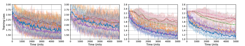
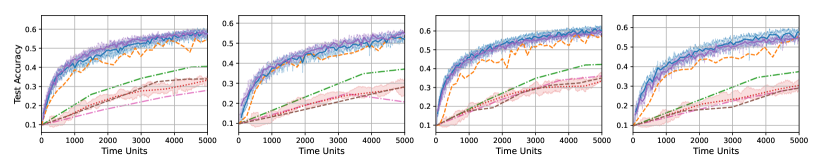
Figure 3: Convergence curves displaying training losses and test accuracies over time with $n=30$ workers. (1st column: $\alpha=0.05,\texttt{std}=1$; 2nd column: $\alpha=0.05,\texttt{std}=5$; 3rd column: $\alpha=0.1,\texttt{std}=1$; 4th column: $\alpha=0.1,\texttt{std}=5$)

References

• Agarwal and Duchi [2011] Alekh Agarwal and John C Duchi. Distributed delayed stochastic optimization. In Advances in Neural Information Processing Systems 24, 2011.
• Arjevani et al. [2020] Yossi Arjevani, Ohad Shamir, and Nathan Srebro. A tight convergence analysis for stochastic gradient descent with delayed updates. In Proceedings of the 31st International Conference on Algorithmic Learning Theory, pages 111–132. PMLR, 2020.
• Arjevani et al. [2023] Yossi Arjevani, Yair Carmon, John C Duchi, Dylan J Foster, Nathan Srebro, and Blake Woodworth. Lower bounds for non-convex stochastic optimization. Mathematical Programming, 199(1):165–214, 2023.
• Assran et al. [2020] Mahmoud Assran, Arda Aytekin, Hamid Reza Feyzmahdavian, Mikael Johansson, and Michael G Rabbat. Advances in asynchronous parallel and distributed optimization. Proceedings of the IEEE, 108(11):2013–2031, 2020.
• Avdiukhin and Kasiviswanathan [2021] Dmitrii Avdiukhin and Shiva Kasiviswanathan. Federated learning under arbitrary communication patterns. In Proceedings of the 38th International Conference on Machine Learning, pages 425–435. PMLR, 2021.
• Blatt et al. [2007] Doron Blatt, Alfred O Hero, and Hillel Gauchman. A convergent incremental gradient method with a constant step size. SIAM Journal on Optimization, 18(1):29–51, 2007.
• Chen et al. [2016] Jianmin Chen, Xinghao Pan, Rajat Monga, Samy Bengio, and Rafal Jozefowicz. Revisiting distributed synchronous SGD. arXiv preprint arXiv:1604.00981, 2016.
• Chen et al. [2020] Yujing Chen, Yue Ning, Martin Slawski, and Huzefa Rangwala. Asynchronous online federated learning for edge devices with non-IID data. In Proceedings of the 2020 IEEE International Conference on Big Data, pages 15–24. IEEE, 2020.
• Cotter et al. [2011] Andrew Cotter, Ohad Shamir, Nati Srebro, and Karthik Sridharan. Better mini-batch algorithms via accelerated gradient methods. In Advances in Neural Information Processing Systems 24, 2011.
• De Sa et al. [2015] Christopher M De Sa, Ce Zhang, Kunle Olukotun, and Christopher Ré. Taming the wild: A unified analysis of Hogwild-style algorithms. In Advances in Neural Information Processing Systems 28, 2015.
• Defazio et al. [2014] Aaron Defazio, Francis Bach, and Simon Lacoste-Julien. SAGA: A fast incremental gradient method with support for non-strongly convex composite objectives. In Advances in Neural Information Processing Systems 27, 2014.
• Dekel et al. [2012] Ofer Dekel, Ran Gilad-Bachrach, Ohad Shamir, and Lin Xiao. Optimal distributed online prediction using mini-batches. Journal of Machine Learning Research, 13(1), 2012.
• Dutta et al. [2021] Sanghamitra Dutta, Jianyu Wang, and Gauri Joshi. Slow and stale gradients can win the race. IEEE Journal on Selected Areas in Information Theory, 2(3):1012–1024, 2021.
• Even et al. [2024] Mathieu Even, Anastasia Koloskova, and Laurent Massoulié. Asynchronous SGD on graphs: A unified framework for asynchronous decentralized and federated optimization. In Proceedings of the 27th International Conference on Artificial Intelligence and Statistics, pages 64–72. PMLR, 2024.
• Feyzmahdavian et al. [2016] Hamid Reza Feyzmahdavian, Arda Aytekin, and Mikael Johansson. An asynchronous mini-batch algorithm for regularized stochastic optimization. IEEE Transactions on Automatic Control, 61(12):3740–3754, 2016.
• Fraboni et al. [2023] Yann Fraboni, Richard Vidal, Laetitia Kameni, and Marco Lorenzi. A general theory for federated optimization with asynchronous and heterogeneous clients updates. Journal of Machine Learning Research, 24(110):1–43, 2023.
• Gao et al. [2021] Hongchang Gao, Gang Wu, and Ryan Rossi. Provable distributed stochastic gradient descent with delayed updates. In Proceedings of the 2021 SIAM International Conference on Data Mining, pages 441–449. SIAM, 2021.
• Glasgow and Wootters [2022] Margalit R Glasgow and Mary Wootters. Asynchronous distributed optimization with stochastic delays. In Proceedings of the 25th International Conference on Artificial Intelligence and Statistics, pages 9247–9279. PMLR, 2022.
• Goyal et al. [2017] Priya Goyal, Piotr Dollár, Ross Girshick, Pieter Noordhuis, Lukasz Wesolowski, Aapo Kyrola, Andrew Tulloch, Yangqing Jia, and Kaiming He. Accurate, large minibatch SGD: Training ImageNet in 1 hour. arXiv preprint arXiv:1706.02677, 2017.
• Gu et al. [2021] Xinran Gu, Kaixuan Huang, Jingzhao Zhang, and Longbo Huang. Fast federated learning in the presence of arbitrary device unavailability. In Advances in Neural Information Processing Systems 34, pages 12052–12064, 2021.
• Gurbuzbalaban et al. [2017] Mert Gurbuzbalaban, Asuman Ozdaglar, and Pablo A Parrilo. On the convergence rate of incremental aggregated gradient algorithms. SIAM Journal on Optimization, 27(2):1035–1048, 2017.
• Hsu et al. [2019] Tzu-Ming Harry Hsu, Hang Qi, and Matthew Brown. Measuring the effects of non-identical data distribution for federated visual classification. arXiv preprint arXiv:1909.06335, 2019.
• Islamov et al. [2024] Rustem Islamov, Mher Safaryan, and Dan Alistarh. AsGrad: A sharp unified analysis of asynchronous-SGD algorithms. In Proceedings of the 27th International Conference on Artificial Intelligence and Statistics, pages 649–657. PMLR, 2024.
• Kairouz et al. [2021] Peter Kairouz, H Brendan McMahan, Brendan Avent, Aurélien Bellet, Mehdi Bennis, Arjun Nitin Bhagoji, Kallista Bonawitz, Zachary Charles, Graham Cormode, Rachel Cummings, et al. Advances and open problems in federated learning. Foundations and Trends® in Machine Learning, 14(1–2):1–210, 2021.
• Karimireddy et al. [2020] Sai Praneeth Karimireddy, Satyen Kale, Mehryar Mohri, Sashank Reddi, Sebastian Stich, and Ananda Theertha Suresh. Scaffold: Stochastic controlled averaging for federated learning. In Proceedings of the 37th International Conference on Machine Learning, pages 5132–5143. PMLR, 2020.
• Khaled and Richtárik [2023] Ahmed Khaled and Peter Richtárik. Better theory for SGD in the nonconvex world. Transactions on Machine Learning Research, 2023.
• Koloskova et al. [2022] Anastasiia Koloskova, Sebastian U Stich, and Martin Jaggi. Sharper convergence guarantees for asynchronous SGD for distributed and federated learning. In Advances in Neural Information Processing Systems 35, pages 17202–17215, 2022.
• Krizhevsky et al. [2009] Alex Krizhevsky, Geoffrey Hinton, et al. Learning multiple layers of features from tiny images. Technical report, University of Toronto, 2009. Available online: https://www.cs.utoronto.ca/~kriz/learning-features-2009-TR.pdf.
• Leblond et al. [2018] Rémi Leblond, Fabian Pedregosa, and Simon Lacoste-Julien. Improved asynchronous parallel optimization analysis for stochastic incremental methods. Journal of Machine Learning Research, 19(81):1–68, 2018.
• Leconte et al. [2024a] Louis Leconte, Matthieu Jonckheere, Sergey Samsonov, and Eric Moulines. Queuing dynamics of asynchronous federated learning. In Proceedings of the 27th International Conference on Artificial Intelligence and Statistics, pages 1711–1719. PMLR, 2024a.
• Leconte et al. [2024b] Louis Leconte, Eric Moulines, et al. FAVANO: Federated averaging with asynchronous nodes. In Proceedings of the 2024 IEEE International Conference on Acoustics, Speech and Signal Processing, pages 5665–5669. IEEE, 2024b.
• Li et al. [2022] Qinbin Li, Yiqun Diao, Quan Chen, and Bingsheng He. Federated learning on non-IID data silos: An experimental study. In Proceedings of the 2022 IEEE 38th International Conference on Data Engineering, pages 965–978. IEEE, 2022.
• Li et al. [2020] Tian Li, Anit Kumar Sahu, Ameet Talwalkar, and Virginia Smith. Federated learning: Challenges, methods, and future directions. IEEE Signal Processing Magazine, 37(3):50–60, 2020.
• Lian et al. [2015] Xiangru Lian, Yijun Huang, Yuncheng Li, and Ji Liu. Asynchronous parallel stochastic gradient for nonconvex optimization. In Advances in Neural Information Processing Systems 28, 2015.
• Lian et al. [2018] Xiangru Lian, Wei Zhang, Ce Zhang, and Ji Liu. Asynchronous decentralized parallel stochastic gradient descent. In Proceedings of the 37th International Conference on Machine Learning, pages 3043–3052. PMLR, 2018.
• Mania et al. [2017] Horia Mania, Xinghao Pan, Dimitris Papailiopoulos, Benjamin Recht, Kannan Ramchandran, and Michael I Jordan. Perturbed iterate analysis for asynchronous stochastic optimization. SIAM Journal on Optimization, 27(4):2202–2229, 2017.
• Mishchenko et al. [2022] Konstantin Mishchenko, Francis Bach, Mathieu Even, and Blake E Woodworth. Asynchronous SGD beats minibatch SGD under arbitrary delays. In Advances in Neural Information Processing Systems 35, pages 420–433, 2022.
• Nedić et al. [2001] Angelia Nedić, Dimitri P Bertsekas, and Vivek S Borkar. Distributed asynchronous incremental subgradient methods. Studies in Computational Mathematics, 8(C):381–407, 2001.
• Nguyen et al. [2022] John Nguyen, Kshitiz Malik, Hongyuan Zhan, Ashkan Yousefpour, Mike Rabbat, Mani Malek, and Dzmitry Huba. Federated learning with buffered asynchronous aggregation. In Proceedings of the 25th International Conference on Artificial Intelligence and Statistics, pages 3581–3607. PMLR, 2022.
• Recht et al. [2011] Benjamin Recht, Christopher Re, Stephen Wright, and Feng Niu. Hogwild!: A lock-free approach to parallelizing stochastic gradient descent. In Advances in Neural Information Processing Systems 24, 2011.
• Roux et al. [2012] Nicolas Roux, Mark Schmidt, and Francis Bach. A stochastic gradient method with an exponential convergence rate for finite training sets. In Advances in Neural Information Processing Systems 25, 2012.
• Schmidt et al. [2017] Mark Schmidt, Nicolas Le Roux, and Francis Bach. Minimizing finite sums with the stochastic average gradient. Mathematical Programming, 162:83–112, 2017.
• Stich and Karimireddy [2020] Sebastian U Stich and Sai Praneeth Karimireddy. The error-feedback framework: SGD with delayed gradients. Journal of Machine Learning Research, 21(237):1–36, 2020.
• Sun et al. [2023] Yuchang Sun, Yuyi Mao, and Jun Zhang. MimiC: Combating client dropouts in federated learning by mimicking central updates. IEEE Transactions on Mobile Computing, 2023.
• Toghani and Uribe [2022] Mohammad Taha Toghani and César A Uribe. Unbounded gradients in federated learning with buffered asynchronous aggregation. In Proceedings of the 2022 58th Annual Allerton Conference on Communication, Control, and Computing, pages 1–8. IEEE, 2022.
• Vanli et al. [2018] N Denizcan Vanli, Mert Gurbuzbalaban, and Asuman Ozdaglar. Global convergence rate of proximal incremental aggregated gradient methods. SIAM Journal on Optimization, 28(2):1282–1300, 2018.
• Verbraeken et al. [2020] Joost Verbraeken, Matthijs Wolting, Jonathan Katzy, Jeroen Kloppenburg, Tim Verbelen, and Jan S Rellermeyer. A survey on distributed machine learning. ACM Computing Surveys, 53(2):1–33, 2020.
• Wang et al. [2023a] Xiaolu Wang, Cheng Jin, Hoi-To Wai, and Yuantao Gu. Linear speedup of incremental aggregated gradient methods on streaming data. In Proceedings of the 2023 62nd IEEE Conference on Decision and Control, pages 4314–4319. IEEE, 2023a.
• Wang et al. [2024] Xiaolu Wang, Zijian Li, Shi Jin, and Jun Zhang. Achieving linear speedup in asynchronous federated learning with heterogeneous clients. arXiv preprint arXiv:2402.11198, 2024.
• Wang et al. [2023b] Yujia Wang, Yuanpu Cao, Jingcheng Wu, Ruoyu Chen, and Jinghui Chen. Tackling the data heterogeneity in asynchronous federated learning with cached update calibration. In Proceedings of the 12th International Conference on Learning Representations, 2023b.
• Xie et al. [2019] Cong Xie, Sanmi Koyejo, and Indranil Gupta. Asynchronous federated optimization. arXiv preprint arXiv:1903.03934, 2019.
• Yang et al. [2019] Qiang Yang, Yang Liu, Tianjian Chen, and Yongxin Tong. Federated machine learning: Concept and applications. ACM Transactions on Intelligent Systems and Technology, 10(2):1–19, 2019.
• Yurochkin et al. [2019] Mikhail Yurochkin, Mayank Agarwal, Soumya Ghosh, Kristjan Greenewald, Nghia Hoang, and Yasaman Khazaeni. Bayesian nonparametric federated learning of neural networks. In Proceedings of the 36th International Conference on Machine Learning, pages 7252–7261. PMLR, 2019.
• Zakerinia et al. [2022] Hossein Zakerinia, Shayan Talaei, Giorgi Nadiradze, and Dan Alistarh. QuAFL: Federated averaging can be both asynchronous and communication-efficient. arXiv preprint arXiv:2206.10032, 2022.
• Zhang et al. [2023] Feilong Zhang, Xianming Liu, Shiyi Lin, Gang Wu, Xiong Zhou, Junjun Jiang, and Xiangyang Ji. No one idles: Efficient heterogeneous federated learning with parallel edge and server computation. In Proceedings of the 40th International Conference on Machine Learning, pages 41399–41413. PMLR, 2023.