Distributed Riemannian Stochastic Gradient Tracking Algorithm on the Stiefel Manifold

Abstract

This paper focus on investigating the distributed Riemannian stochastic optimization problem on the Stiefel manifold for multi-agent systems, where all the agents work collaboratively to optimize a function modeled by the average of their expectation-valued local costs. Each agent only processes its own local cost function and communicate with neighboring agents to achieve optimal results while ensuring consensus. Since the local Riemannian gradient in stochastic regimes cannot be directly calculated, we will estimate the gradient by the average of a variable number of sampled gradient, which however brings about noise to the system. We then propose a distributed Riemannian stochastic optimization algorithm on the Stiefel manifold by combining the variable sample size gradient approximation method with the gradient tracking dynamic. It is worth noticing that the suitably chosen increasing sample size plays an important role in improving the algorithm efficiency, as it reduces the noise variance. In an expectation-valued sense, the iterates of all agents are proved to converge to a stationary point (or neighborhood) with fixed step sizes. We further establish the convergence rate of the iterates for the cases when the sample size is exponentially increasing, polynomial increasing, or a constant, respectively. Finally, numerical experiments are implemented to demonstrate the theoretical results.

1 Introduction

Distributed optimization has attracted much research attention in the past decades, motivated by the need to solve optimization problems over large-scale datasets or complex multi-agent systems. It is worth noticing that some of the problems have particular manifold constraints, e.g. decentralized spectral analysis [11, 12], dictionary learning [24], and deep neural networks with orthogonal constraint [32]. Therefore, solving distributed optimization problems on Riemannian manifold has also received significant research attention over the past few years [7, 9, 33, 16, 6, 34].

Let $\text{St}(n,r)$ denote the Stiefel manifold, and consider the function $f:\text{St}(n,r)\mapsto\mathbb{R}$. We focus on the following Riemannian stochastic optimization problem over connected networks:

$$\min f(X):=\frac{1}{N}\sum_{i=1}^{N}f_{i}(X),$$ (1)

$$s.t. X\in\mathcal{M}\triangleq\text{St}(n,r):=\{X\in\mathbb{R}^{n\times r}:X^{\top}X=I_{r}\},$$

where $I_{r}$ is the $r\times r$ identity matrix and the local cost function privately known by agent $i$ is an expectation-valued function defined as $f_{i}(X):=\mathbb{E}_{\xi_{i}}F_{i}(X,\xi_{i})$. Though each agent merely has its local information, it can interact with its neighbors through a connected graph $\mathcal{G}=(\mathcal{N},\mathcal{E})$ to collaboratively solve the problem (1). Here, $\mathcal{N}:=\{1,\dots,N\}$ denotes the index set including all agents, and $\mathcal{E}\subset\mathcal{N}\times\mathcal{N}$ denotes the set of all communication links. If $(i,j)\in\mathcal{E}$, then node $i$ can send information to node $j$. Problem (1) extends the distributed stochastic optimization problem in Euclidean space to the Stiefel manifold, which however is non-convex in Euclidean space. Next, we initiate a review of prior work.

1.1 Related Works

Stochastic distributed optimization has particular research interests among various distributed optimization frameworks, where the local cost functions are the expectation of functions with stochastic variables. Since the expectation-valued function has no closed-form, it could be prohibitive or costly to compute the exact gradient in big-data scenarios. Stochastic approximation (SA), originated from Robbins and Monro in the 1950s [26], is a commonly used method in algorithm design. The main idea of SA is to utilize a stochastic gradient to approximate the exact gradient. As such, stochastic gradient descent (SGD) has received extensive attention since it is practical and performs well in large-scale learning [4]. In recent years, distributed stochastic optimization in the Euclidean space has been widely studied where all the agents find the optimal solution cooperatively, such as [19, 30, 22, 28, 14, 2].

However, it is unable to solve problem (1) directly using the aforementioned studies since the Stiefel manifold constraint lacks of convexity and linearity. The analysis of distributed optimization algorithms in the Euclidean space usually relies on the linear convergence of consensus protocol, which however is difficult to obtain on the manifolds. Since the Stiefel manifold can be viewed as an embedded submanifold in Euclidean space, there exist some recent literatures that solve this problem from the viewpoint of treating it in Euclidean space and develop new tools with the help of Riemannian optimization [1, 10]. For example, [7] proposed two methods called the decentralized Riemannian SGD algorithm and the decentralized Riemannian gradient tracking algorithm, and established that their convergence rate are $\mathcal{O}(1/\sqrt{k})$ and $\mathcal{O}(1/k)$, respectively. In addition, [33] proposed a computation-efficient gradient tracking algorithm by using the augmented Lagrangian method, in which the iterations stay in a neighborhood of the Stiefel manifold but finally converge to the manifold with rate $\mathcal{O}(1/k)$. Furthermore, [9] used the projection operators instead of retractions and expanded the distributed Riemannian gradient descent algorithm and the gradient tracking version to the compact submanifolds of Euclidean space. Besides, [6] proposed the first distributed Riemannian conjugate gradient algorithm and proved its global convergence over the Stiefel manifold.

As far as we know, there are only two related works [7, 34] investigating the distributed and stochastic optimization settings on the Stiefel manifold. In [7], the decentralized Riemannian SGD algorithm was proved to be convergent asymptotically with diminishing step sizes. In addition, [34] proposed an algorithm that converges with a $\mathcal{O}(1/k)$ rate, however, the iterates do not always stay on the Stiefel manifold and can only be restricted in a neighborhood of the manifold. Moreover, both [7] and [34] focused on the finite sum problem, while we are devoted to the on-line problem with expectation-valued cost functions. To the best of our knowledge, distributed algorithms for Riemannian stochastic optimization on the Stiefel manifold with an exact convergence under constant step sizes have not been achieved yet.

1.2 Contributions

This paper devoted to design an efficient algorithm for solving problem (1) under a connected network. We combine the dynamic gradient tracking method with a variable sample-size method and make the following contributions:

(1) We propose a distributed Riemannian stochastic algorithm on the Stiefel manifold to solve problem (1). Each agent estimates its local gradient by variable-sampled stochastic gradients, then obtains the search direction based on the combination of multi-step consensus protocol and a gradient tracking dynamic.

(2) Assuming that the sampled gradients are unbiased with bounded variance and uniformly bounded on the Stiefel manifold. Suppose, in addition, that the local functions are L-smooth on Euclidean space and the initial points of the agents belong to the local region defined in Section 4. The iterates of all agents are proved to remain in an invariant subset on the Stiefel manifold and eventually converge to a stationary point(or neighborhood) in expectation with fixed step sizes.

(3) We further show that the variable number of samples has an impact on the convergence rate, since increasing sample size can reduce the noise variance. When an exponentially increasing sample size is utilized, the convergence rate is proved to be $\mathcal{O}(1/k)$, which is comparable to the deterministic framework. While for a constant sample size, the iterates converge to a neighborhood of the stationary point with the rate $\mathcal{O}(1/k)$. We further prove the convergence rate with polynomially increasing sample size as well. Besides, we establish the iteration and oracle complexity, as well as the number of communications, to achieve an $\epsilon$-stationary solution.

The paper is organized as follows. Section 2 introduces some preliminaries of Riemannian geometry, the average on Stiefel manifold, and the optimality condition. We reformulate the distributed Riemannian optimization problem (1) and design the algorithm in Section 3, while the main results are given in Section 4. Numerical experiments are provided in Section 5, while some concluding remarks are given in Section 6.

Notations. Let $X^{\top}$ denote the transposition of $X$ and $tr(\cdot)$ denote the trace operator. Define the $N$-fold Cartesian product of $\mathcal{M}$ as $\mathcal{M}^{N}:=\mathcal{M}\times\cdots\times\mathcal{M}$. Let $I_{n}$ denote the $n\times n$ identity matrix and $\mathbb{1}_{N}$ denote the N-dimensional vector with all ones, respectively. In addition, we summarize the symbols used in this work in the following table (Table 1) for ease of reference.

Table 1: Symbol notations

Symbol	Notation
$\mathcal{M}$	Riemannian manifold
$T_{X}\mathcal{M},N_{X}\mathcal{M}$	tangent space and its orthogonal complement at $X$
$\nabla\phi(X)$	Euclidean gradient
$\text{grad}\ \phi(X)$	Riemannian gradient
$D\phi(X)[v]$ ($v\in T_{X}\mathcal{M}$)	the directional derivative along $v$
$\|\cdot\|_{F}$	Frobenius norm
$R_{X}(\cdot)$	retraction map
$\mathcal{R}_{X}(\cdot)$	polar-retraction
$\mathcal{P}_{T_{X}\mathcal{M}}$	orthogonal projection onto the tangent space
$\bar{X}$and $\mathbb{\bar{X}}:=(\bm{1}_{N}\otimes I_{n})\bar{X}$	the Euclidean mean and its stacking matrix
$\hat{X}$and $\mathbb{\hat{X}}:=(\bm{1}_{N}\otimes I_{n})\hat{X}$	induced arithmetic mean and its stacking matrix

2 Preliminaries

2.1 Riemannian geometry

Before presenting the algorithm, we first introduce some basic concepts and geometric properties of the Riemannian manifold in this section. The reader can refer to literature [1] for more information.

A topological space is called a manifold if each of the point has a neighborhood that is diffeomorphism to $\mathbb{R}^{n}$. If a smooth manifold $\mathcal{M}$ is equipped with a metric $\mathfrak{g}$, then $(\mathcal{M},\mathfrak{g})$ is called a Riemannian manifold. We focus on the Stiefel manifold in this context, which is $\text{St}(n,r):=\{X\in\mathbb{R}^{n\times r}:X^{\top}X=I_{r}\}$. $\text{St}(n,r)$ is compact and can be seen as the embedded submanifold on the Euclidean space.

We denote the tangent space at a point $X\in\text{St}(n,r)$ by $T_{X}\mathcal{M}$, and its orthogonal complement with respect to the Euclidean space is denoted by the normal space $N_{X}\mathcal{M}$. Specifically, the tangent space of Stiefel manifold can be derived as $T_{X}\mathcal{M}:=\{u\in\mathbb{R}^{n\times r}:X^{\top}u+u^{\top}X=0\}$[10], which shows the tangent vectors are matrices. The metric on the tangent space $T_{X}\mathcal{M}$ is induced from the Euclidean inner product, which is $\mathfrak{g}(u,v):=\langle u,v\rangle=\text{tr}(u^{\top}v)$, where $u,v\in T_{X}\mathcal{M}$. Then the induced norm is equivalent to the Frobenius norm, i.e., $\|u\|_{g}=\sqrt{\text{tr}(u^{\top}u)}=\|u\|_{F}$.

We then introduce the concept of exponential map to connect the tangent space and manifold. An exponential map $\text{Exp}_{X}$ maps a tangent vector $u$ to a point $Y:=\text{Exp}_{X}(u)\in\text{St}(n,r)$ such that there exist a geodesic between $X,Y$ in the direction of $u\in T_{X}\mathcal{M}$, where geodesic is a curve that locally minimizes the length. However, the computation of an exponential map is costly and has no closed form. The retraction $R_{X}$ is a first-order approximation of the exponential map with the requirement that 1) $R_{X}(0_{X})=X$, where $0_{X}$ is the zero vector on $T_{X}\mathcal{M}$; 2) the differential of $R_{X}$ at $0_{X}$ is the identity map, i.e., $DR_{X}(0_{X})=id_{T_{X}\mathcal{M}}$. For the Stiefel manifold, we choose the polar retraction, which is defined as

$$\mathcal{R}_{X}(v)=(X+v)(I_{r}+v^{\top}v)^{-1/2}.$$

For the polar retraction, we also have some nice properties summarized in the following lemma.

Lemma 1.

[5] Let $R$ denote a retraction on $\text{St}(n,r)$. Then there exists a constant $M$ such that

$$\|R_{X}(v)-(X+v)\|_{F}\leq M\|v\|_{F}^{2},$$ (2)

$$\forall X\in\text{St}(n,r),\ \forall v\in T_{X}\mathcal{M}.$$

Moreover, if the retraction is a polar retraction, then for any $X,Y\in\text{St}(n,r)$ and $v\in T_{X}\mathcal{M}$, it holds [16, Lemma 1]:

$$\|\mathcal{R}_{X}(v)-Y\|_{F}^{2}\leq\|X+v-Y\|_{F}^{2}.$$

Remark 1.

The inequality (2) implies that $R_{X}$ satisfies $R_{X}(v)=X+v+\mathcal{O}(\|v\|_{F}^{2})$. Specifically, for the polar retraction, we also have a non-expansiveness property. Note that the lemma only applies to the compact submanifolds of the Euclidean space. It has been shown in the appendix of [5] that the constant $M$ can be calculated by

$$M=\max\left\{\frac{1}{2}\max_{\zeta\in K}\|D^{2}R_{X}(\zeta)\|,\frac{\text{diam}(\mathcal{M})+r}{r^{2}}\|v\|^{2}\right\},$$

where retraction $R$ is smooth on the set $K:=\{\zeta\in T\mathcal{M}:\|\zeta\|\leq r\}$, and $\text{diam}(\mathcal{M})$ is the diameter of $\mathcal{M}$ (which is finite as $\mathcal{M}$ is compact). [17] further shows that for polar retraction, if $\|v\|_{F}\leq 1$ then $M=1$.

2.2 Average on Stiefel Manifold

We denote the variable of each agent $i$ by $X_{i}$. By stacking all of them, we have $\mathbf{X}:=[X_{1}^{\top},\dots,X_{N}^{\top}]^{\top}\in\text{St}(n,r)^{N}$. Denote the Euclidean average of the variables by $\bar{X}:=\sum_{i=1}^{N}X_{i}$ and $\mathbb{\bar{X}}:=(\bm{1}_{N}\otimes I_{n})\bar{X}$.

In Euclidean space, the multi-agent systems ultimately achieve consensus to the Euclidean average of all the agents, and the error bound $\|X_{i}-\bar{X}\|_{F}$ is typically used. When the variables satisfy $X_{1},\dots,X_{N}\in\text{St}(n,r)$, their Euclidean average may not be on the Stiefel manifold. Thus, we extend the concept of average in Euclidean space to the Stiefel manifold and introduce the induced arithmetic mean (IAM) [27], which is defined as

$$\hat{X}\in\arg\min_{Y\in\text{St}(n,r)}\sum_{i=1}^{N}\|Y-X_{i}\|_{F}^{2}.$$ (3)

It has been shown in [27] that IAM is the orthogonal projection of the Euclidean average onto the Stiefel manifold, i.e.,

$$\hat{X}=\mathcal{P}_{\text{St}}(\bar{X}).$$

Let $\mathcal{X}^{*}:=\{\mathbb{X}\in\text{St}(n,r)^{N}:X_{1}=X_{2}=\dots=X_{N}\}$ denote the consensus configuration on $\text{St}(n,r)$ [27]. Then the distance from $\mathbb{X}$ to $\mathcal{X}^{*}$ is given by

$$\text{dist}^{2}(\mathbb{X},\mathcal{X}^{*})=\inf_{Y\in\text{St}(n,r)}\frac{1}{N}\sum_{i=1}^{N}\|Y-X_{i}\|_{F}^{2}\overset{\eqref{iam}}{=}\frac{1}{N}\|\mathbb{X}-\mathbb{\hat{X}}\|_{F}^{2},$$

which will be adopted as a metric to analyze the consensus error in the later sections.

Remark 2.

Here, we consider the consensus to IAM as it is essentially similar to the Karcher mean, which has a wide range of applications in many machine learning problems, for instance, the solution of PCA is the Karcher mean of the data samples. The difference between Karcher mean and IAM lies in that they use geodesic distance and Euclidean distance in the definition, respectively. In this context, we use the IAM due to its convenience in computation.

2.3 Optimality Condition

In this part, we will introduce the optimality condition regarding the optimization problem on the manifold. First of all, we need to state the definition of Riemannian gradient since it is vital important in searching the optimal solution. For a function $\phi$ defined on the Stiefel manifold, the only tangent vector that satisfies $\langle\text{grad}\ \phi(X),v\rangle=D\phi(X)[v]$ ($\forall v\in T_{X}\mathcal{M}$) is called a Riemannian gradient $\text{grad}\ \phi(X)$, where $D\phi(X)[v]=\frac{df(\gamma(t))}{dt}\big{|}_{t=0}$ and the curve $\gamma$ satisfies $\gamma(0)=X$. As the Stiefel manifold is embedded on the Euclidean space, we have the following relation between Euclidean and Riemannian gradient [1]:

$$\text{grad}\ \phi(X)=\mathcal{P}_{T_{X}\mathcal{M}}(\nabla\phi(X)),$$ (4)

where $\mathcal{P}_{T_{X}\mathcal{M}}$ denote the orthogonal projection onto the tangent space $T_{X}\mathcal{M}$. Especially, for $\forall Y\in\mathbb{R}^{n\times r}$, we have:

$$\mathcal{P}_{T_{X}\mathcal{M}}(Y)=Y-\frac{1}{2}X(X^{\top}Y+Y^{\top}X).$$ (5)

Lipschitz smooth is a typically used concept in theoretical analysis of optimization problems [23, 22]. Generally, a function $\phi$ is said to be $L$-smooth, if $\phi$ is differentiable and has $L$-Lipschitz continuous Euclidean gradient, i.e., for $\forall X,Y\in\mathbb{R}^{n\times r}$

$$\|\nabla\phi(X)-\nabla\phi(Y)\|_{F}\leq L\|X-Y\|_{F}.$$

We then provide a Lipschitz-type inequality for the functions on the Stiefel manifold and formally state it in the following lemma.

Lemma 2.

[7, Lemma 2.4] For any $X,Y\in\text{St}(n,r)$, if a function $\phi(X)$ is L-smooth in Euclidean space, then there exists a constant $L_{g}=L+L_{n}$ with $L_{n}=\max_{X\in\text{St}(n,r)}\|\nabla\phi(X)\|_{2}$ such that

$$\left|\phi(Y)-[\phi(X)+\langle\text{grad}\ \phi(X),Y-X\rangle]\right|\leq\frac{L_{g}}{2}\|Y-X\|_{F}^{2}.$$ (6)

Moreover, if $L_{G}=L+2L_{n}$, it holds

$$\|\text{grad}\ \phi(X)-\text{grad}\ \phi(Y)\|_{F}\leq L_{G}\|X-Y\|_{F}.$$ (7)

Next, we give the necessary first-order optimality condition of problem (1).

Proposition 1.

[5]Suppose $f$ is differentiable at $X$, if $X\in\mathcal{M}$ is a local optimum for problem (1), then it holds $\text{grad}f(X)=0$.

3 Distributed Riemannian Stochastic Gradient Tracking Method

In this section, we first reformulate the problem (1), and then propose a distributed Riemannian stochastic optimization algorithm for solving it based on the variable sampling scheme and gradient tracking method.

3.1 Problem Reformulation

Let $X_{i}\in\text{St}(n,r)$ be a local copy of the optimization variable of each agent $i$. Since the graph $\mathcal{G}$ is connected, $X_{i}=X_{j},~{}\forall(i,j)\in\mathcal{E}$ is equivalent to the consensus condition $X_{1}=\cdots=X_{N}$. We reformulate the optimization problem (1) as

$$\min \ \frac{1}{N}\sum_{i=1}^{N}f_{i}(X_{i}),$$ (8a)

$$s.t.~{} X_{i}=X_{j},~{}\forall(i,j)\in\mathcal{E},$$ (8b)

$$X_{i}\in\text{St}(n,r),\ i\in\mathcal{N}.$$ (8c)

The local cost function for agent $i$ is defined as $f_{i}(X_{i}):=\mathbb{E}_{\xi_{i}}F_{i}(X_{i},\xi_{i})$, where $\xi_{i}$ is a random variable defined on the probability space $(\Omega_{i},\mathcal{F}_{i},\mathbb{P})$ and usually represents a data sample in machine learning. Many popular machine learning models can be formulated by this optimization problem, including logistic regression, dictionary learning [25], and deep learning [13]. The index $i$ indicates that the accessible data set for each agent might be different.

We assume that the communication graph $\mathcal{G}=(\mathcal{N},\mathcal{E})$ is undirected, namely, $(j,i)\in\mathcal{E}$ if and only if $(i,j)\in\mathcal{E}$. We then define an associated adjacency matrix $W:=\{w_{ij}\}_{N\times N}$, where $w_{ij}>0$ if $(i,j)\in\mathcal{E}$ or $i=j$, and $w_{ij}=0$, otherwise. We make the following assumptions on $\mathcal{G}$, which are standard in the existing literatures.

Assumption 1.

Suppose the graph $\mathcal{G}$ is undirected and connected, and $W$ satisfies

• $W=W^{\top}$;

• $W$ is nonnegative and $W\bm{1}_{N}=W^{\top}\bm{1}_{N}=\bm{1}_{N}$ .

Remark 3.

According to Assumption 1, any power of the matrix $W$, i.e., $W^{t}(=W^{t-1}W)$, where $t\geq 1$, is also symmetric and doubly stochastic. Since the graph is connected, all the eigenvalues of $W$ are in $(-1,1]$, and the second largest singular value $\sigma_{2}\in[0,1)$ [21], which is also the spectral norm of $W-\frac{1}{N}\bm{1_{N}}\bm{1_{N}}^{\top}$ [20, Th. 5.1].

Since the distribution of each $\xi_{i}$ is assumed to be unknown, the expectation-valued local cost functions of the agents cannot be calculated explicitly. To solve problem (8), we assume there exists a stochastic oracle to obtain noisy Riemannian gradient samples of the form $G_{i}(X,\xi_{i})$. To articulate sufficiency conditions, we make some assumptions on the cost functions and the stochastic oracle.

Assumption 2.

For each agent $i$, the local cost function $f_{i}$ is L-smooth in Euclidean space.

We impose the following Assumption 3 and 4 to better estimate the exact Riemannian gradient. These assumptions hold for many online distributed optimization problems and can also be seen in [7, 3].

Assumption 3.

The Riemannian gradient sample is unbiased, i.e., for each $i\in\mathcal{N}$ and any given $X\in\text{St}(n,r)$, $E_{\xi_{i}}[G(X,\xi_{i})]=\text{grad}f_{i}(X)$; and has bounded variance, i.e., $E_{\xi_{i}}[\|G(X,\xi_{i})-\text{grad}f_{i}(X)\|_{F}^{2}|X]\leq\sigma^{2}$.

Assumption 4.

The norm of the noisy Riemannian gradient samples are uniformly bounded, i.e., for all $i\in\mathcal{N}$, there exists a constant $A_{1}>0$, such that $\max_{X\in\mathcal{M},\xi_{i}\in\text{supp}(\mathbb{P})}\|G_{i}(X,\xi_{i})\|\leq A_{1}$.

Remark 4.

Since $f$ is the average of all $f_{i}$, Assumption 2 implies that $f$ is also L-smooth. Due to the compactness of the Stiefel manifold, there exists a constant $A_{2}$ such that $\max_{X\in\text{St}(n,r)}\|\nabla f_{i}(X)\|_{F}\leq A_{2}$ according to Assumption 2. Thus, we have $\max_{X\in\text{St}(n,r)}\|\text{grad}f_{i}(X)\|_{F}\leq A_{2}$ by (4) and the nonexpansiveness of the orthogonal projection. For the sake of simplicity in writing, we denote $A:=\max\{A_{1},A_{2}\}$.

3.2 Algorithm Design

Inspired by the distributed Euclidean algorithms in [22, 23], the idea of finding the optimal solution of problem (8) is based on a consensus dynamic and a gradient descent dynamic.

First, we briefly introduce the consensus problem on the Stiefel manifold. Let $h_{i,t}(\mathbb{X}):=\frac{1}{2}\sum_{j=1}^{N}W_{ij}^{t}\|X_{i}-X_{j}\|_{F}^{2}$ denote the local consensus potential. As discussed in [18], the problem can be formulated as follows.

$$\min_{X_{i}\in\text{St(n,r)}}h_{t}(\mathbb{X}):=\frac{1}{2}\sum_{i=1}^{N}h_{i,t}(\mathbb{X})=\frac{1}{4}\sum_{i=1}^{N}\sum_{j=1}^{N}W_{ij}^{t}\|X_{i}-X_{j}\|_{F}^{2},$$ (9)

where $W_{ij}^{t}$ represent the $i$-$j$th element of $W^{t}$. To solve problem (9), each agent $i\in\mathcal{N}$ communicates with its direct neighbors and computes the weighted average for $t$ times in one iteration by the term $\sum_{j=1}^{N}W_{ij}^{t}X_{j}$. Since this may not stays on the tangent space $T_{X_{i}}\mathcal{M}$, a projection step is performed to utilize the nice property of the retraction.

Let $X_{i,k}$ denote the estimation of optimal solution to the problem (1) at iteration $k$. To further solve problem (1), we can view it as the following Riemannian optimization problem:

$$\min_{\mathbb{X}\in\text{St}^{N}(n,r)}\ \alpha h_{t}(\mathbb{X})+\beta f(\mathbb{X}),$$

which gives us some insight into combining the consensus dynamic [8] and an iteration direction $v_{i,k}$ to obtain the total search direction. We also use the retraction to ensure feasibility on the Stiefel manifold. Hence, each agent $i$ updates variable $X_{i,k}$ by:

$$X_{i,k+1}=\mathcal{R}_{X_{i,k}}\left(\alpha\mathcal{P}_{T_{X_{i,k}}\mathcal{M}}\left[\sum_{j=1}^{N}W_{ij}^{t}X_{j,k}\right]-\beta v_{i,k}\right),$$ (10)

where $v_{i,k}$ is the iteration direction later defined in (14). We replace the commonly used exponential map [29, 37] by retraction to present an efficient algorithm, as has been discussed in Section 2.1.

As the distribution of each $\xi_{i}$ is unknown, the cost function $f_{i}(X)$ usually has no explicit expression which leads to a lack of the exact $\text{grad}f_{i}(X)$. To resolve this, we usually use stochastic approximation in algorithm design. For any given $X,\xi$, there is a first-order stochastic oracle that returns some noisy Riemannian gradient samples of the form $G_{i}(X,\xi)\in T_{X}\mathcal{M}$, which is an unbiased estimation of the Riemannian gradient of $f_{i}$. Denote the average of variable sampled gradients by

$$F_{i}(X_{i,k+1})=\frac{1}{N_{k}}\sum_{j=1}^{N_{k}}G_{i}(X_{i,k+1},\xi_{i,k+1}^{[j]}),$$ (11)

where $N_{k}$ is the number of samples used at iteration $k$, and $\xi_{i,k}^{[j]}$($\forall j=1,\dots,N_{k}$) are the i.i.d. realizations of the random variable $\xi_{i,k}$. By appropriately increasing the size of sampling with iteration, we can reduce the stochastic variance caused by noise. As the samples $\xi_{i,k}^{[j]}$ are independent for $j=1,\dots,N_{k}$, we derive from Assumption 3 that for any $k\geq 0$:

$$E_{\xi_{i}}[F_{i}(X_{i,k})]=\frac{1}{N_{k}}\sum_{j=1}^{N_{k}}E[G_{i}(X_{i,k},\xi_{i,k}^{[j]})]=\text{grad}f_{i}(X_{i,k}),$$ (12)

$$E[\|F_{i}(X_{i,k})-\text{grad}f_{i}(X_{i,k})\|^{2}|X_{i,k}]$$

$$= \frac{\sum_{j=1}^{N_{k}}E[\|G_{i}(X_{i,k},\xi_{i,k}^{[j]})-\text{grad}f_{i}(X_{i,k})\|^{2}|X_{i,k}]}{N_{k}^{2}}=\frac{\sigma^{2}}{N_{k}}.$$

This implies that $F_{i}(X_{i,k})$ is also an unbiased estimation, and its variance decreases with the increasing of sample size $N_{k}$.

Remark 5.

Though the authors of [14] have proposed a distributed algorithm based on the idea of variable sampling in Euclidean space, our Algorithm 1 is still worth analyzing. It is usually invalid to add the tangent vectors belonging to different tangent spaces directly. Hopefully, (11) is well-defined on the Stiefel manifold, since $G_{i}(X,\xi)$ are actually matrices, for any $X,\xi$. As have been stated in Introduction, such a distributed Riemannian stochastic gradient tracking algorithm has not been analyzed on the manifold yet.

For each agent $i\in\mathcal{N}$, we introduce an auxiliary variable $Y_{i,k}$ to asymptotically track the dynamical average gradient across the network, which is updated by

$$Y_{i,k+1}=\sum_{j=1}^{N}W_{ij}^{t}Y_{j,k}+F_{i}(X_{i,k+1})-F_{i}(X_{i,k}).$$ (13)

Since the Stiefel manifold is the embedded submanifold of Euclidean space, $F_{i}(X_{i,k})$ can be viewed as the projected Euclidean gradient, it is free to calculate $F_{i}(X_{i,k})-F_{i}(X_{i,k-1})$. However, $Y_{i,k}$ not necessarily remain on the tangent space $T_{X_{i,k}}\mathcal{M}$ after performing the gradient tracking step. In order to use the nice property of the retraction, it is important to take an orthogonal projection onto the tangent space before updating (10), namely,

$$v_{i,k}=\mathcal{P}_{T_{X_{i,k}}\mathcal{M}}Y_{i,k}.$$ (14)

We summarized the procedure of our algorithm as follows.

Algorithm 1 Distributed Riemannian Stochastic Gradient Tracking Algorithm

0:  For all $i\in\mathcal{N}$, set $\mathbb{X}_{0}\in\mathcal{S},\ Y_{i,0}=F_{i}(X_{i,0})$, where the local region $\mathcal{S}$ will be formally defined in Definition 1. Let the constant step sizes $\alpha,\beta>0$ and $t\geq\left[\log_{\sigma_{2}}\left(\frac{1}{2\sqrt{N}}\right)\right]$.

  for $k=0,1,2,\dots,K$ do

     Project $Y_{i,k}$ onto the tangent space by (14);

     Update the optimal variable $X_{i,k+1}$by (10);

     Sample the stochastic gradient by (11);

     Update the auxiliary variable $Y_{i,k+1}$ by (13).

  end for

4 Main Results

We analyze the convergence and establish the convergence rate of Algorithm 1 in this section.

4.1 Technical Lemmas

According to [8], the multi-step consensus algorithm on the Stiefel manifold achieves Q-linearly convergence in a local region due to its non-convexity. Thus, the convergence analysis of Algorithm 1 is restricted to this local region in the later context. Next, we formally introduce its definition.

Definition 1.

For given constants $\delta_{1}\leq\frac{1}{5\sqrt{r}}\delta_{2}$, and $\delta_{2}\leq\frac{1}{6}$, the local region is defined as

$$\mathcal{S} :=\mathcal{S}_{1}\bigcap\mathcal{S}_{2},$$

$$\mathcal{S}_{1} :=\{\mathbb{X}:\|\mathbb{X}-\hat{\mathbb{X}}\|_{F}^{2}\leq N\delta_{1}^{2}\},$$

$$\mathcal{S}_{2} :=\{\mathbb{X}:\mathbb{X}\in\text{St}(n,r)^{N},\max_{i=1,\dots,N}\|X_{i}-\hat{X}\|_{F}\leq\delta_{2}\}.$$

Due to the lack of explicit expressions for IAM, which is difficult to quantitatively estimate and calculate. Therefore, we introduce some technical lemmas that will be used in the convergence analysis.

First, we show that the distance between $\bar{X}$ and $\hat{X}$ are bounded by the consensus error.

Lemma 3.

[8, Lem.1] For any $\mathbb{X}\in\text{St}(n,r)^{N}$, let $\hat{X}$ denote its IAM (defined by (3)) and $\mathbb{\hat{X}}:=(\bm{1}_{N}\otimes I_{n})\hat{X}$. If $\|\mathbb{X}-\mathbb{\hat{X}}\|_{F}^{2}\leq N/2$, it holds

$$\|\hat{X}-\bar{X}\|_{F}\leq\frac{2\sqrt{r}\|\mathbb{X}-\mathbb{\hat{X}}\|_{F}^{2}}{N}.$$

Suppose that $\hat{X},\hat{Y},\bar{X},\bar{Y}$ are defined as in Section 2.2. Then $\hat{X},\hat{Y}$ can be viewed as the polar decomposition of $\bar{X},\bar{Y}$ [15], respectively. The following lemma helps to estimate the bound of the distance between $\hat{X}_{k+1}$ and $\hat{X}_{k}$.

Lemma 4.

[15, Th.2.4] Denote the eigenvalues of $\bar{X}\in\text{St}(n,r)$ are $\sigma_{1}(\bar{X})\geq\sigma_{2}(\bar{X})\geq\dots\geq\sigma_{r}(\bar{X})$, likely wise, the eigenvalues of $\bar{Y}\in\text{St}(n,r)$ are $\sigma_{1}(\bar{Y})\geq\sigma_{2}(\bar{Y})\geq\dots\geq\sigma_{r}(\bar{Y})$. It holds

$$\|\hat{Y}-\hat{X}\|_{F}\leq\frac{2}{\sigma_{r}(\bar{X})+\sigma_{r}(\bar{Y})}\|\bar{Y}-\bar{X}\|_{F}.$$ (15)

Moreover, if we also have $\mathbb{X},\mathbb{Y}\in\mathcal{S}_{1}$, then it holds [8, Lem.12]

$$\frac{2}{\sigma_{r}(\bar{X})+\sigma_{r}(\bar{Y})}\leq\frac{1}{1-2\delta_{1}^{2}},$$ (16)

where $\delta_{1}$ is defined in Definition 1.

We also present the following lemma to estimate $\text{grad}\ h_{t}(\mathbb{X})$, where $h_{t}(\mathbb{X})$ is defined in (9).

Lemma 5.

[8, Lem.10] For any $\mathbb{X}\in\text{St}(n,r)^{N}$, we have

$$\|\sum_{i=1}^{N}\text{grad}\ h_{i,t}(\mathbb{X})\|_{F}\leq L_{t}\|\mathbb{X}-\mathbb{\hat{X}}\|_{F}^{2},$$ (17)

and

$$\|\text{grad}\ h_{t}(\mathbb{X})\|_{F}\leq L_{t}\|\mathbb{X}-\mathbb{\hat{X}}\|_{F},$$ (18)

where $L_{t}:=1-\sigma_{N}(W^{t})$, and $\sigma_{N}(W^{t})$ represents the smallest eigenvalue of $W^{t}$. Then it holds $L_{t}\in(0,2]$. Especially, if $\mathbb{X}\in\mathcal{S}_{2}$, we also have

$$\max_{i\in\mathcal{N}}\|\text{grad}\ h_{i,t}(\mathbb{X})\|_{F}\leq 2\delta_{2}.$$

where $\delta_{2}$ is defined in Definition 1.

Lemma 6.

[8, Prop.4] For any $\mathbb{X}=[X_{1}^{\top},\dots,X_{N}^{\top}]^{\top}\in\text{St}(n,r)^{N}$, if $\mathbb{X}\in\mathcal{S}$, then the following inequality holds.

$$\langle\mathbb{X}-\mathbb{\hat{X}},\text{grad}\ h_{t}(\mathbb{X})\rangle\geq\frac{\Phi}{2L_{t}}\|\text{grad}\ h_{t}(\mathbb{X})\|_{F}^{2},$$

where $\Phi\geq 1$ is a constant related to $\mathbb{X}$, which is defined as $\Phi:=2-\max_{i=1,\dots,N}\|X_{i}-\hat{X}\|_{F}^{2}$.

In the following, we will introduce an iterative property for the proof of convergence.

Lemma 7.

[35, Lem.2] Denote $\{u(k)\}_{k\geq 0}$ and $\{w(k)\}_{k\geq 0}$ as positive scalar sequences. Suppose that for any $k\geq 0$, it holds

$$u(k+1)\leq\gamma u(k)+w(k),$$

where the parameter $\gamma\in(0,1)$. Let $\mathcal{U}(k)=\sum_{l=0}^{k}u(l)$ and $\Omega(k)=\sum_{l=0}^{k}w(l)$. Then it satisfies

$$\mathcal{U}(k)\leq a\Omega(k)+b,$$

where $a=\frac{2}{(1-\gamma)^{2}}$ and $b=\frac{2}{1-\gamma^{2}}u(0)$.

4.2 Preliminary Results

In this part, we establish some preliminary results that will be used in the convergence and rate analysis of Algorithm 1.

Define the vectorized form of the variable-sampled stochastic gradient in (11), and its average among all agents as

$$F(\mathbb{X}_{k})=[F_{1}(X_{1,k})^{\top},F_{2}(X_{2,k})^{\top},\cdots,F_{N}(X_{N,k})^{\top}]^{\top},$$

$$\bar{F}_{k}:=\frac{1}{N}\sum_{i=1}^{N}F_{i}(X_{i,k}),\bar{\bm{F}}_{k}:=(\bm{1}_{N}\otimes I_{n})\bar{F}_{k}.$$

Denote the averaged gradient and the averaged estimate of the gradient across the network by

$$g(\mathbb{X}_{k})=[\text{grad}f_{1}(X_{1,k})^{\top},\text{grad}f_{2}(X_{2,k})^{\top},\cdots,\text{grad}f_{N}(X_{N,k})^{\top}]^{\top},$$

$$\bar{g}_{k}:=\frac{1}{N}\sum_{i=1}^{N}\text{grad}f_{i}(X_{i,k});$$

$$\mathbb{Y}_{k}=[Y_{1,k}^{\top},Y_{2,k}^{\top},\cdots,Y_{N,k}^{\top}]^{\top},\bar{Y}_{k}:=\frac{1}{N}\sum_{i=1}^{N}Y_{i,k};$$

$$\mathbb{v}_{k}=[v_{1,k}^{\top},\dots,v_{N,k}^{\top}]^{\top},\bar{v}_{k}:=\frac{1}{N}\sum_{i=1}^{N}v_{i,k}.$$

According to (4), we have $-\text{grad}\ h_{i,t}(\mathbb{X}_{k})=-\mathcal{P}_{T_{X_{i,k}}\mathcal{M}}(\nabla h_{i,t}(\mathbb{X}_{k}))=\mathcal{P}_{T_{X_{i,k}}\mathcal{M}}(\sum_{j=1}^{N}W_{ij}^{t}X_{j,k})$. Consider the update step (10) in Algorithm 1, which can be rewritten as

$$X_{i,k+1}=\mathcal{R}_{X_{i,k}}(-\alpha\text{grad}\ h_{i,t}(\mathbb{X}_{k})-\beta v_{i,k}).$$ (19)

Similar to the gradient tracking algorithm [23] in Euclidean space, we also have the following result on the Stiefel manifold, which shows that $\{\mathbb{Y}_{k}\}$ tracks the average of sampled gradients.

Lemma 8.

Suppose Assumption 1 holds, we have

$$\frac{1}{N}\sum_{i=1}^{N}Y_{i,k}=\frac{1}{N}\sum_{i=1}^{N}F_{i}(X_{i,k}),\ i.e.,\ \bar{Y}_{k}=\bar{F}_{k}.$$

Next, we give the iteration relations of gradient tracking error and consensus error. The proof is given in A.

Lemma 9.

Suppose Assumptions 1-2 hold. Consider Algorithm 1, where the step size satisfies $\alpha\leq\frac{\Phi}{L_{t}}$ with $\Phi$ and $L_{t}$ defined in Lemma 6 and Lemma 5, respectively. Then we can derive the following results.

(i) Accumulated gradient tracking error:

$$\frac{1}{N}\sum_{k=0}^{K}E[\|\mathbb{Y}_{k}-\bar{\mathbb{F}}_{k}\|_{F}^{2}|\mathcal{F}_{k}]$$

$$\leq \Gamma_{2}\frac{1}{N}\sum_{k=0}^{K}E[\|F(\mathbb{X}_{k+1})-F(\mathbb{X}_{k})\|_{F}^{2}|\mathcal{F}_{k}]+\Gamma_{3},$$ (20)

where $\Gamma_{2}=\frac{2}{(1-\sigma_{2}^{t})^{2}}$, and $\Gamma_{3}=\frac{2}{1-\sigma_{2}^{2t}}\cdot\frac{1}{n}\|\mathbb{Y}_{0}-\bar{\mathbb{F}}_{0}\|_{F}^{2}$, here $\sigma_{2}$ is the second largest singular value of $W$ according to Remark 3;

(ii) Consensus error: If $\mathbb{X}_{k}\in\mathcal{S}$, then

$$\|\mathbb{X}_{k+1}-\mathbb{\hat{X}}_{k+1}\|_{F}\leq\rho_{t}\|\mathbb{X}_{k}-\mathbb{\hat{X}}_{k}\|_{F}+\beta\|\mathbb{Y}_{k}\|_{F},$$ (21)

where $\rho_{t}:=\sqrt{1-(\alpha L_{t}\Phi-\alpha^{2}L_{t}^{2})}$. Moreover, we have the following inequality with $\Gamma_{0}=\frac{2}{(1-\rho_{t})^{2}}$, and $\Gamma_{1}=\frac{2}{1-\rho_{t}^{2}}\|\mathbb{X}_{0}-\mathbb{\hat{X}}_{0}\|_{F}^{2}$:

$$\frac{1}{N}\sum_{k=0}^{K}\|\mathbb{X}_{k}-\mathbb{\hat{X}}_{k}\|_{F}^{2}\leq\Gamma_{0}\frac{1}{N}\beta^{2}\sum_{k=0}^{K}\|\mathbb{Y}_{k}\|_{F}^{2}+\Gamma_{1}.$$ (22)

The following lemma shows that the iterates $\mathbb{X}_{k}$ will always stay in the set $\mathcal{S}$ when the initial points start in $\mathcal{S}$, for which the proof is given in B.

Lemma 10.

Suppose Assumptions 1-4 hold. Consider Algorithm 1, where $t\geq[\log_{\sigma_{2}}(\frac{1}{2\sqrt{N}})]$, the step sizes $\alpha$ satisfies $0<\alpha\leq\min\{1,\frac{1}{M},\frac{\Phi}{L_{t}}\}$ with $\Phi$ and $L_{t}$ defined in Lemma 6 and Lemma 5, and $\beta$ satisfies $0\leq\beta\leq\bar{\beta}:=\min\{\frac{1-\rho_{t}}{10A+L_{G}}\delta_{1},\frac{\alpha\delta_{1}}{5(10A+L_{G})}\}$ with $L_{G}$ defined in Lemma 2. If the initial point satisfies $\mathbb{X}_{0}\in\mathcal{S}$, then for $\forall k\geq 0$, we have

• $\mathbb{X}_{k}\in\mathcal{S}$;

• $Y_{i,k}$ is uniformly bounded, i.e., $\|Y_{i,k}\|_{F}\leq 10A+L_{G}$, $\forall i\in\mathcal{N}$.

Before giving the convergence theorem, we introduce a sufficiently descent lemma in advance, which shows the relationship between the function values at $k$ and $k+1$.

Lemma 11.

Suppose Assumption 1-4 hold. Consider Algorithm 1, where $\mathbb{X}_{0}\in\mathcal{S}$ and the multi-steps of communication $t\geq[\log_{\sigma_{2}}(\frac{1}{2\sqrt{N}})]$. The step size $\alpha$ satisfies $0<\alpha\leq\min\{1,\frac{1}{M},\frac{\Phi}{L_{t}}\}$, and step size $\beta$ satisfies $0\leq\beta\leq\min\{\bar{\beta},\frac{1}{9L_{G}}\},$ where $\bar{\beta}$ is given in Lemma 10. Denote by $\hat{X}_{k+1}$ the IAM in (3) and by $\mathbb{\hat{X}}:=(\bm{1}_{N}\otimes I_{n})\hat{X}$. Then we have

$$E[f(\hat{X}_{k+1})|\mathcal{F}_{k}]\leq f(\hat{X}_{k})-\frac{\beta}{2}\|\bar{g}_{k}\|_{F}^{2}+\frac{D_{1}}{N}\beta^{2}E[\|\mathbb{Y}_{k}\|_{F}^{2}|\mathcal{F}_{k}]$$

$$+ \frac{D_{2}}{N}\|\mathbb{X}_{k}-\mathbb{\hat{X}}_{k}\|_{F}^{2}+\frac{\sigma^{2}D_{3}}{N_{k}}+\frac{D_{4}}{N}\|\mathbb{X}_{k+1}-\hat{\mathbb{X}}_{k+1}\|_{F}^{2},$$

where $D_{1}=(\delta_{1}^{2}+5)L_{G}+2MA$ with $M$ given by Lemma 1, $D_{3}=\frac{1+4L_{G}^{2}\beta^{2}}{2L_{G}},$ $D_{2}=3L_{G}+2\alpha A+13L_{G}\tilde{C}\alpha^{2}+D_{4}$ with $\tilde{C}=\frac{\delta_{2}^{2}}{r}$, $L_{G}$ given by Lemma 2, $A$ defined in Remark 4, and $D_{4}=\frac{4r\delta_{1}^{2}}{\beta^{2}L_{G}}$.

Proof.

Denote the conditional expectation $E[\cdot|\mathcal{F}_{k}]$, where the sigma-algebra is defined as $\mathcal{F}_{k}:=\sigma\{x_{i,0},\xi_{i,t-1}^{[j]},0\leq j\leq N_{t},0\leq t\leq k-1,i=1,\dots,N\}$. Then $\mathbb{X}_{k}$ is adapted to $\mathcal{F}_{k}$, and hence $\hat{X}_{k}\in\mathcal{F}_{k}$. By using (6) and noticing that $L_{g}\leq L_{G}$ in Lemma 2, we have

$$E[f(\hat{X}_{k+1})|\mathcal{F}_{k}]$$

$$\leq f(\hat{X}_{k})+\langle\text{grad}f(\hat{X}_{k}),E[\hat{X}_{k+1}-\hat{X}_{k}|\mathcal{F}_{k}]\rangle+\frac{L_{G}}{2}E[\|\hat{X}_{k+1}-\hat{X}_{k}\|_{F}^{2}|\mathcal{F}_{k}]$$

$$\leq f(\hat{X}_{k})+\langle\text{grad}f(\hat{X}_{k})-\bar{g}_{k},E[\hat{X}_{k+1}-\hat{X}_{k}|\mathcal{F}_{k}]\rangle$$

$$+ \langle\bar{g}_{k},E[\hat{X}_{k+1}-\hat{X}_{k}|\mathcal{F}_{k}]\rangle+\frac{L_{G}}{2}E[\|\hat{X}_{k+1}-\hat{X}_{k}\|_{F}^{2}|\mathcal{F}_{k}]$$ (23)

$$\leq f(\hat{X}_{k})+\frac{1}{L_{G}}\|\text{grad}f(\hat{X}_{k})-\bar{g}_{k}\|_{F}^{2}+\frac{3L_{G}}{4}E[\|\hat{X}_{k+1}-\hat{X}_{k}\|_{F}^{2}|\mathcal{F}_{k}]$$

$$+ \langle\bar{g}_{k},E[\hat{X}_{k+1}-\hat{X}_{k}|\mathcal{F}_{k}]\rangle,$$

where the last inequality follows by the Young’s inequality. Furthermore, we also have

$$\langle\bar{g}_{k},E[\hat{X}_{k+1}-\hat{X}_{k}|\mathcal{F}_{k}]\rangle\leq\langle\bar{g}_{k},E[\bar{X}_{k+1}-\bar{X}_{k}|\mathcal{F}_{k}]\rangle+\frac{\beta^{2}L_{G}}{2}\|\bar{g}_{k}\|_{F}^{2}$$

$$+ \frac{1}{2\beta^{2}L_{G}}E[\|\hat{X}_{k+1}-\bar{X}_{k+1}+\hat{X}_{k}-\bar{X}_{k}\|_{F}^{2}|\mathcal{F}_{k}].$$

This combined with (4.2) produces

$$E[f(\hat{X}_{k+1})|\mathcal{F}_{k}]\leq f(\hat{X}_{k})+\frac{1}{L_{G}}\|\text{grad}f(\hat{X}_{k})-\bar{g}_{k}\|_{F}^{2}$$ (24)

$$+ \frac{1}{2\beta^{2}L_{G}}E[\|\hat{X}_{k+1}-\bar{X}_{k+1}+\hat{X}_{k}-\bar{X}_{k}\|_{F}^{2}|\mathcal{F}_{k}]$$

$$+ \frac{\beta^{2}L_{G}}{2}\|\bar{g}_{k}\|_{F}^{2}+\frac{3L_{G}}{4}E[\|\hat{X}_{k+1}-\hat{X}_{k}\|_{F}^{2}|\mathcal{F}_{k}]$$

$$+ \langle\bar{g}_{k},E[\bar{X}_{k+1}-\bar{X}_{k}|\mathcal{F}_{k}]\rangle.$$

By Assumption 3, we can derive that $E[\bar{F}_{k}|\mathcal{F}_{k}]=\bar{g}_{k}$, which implies

$$\langle\bar{g}_{k},E[\bar{X}_{k+1}-\bar{X}_{k}|\mathcal{F}_{k}]\rangle$$

$$= \langle\bar{g}_{k},E[\bar{X}_{k+1}-\bar{X}_{k}+\beta\bar{F}_{k}|\mathcal{F}_{k}]-\beta\bar{g}_{k}\rangle$$

$$= -\beta\|\bar{g}_{k}\|_{F}^{2}+E[\langle\bar{F}_{k},\frac{1}{N}\sum_{i=1}^{N}[{X}_{i,k+1}-{X}_{i,k}+\beta F_{i}(X_{i,k})]\rangle\mathcal{F}_{k}]$$

$$= -\beta\|\bar{g}_{k}\|_{F}^{2}+E[\langle\bar{F}_{k},\frac{1}{N}\sum_{i=1}^{N}[\beta(Y_{i,k}-v_{i,k})-\alpha\text{grad}h_{i,t}(\mathbb{X}_{k})]\rangle|\mathcal{F}_{k}]$$

$$+ E[\langle\bar{F}_{k},\frac{1}{N}\sum_{i=1}^{N}({X}_{i,k+1}-[{X}_{i,k}-\beta v_{i,k}-\alpha\text{grad}h_{i,t}(\mathbb{X}_{k})])\rangle|\mathcal{F}_{k}],$$

where the last equality utilized $\frac{1}{N}\sum_{i=1}^{N}Y_{i,k}=\frac{1}{N}\sum_{i=1}^{N}F_{i}(X_{i,k})$ from Lemma 8. Substituting the above bound into (24), we have

$$E[f(\hat{X}_{k+1})|\mathcal{F}_{k}]$$

$$\leq f(\hat{X}_{k})-(\beta-\frac{\beta^{2}L_{G}}{2})\|\bar{g}_{k}\|_{F}^{2}+\frac{1}{L_{G}}\underbrace{\|\text{grad}f(\hat{X}_{k})-\bar{g}_{k}\|_{F}^{2}}_{term\ 1}$$

$$+ \underbrace{\frac{1}{2\beta^{2}L_{G}}E[\|\hat{X}_{k+1}-\bar{X}_{k+1}+\hat{X}_{k}-\bar{X}_{k}\|_{F}^{2}]}_{term\ 2}$$

$$+ \underbrace{E[\langle\bar{F}_{k},\frac{1}{N}\sum_{i=1}^{N}({X}_{i,k+1}-[{X}_{i,k}-\beta v_{i,k}-\alpha\text{grad}h_{i,t}(\mathbb{X}_{k})])\rangle|\mathcal{F}_{k}]}_{term\ 3}$$

$$+ \underbrace{E[\langle\bar{F}_{k},\frac{1}{N}\sum_{i=1}^{N}[\beta(Y_{i,k}-v_{i,k})-\alpha\text{grad}h_{i,t}(\mathbb{X}_{k})]\rangle|\mathcal{F}_{k}]}_{term\ 4}$$

$$+ \frac{3L_{G}}{4}\underbrace{E[\|\hat{X}_{k+1}-\hat{X}_{k}\|_{F}^{2}|\mathcal{F}_{k}]}_{term\ 5}.$$ (25)

Here, we attempt to analyze the $term\ 1$ - $5$ in (4.2). First, we focus on the $term\ 1$. Since Assumption 2 holds, and by using the Lipschitz-type inequality in Lemma 2, we derive that

$$term\ 1 =\|\text{grad}f(\hat{X}_{k})-\frac{1}{N}\sum_{i=1}^{N}\text{grad}f_{i}(X_{i,k})\|_{F}^{2}$$ (26)

$$\leq\frac{1}{N}\sum_{i=1}^{N}\|\text{grad}f_{i}(\hat{X}_{k})-\text{grad}f_{i}(X_{i,k})\|_{F}^{2}$$

$$\leq\frac{L_{G}^{2}}{N}\sum_{i=1}^{N}\|\hat{X}_{k}-X_{i,k}\|_{F}^{2}=\frac{L_{G}^{2}}{N}\|\mathbb{X}_{k}-\mathbb{\hat{X}}_{k}\|_{F}^{2}.$$

Next, we turn to the $term\ 2$. Since $\mathbb{X}_{k}\in\mathcal{S}$ for $\forall k\geq 0$, we have $\|\mathbb{X}_{k}-\mathbb{\hat{X}}_{k}\|_{F}^{2}\leq\frac{N}{2}$ by Definition 1. Then by using Lemma 3, we have

$$\|\hat{X}_{k+1}-\bar{X}_{k+1}+\hat{X}_{k}-\bar{X}_{k}\|_{F}^{2}$$ (27)

$$\leq 2\|\hat{X}_{k+1}-\bar{X}_{k+1}\|_{F}^{2}+2\|\hat{X}_{k}-\bar{X}_{k}\|_{F}^{2}$$

$$\leq \frac{8r}{N^{2}}(\|\mathbb{X}_{k+1}-\hat{\mathbb{X}}_{k+1}\|_{F}^{4}+\|\mathbb{X}_{k}-\hat{\mathbb{X}}_{k}\|_{F}^{4}).$$

We also have $\frac{1}{N}\|\mathbb{X}_{k}-\mathbb{\hat{X}}_{k}\|_{F}^{2}\leq\delta_{1}^{2},$ from Definition 1. This together with (27) yields

$$term\ 2\leq\frac{4r\delta_{1}^{2}}{N\beta^{2}L_{G}}\left(\|\mathbb{X}_{k+1}-\hat{\mathbb{X}}_{k+1}\|_{F}^{2}+\|\mathbb{X}_{k}-\hat{\mathbb{X}}_{k}\|_{F}^{2}\right).$$

For the $term\ 3$, since we have $\|\bar{F}_{k}\|_{F}\leq A$ according to Assumption 4 and Remark 4, it follows that

$$term\ 3$$

$$\leq E[\frac{1}{N}\|\bar{F}_{k}\|_{F}\cdot\|\sum_{i=1}^{N}({X}_{i,k+1}-[{X}_{i,k}-\beta v_{i,k}-\alpha\text{grad}h_{i,t}(\mathbb{X}_{k})])\|_{F}|\mathcal{F}_{k}]$$

$$\leq \frac{A}{N}\sum_{i=1}^{N}E[\|{X}_{i,k+1}-[{X}_{i,k}-\beta v_{i,k}-\alpha\text{grad}h_{i,t}(\mathbb{X}_{k})]\|_{F}|\mathcal{F}_{k}]_{F}.$$

According to (19) and (2) in Lemma 1, we have

$$term\ 3\leq \frac{AM}{N}\sum_{i=1}^{N}E[\|\beta v_{i,k}+\alpha\text{grad}h_{i,t}(\mathbb{X}_{k})\|_{F}^{2}|\mathcal{F}_{k}]_{F}$$ (28)

$$\leq \frac{4AM\alpha^{2}}{N}\|\mathbb{X}_{k}-\mathbb{\hat{X}}_{k}\|_{F}^{2}+\frac{2AM\beta^{2}}{N}E[\|\mathbb{Y}_{k}\|_{F}^{2}|\mathcal{F}_{k}],$$

where the last inequality follows by (18) in Lemma 5 and $\|\mathbb{v}_{k}\|_{F}\leq\|\mathbb{Y}_{k}\|_{F}$.

We now come to analyze the $term\ 4$. Since $N_{x_{i,k}\mathcal{M}}$ is defined as the orthogonal complement of $T_{x_{i,k}\mathcal{M}}$ with respect to the Euclidean space stated in Section 2.1, we derive $Y_{i,k}-v_{i,k}=\mathcal{P}_{N_{x_{i,k}\mathcal{M}}}[Y_{i,k}]$. Together with $\text{grad}f(X_{i,k})\in T_{x_{i,k}\mathcal{M}}$, we have

$$\langle\text{grad}f(X_{i,k}),\beta(Y_{i,k}-v_{i,k})\rangle=0,$$

which then gives

$$term\ 4= \frac{1}{N}\sum_{i=1}^{N}E[\langle\bar{F}_{k}-\text{grad}f(X_{i,k}),\beta(Y_{i,k}-v_{i,k})\rangle|\mathcal{F}_{k}]$$ (29)

$$- \frac{\alpha}{N}E[\langle\bar{F}_{k},\sum_{i=1}^{N}\text{grad}h_{i,t}(\mathbb{X}_{k})\rangle|\mathcal{F}_{k}].$$

For the first term of (29), by Young’s inequality, we have

$$\frac{1}{N}\sum_{i=1}^{N}E[\langle\bar{F}_{k}-\text{grad}f(X_{i,k}),\beta(Y_{i,k}-v_{i,k})\rangle|\mathcal{F}_{k}]$$

$$\leq \frac{1}{4NL_{G}}\sum_{i=1}^{N}E[\|\bar{F}_{k}-\text{grad}f(X_{i,k})\|_{F}^{2}|\mathcal{F}_{k}]$$

$$+ \frac{\beta^{2}L_{G}}{N}\sum_{i=1}^{N}E[\|\mathcal{P}_{N_{x_{i,k}\mathcal{M}}}[Y_{i,k}]\|_{F}^{2}|\mathcal{F}_{k}]$$ (30)

$$\leq \frac{1}{4NL_{G}}\sum_{i=1}^{N}E[\|\bar{F}_{k}-\text{grad}f(X_{i,k})\|_{F}^{2}|\mathcal{F}_{k}]+\frac{\beta^{2}L_{G}}{N}E[\|\mathbb{Y}_{k}\|_{F}^{2}|\mathcal{F}_{k}],$$

where the last inequality follows by the nonexpansiveness of the orthogonal projection. According to (12), we have

$$E[\|\bar{F}_{k}-\bar{g}_{k}\|_{F}^{2}|\mathcal{F}_{k}]\leq\frac{1}{N}\sum_{i=1}^{N}E[\|F_{i}(X_{i,k})-\text{grad}f_{i}(X_{i,k})\|_{F}^{2}|\mathcal{F}_{k}]\leq\frac{\sigma^{2}}{N_{k}},$$ (31)

and by applying (26) and Lemma 2 we can derive

$$\frac{1}{N}\sum_{i=1}^{N}\|\text{grad}f(X_{i,k})-\bar{g}_{k}\|_{F}^{2}$$

$$\leq 2\|\text{grad}f(\hat{X}_{k})-\bar{g}_{k}\|_{F}^{2}+\frac{2}{N}\sum_{i=1}^{N}\|\text{grad}f(X_{i,k})-\text{grad}f(\hat{X}_{k})\|_{F}^{2}$$

$$\leq \frac{4L_{G}^{2}}{N}\|\mathbb{X}_{k}-\mathbb{\hat{X}}_{k}\|_{F}^{2}.$$

This combining with (31) further derive

$$\frac{1}{4NL_{G}}\sum_{i=1}^{N}E[\|\bar{F}_{k}-\text{grad}f(X_{i,k})\|_{F}^{2}|\mathcal{F}_{k}]$$

$$\leq \frac{1}{2L_{G}}E[\|\bar{F}_{k}-\bar{g}_{k}\|_{F}^{2}|\mathcal{F}_{k}]+\frac{1}{2L_{G}N}\sum_{i=1}^{N}\|\ \text{grad}f(X_{i,k})-\bar{g}_{k}\|_{F}^{2}$$

$$\leq \frac{\sigma^{2}}{2L_{G}N_{k}}+\frac{2L_{G}}{N}\|\mathbb{X}_{k}-\mathbb{\hat{X}}_{k}\|_{F}^{2}.$$

Substituting the above bound into (4.2), we have

$$\frac{1}{N}\sum_{i=1}^{N}E[\langle\bar{F}_{k}-\text{grad}f(X_{i,k}),\beta(Y_{i,k}-v_{i,k})\rangle|\mathcal{F}_{k}]$$ (32)

$$\leq \frac{\sigma^{2}}{2L_{G}N_{k}}+\frac{2L_{G}}{N}\|\mathbb{X}_{k}-\mathbb{\hat{X}}_{k}\|_{F}^{2}+\frac{\beta^{2}L_{G}}{N}E[\|\mathbb{Y}_{k}\|_{F}^{2}|\mathcal{F}_{k}].$$

For the second term of (29), by using (18) in Lemma 5 and the parameter $L_{t}\leq 2$, we can derive

$$\frac{\alpha}{N}E[\langle\bar{F}_{k},\sum_{i=1}^{N}\text{grad}h_{i,t}(\mathbb{X}_{k})\rangle|\mathcal{F}_{k}]\leq \frac{2\alpha}{N}E[\|\bar{F}_{k}\|_{F}\cdot\|\mathbb{X}_{k}-\mathbb{\hat{X}}_{k}\|_{F}^{2}|\mathcal{F}_{k}]$$

$$\leq \frac{2\alpha A}{N}\|\mathbb{X}_{k}-\mathbb{\hat{X}}_{k}\|_{F}^{2},$$

where the last inequality follows by $\|\bar{F}_{k}\|_{F}\leq A$. This together with (32) gives the estimation of $term\ 4$ as

$$term\ 4\leq\frac{\sigma^{2}}{2L_{G}N_{k}}+\frac{2L_{G}-2\alpha A}{N}\|\mathbb{X}_{k}-\mathbb{\hat{X}}_{k}\|_{F}^{2}+\frac{\beta^{2}L_{G}}{N}E[\|\mathbb{Y}_{k}\|_{F}^{2}|\mathcal{F}_{k}].$$ (33)

Finally, we estimate the $term\ 5$. We have the following analysis about the average error

$$\|\bar{X}_{k+1}-\bar{X}_{k}\|_{F}=\|\frac{1}{N}\sum_{i=1}^{N}(X_{i,k+1}-X_{i,k})\|_{F}$$

$$= \|\frac{1}{N}\sum_{i=1}^{N}(X_{i,k+1}-X_{i,k}+\beta v_{i,k}+\alpha\text{grad}h_{i,t}(\mathbb{X}_{k}))$$

$$- \frac{1}{N}\sum_{i=1}^{N}(\beta v_{i,k}+\alpha\text{grad}h_{i,t}(\mathbb{X}_{k}))\|_{F}$$ (34)

$$\leq \frac{1}{N}\sum_{i=1}^{N}\|X_{i,k+1}-(X_{i,k}-\beta v_{i,k}-\alpha\text{grad}h_{i,t}(\mathbb{X}_{k}))\|_{F}$$

$$+ \beta\|\bar{v}_{k}\|_{F}+\frac{\alpha}{N}\|\sum_{i=1}^{N}\text{grad}h_{i,t}(\mathbb{X}_{k})\|_{F}.$$

By using (19), and (2) in Lemma 1,

$$\|\bar{X}_{k+1}-\bar{X}_{k}\|_{F}\leq \frac{M}{N}\sum_{i=1}^{N}\|\beta v_{i,k}+\alpha\text{grad}h_{i,t}(\mathbb{X}_{k}))\|_{F}^{2}+\beta\|\bar{v}_{k}\|_{F}$$

$$+ \frac{\alpha}{N}\|\sum_{i=1}^{N}\text{grad}h_{i,t}(\mathbb{X}_{k})\|_{F}$$

$$\leq \frac{2M\beta^{2}}{N}\|\mathbb{v}_{k}\|_{F}^{2}+\frac{2M\alpha^{2}}{N}\|\text{grad}h_{t}(\mathbb{X}_{k})\|_{F}^{2}$$

$$+ \beta\|\bar{v}_{k}\|_{F}+\frac{\alpha}{N}\|\sum_{i=1}^{N}\text{grad}h_{i,t}(\mathbb{X}_{k})\|_{F}.$$

Applying (17) and (18) in Lemma 5, we get

$$\|\bar{X}_{k+1}-\bar{X}_{k}\|_{F}\leq\frac{2M\beta^{2}}{N}\|\mathbb{v}_{k}\|_{F}^{2}+\frac{2M\alpha^{2}L_{t}^{2}+\alpha L_{t}}{N}\|\mathbb{X}_{k}-\mathbb{\hat{X}}_{k}\|_{F}^{2}+\beta\|\bar{v}_{k}\|_{F}.$$

Since $\alpha\leq\frac{1}{M},\ L_{t}\leq 2,\|\mathbb{v}_{k}\|_{F}\leq\|\mathbb{Y}_{k}\|_{F}$ hold, we then derive

$$\|\bar{X}_{k+1}-\bar{X}_{k}\|_{F}\leq\frac{2M\beta^{2}}{N}\|\mathbb{Y}_{k}\|_{F}^{2}+\frac{10\alpha}{N}\|\mathbb{X}_{k}-\mathbb{\hat{X}}_{k}\|_{F}^{2}+\beta\|\bar{v}_{k}\|_{F}.$$ (35)

For the term $\|\bar{v}_{k}\|_{F}$, we have the following estimation. By Lemma 8, we have

$$\|\bar{v}_{k}\|_{F}^{2}\leq 2\|\bar{F}_{k}\|_{F}^{2}+2\|\bar{v}_{k}-\bar{Y}_{k}\|_{F}^{2}\leq 2\|\bar{F}_{k}\|_{F}^{2}+\frac{2}{N}\sum_{i=1}^{N}\|Y_{i,k}-v_{i,k}\|_{F}^{2}$$

$$\leq 2\|\bar{F}_{k}\|_{F}^{2}+\frac{2}{N}\|\mathbb{Y}_{k}\|_{F}^{2},$$

where the last inequality follows by the non-expansiveness of the orthogonal projection since $Y_{i,k}-v_{i,k}=\mathcal{P}_{N_{x_{i,k}\mathcal{M}}}[Y_{i,k}]$. This combined with (35) implies

$$E[\|\bar{X}_{k+1}-\bar{X}_{k}\|_{F}^{2}|\mathcal{F}_{k}]\leq 2E[(\frac{10\alpha}{N}\|\mathbb{X}_{k}-\mathbb{\hat{X}}_{k}\|_{F}^{2}+\frac{2M\beta^{2}}{N}\|\mathbb{Y}_{k}\|_{F}^{2})^{2}|\mathcal{F}_{k}]$$

$$+ 4\beta^{2}E[\|\bar{F}_{k}\|_{F}^{2}+\frac{1}{N}\|\mathbb{Y}_{k}\|_{F}^{2}|\mathcal{F}_{k}].$$

Since $E[\langle\bar{F}_{k}-\bar{g}_{k},\bar{g}_{k}\rangle|\mathcal{F}_{k}]=0$ according to Assumption 3, we have

$$E[\|\bar{F}_{k}\|_{F}^{2}|\mathcal{F}_{k}]=E[\|\bar{F}_{k}-\bar{g}_{k}\|_{F}^{2}|\mathcal{F}_{k}]+\|\bar{g}_{k}\|_{F}^{2}\leq\frac{\sigma^{2}}{N_{k}}+\|\bar{g}_{k}\|_{F}^{2},$$ (36)

where the inequality follows by the independence of $F_{i}(X_{i,k})$ and (12), which further implies that

$$E[\|\bar{X}_{k+1}-\bar{X}_{k}\|_{F}^{2}|\mathcal{F}_{k}]$$ (37)

$$\leq 4\left(\frac{100\alpha^{2}}{N^{2}}\|\mathbb{X}_{k}-\mathbb{\hat{X}}_{k}\|_{F}^{4}+\frac{4M^{2}\beta^{4}}{N^{2}}E[\|\mathbb{Y}_{k}\|_{F}^{4}|\mathcal{F}_{k}]\right)$$

$$+ 4\beta^{2}\left(\frac{1}{N}E[\|\mathbb{Y}_{k}\|_{F}^{2}|\mathcal{F}_{k}]\right)+4\beta^{2}\left(\frac{\sigma^{2}}{N_{k}}+\|\bar{g}_{k}\|_{F}^{2}\right).$$

By Lemma 10, we have $\beta\|\mathbb{Y}_{k}\|_{F}\leq\frac{\alpha\delta_{1}}{5}\sqrt{N}$ . This together with the bound of local region $\mathcal{S}_{1}$ produces

$$E[\|\bar{X}_{k+1}-\bar{X}_{k}\|_{F}^{2}|\mathcal{F}_{k}]$$

$$\leq 4\left(\frac{100\delta_{1}^{2}\alpha^{2}}{N}\|\mathbb{X}_{k}-\mathbb{\hat{X}}_{k}\|_{F}^{2}+\frac{(M\alpha\beta\delta_{1})^{2}}{5N}E[\|\mathbb{Y}_{k}\|_{F}^{2}|\mathcal{F}_{k}]\right)$$

$$+ 4\beta^{2}\left(\frac{1}{N}E[\|\mathbb{Y}_{k}\|_{F}^{2}|\mathcal{F}_{k}]\right)+4\beta^{2}\left(\frac{\sigma^{2}}{N_{k}}+\|\bar{g}_{k}\|_{F}^{2}\right).$$

For simplicity, let $\bar{\sigma}_{r,k}:=\sigma_{r}(\bar{X}_{k})$. Since (16) implies that $\left(\frac{2}{(\bar{\sigma}_{r,k+1}+\bar{\sigma}_{r,k})}\right)^{2}\leq\frac{1}{(1-2\delta_{1}^{2})^{2}}$, then by using (15) and (37), we have

$$term\ 5=E[\|\mathbb{\hat{X}}_{k+1}-\mathbb{\hat{X}}_{k}\|_{F}^{2}|\mathcal{F}_{k}]\leq\frac{1}{(1-2\delta_{1}^{2})^{2}}E[\|\bar{X}_{k+1}-\bar{X}_{k}\|_{F}^{2}|\mathcal{F}_{k}]$$

$$\leq \frac{4}{(1-2\delta_{1}^{2})^{2}}\left(\frac{100\delta_{1}^{2}\alpha^{2}}{N}\|\mathbb{X}_{k}-\mathbb{\hat{X}}_{k}\|_{F}^{2}+\frac{(M\alpha\beta\delta_{1})^{2}}{5N}E[\|\mathbb{Y}_{k}\|_{F}^{2}|\mathcal{F}_{k}]\right)$$

$$+ \frac{4\beta^{2}}{(1-2\delta_{1}^{2})^{2}}\left(\frac{1}{N}E[\|\mathbb{Y}_{k}\|_{F}^{2}|\mathcal{F}_{k}]\right)+\frac{4\beta^{2}}{(1-2\delta_{1}^{2})^{2}}\left(\frac{\sigma^{2}}{N_{k}}+\|\bar{g}_{k}\|_{F}^{2}\right).$$

Since $\alpha\leq\frac{1}{M}$ and $\delta_{1}\leq\frac{1}{5\sqrt{r}}\delta_{2}\leq\frac{1}{30\sqrt{r}}$ by Definition 1, we can estimate that $\frac{300\delta_{1}^{2}\alpha^{2}}{N(1-2\delta_{1}^{2})^{2}}\leq\frac{13\alpha^{2}\delta_{2}^{2}}{Nr}$, $\frac{3\beta^{2}}{(1-2\delta_{1}^{2})^{2}}\leq 4\beta^{2}$, and $\frac{3(M\alpha\beta\delta_{1})^{2}}{5N(1-2\delta_{1}^{2})^{2}}\leq\frac{\delta_{1}^{2}\beta^{2}}{N}$. We then derive that

$$\frac{3L_{G}}{4}term\ 5\leq \frac{13\alpha^{2}L_{G}\delta_{2}^{2}}{Nr}\|\mathbb{X}_{k}-\mathbb{\hat{X}}_{k}\|_{F}^{2}+4L_{G}\beta^{2}\|\bar{g}_{k}\|_{F}^{2}$$

$$+ \frac{(\delta_{1}^{2}+4)L_{G}\beta^{2}}{N}E[\|\mathbb{Y}_{k}\|_{F}^{2}|\mathcal{F}_{k}]+\frac{4L_{G}\beta^{2}\sigma^{2}}{N_{k}}.$$

Finally, we will combine all the terms. According to the upper bounds of $term\ 1,2,3,4,5$, we derive that

$$E[f(\hat{X}_{k+1})|\mathcal{F}_{k}]\leq f(\hat{X}_{k})-(\beta-\frac{\beta^{2}L_{G}}{2})\|\bar{g}_{k}\|_{F}^{2}$$

$$+ \frac{1}{L_{G}}term\ 1+term\ 2+term\ 3+term\ 4+\frac{3L_{G}}{4}term\ 5$$

$$\leq f(\hat{X}_{k})-(\beta-\frac{9}{2}L_{G}\beta^{2})\|\bar{g}_{k}\|_{F}^{2}+\frac{(1+4L_{G}^{2}\beta^{2})\sigma^{2}}{2L_{G}N_{k}}$$

$$+ \frac{3L_{G}+2\alpha A+13L_{G}\tilde{C}\alpha^{2}+\frac{4r\delta_{1}^{2}}{\beta^{2}L_{G}}}{N}\|\mathbb{X}_{k}-\mathbb{\hat{X}}_{k}\|_{F}^{2}$$

$$+ \frac{(\delta_{1}^{2}+5)L_{G}+2MA}{N}\beta^{2}E[\|\mathbb{Y}_{k}\|_{F}^{2}|\mathcal{F}_{k}]+\frac{4r\delta_{1}^{2}}{N\beta^{2}L_{G}}\|\mathbb{X}_{k+1}-\hat{\mathbb{X}}_{k+1}\|_{F}^{2},$$

where $\tilde{C}=\frac{\delta_{2}^{2}}{r}$. Since $\beta-\frac{9\beta^{2}L_{G}}{2}\geq\tfrac{\beta}{2}$ by $\beta\leq\frac{1}{9L_{G}}$, the lemma is proved with the definitions of $D_{1},D_{2},D_{3},D_{4}$. ∎

4.3 Main Results

Next, we take $E[\|\text{grad}f(\hat{X})\|_{F}^{2}]$ as the metric and introduce the convergence theorem and convergence rate of Algorithm 1.

Theorem 1.

Let Assumption 1-4 hold. Consider Algorithm 1, where $\mathbb{X}_{0}\in\mathcal{S}$ and $t\geq[\log_{\sigma_{2}}(\frac{1}{2\sqrt{N}})]$. Suppose, in addition, that the positive step size $\alpha$ satisfies $\alpha\leq\min\{1,\frac{1}{M},\frac{\Phi}{L_{t}}\}$ with $\Phi$ and $L_{t}$ defined in Lemma 6 and Lemma 5, and step size $\beta$ satisfies

$$\beta\leq\min\{\bar{\beta},\frac{1}{9L_{G}},\frac{1}{4[\alpha\delta_{1}L_{G}(16\Gamma_{0}+\Gamma_{2})+2C_{1}]}\},$$

where $\bar{\beta}$ is given in Lemma 10. Denote by $\hat{X}_{k+1}$ the IAM in (3) and by $\mathbb{\hat{X}}:=(\bm{1}_{N}\otimes I_{n})\hat{X}$. Then we have

$$\min_{k=0,\dots,K}\frac{1}{N}E[\|\mathbb{X}_{k}-\mathbb{\hat{X}}_{k}\|_{F}^{2}]$$ (38)

$$\leq \frac{8\beta\Gamma_{0}\left(f(\hat{X}_{0})-f^{*}+\tilde{\Gamma}_{3}+\sigma^{2}\sum_{k=0}^{K}(\frac{2\Gamma_{2}\beta+D_{3}+\frac{\beta}{2}}{N_{k}}+\frac{2\beta\Gamma_{2}}{N_{k+1}})\right)+\Gamma_{1}}{K+1},$$

$$\min_{k=0,\dots,K}E[\|\text{grad}f(\hat{X}_{k})\|_{F}^{2}]\leq \frac{\tilde{\Gamma}_{1}+(16+\Gamma_{0}\alpha^{2}\delta_{1}^{2})[f(\hat{X}_{0})-f^{*}+\tilde{\Gamma}_{3}]}{\beta\cdot(K+1)}$$

$$+ \frac{\sigma^{2}\sum_{k=0}^{K}\left(\frac{2\beta\Gamma_{2}+\tilde{D}_{3}}{N_{k}}+\frac{2\beta\Gamma_{2}}{N_{k+1}}\right)}{\beta\cdot(K+1)},$$ (39)

where $\Gamma_{0}$ - $\Gamma_{3}$ are defined in Lemma 9, $\tilde{\Gamma}_{1}=2L_{G}^{2}\beta\Gamma_{1},\tilde{\Gamma}_{3}=C_{0}+\frac{\beta}{2}(\Gamma_{3}+16\alpha^{2}L_{G}^{2}\Gamma_{2}\Gamma_{1})$; $C_{0}=\frac{D_{4}\Gamma_{0}\alpha^{2}\delta_{1}^{2}}{25}+\Gamma_{1}(D_{2}+D_{4})$, $C_{1}=D_{2}\Gamma_{0}+D_{4}\Gamma_{0}+D_{1}$, and $\tilde{D}_{3}:=D_{3}+\frac{5\beta}{8}$ with $D_{1}$ - $D_{4}$ defined in Lemma 11.

Proof.

By taking unconditional expectations of the sufficiently descent inequality derived in Lemma 11, we obtain that

$$E[f(\hat{X}_{k+1})]$$ (40)

$$\leq E[f(\hat{X}_{k})]-\frac{\beta}{2}E[\|\bar{g}_{k}\|_{F}^{2}]+\frac{D_{1}}{N}\beta^{2}E[\|\mathbb{Y}_{k}\|_{F}^{2}]$$

$$+ \frac{D_{2}}{N}E[\|\mathbb{X}_{k}-\mathbb{\hat{X}}_{k}\|_{F}^{2}]+\frac{\sigma^{2}D_{3}}{N_{k}}+\frac{D_{4}}{N}E[\|\mathbb{X}_{k+1}-\hat{\mathbb{X}}_{k+1}\|_{F}^{2}].$$

Then, by taking unconditional expectations of (22), we have

$$\frac{1}{N}\sum_{k=0}^{K}E[\|\mathbb{X}_{k}-\mathbb{\hat{X}}_{k}\|_{F}^{2}]\leq\Gamma_{0}\beta^{2}\frac{1}{N}\sum_{k=0}^{K}E[\|\mathbb{Y}_{k}\|_{F}^{2}]+\Gamma_{1}.$$ (41)

By taking summation of (40) from $k=0$ to $K$ and substituting (41) into it, we have

$$E[f(\hat{X}_{k+1})]$$

$$\leq f(\hat{X}_{0})-\frac{\beta}{2}\sum_{k=0}^{K}E[\|\bar{g}_{k}\|_{F}^{2}]+\frac{D_{1}}{N}\beta^{2}\sum_{k=0}^{K}E[\|\mathbb{Y}_{k}\|_{F}^{2}]+D_{3}\sigma^{2}\sum_{k=0}^{K}\frac{1}{N_{k}}$$

$$+ \frac{D_{2}}{N}\sum_{k=0}^{K}E[\|\mathbb{X}_{k}-\mathbb{\hat{X}}_{k}\|_{F}^{2}]+\frac{D_{4}}{N}\sum_{k=1}^{K+1}E[\|\mathbb{X}_{k+1}-\hat{\mathbb{X}}_{k+1}\|_{F}^{2}]$$

$$\leq f(\hat{X}_{0})-\frac{\beta}{2}\sum_{k=0}^{K}E[\|\bar{g}_{k}\|_{F}^{2}]+\frac{D_{2}\Gamma_{0}+D_{4}\Gamma_{0}+D_{1}}{N}\beta^{2}\sum_{k=0}^{K}E[\|\mathbb{Y}_{k}\|_{F}^{2}]$$

$$+ D_{3}\sigma^{2}\sum_{k=0}^{K}\frac{1}{N_{k}}+\frac{D_{4}\Gamma_{0}\beta^{2}E[\|\mathbb{Y}_{k+1}\|_{F}^{2}]}{N}+\Gamma_{1}(D_{2}+D_{4}).$$

Since $\beta\leq\frac{\alpha\delta_{1}}{5(10A+L_{G})}$ and $\|\mathbb{Y}_{k+1}\|_{F}$ is bounded according to Lemma 10, we have $\beta^{2}\|\mathbb{Y}_{k+1}\|_{F}^{2}\leq\frac{\alpha^{2}\delta_{1}^{2}N}{25}$, which further implies

$$E[f(\hat{X}_{k+1})]\leq f(\hat{X}_{0})-\frac{\beta}{2}\sum_{k=0}^{K}E[\|\bar{g}_{k}\|_{F}^{2}]+D_{3}\sigma^{2}\sum_{k=0}^{K}\frac{1}{N_{k}}+C_{0}$$ (42)

$$+ \frac{C_{1}}{N}\beta^{2}\sum_{k=0}^{K}E[\|\mathbb{Y}_{k}\|_{F}^{2}],$$

where $C_{0}=\frac{D_{4}\Gamma_{0}\alpha^{2}\delta_{1}^{2}}{25}+\Gamma_{1}(D_{2}+D_{4}),C_{1}=D_{2}\Gamma_{0}+D_{4}\Gamma_{0}+D_{1}$.

Next, we analyze the relation between $E[\|\bar{g}_{k}\|_{F}^{2}]$ and $E[\|\mathbb{Y}_{k}\|_{F}^{2}]$. By taking expectation of (36), we have

$$-E[\|\bar{g}_{k}\|_{F}^{2}]\leq\frac{\sigma^{2}}{N_{k}}-E[\|\bar{F}_{k}\|_{F}^{2}].$$ (43)

Since $\|\mathbb{Y}_{k}\|_{F}^{2}\leq 2\|\mathbb{Y}_{k}-\bar{\mathbb{F}}_{k}\|_{F}^{2}+2\|\bar{\mathbb{F}}_{k}\|_{F}^{2}$, we can derive

$$-\sum_{k=0}^{K}\|\bar{F}_{k}\|_{F}^{2}=-\frac{1}{N}\sum_{k=0}^{K}\|\bar{\mathbb{F}}_{k}\|_{F}^{2}\leq\frac{1}{N}\sum_{k=0}^{K}\|\mathbb{Y}_{k}-\bar{\mathbb{F}}_{k}\|_{F}^{2}-\frac{1}{2N}\sum_{k=0}^{K}\|\mathbb{Y}_{k}\|_{F}^{2}.$$

By taking expectation of the above inequality and together with (43), we have

$$-\sum_{k=0}^{K}E[\|\bar{g}_{k}\|_{F}^{2}]\leq \frac{1}{N}\sum_{k=0}^{K}E[\|\mathbb{Y}_{k}-\bar{\mathbb{F}}_{k}\|_{F}^{2}]$$ (44)

$$- \frac{1}{2N}\sum_{k=0}^{K}E[\|\mathbb{Y}_{k}\|_{F}^{2}]+\sum_{k=0}^{K}\frac{\sigma^{2}}{N_{k}}.$$

We proceed to give an upper bound on the first term of the right-hand side of (44). Note that

$$\|F(\mathbb{X}_{k+1})-F(\mathbb{X}_{k})\|_{F}\leq \|g(\mathbb{X}_{k+1})-g(\mathbb{X}_{k})\|_{F}+\|F(\mathbb{X}_{k})-g(\mathbb{X}_{k})\|_{F}$$ (45)

$$+ \|F(\mathbb{X}_{k+1})-g(\mathbb{X}_{k+1})\|_{F}.$$

By Lemma 2, we have

$$\|g(\mathbb{X}_{k+1})-g(\mathbb{X}_{k})\|_{F}\leq L_{G}\|\mathbb{X}_{k+1}-\mathbb{X}_{k}\|_{F}.$$ (46)

Plugging in the update (19), and by Lemma 1 and (18) in Lemma 5, we derive that $\|\mathbb{X}_{k+1}-\mathbb{X}_{k}\|_{F}\leq\alpha\|\text{grad}h_{t}(\mathbb{X}_{k})\|_{F}+\beta\|\mathbb{v}_{k}\|_{F}\leq 2\alpha\|\mathbb{X}_{k}-\mathbb{\hat{X}}_{k}\|_{F}+\beta\|\mathbb{v}_{k}\|_{F}.$ Since $\|\mathbb{v}_{k}\|_{F}\leq\|\mathbb{Y}_{k}\|_{F}$, we further have

$$\|\mathbb{X}_{k+1}-\mathbb{X}_{k}\|_{F}\leq 2\alpha\|\mathbb{X}_{k}-\mathbb{\hat{X}}_{k}\|_{F}+\beta\|\mathbb{Y}_{k}\|_{F}.$$ (47)

Combining (45)-(47), we get

$$\|F(\mathbb{X}_{k+1})-F(\mathbb{X}_{k})\|_{F}\leq 2\alpha L_{G}\|\mathbb{X}_{k}-\mathbb{\hat{X}}_{k}\|_{F}+\beta L_{G}\|\mathbb{Y}_{k}\|_{F}$$

$$+ \|F(\mathbb{X}_{k})-g(\mathbb{X}_{k})\|_{F}$$

$$+ \|F(\mathbb{X}_{k+1})-g(\mathbb{X}_{k+1})\|_{F}.$$

Then, plugging the above result into the accumulated gradient tracking error (9) in Lemma 9 yields

$$\frac{1}{N}\sum_{k=0}^{K}E[\|\mathbb{Y}_{k}-\bar{\mathbb{F}}_{k}\|_{F}^{2}]\leq \Gamma_{2}\frac{1}{N}\sum_{k=0}^{K}\Big{(}16\alpha^{2}L_{G}^{2}E[\|\mathbb{X}_{k}-\mathbb{\hat{X}}_{k}\|_{F}^{2}]$$

$$+ 4\beta^{2}L_{G}^{2}E[\|\mathbb{Y}_{k}\|_{F}^{2}]$$

$$+ 4E[\|F(\mathbb{X}_{k+1})-g(\mathbb{X}_{k+1})\|_{F}^{2}]$$

$$+ 4E[\|F(\mathbb{X}_{k})-g(\mathbb{X}_{k})\|_{F}^{2}]\Big{)}+\Gamma_{3},$$

where the inequality also uses $\|a+b+c+d\|^{2}\leq 4(\|a\|^{2}+\|b\|^{2}+\|c\|^{2}+\|d\|^{2})$. Due to the bounded variance of noise characterized by (11) from Assumption 3, it follows that

$$\frac{1}{N}\sum_{k=0}^{K}E[\|\mathbb{Y}_{k}-\bar{\mathbb{F}}_{k}\|_{F}^{2}]\leq \Gamma_{3}+\Gamma_{2}\frac{1}{N}\sum_{k=0}^{K}\Big{(}16\alpha^{2}L_{G}^{2}E[\|\mathbb{X}_{k}-\mathbb{\hat{X}}_{k}\|_{F}^{2}]$$

$$+ 4\beta^{2}L_{G}^{2}E[\|\mathbb{Y}_{k}\|_{F}^{2}]+\frac{4N\sigma^{2}}{N_{k+1}}+\frac{4N\sigma^{2}}{N_{k}}\Big{)}.$$

This combined with (41) implies

$$\frac{1}{N}\sum_{k=0}^{K}E[\|\mathbb{Y}_{k}-\bar{\mathbb{F}}_{k}\|_{F}^{2}]\leq\frac{1}{N}\sum_{k=0}^{K}(16\alpha^{2}\Gamma_{2}\Gamma_{0}+4\Gamma_{2})\beta^{2}L_{G}^{2}E[\|\mathbb{Y}_{k}\|_{F}^{2}]$$

$$+ 4\Gamma_{2}\sigma^{2}\sum_{k=0}^{K}(\frac{1}{N_{k+1}}+\frac{1}{N_{k}})+16\alpha^{2}L_{G}^{2}\Gamma_{2}\Gamma_{1}+\Gamma_{3}.$$

By $t\geq[\log_{\sigma_{2}}(\frac{1}{2\sqrt{N}})]$, we get $\alpha^{2}\Gamma_{2}\leq\Gamma_{2}\leq\frac{2}{(1-\frac{1}{2\sqrt{N}})^{2}}\leq 5$ for $\Gamma_{2}=\frac{2}{(1-\sigma_{2}^{t})^{2}}$ stated in Lemma 9. This together with $\beta\leq\frac{\alpha\delta_{1}}{5(10A+L_{G})}$ implies $(16\alpha^{2}\Gamma_{2}\Gamma_{0}+4\Gamma_{2})\beta L_{G}\leq(16\Gamma_{0}+\Gamma_{2})\alpha\delta_{1}$, hence

$$\frac{1}{N}\sum_{k=0}^{K}E[\|\mathbb{Y}_{k}-\bar{\mathbb{F}}_{k}\|_{F}^{2}]\leq\frac{1}{N}\sum_{k=0}^{K}(16\Gamma_{0}+\Gamma_{2})\alpha\delta_{1}\beta L_{G}E[\|\mathbb{Y}_{k}\|_{F}^{2}]$$

$$+ 4\Gamma_{2}\sigma^{2}\sum_{k=0}^{K}(\frac{1}{N_{k+1}}+\frac{1}{N_{k}})+16\alpha^{2}L_{G}^{2}\Gamma_{2}\Gamma_{1}+\Gamma_{3}.$$

Substituting this into (44) yields

$$-\sum_{k=0}^{K}E[\|\bar{g}_{k}\|_{F}^{2}]\leq \Big{[}(16\Gamma_{0}+\Gamma_{2})\alpha\delta_{1}\beta L_{G}-\frac{1}{2}]\frac{1}{N}\sum_{k=0}^{K}E[\|\mathbb{Y}_{k}\|_{F}^{2}\Big{]}$$

$$+ \sigma^{2}\sum_{k=0}^{K}(\frac{4\Gamma_{2}}{N_{k+1}}+\frac{4\Gamma_{2}+1}{N_{k}})+\Gamma_{3}+16\alpha^{2}L_{G}^{2}\Gamma_{2}\Gamma_{1}.$$

Therefore, plugging the above result into (42) implies

$$E[f(\hat{X}_{k+1})]$$

$$\leq f(\hat{X}_{0})-\frac{\beta}{2N}\left[\frac{1}{2}-\beta(\alpha\delta_{1}L_{G}(16\Gamma_{0}+\Gamma_{2})+2C_{1})\right]\sum_{k=0}^{K}E[\|\mathbb{Y}_{k}\|_{F}^{2}]$$

$$+ \frac{\beta}{2}(\Gamma_{3}+16\alpha^{2}L_{G}^{2}\Gamma_{2}\Gamma_{1})+C_{0}$$

$$+ D_{3}\sigma^{2}\sum_{k=0}^{K}\frac{1}{N_{k}}+\sigma^{2}\beta\sum_{k=0}^{K}(\frac{2\Gamma_{2}}{N_{k+1}}+\frac{2\Gamma_{2}+\frac{1}{2}}{N_{k}}).$$

Since $\beta\leq\frac{1}{4[\alpha\delta_{1}L_{G}(16\Gamma_{0}+\Gamma_{2})+2C_{1}]}$, it follows that

$$E[f(\hat{X}_{k+1})]\leq f(\hat{X}_{0})-\frac{\beta}{8}\frac{1}{N}\sum_{k=0}^{K}E[\|\mathbb{Y}_{k}\|_{F}^{2}]$$

$$+ \sigma^{2}\sum_{k=0}^{K}\left(\frac{2\beta\Gamma_{2}+D_{3}+\frac{\beta}{2}}{N_{k}}+\frac{2\beta\Gamma_{2}}{N_{k+1}}\right)+\tilde{\Gamma}_{3},$$

where $\tilde{\Gamma}_{3}:=\frac{\beta}{2}(\Gamma_{3}+16\alpha^{2}L_{G}^{2}\Gamma_{2}\Gamma_{1})+C_{0}$. We then derive the upper bound of $E[\|\mathbb{Y}_{k}\|_{F}^{2}]$ with $f^{*}=\min_{X\in\text{St}(n,r)}f(X)$:

$$\frac{\beta}{8}\frac{1}{N}\sum_{k=0}^{K}E[\|\mathbb{Y}_{k}\|_{F}^{2}]$$ (48)

$$\leq f(\hat{X}_{0})-f^{*}+\sigma^{2}\sum_{k=0}^{K}\left(\frac{2\beta\Gamma_{2}+D_{3}+\frac{\beta}{2}}{N_{k}}+\frac{2\beta\Gamma_{2}}{N_{k+1}}\right)+\tilde{\Gamma}_{3}.$$

By Assumption 3 and Lemma 8, we can get $E[\|\bar{g}_{k}\|_{F}^{2}]=E[\|\bar{g}_{k}-\bar{F}_{k}\|_{F}^{2}]+E[\|\bar{Y}_{k}\|_{F}^{2}]\leq\frac{\sigma^{2}}{N_{k}}+E[\frac{1}{N}\sum_{i=1}^{N}\|Y_{i,k}\|_{F}^{2}]=\frac{\sigma^{2}}{N_{k}}+\frac{1}{N}E[\|{\mathbb{Y}}_{k}\|_{F}^{2}]$ which then implies

$$\frac{\beta}{8}\sum_{k=0}^{K}E[\|\bar{g}_{k}\|_{F}^{2}]\leq\frac{\beta}{8}\sum_{k=0}^{K}\frac{\sigma^{2}}{N_{k}}+\frac{\beta}{8}\frac{1}{N}\sum_{k=0}^{K}E[\|\mathbb{Y}_{k}\|_{F}^{2}]$$

$$\leq f(\hat{X}_{0})-f^{*}+\sigma^{2}\sum_{k=0}^{K}\left(\frac{2\beta\Gamma_{2}+D_{3}+\frac{5\beta}{8}}{N_{k}}+\frac{2\beta\Gamma_{2}}{N_{k+1}}\right)+\tilde{\Gamma}_{3}.$$

Denote $\tilde{D}_{3}:=D_{3}+\frac{5\beta}{8}$. By using (48) we further have

$$\min_{k=0,\dots,K}E[\|\bar{g}_{k}\|_{F}^{2}]\leq\frac{1}{K+1}\sum_{k=0}^{K}E[\|\bar{g}_{k}\|_{F}^{2}]$$ (49)

$$\leq \frac{8\left(f(\hat{X}_{0})-f^{*}+\tilde{\Gamma}_{3}+\sigma^{2}\sum_{k=0}^{K}(\frac{2\beta\Gamma_{2}+\tilde{D}_{3}}{N_{k}}+\frac{2\beta\Gamma_{2}}{N_{k+1}})\right)}{\beta\cdot(K+1)}.$$

Since $\min_{k=0,\dots,K}\frac{1}{N}E[\|\mathbb{X}_{k}-\mathbb{\hat{X}}_{k}\|_{F}^{2}]\leq\frac{1}{K+1}\sum_{k=0}^{K}\frac{1}{N}E[\|\mathbb{X}_{k}-\mathbb{\hat{X}}_{k}\|_{F}^{2}]$, we derive (38) by plugging (48) into (41). By applying (26), we have

$$E\|\text{grad}f(\hat{X}_{k})\|_{F}^{2}\leq 2\|\bar{g}_{k}\|_{F}^{2}+2E[\|\text{grad}f(\hat{X}_{k})-\bar{g}_{k}\|_{F}^{2}]$$

$$\leq 2\|\bar{g}_{k}\|_{F}^{2}+\frac{2L_{G}^{2}}{N}E[\|\mathbb{X}_{k}-\mathbb{\hat{X}}_{k}\|_{F}^{2}].$$ (50)

Since $\beta\leq\frac{\alpha\delta_{1}}{5(10A+L_{G})}\leq\frac{\alpha\delta_{1}}{5L_{G}}$, we have $16\Gamma_{0}\beta^{2}L_{G}^{2}\leq\Gamma_{0}\alpha^{2}\delta_{1}^{2}$. Then by combining (38), (49), and (4.3), we finally derive (1). ∎

The following theorem analyzes the impact of sample size $N_{k}$ on the convergence rate.

Theorem 2.

Let Assumption 1-4 hold. Consider Algorithm 1, where $\mathbb{X}_{0}\in\mathcal{S}$ and $t\geq[\log_{\sigma_{2}}(\frac{1}{2\sqrt{N}})]$. Suppose, in addition, that the step size $\alpha$ satisfies $\alpha\leq\min\{1,\frac{1}{M},\frac{\Phi}{L_{t}}\}$ with $\Phi$ and $L_{t}$ defined in Lemma 6 and Lemma 5, and step size $\beta$ satisfies

$$\beta\leq\min\{\bar{\beta},\frac{1}{9L_{G}},\frac{1}{4[\alpha\delta_{1}L_{G}(16\Gamma_{0}+\Gamma_{2})+2C_{1}]}\},$$

where $\bar{\beta}$ is given in Lemma 10. Then, we have

(i) When $N_{k}=[q^{-k}]$, where $q\in(0,1)$, it holds

$$\min_{k=0,\dots,K}E[\|\text{grad}f(\hat{X}_{k})\|_{F}^{2}]$$ (51)

$$\leq \frac{(16+\Gamma_{0}\alpha^{2}\delta_{1}^{2})\left[f(\hat{X}_{0})-f^{*}+\tilde{\Gamma}_{3}+\frac{\sigma^{2}(2\beta\Gamma_{2}(1+q)+\tilde{D}_{3})}{1-q}\right]+\tilde{\Gamma}_{1}}{\beta\cdot(K+1)};$$

(ii) When $N_{k}=[(k+1)^{a}](a>0)$, for $a=1$, it holds

$$\min_{k=0,\dots,K}E[\|\text{grad}f (\hat{X}_{k})\|_{F}^{2}]\leq\frac{\tilde{\Gamma}_{1}+(16+\Gamma_{0}\alpha^{2}\delta_{1}^{2})[f(\hat{X}_{0})-f^{*}+\tilde{\Gamma}_{3}}{\beta\cdot(K+1)}$$

$$+\frac{2\sigma^{2}(4\beta\Gamma_{2}+\tilde{D}_{3})(\ln(K+1)+1)]}{\beta\cdot(K+1)};$$ (52)

and for $a\neq 1$, it holds

$$\min_{k=0,\dots,K}E[\|\text{grad}f(\hat{X}_{k})\|_{F}^{2}]\leq\frac{\sigma^{2}(16+\Gamma_{0}\alpha^{2}\delta_{1}^{2})(6\Gamma_{2}+\tilde{D}_{3})}{\beta(1-a)(K+1)^{a}}$$

$$+ \frac{(16+\Gamma_{0}\alpha^{2}\delta_{1}^{2})[f(\hat{X}_{0})-f^{*}+\tilde{\Gamma}_{3}]+\tilde{\Gamma}_{1}}{\beta\cdot(K+1)},\text{ if }a<1;$$

$$\min_{k=0,\dots,K}E[\|\text{grad}f(\hat{X}_{k})\|_{F}^{2}]\leq\frac{\sigma^{2}(16+\Gamma_{0}\alpha^{2}\delta_{1}^{2})(3\Gamma_{2}a+\Gamma_{2}+\frac{a\tilde{D}_{3}}{\beta})}{(a-1)(K+1)}$$

$$+ \frac{(16+\Gamma_{0}\alpha^{2}\delta_{1}^{2})[f(\hat{X}_{0})-f^{*}+\tilde{\Gamma}_{3}]+\tilde{\Gamma}_{1}}{\beta\cdot(K+1)},\text{ if }a>1;$$ (53)

(iii) When $N_{k}=Q$, where $Q>0$ is a constant, it holds

$$\min_{k=0,\dots,K}E[\|\text{grad}f(\hat{X}_{k})\|_{F}^{2}]\leq(16+\Gamma_{0}\alpha^{2}\delta_{1}^{2})\frac{\sigma^{2}(4\beta\Gamma_{2}+\tilde{D}_{3})}{\beta Q}$$

$$+ \frac{\tilde{\Gamma}_{1}+(16+\Gamma_{0}\alpha^{2}\delta_{1}^{2})[f(\hat{X}_{0})-f^{*}+\tilde{\Gamma}_{1}]}{\beta\cdot(K+1)}.$$ (54)

Proof.

(i) If $N_{k}=[q^{-k}]$, then $\sum_{k=0}^{K}\frac{1}{N_{k}}\leq\sum_{k=0}^{K}q^{k}=\frac{1-q^{K+1}}{1-q}\leq\frac{1}{1-q}$. By the same token, it holds $\sum_{k=0}^{K}\frac{1}{N_{k+1}}\leq\sum_{k=0}^{K}q^{k+1}\leq\frac{q}{1-q}.$

Plugging the above results into (1) we derive (51).

(ii) If $N_{k}=[(k+1)^{a}](a>0)$, then $\sum_{k=0}^{K}\frac{1}{N_{k}}\leq\sum_{k=0}^{K}\frac{1}{(k+1)^{a}}$. Denote a function $s(x)=\frac{1}{(x+1)^{a}}(a>0)$, and note that $s(x)$ is decreasing with respect to $x$, i.e., for all $x_{1}>k>x_{2}$, $s(x_{1})<\frac{1}{N_{k}}<s(x_{2})$. Therefore, we have

$$\sum_{k=0}^{K}\frac{1}{(k+1)^{a}}\leq 1+\int_{0}^{K}s(x)dx=s(0)+\int_{0}^{K}\frac{1}{(x+1)^{a}}dx$$

$$= \left\{\begin{array}[]{l}1+\ln(K+1),\ a=1\\ \frac{(K+1)^{-a+1}-a}{1-a},\ a\neq 1.\end{array}\right.$$

Similarly, we have $\sum_{k=0}^{K}\frac{1}{N_{k+1}}\leq\left\{\begin{array}[]{l}1/2+\ln(\frac{K}{2}+1),\ a=1\\ \frac{(K+2)^{-a+1}-(1+a)2^{-a}}{1-a},\ a\neq 0\end{array}.\right.$

When $a=1$, since $\ln(K/2+1)\leq\ln(K+1)$, it follows that

$$\sum_{k=0}^{K}\frac{1}{N_{k+1}}\leq\sum_{k=0}^{K}\frac{1}{N_{k}}\leq 1+\ln(K+1).$$

Plugging the results to (1) implies (2).

When $a\neq 1$, we consider the noise term

$$e_{K}:= \frac{\sigma^{2}\sum_{k=0}^{K}\left(\frac{2\beta\Gamma_{2}+\tilde{D}_{3}}{N_{k}}+\frac{2\beta\Gamma_{2}}{N_{k+1}}\right)}{\beta\cdot(K+1)}.$$

If $a<1$, as $K+2\leq 2(K+1)$, then

$$e_{K}\leq \sigma^{2}\left[\frac{2\Gamma_{2}+\frac{\tilde{D}_{3}}{\beta}}{1-a}\cdot\frac{1}{(K+1)^{a}}+\frac{2\Gamma_{2}}{1-a}\cdot\frac{(K+2)^{-a+1}}{K+1}\right]$$ (55)

$$\leq \frac{\sigma^{2}(6\Gamma_{2}+\frac{\tilde{D}_{3}}{\beta})}{1-a}\cdot\frac{1}{(K+1)^{a}};$$

If $a>1$, as $K+2\leq 2(K+1)$ and $1-a<0$, then

$$e_{K}\leq\frac{\sigma^{2}(3\Gamma_{2}a+\Gamma_{2}+\frac{a\tilde{D}_{3}}{\beta})}{(a-1)(K+1)}.$$ (56)

By plugging (55) and (56) into (1), respectively, we get (2).

(iii) If $N_{k}=Q$, where $Q$ is a constant. By (1), we have $e_{K}\leq\frac{\sigma^{2}(4\beta\Gamma_{2}+\tilde{D}_{3})}{\beta Q}$, which yields (2). ∎

Remark 6.

Here we make some discussions on Theorem 2. When the sample size increases exponentially, the convergence rate is $\mathcal{O}(\frac{1}{k})$ in expectation, which is comparable to that of the deterministic algorithm in [7]. If the sample size increases in a polynomial rate, then the convergence rate corresponds to the parameter $a$ in $[(k+1)^{a}]$. When $a>1$, the convergence is dominated by the term without noise, which achieves the rate of $\mathcal{O}(\frac{1}{k})$; when $a=1$, the convergence rate is dominated by the noise term, which is bounded by $\mathcal{O}(\frac{\ln k}{k})$ in expectation; when $a<1$, the convergence rate is also dominated by the noise term, which is $\mathcal{O}(\frac{1}{k^{a}})$ in expectation. When the sample size is fixed, the iterates converge to a neighborhood of the stationary point with constant step sizes. This neighborhood is caused by the stochastic noise and also depends on the sample-size.

$\mathbb{X}=[X_{1}^{\top},\dots,X_{N}^{\top}]^{\top}$ is called an $\epsilon$-stationary point if

$$\frac{1}{N}E[\|\mathbb{X}-\hat{\mathbb{X}}\|_{F}^{2}]\leq\epsilon,\ E[\|\text{grad}f(\hat{X})\|_{F}^{2}]\leq\epsilon.$$ (57)

Then based on Theorem 2, we analyze the bound on the number of iterations $K(\epsilon)$ (namely, iteration complexity), the number of sampled gradients (namely, oracle complexity), and the communication cost to achieve an $\epsilon$-stationary point ensuring that the expected squared norm of stochastic gradient $E[\|\text{grad}f(\hat{X})\|_{F}^{2}]\leq\epsilon$, where $\epsilon$ shows the algorithm accuracy. We formally state the results in the following corollary.

Corollary 1.

With the same conditions of Theorem 2, and let $C:=\frac{\sigma^{2}(16+\Gamma_{0}\alpha^{2}\delta_{1}^{2})(4\beta\Gamma_{2}+\tilde{D}_{3})}{\beta Q}$. Denote by $|\mathcal{E}|$ the number of network edges. The iteration and oracle complexity, and the number of communications required to obtain an $\epsilon$ (or $\epsilon+C$)-stationary point for the variable sample sizes are shown in Table 2.

Table 2: Iteration and oracle complexity, and communications

$N_{k}$	iteration	oracle	communication
$[q^{-k}](q\in(0,1))$	$\mathcal{O}(\frac{1}{\epsilon})$	$\mathcal{O}(e^{\frac{c_{1}}{\epsilon}\ln(1/q)})$	$\mathcal{O}(\frac{t|\mathcal{E}|}{\epsilon})$
$[(k+1)^{a}](a=1)$	$\mathcal{O}(\frac{1}{\epsilon}\ln\frac{1}{\epsilon})$	$\mathcal{O}(\frac{1}{\epsilon^{2}}\ln^{2}\frac{1}{\epsilon})$	$\mathcal{O}(\frac{t|\mathcal{E}|}{\epsilon}\ln\frac{1}{\epsilon})$
$[(k+1)^{a}](a<1)$	$\mathcal{O}(\frac{1}{\epsilon^{1/a}})$	$\mathcal{O}(\frac{1}{\epsilon^{1+1/a}})$	$\mathcal{O}(\frac{t|\mathcal{E}|}{\epsilon^{1/a}})$
$[(k+1)^{a}](a>1)$	$\mathcal{O}(\frac{1}{\epsilon})$	$\mathcal{O}(\frac{1}{\epsilon^{a+1}})$	$\mathcal{O}(\frac{t|\mathcal{E}|}{\epsilon})$
$Q>0$	$\mathcal{O}(\frac{1}{\epsilon})$	$\mathcal{O}(\frac{Q}{\epsilon})$	$\mathcal{O}(\frac{t|\mathcal{E}|}{\epsilon})$

Proof.

(i) $N_{k}=[q^{-k}]$: Based on Theorem 2, there exists $c_{1}>0$ such that $\min_{k=0,\dots,K}E[\|\text{grad}f(\hat{X}_{k})\|_{F}^{2}]\leq\frac{c_{1}}{K+1}$. For any $k+1\geq K(\epsilon)+1=\frac{c_{1}}{\epsilon}$, we obtain $\min_{k=0,\dots,K}E[\|\text{grad}f(\hat{X}_{k})\|_{F}^{2}]\leq\epsilon$. Then, the bound of the oracle complexity is derived by

$$\sum_{k=0}^{K(\epsilon)}N_{k}=\sum_{k=0}^{K(\epsilon)}q^{-k}\leq\frac{q^{-(K(\epsilon)+1)}}{q^{-1}-1}\leq\frac{1}{1-q}q^{-\frac{c_{1}}{\epsilon}}=\frac{1}{1-q}e^{\frac{c_{1}}{\epsilon}\ln(1/q)}.$$

(ii) $N_{k}=[(k+1)^{a}]$: For $a=1$, by Theorem 2, there exists $c_{2}>0$ such that $\min_{k=0,\dots,K}E[\|\text{grad}f(\hat{X}_{k})\|_{F}^{2}]\leq\frac{c_{2}\ln(K+1)}{K+1}$. We achieve an $\epsilon$-stationary solution for any $k+1\geq K(\epsilon)+1=O(\frac{1}{\epsilon}\ln\frac{1}{\epsilon})$, which then implies

$$\sum_{k=0}^{K(\epsilon)}(k+1)=\frac{(K(\epsilon)+2)(K(\epsilon)+1)}{2}\leq(K(\epsilon)+1)^{2}=\mathcal{O}(\frac{1}{\epsilon^{2}}\ln^{2}\frac{1}{\epsilon}).$$

Similarly, for $a<1$ and $a>1$, there exist $c_{3},c_{4}>0$ such that $\min_{k=0,\dots,K}E[\|\text{grad}f(\hat{X}_{k})\|_{F}^{2}]\leq\frac{c_{3}}{(K+1)^{a}}$ and $\min_{k=0,\dots,K}E[\|\text{grad}f(\hat{X}_{k})\|_{F}^{2}]\leq\frac{c_{4}}{K+1}$, respectively. Then, the corresponding iteration bound is $K(\epsilon)+1=(\frac{c_{3}}{\epsilon})^{1/a}$ and $\frac{c_{4}}{\epsilon}$. By plugging these results into

$$\sum_{k=0}^{K(\epsilon)}(k+1)^{a}\leq\int_{0}^{K(\epsilon)+1}(x+1)^{a}dx\leq\frac{(K(\epsilon)+2)^{a+1}}{a+1},$$

we derive the bound of the oracle number, respectively.

(iii) $N_{k}=Q>0$: By Theorem 2, there exists $c_{5}>0$ such that $\min_{k=0,\dots,K}E[\|\text{grad}f(\hat{X}_{k})\|_{F}^{2}]\leq\frac{c_{5}}{K+1}+C$, which implies that $K(\epsilon)+1=\frac{c_{5}}{\epsilon}$ and $\sum_{k=0}^{K(\epsilon)}N_{k}=\frac{c_{5}Q}{\epsilon}$.

The multi-agent system requires $2t|\mathcal{E}|$ communication rounds in one iteration, so multiplying the iteration complexity by $2t|\mathcal{E}|$ directly derives the total number of communications. ∎

Remark 7.

Though the variable sampling scheme can improve the convergence rate and performance of Algorithm 1, we cannot increase the sample size blindly, since it leads to high oracle complexity. According to Table 2 in Corollary 1, $N_{k}=[(k+1)^{a}](a>1)$ should be the optimal choice as the oracle complexity is not extremely high while ensuring the best iteration complexity $\mathcal{O}(\frac{1}{\epsilon})$ among all settings. Compared with the DRSGD scheme [7], our scheme can significantly reduce the number of projection and retraction computation steps in (10) and (14), as well as the communication rounds, while slightly increase the number of sampling. Therefore, the results present a trade-off between the sample size and communication costs, and demonstrate that our algorithm is competitive in the scenarios where computation and communication costs are expensive than the gradient samplings.

5 Numerical Experiments

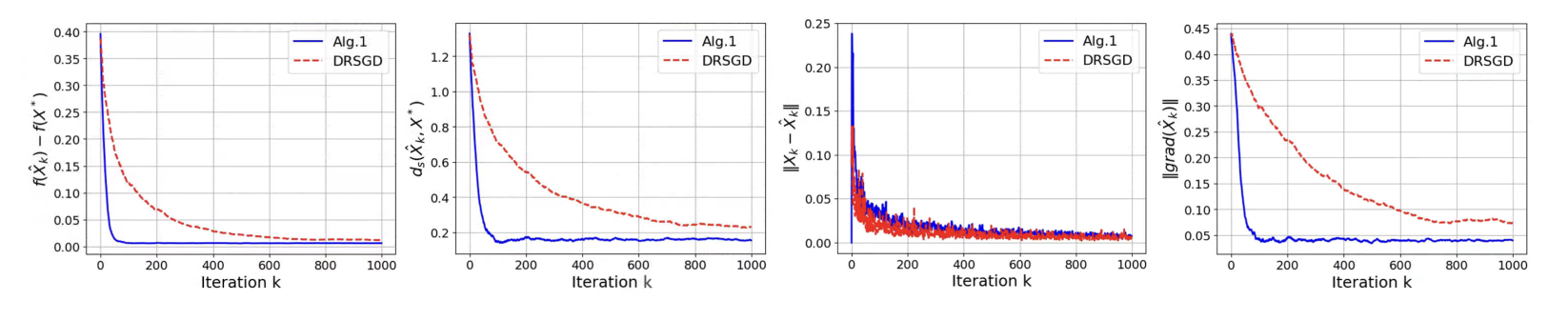
Figure 1: Numerical results on synthetic dataset with DRSGD and Alg.1, eigengap $\triangle=0.8$, Graph:ring, t= 1.

In this section, we conduct some experiments to show the empirical performance of Algorithm 1 on the principal component analysis problems.

Principal component analysis (PCA) dimension reduction is with extensive applications in machine learning. It can be formulated as follows:

$$\min_{X_{i}\in\text{St}(n,r)} \ -\frac{1}{2N}\sum_{i=1}^{N}X_{i}^{\top}A_{i}^{\top}A_{i}X_{i},$$ (58)

$$s.t. \ X_{1}=\dots=X_{N},$$

where $A_{i}\in\mathbb{R}^{m_{i}\times n}$ is the local data matrix of agent $i$ and $m_{i}$ is the data size. Denote by $A:=[A_{1}^{\top},\dots,A_{N}^{\top}]$ the global data matrix. We also utilize the Bluefog [36] package to conduct a distributed structure and Pymanopt [31] toolbox to compute on the Stiefel manifold.

We run $N=4$ CPU nodes and fix $m_{1}=\dots=m_{4}=2500$, $n=8$ and $r=3$. We generate the data matrix $A$ including $2500N\times n$ i.i.d samples following standard multi-variate Gaussian distribution, and $A_{i}$ is obtained by distributing $A$ into the $4$ CPU nodes. As $X^{*}Q$ is also a solution of (58) with an orthogonal matrix $Q\in\mathbb{R}^{r\times r}$, we define by $d_{s}(X,X^{*})=\min_{Q\in\mathbb{R}^{r\times r},Q^{\top}Q=QQ^{\top}=I_{r}}\|XQ-X^{*}\|$ to measure the distance between $X$ and $X^{*}$. The algorithms are measured by four metrics, i.e., the objective function $f(\hat{X}_{k})-f^{*}$, the distance to the global optimum $d_{s}(X_{k},X^{*})$, the consensus error $\|\mathbb{X}_{k}-\mathbb{\hat{X}}_{k}\|$, and the gradient norm $\|\text{grad}f(\hat{X}_{k})\|$, respectively.

We then compare our algorithm with the state-of-art distributed stochastic optimization algorithm DRSGD in [7] and receive the results in Fig.1. Here we let the communication graph among the four agents to be ring graph. Furthermore, we set the variable sample size of Alg.1 to be $N_{k}=k+1$ which increases in a polynomial rate. Let the multi-steps of consensus $t=1$, the step sizes $\alpha=1$, and $\beta=0.1$ for Alg.1 and be diminishing for DRSGD, respectively. We set the maximum iteration rounds to $1000$ and run Alg.1. The results can be seen in Fig.1 which illustrate that Alg.1 converges faster than DRSGD. Although we have equipped a multi-step communication to achieve the theoretic consensus of the algorithm, the empirical results in Fig.1 show that both of the algorithms achieve consensus with only one communication step in practice.

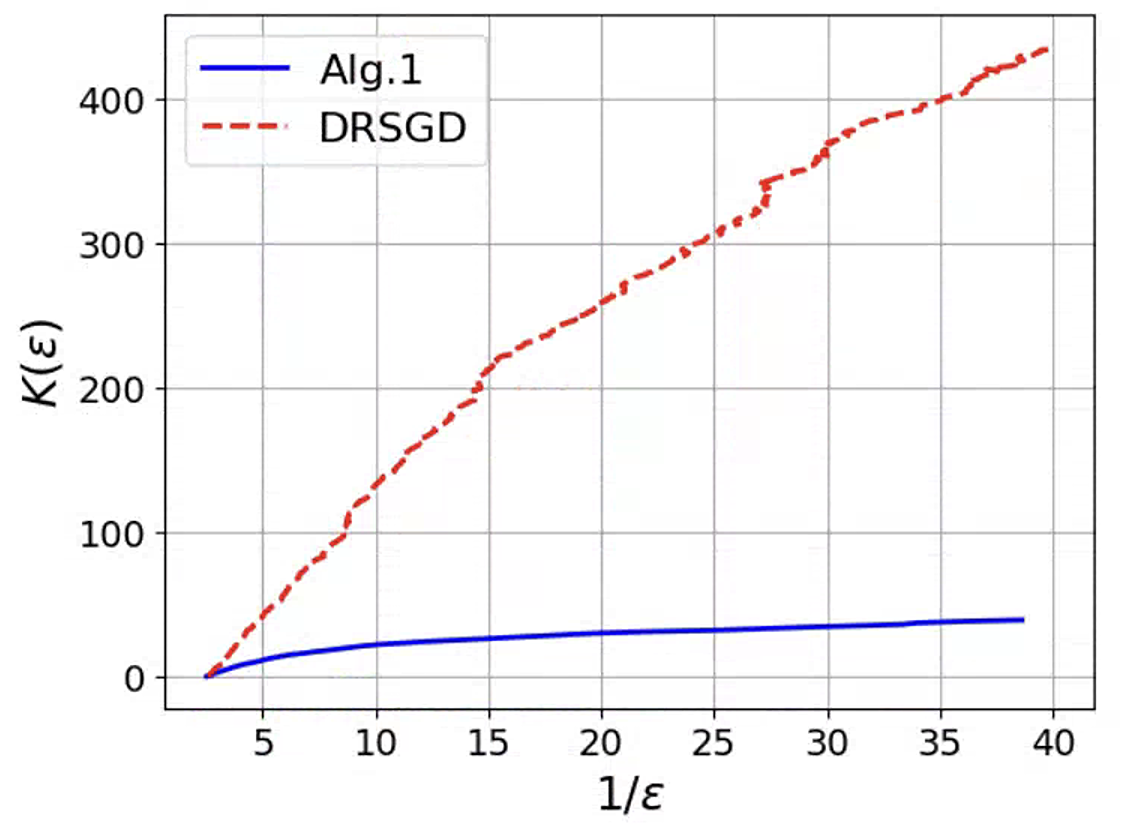
Figure 2: Iteration complexity of Alg.1 and DRSGD

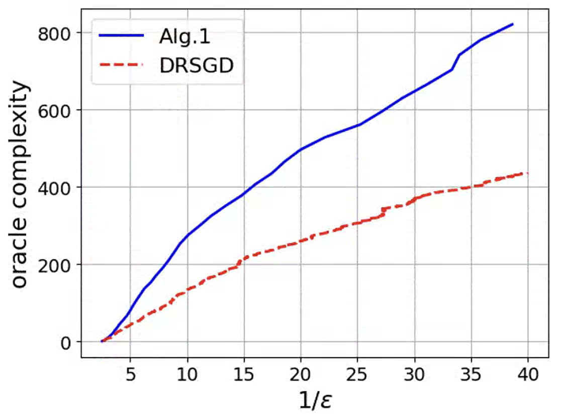
Figure 3: Oracle complexity of Alg.1 and DRSGD

We further compare the iteration and oracle complexity of the two algorithms under the above settings. As shown in Fig.2, to achieve an $\epsilon$-stationary point with the same accuracy, Alg.1 requires much less iteration rounds than DRSGD, which also means it can significantly reduce the communication rounds. However, Fig.3 shows that Alg.1 needs more sampled gradients than DRSGD. The results illustrate that our algorithm can significantly reduce the communication and computation costs by partly sacrificing the amount of gradient samples.

In addition, we conduct experiment to see the impact of the sample sizes. We run Alg.1 with step sizes $\alpha=1,\beta=0.1$ and let $N_{k}=1,k+1,[0.9^{-k}]$ and $N_{k}=[0.85^{-k}],[0.9^{-k}],[0.95^{-k}]$, respectively. The performance of algorithm for both cases are displayed in Fig.4 and Fig.5 which illustrate that a faster increasing sample size leads to a better convergence rate and stability, meanwhile costs more sampled data and heavier computations per one iteration.

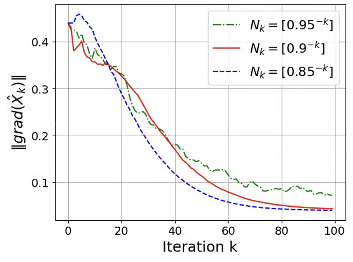
Figure 4: The performance of Alg.1 with $N_{k}=[0.85^{-k}],[0.9^{-k}],[0.95^{-k}]$ under a ring graph.

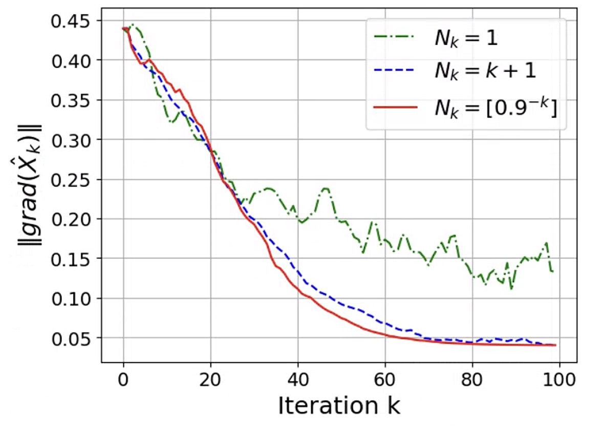
Figure 5: The performance of Alg.1 with $N_{k}=1,k+1,[0.9^{-k}]$ under a ring graph.

6 Conclusion

In this paper, we have proposed a distributed Riemannian stochastic gradient tracking algorithm with variable sample sizes for optimization on the Stiefel manifold over connected networks. If the agents are set to start from a suitably defined local region, we prove that the iterates of all agents always remain in this region and converge to a stationary point (or neighborhood) with fixed step sizes in expectation. We further show that the convergence rate can be affected by the increasing sample size, which can reduce the noise variance. The convergence rate of the iterates with a exponentially increasing sample size is comparable to the non-stochastic framework on the Stiefel manifold. We also give analysis on the convergence rate with polynomially increasing sample size and a constant sample size. Based on the convergence results, we establish the iteration, oracle, and communication complexity, and present the trade-off between communication costs and gradient sampling. Finally, we conduct numerical experiments that demonstrate the effectiveness of the algorithm and the theoretical results. The extension to nonsmooth framework or general compact submanifolds are promising future research directions.

Appendix A Proof of Lemma 9

(i) We begin with analyzing the gradient tracking error of $k+1$. Denote $J=\frac{1}{N}\bm{1}_{N}\bm{1}_{N}^{\top}$. According to Lemma 8, we have

$$\mathbb{Y}_{k+1}-\bar{\mathbb{F}}_{k+1}= (I_{N}\otimes I_{n})\mathbb{Y}_{k+1}-(J\otimes I_{n})\mathbb{Y}_{k+1}$$

$$= ((I_{N}-J)\otimes I_{n})\mathbb{Y}_{k+1}.$$

By plugging (13) in the above inequality, it follows that

$$\mathbb{Y}_{k+1}-\bar{\mathbb{F}}_{k+1}$$

$$= ((I_{N}-J)\otimes I_{n})((W^{t}\otimes I_{n})\mathbb{Y}_{k}+F(\mathbb{X}_{k+1})-F(\mathbb{X}_{k}))$$

$$= ((W^{t}-J)\otimes I_{n})\mathbb{Y}_{k}+((I_{N}-J)\otimes I_{n})(F(\mathbb{X}_{k+1})-F(\mathbb{X}_{k})),$$

where the last equality follows by the doubly stochastic of $W^{t}$ from Assumption 1 (2) and Remark 3. Then by using Lemma 8, we have

$$\mathbb{Y}_{k+1}-\bar{\mathbb{F}}_{k+1}$$

$$= (W^{t}\otimes I_{n})\mathbb{Y}_{k}-\bar{\mathbb{F}}_{k}+((I_{N}-J)\otimes I_{n})(F(\mathbb{X}_{k+1})-F(\mathbb{X}_{k})).$$

Take the norm of the equation above, it follows that

$$\|\mathbb{Y}_{k+1}-\bar{\mathbb{F}}_{k+1}\|_{F}\leq \|(W^{t}\otimes I_{n})\mathbb{Y}_{k}-\bar{\mathbb{F}}_{k}\|_{F}$$ (59)

$$+ \|((I_{N}-J)\otimes I_{n})(F(\mathbb{X}_{k+1})-F(\mathbb{X}_{k}))\|_{F}.$$

Recalling the fact that $\sigma_{2}$ is the spectral norm of $W-J$ stated in Remark 3, we have

$$\|(W^{t}\otimes I_{n})\mathbb{Y}_{k}-\bar{\mathbb{F}}_{k}\|_{F}= \|((W^{t}-J)\otimes I_{n})(\mathbb{Y}_{k}-\bar{\mathbb{F}}_{k})\|_{F}$$ (60)

$$\leq \|W^{t}-J\|_{F}\|(\mathbb{Y}_{k}-\bar{\mathbb{F}}_{k})\|_{F}$$

$$\leq \sigma_{2}^{t}\|\mathbb{Y}_{k}-\bar{\mathbb{F}}_{k}\|_{F}.$$

Substituting (60) to (59) yields

$$\|\mathbb{Y}_{k+1}-\bar{\mathbb{F}}_{k+1}\|_{F}\leq\sigma_{2}^{t}\|\mathbb{Y}_{k}-\bar{\mathbb{F}}_{k}\|_{F}+\|F(\mathbb{X}_{k+1})-F(\mathbb{X}_{k})\|_{F}.$$ (61)

Applying the iteration Lemma 7 to (61), we finally prove (9).

(ii) We begin with presenting the one step improve of consensus. If $\mathbb{X}_{k}\in\mathcal{S}$, using the definition of IAM in (3), we have

$$\|\mathbb{X}_{k+1}-\mathbb{\hat{X}}_{k+1}\|_{F}^{2}\leq\|\mathbb{X}_{k+1}-\mathbb{\hat{X}}_{k}\|_{F}^{2}.$$

Since $X_{i,k}\in\text{St}(n,r)$ and $-\alpha\text{grad}\ h_{i,t}(\mathbb{X}_{k})-\beta v_{i,k}\in T_{X_{i,k}}\mathcal{M}$, by using (19) and the property of retraction in Lemma 1, we get

$$\|\mathbb{X}_{k+1}-\mathbb{\hat{X}}_{k+1}\|_{F}^{2}= \sum_{i=1}^{N}\|\mathcal{R}_{X_{i,k}}(-\alpha\text{grad}\ h_{i,t}(\mathbb{X}_{k})-\beta v_{i,k})-\hat{X}_{k}\|_{F}^{2}$$

$$\leq \sum_{i=1}^{N}\|X_{i,k}-\alpha\text{grad}\ h_{i,t}(\mathbb{X}_{k})-\beta v_{i,k}-\hat{X}_{k}\|_{F}^{2}$$

$$= \|\mathbb{X}_{k}-\mathbb{\hat{X}}_{k}-\alpha\text{grad}\ h_{t}(\mathbb{X}_{k})-\beta\mathbb{v}_{k}\|_{F}^{2}.$$

Since $v_{i,k}=\mathcal{P}_{T_{X_{i,k}}\mathcal{M}}Y_{i,k}$, by the nonexpansiveness of the orthogonal projection, we obtain $\|\mathbb{v}_{k}\|_{F}\leq\|\mathbb{Y}_{k}\|_{F}$, which implies

$$\|\mathbb{X}_{k+1}-\mathbb{\hat{X}}_{k+1}\|_{F}\leq \|\mathbb{X}_{k}-\mathbb{\hat{X}}_{k}-\alpha\text{grad}\ h_{t}(\mathbb{X}_{k})-\beta\mathbb{v}_{k}\|_{F}$$ (62)

$$\leq \|\mathbb{X}_{k}-\mathbb{\hat{X}}_{k}-\alpha\text{grad}\ h_{t}(\mathbb{X}_{k})\|_{F}+\beta\|\mathbb{v}_{k}\|_{F}$$

$$\leq \|\mathbb{X}_{k}-\mathbb{\hat{X}}_{k}-\alpha\text{grad}\ h_{t}(\mathbb{X}_{k})\|_{F}+\beta\|\mathbb{Y}_{k}\|_{F}.$$

Suppose $\mathbb{X}_{k}\in\mathcal{S}$, by Lemma 6, we have

$$\|\mathbb{X}_{k}-\mathbb{\hat{X}}_{k}-\alpha\text{grad}\ h_{t}(\mathbb{X}_{k})\|_{F}^{2}$$

$$= \|\mathbb{X}_{k}-\mathbb{\hat{X}}_{k}\|_{F}^{2}+\|\alpha\text{grad}\ h_{t}(\mathbb{X}_{k})\|_{F}^{2}-2\alpha\langle\mathbb{X}_{k}-\mathbb{\hat{X}}_{k},\text{grad}\ h_{t}(\mathbb{X}_{k})\rangle$$

$$\leq \|\mathbb{X}_{k}-\mathbb{\hat{X}}_{k}\|_{F}^{2}+\left(\alpha^{2}-\frac{\alpha\Phi}{L_{t}}\right)\|\text{grad}\ h_{t}(\mathbb{X}_{k})\|_{F}^{2}.$$

By utilizing (18) in Lemma 5, it follows that

$$\|\mathbb{X}_{k}-\mathbb{\hat{X}}_{k}-\alpha\text{grad}\ h_{t}(\mathbb{X}_{k})\|_{F}^{2}\leq(1-(\alpha L_{t}\Phi-\alpha^{2}L_{t}^{2}))\|\mathbb{X}_{k}-\mathbb{\hat{X}}_{k}\|_{F}^{2}.$$

Let $\rho_{t}^{2}:=1-(\alpha L_{t}\Phi-\alpha^{2}L_{t}^{2})$, and substituting the above result into (62) implies (21). Notice that $\rho_{t}\leq 1$ since $\alpha\leq\frac{\Phi}{L_{t}}$.

By applying Lemma 7 to (21), we finally prove (22).

∎

Appendix B Proof of Lemma 10

We prove this by induction. When $k=0$, by Assumption 4 and Remark 4, and using (11), one has $\|Y_{i,0}\|_{F}=\|F_{i}(X_{i,0})\|\leq A$. Let $\bar{F}_{-1}=\bar{Y}_{0}$. Then for each $i\in\mathcal{N}$,

$$\|Y_{i,0}-\bar{F}_{-1}\|_{F}\leq\|Y_{i,0}\|_{F}+\|\bar{F}_{-1}\|_{F}\leq 2A,$$

while $\mathbb{X}_{0}\in\mathcal{S}$ by the initial selection.

Suppose there exists a $k_{0}$, that for every $0\leq k\leq k_{0}$, we have $\|Y_{i,k}\|_{F}\leq 10A+L_{G}$ and $\|Y_{i,k}-\bar{F}_{k-1}\|_{F}\leq 10A+L_{G}$. It also satisfies that $\mathbb{X}_{k_{0}}\in\mathcal{S}$.

Next, we present the analysis when $k=k_{0}+1$. We first prove that $\mathbb{X}_{k_{0}+1}\in\mathcal{S}$. Based on the induction hypothesis of the bound of $Y_{i,k},k\leq k_{0}$, we can induce the result by a similar argument in the proof of [7, Lem. 4.1]. We include the proof in supplementary for completeness.

Then, by (13) and since $W^{t}$ is doubly stochastic according to Remark 3, we have

$$\|Y_{i,k_{0}+1}-\bar{F}_{k_{0}}\|_{F}$$

$$= \|\sum_{j=1}^{N}W_{ij}^{t}Y_{j,k_{0}}-\bar{F}_{k_{0}}+F_{i}(X_{i,k_{0}+1})-F_{i}(X_{i,k_{0}})\|_{F}$$

$$\leq \|\sum_{j=1}^{N}\left(W_{ij}^{t}-\frac{1}{N}\right)(Y_{j,k_{0}}-\bar{F}_{k_{0}-1})\|_{F}+\|F_{i}(X_{i,k_{0}+1})-F_{i}(X_{i,k_{0}})\|_{F}$$

$$\leq \sigma_{2}^{t}\sqrt{N}\|Y_{j,k_{0}}-\bar{F}_{k_{0}-1}\|_{F}+\|F_{i}(X_{i,k_{0}+1})-F_{i}(X_{i,k_{0}})\|_{F}.$$

By the induction hypothesis that $\|Y_{i,k}-\bar{F}_{k-1}\|_{F}\leq 10A+L_{G}$, it follows that

$$\|Y_{i,k_{0}+1}-\bar{F}_{k_{0}}\|_{F}$$

$$\leq \sigma_{2}^{t}\sqrt{N}(10A+L_{G})+\|\text{grad}f(X_{i,k_{0}+1})-\text{grad}f(X_{i,k_{0}})\|_{F}$$ (63)

$$+ \|F_{i}(X_{i,k_{0}+1})-\text{grad}f_{i}(X_{i,k_{0}+1})\|_{F}+\|F_{i}(X_{i,k_{0}})-\text{grad}f_{i}(X_{i,k_{0}})\|_{F}.$$

By recalling that $\max_{X\in\text{St}(n,r)}\|\text{grad}f_{i}(X)\|_{F}\leq A$ stated in Remark 4, we derive

$$\|F_{i}(X_{i})-\text{grad}f_{i}(X_{i})\|_{F}\leq\|F_{i}(X_{i})\|_{F}+\|\text{grad}f_{i}(X_{i})\|_{F}\leq 2A.$$ (64)

Then by using Lemma 2, and substituting (64) into (B), we further have

$$\|Y_{i,k_{0}+1}-\bar{F}_{k_{0}}\|_{F}\leq\sigma_{2}^{t}\sqrt{N}(10A+L_{G})+L_{G}\|X_{i,k_{0}+1}-X_{i,k_{0}}\|_{F}+4A.$$

Moreover, by using $\sigma_{2}^{t}\leq\frac{1}{2\sqrt{N}}$ since $t\geq[\log_{\sigma_{2}}(\frac{1}{2\sqrt{N}})]$, we get

$$\|Y_{i,k_{0}+1}-\bar{F}_{k_{0}}\|_{F}\leq\frac{1}{2}(10A+L_{G})+4A+L_{G}\|X_{i,k_{0}+1}-X_{i,k_{0}}\|_{F}.$$ (65)

For the last term of the right-hand side, the update of $X_{i,k+1}$ in (19) implies

$$\|X_{i,k_{0}+1}-X_{i,k_{0}}\|_{F}= \|\mathcal{R}_{X_{i,k_{0}}}(-\alpha\text{grad}\ h_{i,t}(\mathbb{X}_{k_{0}})-\beta v_{i,k_{0}})-X_{i,k_{0}}\|_{F}$$ (66)

$$\leq \alpha\|\text{grad}h_{i,t}(\mathbb{X}_{k_{0}})\|_{F}+\beta\|Y_{i,k_{0}}\|_{F}.$$

where the inequality follows by Lemma 1 and $\|v_{i,k_{0}}\|_{F}\leq\|Y_{i,k_{0}}\|_{F}$.

Since $\mathbb{X}_{k_{0}+1}\in\mathcal{S}$, the term $\|\text{grad}h_{i,t}(\mathbb{X}_{k_{0}})\|_{F}$ is bounded by Lemma 5, which implies $\alpha\|\text{grad}h_{i,t}(\mathbb{X}_{k_{0}})\|_{F}\leq 2\delta_{2}\alpha.$ As $\beta\leq\frac{\alpha\delta_{1}}{5(10A+L_{G})}$, and by using the induction hypothesis that $\|Y_{i,k}\|_{F}\leq 10A+L_{G}$, we have $\beta\|Y_{i,k_{0}}\|_{F}\leq\frac{1}{5}\delta_{1}\alpha.$ Substituting these results into (66) implies that

$$\|X_{i,k_{0}+1}-X_{i,k_{0}}\|_{F}\leq 2\delta_{2}\alpha+\frac{1}{5}\delta_{1}\alpha.$$

This together with (65) implies

$$\|Y_{i,k_{0}+1}-\bar{F}_{k_{0}}\|_{F}\leq 9A+\frac{1}{2}L_{G}+2\delta_{2}L_{G}+\frac{L_{G}}{5}\delta_{1}\alpha\leq 9A+L_{G}.$$

According to Assumption 4, we have $\|\bar{F}_{k}\|_{F}\leq A,\forall k\geq 0$, which yields

$$\|Y_{i,k_{0}+1}\|_{F}\leq\|Y_{i,k_{0}+1}-\bar{F}_{k_{0}}\|_{F}+\|\bar{F}_{k_{0}}\|_{F}\leq 10A+L_{G}.$$

Therefore, the proof is completed.

∎

References

- [1] P.-A. Absil, R. Mahony, and Rodolphe Sepulchre. Optimization Algorithms on Matrix Manifolds. Princeton University Press, Princeton, 2008.
- [2] Sulaiman A Alghunaim and Ali H Sayed. Distributed coupled multiagent stochastic optimization. IEEE Transactions on Automatic Control, 65(1):175–190, 2019.
- [3] Silvère Bonnabel. Stochastic gradient descent on Riemannian manifolds. IEEE Transactions on Automatic Control, 58(9):2217–2229, 2013.
- [4] Léon Bottou, Frank E Curtis, and Jorge Nocedal. Optimization methods for large-scale machine learning. SIAM review, 60(2):223–311, 2018.
- [5] Cartis Coralia Boumal Nicolas, Absil P-A. Global rates of convergence for nonconvex optimization on manifolds. IMA Journal of Numerical Analysis, 39(1):1–33, 2018.
- [6] Jun Chen, Haishan Ye, Mengmeng Wang, Tianxin Huang, Guang Dai, Ivor W. Tsang, and Yong Liu. Decentralized Riemannian conjugate gradient method on the Stiefel manifold. arXiv preprint arXiv:2308.10547, 2024.
- [7] Shixiang Chen, Alfredo Garcia, Mingyi Hong, and Shahin Shahrampour. Decentralized Riemannian gradient descent on the Stiefel manifold. In Marina Meila and Tong Zhang, editors, Proceedings of the 38th International Conference on Machine Learning, volume 139 of Proceedings of Machine Learning Research, pages 1594–1605. PMLR, 18–24 Jul 2021.
- [8] Shixiang Chen, Alfredo Garcia, Mingyi Hong, and Shahin Shahrampour. On the local linear rate of consensus on the Stiefel manifold, 2021.
- [9] Kangkang Deng and Jiang Hu. Decentralized projected Riemannian gradient method for smooth optimization on compact submanifolds. arXiv preprint arXiv:2304.08241, 2023.
- [10] Alan Edelman, Tomás A Arias, and Steven T Smith. The geometry of algorithms with orthogonality constraints. SIAM Journal on Matrix Analysis and Applications, 20(2):303–353, 1998.
- [11] Long-Kai Huang and Sinno Pan. Communication-efficient distributed pca by Riemannian optimization. In International Conference on Machine Learning, pages 4465–4474. PMLR, 2020.
- [12] David Kempe and Frank McSherry. A decentralized algorithm for spectral analysis. In Proceedings of the thirty-sixth annual ACM symposium on Theory of computing, pages 561–568, 2004.
- [13] Yann LeCun, Yoshua Bengio, and Geoffrey Hinton. Deep learning. Nature, 521(7553):436–444, 2015.
- [14] Jinlong Lei, Peng Yi, Jie Chen, and Yiguang Hong. Distributed variable sample-size stochastic optimization with fixed step-sizes. IEEE Transactions on Automatic Control, 67(10):5630–5637, 2022.
- [15] Wen Li and Weiwei Sun. Perturbation bounds of unitary and subunitary polar factors. SIAM Journal on Matrix Analysis and Applications, 23(4):1183–1193, 2002.
- [16] Xiao Li, Shixiang Chen, Zengde Deng, Qing Qu, Zhihui Zhu, and Anthony Man-Cho So. Weakly convex optimization over Stiefel manifold using Riemannian subgradient-type methods. SIAM Journal on Optimization, 31(3):1605–1634, 2021.
- [17] Huikang Liu, Anthony Man-Cho So, and Weijie Wu. Quadratic optimization with orthogonality constraint: explicit łojasiewicz exponent and linear convergence of retraction-based line-search and stochastic variance-reduced gradient methods. Mathematical Programming, 178:215–262, 2019.
- [18] Johan Markdahl, Johan Thunberg, and Jorge Goncalves. High-dimensional Kuramoto models on Stiefel manifolds synchronize complex networks almost globally. Automatica, 113:108736, 2020.
- [19] Arkadi Nemirovski, Anatoli Juditsky, Guanghui Lan, and Alexander Shapiro. Robust stochastic approximation approach to stochastic programming. SIAM Journal on Optimization, 19(4):1574–1609, 2009.
- [20] Alex Olshevsky and John N. Tsitsiklis. Convergence speed in distributed consensus and averaging. SIAM Journal on Control and Optimization, 48(1):33–55, 2009.
- [21] S.U. Pillai, T. Suel, and Seunghun Cha. The perron-frobenius theorem: some of its applications. IEEE Signal Processing Magazine, 22(2):62–75, 2005.
- [22] Shi Pu and Angelia Nedić. Distributed stochastic gradient tracking methods. Mathematical Programming, 187:409–457, 2021.
- [23] Guannan Qu and Na Li. Harnessing smoothness to accelerate distributed optimization. IEEE Transactions on Control of Network Systems, 5(3):1245–1260, 2017.
- [24] Haroon Raja and Waheed U Bajwa. Cloud k-svd: A collaborative dictionary learning algorithm for big, distributed data. IEEE Transactions on Signal Processing, 64(1):173–188, 2015.
- [25] Haroon Raja and Waheed U. Bajwa. Cloud k-svd: A collaborative dictionary learning algorithm for big, distributed data. IEEE Transactions on Signal Processing, 64(1):173–188, 2016.
- [26] Herbert Robbins and Sutton Monro. A stochastic approximation method. The Annals of Mathematical Statistics, pages 400–407, 1951.
- [27] Alain Sarlette and Rodolphe Sepulchre. Consensus optimization on manifolds. SIAM Journal on Control and Optimization, 48(1):56–76, 2009.
- [28] Ali H Sayed et al. Adaptation, learning, and optimization over networks. Foundations and Trends® in Machine Learning, 7(4-5):311–801, 2014.
- [29] SUHAIL MOHMAD SHAH. Distributed optimization on Riemannian manifolds. arXiv preprint arXiv:1711.11196, 2017.
- [30] Kunal Srivastava and Angelia Nedic. Distributed asynchronous constrained stochastic optimization. IEEE Journal of Selected Topics in Signal Processing, 5(4):772–790, 2011.
- [31] James Townsend, Niklas Koep, and Sebastian Weichwald. Pymanopt: A python toolbox for optimization on manifolds using automatic differentiation. arXiv preprint arXiv:1603.03236, 2016.
- [32] Eugene Vorontsov, Chiheb Trabelsi, Samuel Kadoury, and Chris Pal. On orthogonality and learning recurrent networks with long term dependencies. In International Conference on Machine Learning, pages 3570–3578. PMLR, 2017.
- [33] Lei Wang and Xin Liu. Decentralized optimization over the Stiefel manifold by an approximate augmented lagrangian function. IEEE Transactions on Signal Processing, 70:3029–3041, 2022.
- [34] Lei Wang and Xin Liu. A variance-reduced stochastic gradient tracking algorithm for decentralized optimization with orthogonality constraints. arXiv preprint arXiv:2208.13643, 2022.
- [35] Jinming Xu, Shanying Zhu, Yeng Chai Soh, and Lihua Xie. Augmented distributed gradient methods for multi-agent optimization under uncoordinated constant stepsizes. In 2015 54th IEEE Conference on Decision and Control (CDC), pages 2055–2060, 2015.
- [36] Bicheng Ying, Kun Yuan, Hanbin Hu, Yiming Chen, and Wotao Yin. Bluefog: Make decentralized algorithms practical for optimization and deep learning. 2021.
- [37] Hongyi Zhang and Suvrit Sra. First-order methods for geodesically convex optimization. In Conference on Learning Theory, pages 1617–1638. PMLR, 2016.