Complementary Search of Fermionic Absorption Operators at Hadron Collider and Direct Detection Experiments

Abstract

Instead of the energy recoil signal at direct detection experiments, dark matter appears always as missing energy at high energy colliders. For a fermionc dark matter coupled with quarks and neutrino via absorption operators, its production is always accompanied by an invisible neutrino. We study in details the mono-X (photon, jet, and $Z$) productions at the Large Hadron Collider (LHC). To make easy comparison between the collider and DM direct detection experiments, we start from the quark-level absorption operators for the first time. In other words, we study the model-independent constraints on a generic fermionic absorption dark fermion. In addition, the interplay and comparison with the possible detection at the neutrino experiment especially Borexino is also briefly discussed. We find that for both spin-dependent and spin-independent absorption of the dark matter, the experiments with light nuclear target can provide the strongest constraints.

1 Introduction

Both astrophysical and cosmological measurements show that dark matter (DM) is an important component of our Universe [1, 2, 3, 4]. However, so far we are still short of direct observations which are necessary clues for the DM model building [5, 9, 8, 10, 7, 6]. The general principle is that the DM should be neutral, massive, and weakly coupled to the Standard Model (SM) particles. In addition, it should be stable enough to have the correct DM relic abundance. Such Weakly Interacting Massive Particle (WIMP) is the most popular DM candidate and its phenomenology has been extensively investigated both theoretically and experimentally.

The DM couplings with the SM particles are mainly constrained by indirect observations [11, 12, 13, 14, 15, 18, 17, 16], direct detections [23, 24, 25, 22, 21, 20, 19], and collider searches [30, 29, 28, 27, 26, 31, 32]. For instance, the DM particles can be indirectly observed by looking for signals of its annihilation into leptons and photons in the high density regions of our Universe [33, 36, 38, 37, 34, 35]. Alternatively, the direct detection experiments investigate the DM interaction with quarks/leptons by searching for the DM collisions with nuclei and electrons inside atom [23, 24, 25, 22, 21, 20, 19], respectively. One of the concrete examples is the absorption of a fermionic DM particle by either nuclei [39, 40, 42, 43, 44, 41, 45, 46] or electron [47, 48, 49, 50, 52, 41, 51] target. The DM particles can also be generated at colliders via the quark/lepton-level interaction operators which are responsible to low energy couplings between the DM and atom [56, 57, 53, 58, 59, 54, 55]. For instance, in the phenomenological model of the DM absorption, the very same interactions can induce single DM production at colliders, and can be probed by investigating missing energy distribution [51, 45].

Usually, the DM particles are produced in pair at colliders as a consequence of some discrete symmetry such as $\mathbb{Z}_{2}$ for guaranteeing the DM stability. However, as long as the DM is light enough, its decay can be slow enough to survive until today as the genuine DM candidate [39, 40, 47, 48, 51]. With high center-of-mass energy, colliders can probe not just the true DM particle that survives until today but also any dark sector particle as long as its direct production is kinematically allowed. This superiority is essentially promising for heavy dark particles that are usually contained in a UV model of the dark sector [64, 61, 60, 62, 63]. Furthermore, the collider search can also provide a tunable environment to distinguish the leptophilic and hadrophilic nature of the DM coupling with SM particles. While hadron colliders mainly probe quark couplings [45, 65, 66, 67, 68], lepton colliders are more sensitive to the leptonic ones [69, 76, 75, 77, 71, 70, 72, 74, 73, 51]. Furthermore, isospin violation and lepton universality of the couplings can also be studied at hadron and lepton colliders, respectively. Therefore, collider search of the DM is not just complementary but also unique for heavy dark particles (or WIMP) [51, 56, 57, 45, 81, 80, 79, 78].

In this paper, we focus on the four-fermion effective operators involving a dark fermion $\chi$ and quarks. While those effective operators with a pair of dark fermion fields [56, 57, 53, 58] can induce elastic scattering off nuclear target in direct detection experiments, they can also be probed at hadron colliders via mono-photon [84, 86, 83, 82, 85], mono-$Z/W$ [84, 94, 91, 93, 89, 87, 88, 92, 90] and mono-jet process [84, 98, 97, 95, 96]. These mono-photon, mono-$Z/W$, and mono-jet channels are also known as mono-$X$ processes [100, 101, 99, 102]. In this paper, we generalize such searches to the four-fermion absorption operators formed by a dark fermion $\chi$, a neutrino, and two quarks. Such interactions can induce the neutral-current dark fermion absorption at the nuclear target [39, 40, 45, 46, 42, 43, 44, 41]. At hadron colliders, the associated production of the dark fermion $\chi$ and the neutrino carries away missing energy to induce the same final-state topology as the dark fermion pair production in the mono-$X$ processes. However, with different kinematic properties of the missing energy, constraints on the relevant parameters can also be significantly different.

The rest of this paper is organized as follows. In Sec. 2, we summarize the four-fermion contact interactions and discuss the interplay of their detecting signals at low- and high-energy experiments. The following Sec. 3 studies the signal and (irreducible) background properties of the mono-$X$ production processes, as well as the constraints from the current LHC data. The details of the mono-photon, mono-jet, and mono-$Z$ productions are given in the subsections Sec. 3.1, Sec. 3.2, and Sec. 3.3, respectively. Then we discuss the projected sensitivities at HL-LHC and HE-LHC in Sec. 3.4. In Sec. 4, we further study the absorption process of a light dark fermion on a nuclei target. Both the spin-independent and spin-dependent scatterings are considered separately in Sec. 4.1 and Sec. 4.2, respectively. Possible interference effects of these two channels for the tensor operator are investigated in Sec. 4.3 and our conclusions can be found in Sec. 5.

2 Fermionic Dark Matter Absorption Operators

In this paper, we study the interactions that can induce the absorption of fermionic DM by nuclei [39, 40, 45, 46, 42, 43, 44, 41]. Instead of transferring the DM kinetic energy into the nuclei recoil energy by elastic scattering, in the absorption process a fermionic DM is converted to a neutrino. Both its mass and kinetic energy are transferred into the nuclei recoil energy. Such processes can be effectively initiated by four-fermion contact interactions [39, 40, 45, 46] which is very similar to the absorption process at electron target [49, 50, 52, 47, 48, 41, 51] .

In the effective field theory (EFT) framework, the interaction operators between the DM and the SM particles are usually constructed according to the SM $SU_{C}(3)\times SU_{L}(2)\times U_{Y}(1)$ gauge symmetries. Assuming that the isospin symmetry is preserved and denoting the first generation up ($u$) and down ($d$) quarks as an isospin doublet $q=(u~{}d)^{T}$, the relevant leading order dim-6 operators connecting the quark and DM-neutrino current can be written as,

$$\mathcal{O}_{S} \equiv(\bar{q}q)\left(\bar{\nu}_{L}\chi_{R}\right)\,,$$ (2.1a)

$$\mathcal{O}_{P} \equiv\left(\bar{q}i\gamma_{5}q\right)\left(\bar{\nu}_{L}\chi_{R}\right)\,,$$ (2.1b)

$$\mathcal{O}_{V} \equiv\left(\bar{q}\gamma_{\mu}q\right)\left(\bar{\nu}_{L}\gamma^{\mu}\chi_{L}\right)\,,$$ (2.1c)

$$\mathcal{O}_{A} \equiv\left(\bar{q}\gamma_{\mu}\gamma_{5}q\right)\left(\bar{\nu}_{L}\gamma^{\mu}\chi_{L}\right)\,,$$ (2.1d)

$$\mathcal{O}_{T} \equiv\left(\bar{q}\sigma_{\mu\nu}q\right)\left(\bar{\nu}_{L}\sigma^{\mu\nu}\chi_{R}\right)\,,$$ (2.1e)

as well as their hermitian conjugates. The quark currents $\bar{q}\varGamma q$ with $\varGamma\equiv 1$, $i\gamma_{5}$, $\gamma_{\mu}$, $\gamma_{\mu}\gamma_{5}$ and $\sigma_{\mu\nu}$ should be understood as $\bar{q}\varGamma q=\bar{u}\varGamma u+\bar{d}\varGamma d$ from the isospin symmetry assumption. The above parameterization includes all the five independent Lorentz structures of the quark bilinear and is complete in the sense of that any other dim-6 operator can be written as a linear combination of the above 5 operators by employing $\gamma$-algebra and Fierz transformations [103, 104, 105]. The neutrino is assumed to be left-handed while the dark matter $\chi$ is a Dirac fermion which has both left- and right-handed components. The effective Lagrangian takes the form as,

$$\mathcal{L}_{\text{eff }}=\sum_{i}\frac{1}{\varLambda_{i}^{2}}\mathcal{O}_{i}+\text{h.c.},$$ (2.2)

with each operator having a cut-off scale $\Lambda_{i}$ of the possible fundamental physics.

The four-fermion contact interactions defined in Eq. (2.1) can lead to the associated production of the DM and neutrino at hadron collider. The above EFT description of collider searches can work well as long as the cut-off scale $\varLambda_{i}$ is higher than the collision energy [53] or the mediator mass is much larger than the collision energy [108, 109, 110]. On the other hand, because of running effect of the EFT operators, the operators defined at the TeV scale can turn into a mixture of them at low energy [106, 107, 111, 112, 113, 56, 57]. However, the mixing effect of the effective operators can be numerically relevant only when coupling between the DM and the top quark is switched on [56]. At hadron colliders, the tree-level direct production of the DM particle is sensitive to only the light quarks. Here we assume that the effective operators defined in Eq. (2.1) is only valid for light quarks and hence the mixing effect can be safely neglected. The interaction between the DM and top quark can be searched for via the associated production of top quark(s) and DM at hadron collider while its influences on the running effect can be investigated consistently. We will study this part elsewhere.

3 Constraints from the LHC

3.1 Mono-Photon Production

The mono-photon radiation is one of the most powerful channel to search for dark particles at colliders [84, 86, 83, 82, 85]. The effective operators defined in Eq. (2.1) can induce mono-$\gamma$ events through the initial-state radiation. There are two subprocesses, $q\bar{q}\to\gamma\chi\bar{\nu}$ and $q\bar{q}\to\gamma\bar{\chi}\nu$ via the $t$-channel exchange of an off-shell quark, that can contribute to the signal, as shown in Fig. 1 (a).

Fig. 1: Feynman diagrams of the mono-$\gamma$ process: (a) for the signal operators and (b) for the irreducible background.

Since we have assumed that isospin is conserved in the effective absorptive interactions defined in Eq. (2.1), the parton-level production rates depend only on the quark charges and masses. At the LHC, the light quark masses can be safely neglected. Hence, the signal cross sections at the parton level are universal for all the light quarks except for the charge dependence. The 2D differential cross sections are,

$$\frac{d\hat{\sigma}_{S(P)}^{q}}{dm_{X}^{2}d\cos\theta_{\gamma}} =\frac{Q^{2}_{q}}{128\pi^{3}\varLambda^{4}_{S(P)}}\frac{(m_{X}^{2}-m_{\chi}^{2})^{2}(\hat{s}^{2}+m_{X}^{4})}{\hat{s}^{2}(\hat{s}-m_{X}^{2})m_{X}^{2}\sin^{2}\theta_{\gamma}}\,,$$ (3.1a)

$$\frac{d\hat{\sigma}_{V(A)}^{q}}{dm_{X}^{2}d\cos\theta_{\gamma}} =\frac{Q^{2}_{q}}{768\pi^{3}\varLambda^{4}_{V(A)}}\frac{(m_{X}^{2}-m_{\chi}^{2})^{2}(2m_{X}^{2}+m_{\chi}^{2})\hat{s}}{(\hat{s}-m_{X}^{2})m_{X}^{6}\sin^{2}\theta_{\gamma}}\left(f_{V(A)}+g_{V(A)}\cos\theta_{\gamma}\right)\,,~{}~{}$$ (3.1b)

$$\frac{d\hat{\sigma}_{T}^{q}}{dm_{X}^{2}d\cos\theta_{\gamma}} =\frac{Q^{2}_{q}}{1536\pi^{3}\varLambda^{4}_{T}}\frac{(m_{X}^{2}-m_{\chi}^{2})^{2}(m_{X}^{2}+2m_{\chi}^{2})\hat{s}^{2}}{(\hat{s}-m_{X}^{2})m_{X}^{8}\sin^{2}\theta_{\gamma}}\left(f_{T}+g_{T}\cos\theta_{\gamma}\right)\,,$$ (3.1c)

where $\hat{s}$ is the center-of-mass energy at the parton level, $\theta_{\gamma}$ is the photon polar angle in the center-of-mass frame, and $m_{X}^{2}\equiv(p_{\nu}+p_{\chi})^{2}$ is the DM-neutrino invariant mass. For convenience, we have defined the following functions $f_{V,A,T}$ and $g_{V,A,T}$,

$$f_{V(A)} \equiv 1+2z_{X}+10z_{X}^{2}+2z_{X}^{3}+z_{X}^{4},$$ (3.2a)

$$g_{V(A)} \equiv(1-z_{X})^{2}(1+4z_{X}+z_{X}^{2}),$$ (3.2b)

$$f_{T} \equiv 17-4z_{X}+7z_{X}^{2}+56z_{X}^{3}+55z_{X}^{4}-4z_{X}^{5}+z_{X}^{6},$$ (3.2c)

$$g_{T} \equiv(1-z_{X})^{3}(15+33z_{X}+15z_{X}^{2}+z_{X}^{3}),$$ (3.2d)

in terms of $z_{X}\equiv m_{X}^{2}/\hat{s}$.

One can see that, there are collinear singularities encoded as the factor $\sin\theta_{\gamma}$ in the denominators of Eq. (3.1) for all the signal operators. There are also soft singularities when the DM-neutrino invariant mass approaches the center-of-mass energy, $m_{X}^{2}\to s$. Such singularities can be cured by cutting the photon transverse momentum and the DM-neutrino invariant mass. The irreducible background also has collinear and soft singularities that come from the associated production of a photon and a $Z$ boson followed by the invisible decay $Z\to\nu\bar{\nu}$.

The channels, $q\bar{q}^{\prime}\to\gamma W^{\pm}(\ell^{\pm}\nu)$ and $q\bar{q}\to\gamma Z(\ell\ell)$ with lepton(s) not detected as well as $q\bar{q}^{\prime}(qg/gg)\to\gamma q\bar{q}^{\prime}(qg/qq)$ with the final-state quark(s)/gluon escaping the detector, can also contribute to the total background. Fortunately, they can be significantly reduced by requiring large transverse missing energy. Hence, here we study kinematical distribution of the background only for the irreducible channel, i.e., $q\bar{q}\to\gamma Z(\nu\nu)$.

The panels (a) and (b) of Fig. 2 show the photon normalized polar angle $\theta_{\gamma}$ and transverse momentum $p_{T,\gamma}$ distributions in the laboratory frame at LHC-13 ($\sqrt{s}=13\,{\rm TeV}$ and a total luminosity $\mathcal{L}=139\,{\rm fb}^{-1}$). The signal properties (colorful non-solid curves) are illustrated with $m_{\chi}=0\,{\rm GeV}$ and $\varLambda_{i}=1\,{\rm TeV}$. As expected, the signal events are dominant at the forward and backward regions which is similar as the irreducible background distribution (black-solid curve). We can also see in Fig. 2 (b) that both the signal and background events mostly distribute in the soft $p_{T,\gamma}$ region. Furthermore, the signal distributions are larger than the background for $p_{T,\gamma}\gtrsim 200\,{\rm GeV}$. Hence $p_{T,\gamma}=200\,{\rm GeV}$ is a good cut to enhance the signal significance. Fig. 2 (c) shows the dependence of the total parton-level cross sections of the signal and the irreducible background on the center-of-mass energy $\sqrt{\hat{s}}$. While the background decreases quickly with increasing $\sqrt{\hat{s}}$, the signals grow rapidly and exceed the background around $\sqrt{\hat{s}}=(700\sim 800)\,{\rm GeV}$ which is less than the energy cutoff $\varLambda_{i}=1\,{\rm TeV}$.

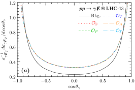
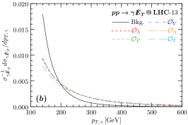
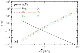
Fig. 2: The normalized parton-level distributions of the photon polar angle ($\theta_{\gamma}$) (a) and transverse momentum ($p_{T,\gamma}$) (b) in the lab frame with the center-of-mass energy $\sqrt{s}=13\,{\rm TeV}$. The panel (c) is the total background and signal cross sections as functions of the center-of-mass energy $\sqrt{\hat{s}}$ at the parton level. In all the above panels, the signals (colorful non-solid curves) are obtained with parameters $m_{\chi}=0\,{\rm GeV}$ and $\varLambda_{i}=1\,{\rm TeV}$ while the background (black-solid curve) stands for the irreducible contribution from the channel $q\bar{q}\to\gamma Z(\nu\nu)$.

The mono-$\gamma$ process has been extensively studied at the LHC for various DM models containing a mediator [114]. It is expected that the same data can give exclusion limits on our model at the same level, i.e., $\varLambda_{i}\sim m_{\rm med}$. Our simulations are conducted using the toolboxes MadGraph [115, 116] and FeynRules [117]. The signal total cross sections are estimated according to the event selections given in the ATLAS search [114]. A photon with a transverse energy above 130 GeV was required at the matrix-element level. A strong kinematical cut ${E\!\!\!/}_{T}\gtrsim 200\,{\rm GeV}$ is used to select the signal events. In this region, the parton shower effect is negligible. So our simulation is done at the generator level. The total detection efficiency is accounted for by an overall normalization factor which is estimated by validating the irreducible background process $pp\to\gamma Z(\nu\nu)$. Consequently, the detector level predictions are obtained by multiplying this normalization factor to the corresponding generator level results.

The left panel of Fig. 3 compares the missing energy distributions between our results and the ATLAS data for the total background (sum of the contributions from the irreducible channel and the other reducible channels). Our prediction on the total background is obtained by rescaling the irreducible background by an overall renormalization factor to match to the total number of the background events. One can see an excellent match in the missing energy distribution and it is clear that within the experimental uncertainty our simulation is valid. The above results indicate that the approximation of an overall normalization factor works well for both the total event number and the differential distributions. This excellent approximation is also employed to estimate the expected exclusion limits on the four-fermion effective operators.

The right panel of Fig. 3 shows the expected exclusion limits at 95% C.L. in the $m_{\chi}-\varLambda$ plane. We can see that the strongest limit is given for the (axial)-vector operator, the constraint on the tensor operator is slightly weaker, and the weakest one is for the (pseudo)-scalar operator. However, the differences are not very significant. In case of $m_{\chi}\sim 0$, the lower bounds are roughly $1.4\,{\rm TeV}$. On the other hand, for $\varLambda_{i}=1\,{\rm TeV}$, a heavy dark fermion with mass from $1.2\,{\rm TeV}$ to $1.5\,{\rm TeV}$ can be excluded.

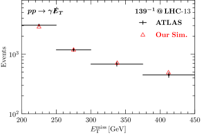
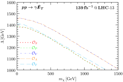
Fig. 3: Light panel: Validation of our simulation for the missing transverse momentum distribution. The experimental data are (black line) taken from the Ref. [114] and our results (red triangle) have been renormalized by multiplying an overall constant. Right panel: The expected 95% C.L. exclusion limits at LHC-13.

3.2 Mono-Jet

The effective operators defined in Eq. (2.1) can also induce mono-jet events. There are three channels which can contribute to the signals and the corresponding Feynman diagrams are shown in Fig. 4 (a), (b) and (c). In contrast to the mono-$\gamma$ process, the mono-jet channel can also be initiated by the gluon components of the incoming hadrons. Hence, stronger constraints on the signal operators are expected. From Fig. 4, one can see that except for the $s$-channel (as shown in the panel (a)), all the other channels are initiated by the initial-state radiation (as shown in the panels (b) and (c)). Hence it is expected that the signals are populated at the forward and backward regions.

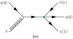
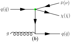
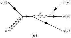
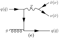
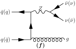
Fig. 4: Feynman diagrams contributing to the mono-jet events. The panels (a), (b) and (c) are for the signal operators while (d), (e) and (f) for the irreducible background.

This is also true for the major background. The associated production of a jet and a $Z$ boson followed by the invisible decays $Z\to\nu\bar{\nu}$ provides the irreducible background whose Feynman diagrams are shown in the Fig. 4 (d), (e) and (f) panels. There are also reducible channels, for instance $q\bar{q}\to W(\tau\nu)$ with the subsequent leptonic decay into $\tau$ that can also contribute to the total background events. In case of $\sqrt{s}=13\,{\rm TeV}$, the total reducible backgrounds contribute about $40\%$ of the total mono-jet events [118]. Here we discuss only physical properties of the irreducible background, i.e., the process $q\bar{q}^{\prime}/qg\to jZ(\nu\bar{\nu})$. In this case, the $Z$ boson comes from either the initial- or final-state radiation. Hence the irreducible backgrounds are also expected to be populated at the forward and backward regions.

The Fig. 5 (a) and (b) show the normalized jet polar angle ($\theta_{j}$) and transverse momentum ($p_{T,j}$) distributions in the laboratory frame, respectively. The signal properties (colorful non-solid curves) are shown for parameters $m_{\chi}=0\,{\rm GeV}$ and $\varLambda_{i}=1\,{\rm TeV}$, and the irreducible background is shown as black-solid curve. Both signals and background are dominant at the forward and backward regions, while the background has a more “collinear singularity” behavior. On the other hand, the signal operators having different Lorentz structure possess completely the same polar angle distribution. So the polar angle cannot distinguish the signal operators. The Fig. 5 (b) panel shows that the signal events are dominant at the soft $p_{T,j}$ region and there are some differences among the five signal operators. Particularly, at the large $p_{T,j}$ region, the distribution for the tensor operator is slightly larger than those for other operators. It turns out that the mono-jet search is more sensitive to the tensor operator. Furthermore, the signal distributions in the region $p_{T,j}\gtrsim 300\,{\rm GeV}$ are larger than the background one. Hence it is a good cut to enhance the signal significance. Fig. 5 (c) shows the variation of the total parton-level cross sections with respect to the center-of-mass energy $\sqrt{\hat{s}}$ for both the signal and the irreducible background. While the background decreases quickly with increasing center-of-mass energy $\sqrt{\hat{s}}$, the signal total cross sections grow rapidly. Similar to the mono-$\gamma$ process, signals exceed the background around $\sqrt{\hat{s}}=900\,{\rm GeV}$.

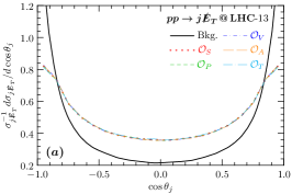
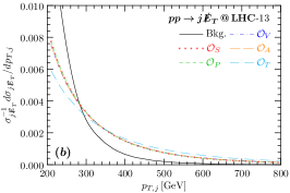
Fig. 5: Normalized parton level distributions of the polar angle ($\theta_{j}$) (a) and transverse momentum ($p_{T,j}$) (b) of the jet in the lab frame with center of mass energy $\sqrt{s}=13\,{\rm TeV}$. (c): total cross sections of the background and signals as functions of the center-of-mass energy at parton level, $\sqrt{\hat{s}}$. In all the three panels, the signal (colorful non-solid curves) are shown for parameters $m_{\chi}=0\,{\rm GeV}$ and $\varLambda_{i}=1\,{\rm TeV}$, and the background (black-solid curve) stands for the irreducible contribution from the channel $q\bar{q}^{\prime}/qg\to jZ(\nu\nu)$.

The ATLAS collaboration searched for new phenomena events containing an energetic jet and a large missing transverse momentum [118]. For an axial-vector mediated model, the exclusion limit for $m_{\chi}=0\,{\rm GeV}$ reaches about $2.1\,{\rm TeV}$. It is expected that the four-fermion contact couplings can be constrained at a similar level. We use those data to constrain the parameters $m_{\chi}$ and $\varLambda_{i}$. In our analysis, events are selected according to the signal region definitions, $E_{T}^{\rm miss}>200\,{\rm GeV}$, $p_{T,j}>150$ GeV and $|\eta_{j}|<2.4$, in [118]. With strong cut on the missing transverse energy, the parton shower effect can be ignored and hence our simulation is done at the generator level. The total detection efficiency is taken into account by an overall normalization factor which is estimated by validating the irreducible background process $pp\to jZ(\nu\nu)$. This overall normalization factor approximation approach is employed to estimate the detector-level prediction for both signal and background.

The left panel of Fig. 6 shows the comparison between our simulation (red square) and the ATLAS result (black dot) for the $p_{T}^{\rm recoil}$ (which is equivelent to the jet transverse missing energy or transverse momentum at the generator level) distribution of the irreducible background channel $pp\to jZ(\nu\bar{\nu})$ at LHC-13 with a total luminosity of $\mathcal{L}=139\,{\rm fb}^{-1}$.

Fig. 6: Left panel: Validation of our simulation for the $p_{T}^{\rm recoil}$ distribution of the irreducible background channel $pp\to jZ(\nu\bar{\nu})$ at the LHC with a total luminosity $\mathcal{L}=139\,{\rm fb}^{-1}$. The experimental data (black dots) are taken from [118] and our results (red rectangles) have been renormalized by multiplying an overall constant. Right panel: The expected 95% C.L. exclusion limits at LHC-13.

The detector effects can be well described in the interested $p_{T}^{\rm recoil}$ region by an overall normalization factor. Within the experimental uncertainty, our simulation is valid. The same normalization factor will be multiplied to the signal cross section to estimate the exclusion limits. It is clear that the approximation of an overall normalization factor works well not only for the total number of events but also the differential distributions. This is particularly important when estimating the exclusion limit with $\chi^{2}$ for the $p_{T}^{\rm recoil}$ distribution.

The right panel of Fig. 6 shows the 95% expected exclusion limits in the $m_{\chi}$-$\varLambda$ plane for our signal operators. We can see that the strongest limit is given for the tensor operator, which can reach to about $3.3\,{\rm TeV}$ for $m_{\chi}\sim 0$. This is because of larger cross section (compared to the other operators), and also more events are populated at the large $p_{T,j}$ region, as shown in Fig. 5 (b). On the other hand, for $\varLambda_{i}=1\,{\rm TeV}$, a heavy dark fermion with mass from $2.6\,{\rm TeV}$ to $3\,{\rm TeV}$ can be excluded. The constraint on the (axial)-vector operator is slightly weaker, $2.6\,{\rm TeV}$ for $m_{\chi}\sim 0$. The weakest one is for the (pseudo)-scalar operator, roughly $2.3\,{\rm TeV}$ for $m_{\chi}\sim 0$. One can also see that, the exclusion limits are about $2$ times stronger than the mono-$\gamma$ one. This is mainly due to the considerably large production cross section of the mono-$j$ process than its mono-$\gamma$ counterpart, as can be seen by comparing Fig. 5 (c) and Fig. 2 (c).

3.3 Mono-$Z$

The effective operators defined in Eq. (2.1) can also induce mono-$Z$ events. There are two channels that can contribute to the signals as shown in Fig. 7 (a) and (b). Similarly, there are also two channels for the major irreducible background $pp\to Z\nu\bar{\nu}$, as depicted in Fig. 7 (c) and (d). In both cases, the $Z$ boson is emitted either by the incoming quark or by the outgoing neutrino. Hence it is expected that both the signal and background are populated in the forward and backward regions.

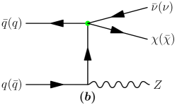
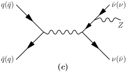
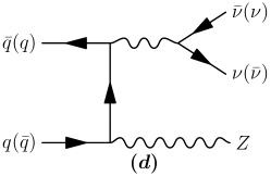
Fig. 7: Feynman diagrams for the mono-$Z$ events, (a) and (b) for the signal while (c) and (d) for the irreducible background.

The Fig. 8 (a) and (b) panels show normalized $Z$ polar angle ($\theta_{Z}$) and transverse momentum ($p_{T,Z}$) distributions in the laboratory frame, respectively. The signals with model parameters $m_{\chi}=0\,{\rm GeV}$ and $\varLambda_{i}=1\,{\rm TeV}$ are shown as colorful non-solid curves while the irreducible background contribution $pp\to Z\nu\bar{\nu}$ as black-solid curve. As expected, both signals and the irreducible background are dominant at the forward and backward regions. For comparison, the background has a more collinear behavior. The reason is twofold. Firstly, the dominant contribution to the irreducible background comes from the $t$-channel di-boson production $q\bar{q}\to ZZ(\nu\nu)$, as shown in Fig. 7 (d). Secondly, compared to the signals, the $s$-channel contribution of the background has a stronger suppression in the large $\hat{s}$ region. One can also see that there are some differences in polar angle distribution among the signal operators having different Lorentz structures, particularly in the forward and backward regions. However, this difference can be dismissed in distinguishing the type of the signal operators because the large background in this region. Furthermore, as one can see from Fig. 8 (b) that the signal events are dominant at the large transverse momentum region and the signals exceed the background in the region $p_{T,Z}\gtrsim 200\,{\rm GeV}$. So the dominant contribution to the signal significance comes from the events having relatively large transverse momentum. The Fig. 8 (c) shows the dependence of the total parton-level cross sections on the center-of-mass energy $\sqrt{\hat{s}}$ for both the signals and the irreducible background. One can clearly see that while the background decreases quickly with the increasing center-of-mass energy $\sqrt{\hat{s}}$, the signal total cross sections grow rapidly with $\sqrt{\hat{s}}$. Again, signals exceed the background around $\sqrt{\hat{s}}=1\,{\rm TeV}$.

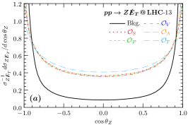
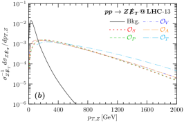
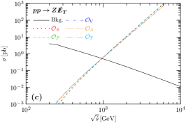
Fig. 8: The normalized parton-level distributions of the polar angle ($\theta_{Z}$, panel (a)) and transverse momentum ($p_{T,Z}$, panel (b)) of the $Z$ boson in the laboratory frame with center-of-mass energy $\sqrt{s}=13\,{\rm TeV}$. Panel (c): the parton-level total cross sections of the background and signals as functions of the center-of-mass energy $\sqrt{\hat{s}}$. The signal (colorful non-solid curves) are shown for parameters $m_{\chi}=0\,{\rm GeV}$ and $\varLambda_{i}=1\,{\rm TeV}$, and the background (black-solid curve) stands for the irreducible contribution from the channel $q\bar{q}\to Z\nu\nu$.

However, it is not straightforward to study the experimental constraints on the model parameters, because the $Z$ reconstruction is necessary in practical measurement. For its leptonic decay modes, since tracks can be measured precisely, mono-$Z$ events can be efficiently selected by putting a cut on the lepton pair invariant mass. However, it is not true for the hadronic decay modes. On one hand, the jet momentum uncertainty is much larger than the lepton counterpart. On the other hand, both the electroweak (for instance $pp\to W^{\pm}(jj)+{E\!\!\!/}_{T}$) and the pure QCD channels $pp\to jj+{E\!\!\!/}_{T}$ can contribute the total background. Factually, the pure QCD contribution completely dominates the total background [119]. So we study the leptonic and hadronic decay modes separately in Sec. 3.3.1 and Sec. 3.3.2.

3.3.1 Leptonic decay modes

Let us study first the mono-$Z$ production followed by leptonic decays $Z\to\ell\ell$ ($\ell=e$ and $\mu$) at the center-of-mass energy $\sqrt{s}=13\,{\rm TeV}$. The left and right panels of Fig. 9 show the normalized polar angle and transverse momentum distributions of the reconstructed $Z$-boson from the two leptons. One can clearly see that for both the signal (colorful non-solid curves) and the irreducible background (black-solid curve), the distinctive kinematic properties (that has been discussed for on-shell production of a $Z$ boson) of the mono-$Z$ events can be readily reconstructed.

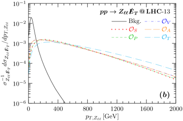
Fig. 9: The normalized distributions of the polar angle ($\theta_{Z_{\ell}}$, left panel) and the transverse momentum ($p_{T,Z}$, right panel) of the reconstructed $Z$ boson from its leptonic decay modes. In both panels, the observables are calculated in the lab frame with the center-of-mass energy $\sqrt{s}=13\,{\rm TeV}$. The signals (colorful non-solid curves) are shown for parameters $m_{\chi}=0\,{\rm GeV}$ and $\varLambda_{i}=1\,{\rm TeV}$ while the background (black-solid curve) stands for the irreducible contribution from $q\bar{q}\to Z\nu\nu$.

The ATLAS collaboration has searched for dark matter in the mono-$Z$ production with the $Z$ boson decaying to two leptons [120]. The major backgrounds come from the irreducible contribution of the resonant $pp\to ZZ\to\ell\ell\nu\nu$ and non-resonant ($pp\to WW\to\ell\ell\nu\nu$, etc. ) channels. In addition, the reducible backgrounds come from the channels $pp\to WZ$ and $pp\to Z+{\rm jets}$. The events are selected by requiring that the leptons must have $p_{T}>20,30$ GeV when ordered with increasing $p_{T}$ and their distance has to fulfill $\Delta R_{\ell\ell}<1.8$. Furthermore, only those events with $E_{T}^{miss}>90\,{\rm GeV}$ and containing exactly two oppositely charged electrons or muons with an invariant mass $76\,{\rm GeV}<m_{\ell\ell}<106\,{\rm GeV}$ around the $Z$ boson mass are selected for further analysis. The signal region is defined by a selection condition $m_{T}\geq 200\,{\rm GeV}$ on the transverse mass $m_{T}$ which is defined as follows,

$$m_{T}=\sqrt{\left[\sqrt{m_{Z}^{2}+(p_{T}^{\ell\ell})^{2}}+\sqrt{m_{Z}^{2}+(E_{T}^{\rm miss})^{2}}\right]^{2}-\left[\vec{p}_{T}^{\;\ell\ell}+\vec{E}_{T}^{\rm miss}\right]^{2}}\,,$$ (3.3)

The transverse mass $m_{T}$ is introduced to select signals from the backgrounds. At the parton level, $\vec{p}_{T}^{\;\ell\ell}=-\vec{E}_{T}^{\rm miss}$, hence the transverse mass is simply given as $m_{T}=\sqrt{2[m_{Z}^{2}+(p_{T}^{\ell\ell})^{2}]}$. As a result, the requirement $m_{T}\geq 200\,{\rm GeV}$ is equivalent to $p_{T}^{\ell\ell}\gtrsim 85\,{\rm GeV}$ which is a relatively strong cut for the parton shower effect. Hence our simulation is done at the generator level.

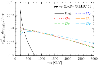
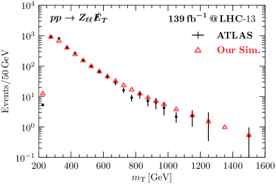
Fig. 10: Left panel: The normalized transverse mass $m_{T}$ distribution using the $Z$ leptonic decay modes ($Z\to\ell\ell$ with $\ell=e,\mu$). The signal distributions (colorful non-solid curves) are illustrated with $m_{\chi}=0\,{\rm GeV}$ and $\varLambda_{i}=1\,{\rm TeV}$ while the background (black-solid curve) stands for the irreducible contribution from $pp\to Z(\ell\ell)\nu\bar{\nu}$. Right panel: The $m_{T}$ distribution of the irreducible background at LHC-13. The experimental data are (black dot) taken from the Ref. [120] and our results (red trangle) have been renormalized by multiplying an overall constant.

The left panel of Fig. 10 shows the normalized transverse mass $m_{\rm T}$ distributions for the signals (colorful non-solid curves) with $m_{\chi}=0\,{\rm GeV}$ and $\varLambda_{i}=1\,{\rm TeV}$ as well as the irreducible background (black-solid curve) from $pp\to Z(\ell\ell)\nu\nu$. One can clearly see that the irreducible background drops very quickly with increasing $m_{T}$ but there are sizable long tails for signals. Hence $m_{T}$ is really a good observable for selecting the signal events. The total detector efficiency is approximated by an overall normalization factor that is estimated by validating the irreducible background $pp\to Z(\ell\ell)\nu\nu$. The right panel of the Fig. 10 compares our simulation (red trangle) with the ATLAS data (black dot) for the $m_{T}$ distribution of the irreducible background $pp\to Z(\ell\ell)\nu\nu$ at LHC-13. One can see that the detector effects can be well modeled (for both the total event number and the differential distibution) by an overall normalization factor. Again we assume that total detector efficiency is universal for both the signals and background. Namely, both the total event number and the $m_{T}$ distribution of the signal events at the detector level are obtained by multiplying the corresponding values at the generator level with the same normalization factor.

Fig. 11 shows the 95% C.L. expected exclusion limits in the $m_{\chi}$-$\varLambda$ plane. The strongest limit is given for the tensor operator and it can reach to about $4.9\,{\rm TeV}$ for $m_{\chi}\sim 0$. This is because of the relatively larger cross section than the other operators (as shown in Fig. 8 (c)) and also more events are populated at the large $m_{T}$ region (as shown in the left panel of the Fig. 10). The constraint on the (pseudo)-scalar operator is slightly weaker which is about $4.5\,{\rm TeV}$ for $m_{\chi}\sim 0$. The weakest one is for the (axial)-vector operator, being roughly $4.2\,{\rm TeV}$ for $m_{\chi}\sim 0$. On the other hand, for $\varLambda_{i}=1\,{\rm TeV}$, a heavy dark fermion with mass up to $4\,{\rm TeV}$ can be excluded.

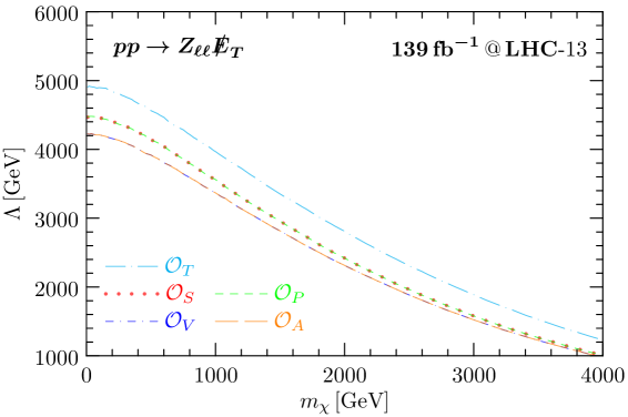
Fig. 11: The expected exclusion limits at 95% C.L. using the mono-$Z$ events at LHC-13. The $Z$-boson is reconstructed by its leptonic decay modes $Z\to\ell\ell$ with $\ell=e,\mu$.

One can also see that the exclusion limits are stronger than the mono-$j$ (and the mono-$\gamma$) process, even through mono-$j$ process has considerably larger cross section which can be seen by comparing Fig. 8 (c) with Fig. 5 (c) and Fig. 2 (c). This is mainly due to the significantly larger background and uncertainty of the mono-$j$ event. Comparing with the mono-$\gamma$ process, the total cross sections are at the same level but the $Z$ transverse momentum distribution (and hence missing transverse momentum and transverse mass) is sizably harder than the photon one. Therefore, we have larger signal significance in the mono-$Z_{\ell\ell}$ event and hence stronger exclusion limits.

3.3.2 Hadronic decay modes

The mono-$Z$ event reconstruction for the hadronic decay mode is much more complex than the leptonic one.

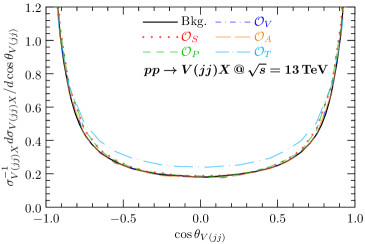
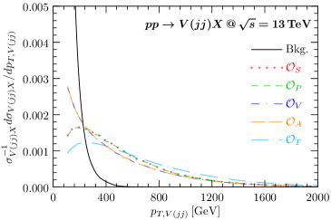
Fig. 12: The normalized polar angle (left panel) and transverse momentum (right panel) distributions of the reconstructed vector boson from two jets with invariant mass $m_{jj}\in[65,\,105]\,{\rm GeV}$ for two channels $pp\to V(jj)+{E\!\!\!/}_{T}$ ($V=Z$ and $W$) at center-of-mass energy $\sqrt{s}=13\,{\rm TeV}$. For both panels, the signal events with parameters $m_{\chi}=0\,{\rm GeV}$ and $\varLambda_{i}=1\,{\rm TeV}$ are illustrated by colorful non-solid curves and the background is shown as black-solid curve.

Firstly, because of the relatively small mass difference between the $W$ and $Z$ bosons as well as the large jet momentum uncertainty, the reconstructed $Z$ bosons are inevitably contaminated by the hadronic $W$ decay products. The left and right panels of Fig. 12 show the normalized polar angle and transverse momentum distributions of the reconstructed vector boson from $pp\to V(jj)+{E\!\!\!/}_{T}$ for both $V=Z$ and $W$. Comparing to the purely mono-$Z$ contribution in Fig. 8 (a), the background is less towards the forward and backward regions. This is due to the large jet transverse energy cut, as shown in Fig. 12 (b).

Secondly, the mono-$Z$ events are even more heavily contaminated by the associated production of missing energy with pure QCD jets. The dominant contribution comes from the associated production of 2-jets with an invisibly decaying $Z$ boson, i.e., the channels $pp\to Z(\nu\nu)+jj$. In this case, the 2 jets with invariant mass in the window $m_{\rm jets}\in[65,\,105]\,{\rm GeV}$ can be miss-identified as a hadronically decaying $Z$ boson. Factually, it consists majority of the total background [119]. Fig. 13 shows the polar angle and transverse momentum distributions of the summed jet ($jj$) for both the signal processes $pp\to\chi\nu+2j$ and the dominant background $pp\to Z(\nu\nu)+2j$. Comparing with Fig. 12, both signal and background are pushed towards the forward and backward regions. Consequently, the transverse momentum of the fake $Z$-boson from QCD jets are softer.

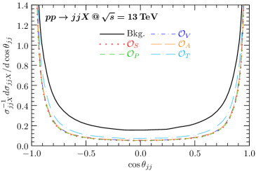
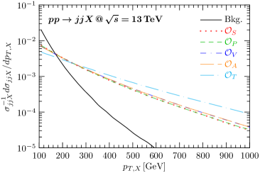
Fig. 13: The normalized polar angle (left) and transverse momentum (right) distributions in the invariant mass window $m_{\rm jets}\in[65,\,105]\,{\rm GeV}$ for the channels $pp\to{E\!\!\!/}_{T}+{\rm jets}$ with QCD jets, respectively. For all the panels, the signal events (colorful non-solid curves) are illustrated with parameters $m_{\chi}=0\,{\rm GeV}$ and $\varLambda_{i}=1\,{\rm TeV}$.

The ATLAS collaboration has searched for dark matter in the mono-$Z/W$ production with hadronically decaying $Z/W$-boson [119] in three categorizations: the high purity (HP) and low purity (LP) regions for merged topology (MT), and the resolved topology (RT). In each region, 3 configurations are defined according to $b$-tagging. Since the background in the RT region is about 1 order larger, our following calculations consider only the LP and HP regions. Furthermore, the contributions with non-zero $b$-tagging number are sub-leading and hence can be ignored.

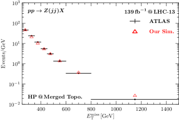
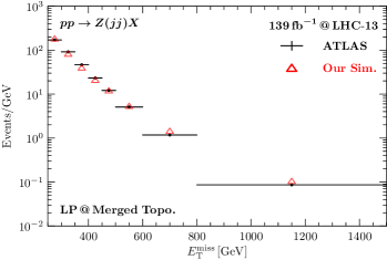
Fig. 14: Validation of our simulation for the missing transverse energy distribution of the pure QCD di-jet production channel $pp\to Z(\nu\nu)+jj$ at the LHC-13 with a total luminosity $\mathcal{L}=36.1\,{\rm fb}^{-1}$. The left and right panels are for the HP and LP regions, respectively. The experimental data [119](black-solid line) and our results (red triangle) have been normalized by multiplying an overall constant.

Fig. 14 compares our simulation (red triangle) and the ATLAS result (black-solid line) for the missing transverse energy distribution of the pure QCD di-jet production channel $pp\to Z(\nu\nu)+jj$ at the LHC-13 with a total luminosity $\mathcal{L}=36.1\,{\rm fb}^{-1}$. The total event number of our result has been normalized to the experimental data. One can see that the detector effects can be properly described by an overall normalization factor. The same normalization factor is then multiplied to the signal cross sections in order to calculate the corresponding exclusion limits.

Fig. 15 shows the 95% expected exclusion limits in the $m_{\chi}$-$\varLambda$ plane for our signal operators. The strongest limit comes from the tensor operator. With $m_{\chi}\sim 0$, the lower limits can reach $2.6$ and $2.9\,\,{\rm TeV}$ in the HP and LP regions, respectively. The constraint on the (pseudo)-scalar operator that can reach $2.3$ and $2.6\,{\rm TeV}$ in the HP and LP regions, respectively, with $m_{\chi}\sim 0$ is slightly weaker. The weakest constraint happens for the (axial)-vector operator which is only about $1.8$ and $2.0\,{\rm TeV}$ in the HP and LP regions, respectively. On the other hand, for a given energy scale $\varLambda_{i}=1\,{\rm TeV}$, a heavy dark fermion with mass from $2\,{\rm TeV}$ to $4\,{\rm TeV}$ can be excluded.

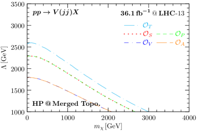
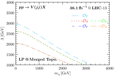
Fig. 15: The expected exclusion limits at 95% C.L. using the mono-$Z/W$ events with hadronically decaying $Z/W$ boson at LHC-13. The left and right panels are for the HP and LP regions, respectively.

3.4 Future Sensitivities

This section studies the future sensitivities at the upgraded versions of LHC [121]. As discussed in the last sections, the signal cross sections grow with the center-of-mass energy while the background one decreases. It is then expected that the future upgrades of LHC have great advantages for probing the four-fermion coupling operators. Furthermore, the upgrades will accumulate much larger luminosity. Table 1 lists the studied configurations and the the parton-level kinematic cuts.

Process	14 TeV, 3$\,{\rm ab}^{-1}$(LHC-14)	25 TeV, 20$\,{\rm ab}^{-1}$(LHC-25)
$pp\to\gamma{E\!\!\!/}_{T}$	$p_{T,\gamma}\geqslant 200\,\,{\rm GeV}$ ,  $\big{|}\eta_{\gamma}\big{|}\leqslant 2.5$ ${E\!\!\!/}_{T}\geqslant 200\,\,{\rm GeV}$	$p_{T,\gamma}\geqslant 400\,\,{\rm GeV}$ ,  $\big{|}\eta_{\gamma}\big{|}\leqslant 2.5$ ${E\!\!\!/}_{T}\geqslant 400\,\,{\rm GeV}$
$pp\to j{E\!\!\!/}_{T}$	$p_{T,j}\geqslant 200\,\,{\rm GeV}$ ,  $\big{|}\eta_{j}\big{|}\leqslant 2.4$ ${E\!\!\!/}_{T}\geqslant 200\,\,{\rm GeV}$	$p_{T,j}\geqslant 400\,\,{\rm GeV}$ ,  $\big{|}\eta_{j}\big{|}\leqslant 2.4$ ${E\!\!\!/}_{T}\geqslant 400\,\,{\rm GeV}$
$pp\to Z(\ell^{+}\ell^{-}){E\!\!\!/}_{T}$	${E\!\!\!/}_{T}\geqslant\,85\,\,{\rm GeV}$ $p_{T,\ell}\geqslant 50\,\,{\rm GeV}$ ,  $\big{|}\eta_{\ell}\big{|}\leqslant 2.47$	${E\!\!\!/}_{T}\geqslant 178\,\,{\rm GeV}$ $p_{T,\ell}\geqslant 100\,\,{\rm GeV}$  ,  $\big{|}\eta_{\ell}\big{|}\leqslant 2.47$
$pp\to V(q\bar{q}){E\!\!\!/}_{T}$	${E\!\!\!/}_{T}\geqslant\,200\,\,{\rm GeV}$ $p_{T,j}=20\,\,{\rm GeV}$ ,  $\big{|}\eta_{j}\big{|}\leqslant 4.5$ $m_{jj}\in\big{[}65,\,105\big{]}\,\,{\rm GeV}$	${E\!\!\!/}_{T}\geqslant\,400\,\,{\rm GeV}$ $p_{T,j}=40\,\,{\rm GeV}$  ,  $\big{|}\eta_{j}\big{|}\leqslant 4.5$ $m_{jj}\in\big{[}65,\,105\big{]}\,\,{\rm GeV}$

Table 1: The upgraded configurations of LHC and the corresponding parton-level kinematic cuts [121].

Fig. 16 and Fig. 17 show the expected 95% C.L. exclusion limits using the mono-$\gamma$, mono-$j$, mono-$Z_{\ell\ell}$, and mono-$V_{jj}$ (combined results of the HP and LP regions) events at the LHC-14 (left) and LHC-25 (right), respectively.

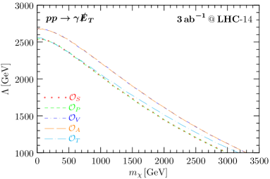
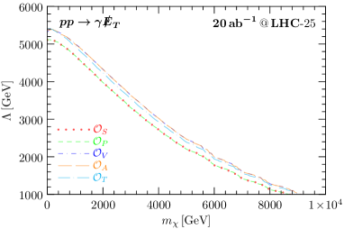
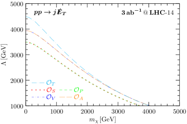
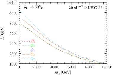
Fig. 16: The expected 95% C.L. exclusion limits from the mono-$\gamma$ (upper) and mono-$j$ events (lower) at LHC-14 (left) and LHC-25 (right).

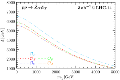
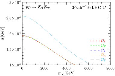
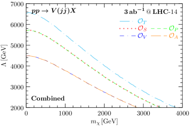
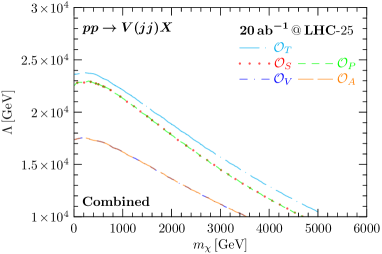
Fig. 17: The expected 95% C.L. exclusion limits from the mono-$Z_{\ell\ell}$ (upper) and mono-$V_{jj}$ events (lower) at LHC-14 (left) and LHC-25 (right).

One can clearly see the constraint improvements, although the enhancements vary from process to process. However, for all the processes, there is roughly a factor of 1.5 and 3 enhancement on the lower bounds of the energy scale $\Lambda_{i}$ (for $m_{\chi}=0$) at the LHC-14 and LHC-25 configurations, respectively.

4 Absorptions at Nuclear Target

The parton-level operators defined in Eq. (2.1) inevitably lead to signals at the hadron level that can be investigated by the DM direct detection experiments. The DM is converted to an active neutrino and its mass fully absorbed to generate large nucleus recoil energy [39, 40],

$$\chi(p_{\chi})+A(p_{i})\rightarrow\nu(p_{\nu})+A(p_{f})\,,$$ (4.1)

where we have used the mass number $A$ to denote the nucleus target. Those momenta of the initial and final states are explicitly specified in parenthesis. The differential scattering rate per nuclear recoil energy $E_{R}$ is given as,

$$\frac{{\rm d}R_{A}}{{\rm d}E_{R}}=N_{A}n_{\chi}\int\mathrm{d}^{3}\bm{v}_{\chi}f_{\mathrm{E}}(\boldsymbol{v}_{\chi},t)v_{\chi}\frac{\mathrm{d}\sigma_{A}}{\mathrm{~{}d}E_{\mathrm{R}}}\,,$$ (4.2)

where $N_{A}$ is the number of nuclear targets. If there are more than one isotope, the total rate is simply the sum of the individual contributions. In addition, $n_{\chi}=\rho_{\chi}/m_{\chi}$ is the local number density of the DM with the local dark matter energy density $\rho_{\chi}\simeq 0.3{\,\rm GeV/cm}^{3}$. The differential cross section ${\rm d}\sigma_{\rm A}/{\rm d}E_{\rm R}$ defined in Eq. (4.1) is averaged over the incoming DM velocity distribution $f_{\mathrm{E}}(\boldsymbol{v}_{\chi},t)$.

In contrast to the usual elastic and inelastic scatterings, the absorption process has quite different kinematics. For a non-relativistic DM, the nucleus recoil energy, $E^{0}_{R}=m_{\chi}^{2}/2(m_{A}+m_{\chi})$, is roughly proportional to the DM mass squared $m^{2}_{\chi}$ at the leading order with $m_{\chi}$ much smaller than the nucleus mass $m_{A}$. So the differential cross section ${\rm d}\sigma_{\rm A}/{\rm d}E_{R}$ exhibits a sharp peak at $E^{0}_{R}$,

$$\frac{{\rm d}\sigma_{A}}{{\rm d}E_{\rm R}}=\frac{\overline{\big{|}\mathcal{M}_{A}\big{|}^{2}}}{16\pi m_{A}^{2}v_{\chi}}\delta\big{(}E_{R}-E_{R}^{0}\big{)}\,,$$ (4.3)

where $\overline{|M_{A}|^{2}}$ is the squared amplitude of the process in Eq. (4.1) with helicity average and summation over the initial and final states, respectively. For a nucleus with total spin $J$, the explicit definition of $\overline{|M_{A}|^{2}}$ is given as,

$$\overline{|\mathcal{M}_{A}|^{2}}\equiv\frac{1}{2s_{\chi}+1}\frac{1}{2J+1}\sum_{\begin{subarray}{c}\text{ initial \& }\\ \text{ final spins }\end{subarray}}|\mathcal{M}_{A}|^{2}\,,$$ (4.4)

where $s_{\chi}=1/2$ is the DM spin. With a non-relativistic DM, i.e., $m_{\chi}\gg p_{\chi}$, the dominant contribution to the amplitude is given by the limit $p_{\chi}\to 0$. Therefore, at leading order, amplitude of the absorption process, $\mathcal{M}_{A}$ is independent of the DM velocity. In this case, the velocity integral in Eq. (4.2) can be carried out independently. Inserting Eq. (4.3) into Eq. (4.2), the DM velocity dependence can be completely removed since the DM velocity distribution function should be normalized to 1. In practice, there is also a threshold of the recoil energy, $E_{\rm R}^{\rm th}$, which is the minimal energy that can be detectable in a specific experiment,

$$\frac{\mathrm{d}R_{A}}{\mathrm{d}E_{\mathrm{R}}}=\frac{N_{A}n_{\chi}}{16\pi m_{A}^{2}}\overline{\big{|}\mathcal{M}_{A}\big{|}^{2}}\delta\big{(}E_{R}-E_{R}^{0}\big{)}\varTheta(E_{\rm R}-E_{\rm R}^{\rm th})\,.$$ (4.5)

Although both coherent and incoherent scatterings can contribute to the direct detection of absorption DM [46], we consider only the coherent one for simplicity and easy comparison with experimental analysis. Both the spin-independent (SI) and spin-dependent (SD) interactions can happen depending on the Lorentz structure of the various effective operators under study. The nucleus-level amplitude $\mathcal{M}_{A}$ can be written as,

$$\mathcal{M}_{A}(q^{2})=\sum_{N=p,n}F_{\rm Res}^{N}(q^{2})\mathcal{M}_{\rm PLN}^{N}(q^{2})=\sum_{N=p,n}F_{\rm Res}^{N}(q^{2})C_{N}\mathcal{M}_{N}(q^{2})\,,$$ (4.6)

where $q^{2}\equiv(p_{f}-p_{i})^{2}=(p_{\nu}-p_{\chi})^{2}$ is the squared momentum transfer and $F_{\rm Res}^{N}(q^{2})$ are the corresponding response functions. The amplitude for the DM scattering off a point-like nucleus (PLN) $\mathcal{M}_{\rm PLN}^{N}(q^{2})$ is related to the scattering amplitude $\mathcal{M}_{N}(q^{2})$ off a single nucleon (with nucleon mass normalized to $m_{A}$). The difference between the SI and SD interactions are distinguished by a coherence factor $C_{N}$. For the SI scattering, $C_{N}=Z$ and $A-Z$ for proton and neutron, respectively, while $C_{N}=1$ for its SD counterpart.

In order to caculate the DM direct detection event rate according to Eq. (4.5), the quark-level operators in Eq. (2.1) should be converted to the nucleon-level matrix elements [56, 130, 128, 129],

$$\langle N|m_{q}\bar{q}q|N\rangle =F_{S}^{q/N}(q^{2})\overline{u}_{N}u_{N}\,,$$ (4.7a)

$$\langle N|m_{q}\bar{q}i\gamma_{5}q|N\rangle =F_{P}^{q/N}(q^{2})\overline{u}_{N}i\gamma_{5}u_{N}\,,$$ (4.7b)

$$\langle N|\bar{q}\gamma^{\mu}q|N\rangle =\overline{u}_{N}\bigg{[}F_{1}^{q/N}(q^{2})\gamma^{\mu}+\frac{i\sigma^{\mu\nu}q_{\nu}}{2m_{N}}F_{2}^{q/N}(q^{2})\bigg{]}u_{N}\,,$$ (4.7c)

$$\langle N|\bar{q}\gamma^{\mu}\gamma_{5}q|N\rangle =\overline{u}_{N}\bigg{[}F_{A}^{q/N}(q^{2})\gamma^{\mu}\gamma_{5}+\frac{\gamma_{5}q^{\mu}}{2m_{N}}F_{P^{\prime}}^{q/N}(q^{2})\bigg{]}u_{N}\,,$$ (4.7d)

$$\langle N|m_{q}\bar{q}\sigma^{\mu\nu}q|N\rangle =\overline{u}_{N}\bigg{[}F_{T,0}^{q/N}(q^{2})\sigma^{\mu\nu}+\frac{i\gamma^{[\mu}q^{\nu]}}{2m_{N}}F_{T,1}^{q/N}(q^{2})+\frac{iq^{[\mu}p^{\nu]}}{m_{N}^{2}}F_{T,2}^{q/N}(q^{2})\bigg{]}u_{N}\,,$$ (4.7e)

where $p\equiv p_{f}+p_{i}$ is sum of the nucleus momenta. In general, the form factors are complex functions of the momentum transfer $q^{2}$. Here we consider only the leading contributions to the form factors as given in App. A.

In the non-relativistic limit, the scalar and vector nucleon bilinear operators are SI while the pseudo-scalar, axial-vector, and tensor operators are SD. According to Eq. (4.7a) and Eq. (4.7b), the quark-level scalar and pseudo-scalar operators exactly match the scalar and pseudo-scalar operators at the nucleon level, respectively. Hence, the scalar operator Eq. (2.1a) can induce only SI while the pseudo-scalar operator Eq. (2.1b) can induce only SD scatterings. For the quark-level vector operator, both the vector ($F^{q/N}_{1}\gamma^{\mu}$) and tensor ($iF^{q/N}_{2}\sigma^{\mu\nu}q_{\nu}/2m_{N}$) interactions can appear at the nucleon level as shown in Eq. (4.7c). Hence, the SI and SD scatterings can simultaneously happen. However, not just the SD scattering amplitude induced by the tensor component cannot receive the the coherence enhancement $Z^{2}$ (compare to the SI contribution), but is also suppressed by a factor of $q^{\mu}/m_{N}\to m_{\chi}/m_{A}$ in the absorption process. Therefore, we will neglect the SD contribution in our following calculation for the quark-level vector operator. Similar thing happens for the axial-vector operator. The situation for the tensor operator is slightly different. While the first term of Eq. (4.7e) can induce SD interaction, the second and third ones induces SI interactions. Although the SI terms are suppressed by a factor of $m_{\chi}/m_{A}$, their contributions can be comparable to the SD one with the coherence enhancement effect for the SI scattering [131]. Both the SI and SD contributions should be considered for the quark-level tensor operator.

In addition, since the neutrinos in our case is always relativistic, the explicit expressions of the non-relativistic operators can be different. Hence, we revisit the non-relativistic expansions of both the nucleon pair and DM-neutrino pair bilinears in App. B.

4.1 Spin-Independent Absorption

From the non-relativistic expansions given in App. B, one can clearly see that the lowest order contributions of both the scalar and vector operators are SI. While the spatial component of the vector operator can also induce a SD interaction, it is suppressed by a factor $q/m_{A}\sim m_{\chi}/m_{A}$ compared to the temporal counterpart. So we investigate only the SI interactions of the vector operator. Table 2 lists the experiments studied in this paper for probing the SI absorption signals.

Experiment	Target	Exposure	$E_{\rm R}^{\rm th}$
CRESSTII [132]	$\mathrm{Ca}\mathrm{W}\mathrm{O}_{4}$	$52$ kg day	307 eV
CRESSTIII [133]	$\mathrm{Ca}\mathrm{W}\mathrm{O}_{4}$	$2.39$ kg day	100 eV
DarkSide-50 [134, 135]	Liquid $\mathrm{Ar}$	$6787$ kg day	0.6 keV
XENONnT [136]	Liquid Xe	1.09 t yr	3 keV
PandaX-4T [137]	Liquid Xe	0.55 t yr	3 keV
Borexino [138]	$\mathrm{C}_{6}\mathrm{H}_{3}\left(\mathrm{CH}_{3}\right)_{3}$	817 t yr	500 keV

Table 2: The dark matter and neutrino experiments studied here for probing the SI absorption signals.

As we have mentioned, for the SI scattering, the nucleus-level amplitude is simply connected to the nucleon-level one as,

$$\mathcal{M}_{A}=\sum_{N=p,n}F_{\rm SI}^{N}(q^{2})C_{N}\mathcal{M}_{N},$$ (4.8)

where the SI specific response function $F_{\rm SI}^{N}(q^{2})$ is assumed to be the same for the proton and neutron. It is generally given by the Helm form factor $F_{\rm Helm}(q^{2})$ [139, 140] of the target nucleus,

$$F_{\rm SI}^{N}(q^{2})=F_{\rm Helm}(q^{2})=\frac{3j_{1}(qR)}{qR}e^{-(qs)^{2}/2}\,,$$ (4.9)

where $j_{1}(x)$ is the order-1 spherical Bessel function of the first kind. The parameters $R$ and $s$ are given as $R\equiv\sqrt{\tilde{R}^{2}-5s^{2}}$, $\tilde{R}=1.2A^{1/3}$ fm, and $s=1$ fm [141, 142, 143]. For simplicity, we assume isospin symmetry, namely $\mathcal{M}_{p}=\mathcal{M}_{n}$ and hence $\mathcal{M}_{A}^{\varGamma}=F_{\rm Helm}(q^{2})A\,\mathcal{M}_{N}^{\varGamma}$ with $\varGamma=S$ and $V$ stands for Lorentz structures of the interaction operators. The proportionality to the nucleon number $A$ is a manifestation of the coherence enhancement. Using the non-relativistic expansions given in App. B, one can easily obtain,

$$\overline{|\mathcal{M}_{N}^{S}|^{2}} =\frac{4m_{A}^{2}m_{\chi}^{2}}{\varLambda^{4}_{S}}F_{S}^{N}\,,\quad\quad F_{S}^{N}=\sum_{q}\frac{F^{q/N}_{S}}{m_{q}}\,,$$ (4.10a)

$$\overline{|\mathcal{M}_{N}^{V}|^{2}} =\frac{4m_{A}^{2}m_{\chi}^{2}}{\varLambda^{4}_{V}}F_{V}^{N}\,,\quad\quad F_{V}^{N}=\sum_{q}F^{q/N}_{1}\,,$$ (4.10b)

where we have assumed that the DM couples to quarks universally.

Putting things together, the scattering rate as follows,

$$R_{A}^{\varGamma}=N_{A}n_{\chi}\frac{m_{\chi}^{2}}{4\pi\varLambda_{\varGamma}}\big{[}AF_{\varGamma}^{N}(m_{\chi}^{2})F_{\rm Helm}(m_{\chi}^{2})\big{]}^{2}\varTheta(E_{\rm R}^{0}-E_{\rm R}^{\rm th})\,,$$ (4.11)

with $\varGamma=S$ or $V$. Note that we have used the approximation $q^{2}\approx m_{\chi}^{2}$. The PandaX collaboration has searched for the absorption signal [42] which can be reinterpreted as bounds on the scalar and vector operators. The constraints from other experiments in Table 2 are obtained by requiring the total event number to be greater than 10. The obtained excluded regions on the $m_{\chi}^{2}/4\pi\varLambda^{4}$-$m_{\chi}$ plane are shown in Fig. 18.

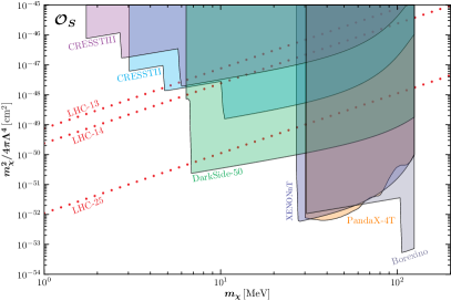
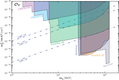
Fig. 18: The excluded regions on the $m_{\chi}^{2}/4\pi\varLambda^{4}$-$m_{\chi}$ plane for the scalar (left-panel) and the vector (right-panel) operators.

In the window of $m_{\chi}\in[\sim 10,\sim 100]\,$MeV, the absorption process can provide stronger constraints than the collider searches. Outside, the LHC search always gives stronger constraints. Between the two operators, the scalar operator receives slightly stronger bound than its vector counterpart due to a larger nucleon form factor when matching from the quark-level operator to the nucleon matrix elements.

4.2 Spin-Dependent Absorption

As demonstrated in App. B, the pseudo-scalar and axial-vector operators can induce SD interactions. Different from the axial-vector operator, the leading contribution for the pseudo-scalar operator is suppressed by an extra factor of $q/m_{A}\sim m_{\chi}/m_{A}$. In following studies, the nucleon-level matrix elements proportional to $q/m_{A}$ will be neglected except the pseudo-scalar operator. With this approximation, there are only two types of SD interactions,

$$\mathcal{O}_{SS} =\big{[}(\xi_{h_{\nu}}^{\nu})^{\dagger}\boldsymbol{s}\,\xi^{\chi}_{h_{\chi}}\big{]}\big{[}(\omega_{h_{N^{\prime}}}^{N^{\prime}})^{\dagger}\boldsymbol{s}\,\omega_{h_{N}}^{N}\big{]}\,,$$ (4.12a)

$$\mathcal{O}_{LS} =\big{[}(\xi_{h_{\nu}}^{\nu})^{\dagger}\xi^{\chi}_{h_{\chi}}\big{]}\big{[}(\omega_{h_{N^{\prime}}}^{N^{\prime}})^{\dagger}\big{(}\boldsymbol{q}\cdot\boldsymbol{s}\,\big{)}\,\omega_{h_{N}}^{N}\big{]}\,,$$ (4.12b)

where $\xi_{h_{a}}^{a}$ are the two-component spinors with helicity $h_{a}$ for the neutrino ($a=v$) and the DM ($a=\chi$) while $\omega_{h_{a}}^{a}$ are the two-component spinors with helicity $h_{a}$ for the incoming nucleon ($a=N$) and the outgoing nucleon ($a=N^{\prime}$). Using the non-relativistic expansions in App. B, the nucleon matrix elements for the pseudo-scalar and axial-vector operators can be rewritten in terms of $\mathcal{O}_{SS}$ and $\mathcal{O}_{LS}$ as,

$$\mathcal{O}^{N}_{P} =2\sqrt{2}h_{\nu}m_{\chi}F_{P}^{N}\mathcal{O}_{LS}\,,\quad\quad F_{P}^{N}=\sum_{q}\frac{F^{q/N}_{P}}{m_{q}}\,,$$ (4.13a)

$$\mathcal{O}^{N}_{A} =8\sqrt{2}m_{\chi}m_{A}F_{A}^{N}\mathcal{O}_{SS}\,,\quad\quad F_{A}^{N}=\sum_{q}F^{q/N}_{A}\,,$$ (4.13b)

where $F_{P}^{N}$ and $F_{A}^{N}$ are the nucleon form factors for the pseudo-scalar and axial-vector operators, respectively. At the nucleus level, the matrix elements of the non-relativistic operators are,

$$\mathcal{M}_{A,SS} =\sum_{N=p,n}\boldsymbol{s}_{\chi}\cdot\left\langle J,M^{\prime}\left|\boldsymbol{S}_{N}\right|J,M\right\rangle,$$ (4.14a)

$$\mathcal{M}_{A,LS} =\sum_{N=p,n}\mathbb{I}_{\chi}\;\big{[}\left\langle J,M^{\prime}\left|\boldsymbol{S}_{N}\right|J,M\right\rangle\cdot\boldsymbol{q}\big{]},$$ (4.14b)

where $\boldsymbol{s}_{\chi}$ is the DM/neutrino spin operators, and $\mathbb{I}_{\chi}$ is an identity operator in the spinor space. While $J$ and $M$ are the total and projected spin quantum numbers, $\boldsymbol{S}_{N}$ is the total nucleon spin operator defined as $\boldsymbol{S}_{p}\equiv\sum_{i=\text{ protons }}\boldsymbol{s}_{p_{i}}$ and $\boldsymbol{S}_{n}\equiv\sum_{i=\text{ neutrons }}\boldsymbol{s}_{n_{i}}$ for proton and neutron, respectively. In case of that the total spin $J=0$, the above matrix elements clearly vanishes. Some typical experiments, which contains parts of isotopes having non-zero total spin, are listed in Table 3. We will study the SD signals at these experiments.

Experiment	Target	Exposure	Isotope (Abund.)	$E_{\rm R}^{\rm th}$
XENONnT [136]	Liquid Xe	1.09 t yr	${}^{129}_{\;\;54}\mathrm{Xe}$ (26.4%) ${}^{131}_{\;\;54}\mathrm{Xe}$ (21.2%)	3 keV
PandaX-4T [144]	Liquid Xe	0.63 t yr	${}^{129}_{\;\;54}\mathrm{Xe}$ (26.4%) ${}^{131}_{\;\;54}\mathrm{Xe}$ (21.2%)	3 keV
Borexino [138]	$\mathrm{C}_{6}\mathrm{H}_{3}\left(\mathrm{CH}_{3}\right)_{3}$	817 t yr	${}^{13}_{\;\,6}\mathrm{C}$ (1.1%) ${}^{1}_{1}\mathrm{H}$ (99.985%)	500 keV
CRESST-III [145]	$\mathrm{Li}\mathrm{Al}\mathrm{O}_{2}$	2.345 kg day	${}^{6}_{3}\mathrm{Li}$ (7.5%) ${}^{7}_{3}\mathrm{Li}$ (92.5%) ${}^{27}_{13}\mathrm{Al}$ (100%)	94.1 eV
PICO-60 [146]	$\mathrm{C}_{3}\mathrm{F}_{8}$	2207 kg day	${}^{13}_{\;\,6}\mathrm{C}$ (1.1%) ${}^{19}_{\;\,9}\mathrm{F}$ (100%)	3.3 keV

Table 3: The dark matter and neutrino experiments studied here for probing the SD absorption signals.

The squared amplitudes summing over the final-state spins and averaging over the initial states are given as

$$\overline{\big{|}\mathcal{M}_{A,SS}\big{|}^{2}} =\frac{1}{2}\sum_{N,N^{\prime}}F_{4,4}^{NN^{\prime}}=\sum_{N,N^{\prime}}\frac{1}{32}\Big{[}F_{\Sigma^{\prime}}^{NN^{\prime}}(q^{2})+F_{\Sigma^{\prime\prime}}^{NN^{\prime}}(q^{2})\Big{]},$$ (4.15a)

$$\overline{\big{|}\mathcal{M}_{A,LS}\big{|}^{2}} =\sum_{N,N^{\prime}}F_{10,10}^{NN^{\prime}}=\sum_{N,N^{\prime}}\frac{q^{2}}{4}F_{\Sigma^{\prime\prime}}^{NN^{\prime}}(q^{2}).$$ (4.15b)

There is an additional factor $1/2$ due to that only left-handed neutrino can take part into the scattering. The response functions are defined as,

$$F_{4,4}^{NN^{\prime}} =\frac{1}{4(2J+1)}\sum_{M,M^{\prime}}\left\langle J,M\left|\boldsymbol{S}_{N^{\prime}}\right|J,M^{\prime}\right\rangle\left\langle J,M^{\prime}\left|\boldsymbol{S}_{N}\right|J,M\right\rangle\,,$$ (4.16a)

$$F_{10,10}^{NN^{\prime}} =\frac{1}{2J+1}\sum_{M,M^{\prime}}\left\langle J,M\left|\boldsymbol{S}_{N^{\prime}}\cdot\boldsymbol{q}\right|J,M^{\prime}\right\rangle\left\langle J,M^{\prime}\left|\boldsymbol{S}_{N}\cdot\boldsymbol{q}\right|J,M\right\rangle\,.$$ (4.16b)

For the non-relativistic operator $\mathcal{O}_{SS}$ in Eq. (4.12a), the nuclear response function can be of both the $\Sigma^{{}^{\prime}}$ and $\Sigma^{{}^{\prime\prime}}$ types as defined in Eq. (4.15), while for the operator $\mathcal{O}_{LS}$, there is only the $\Sigma^{{}^{\prime\prime}}$ response [24]. In general, these response functions are complex functions of the momentum transfer and model parameters. The explicit form of $F_{\Sigma^{\prime}}^{NN^{\prime}}$ and $F_{\Sigma^{\prime\prime}}^{NN^{\prime}}$ for some isotopes can be found in Ref. [147]. Here we simply employ the zero momentum transfer approximation where the response function $F_{10,10}^{NN^{\prime}}\propto q^{2}$ vanishes. However, with the help of following relation at the zero momentum transfer,

$$\sum_{M,M^{\prime}}\left\langle J,M\left|S_{N^{\prime},i}\right|J,M^{\prime}\right\rangle\left\langle J,M^{\prime}\left|S_{N,j}\right|J,M\right\rangle=\frac{(J+1)(2J+1)}{3J}\mathbb{S}_{N}\mathbb{S}_{N^{\prime}}\delta_{ij}\,,$$ (4.17)

where $\mathbb{S}_{N}\equiv\left\langle J,J\left|S_{N}^{z}\right|J,J\right\rangle$ are the expectation values of the nucleus spin operator for the maximal spin projection, the response functions are given as,

$$F_{4,4}^{NN^{\prime}} =\frac{J+1}{4J}\mathbb{S}_{N}\mathbb{S}_{N^{\prime}}\,,\quad\quad F_{\Sigma^{\prime}}^{NN^{\prime}}+F_{\Sigma^{\prime\prime}}^{NN^{\prime}}=\frac{4(J+1)}{J}\mathbb{S}_{N}\mathbb{S}_{N^{\prime}}\,,$$ (4.18a)

$$F_{10,10}^{NN^{\prime}} =\frac{J+1}{3J}q^{2}\mathbb{S}_{N}\mathbb{S}_{N^{\prime}}\,,\quad\quad F_{\Sigma^{\prime\prime}}^{NN^{\prime}}=\frac{4(J+1)}{3J}\mathbb{S}_{N}\mathbb{S}_{N^{\prime}}\,.$$ (4.18b)

Particularly, the response function $F_{10,10}^{NN^{\prime}}(q^{2})$ is approximately $F_{10,10}^{NN^{\prime}}(q^{2}=0)\approx q^{2}/4\,F_{\Sigma^{\prime\prime}}^{NN^{\prime}}(q^{2}=0)$ such that the $q^{2}$ dependence is factorized out. Since determining $\mathbb{S}_{N}$ requires detailed calculations within realistic nuclear models, its values found in the literature are often model dependent and sometimes differ one from another for a given nucleus. Table 4 summarizes the spin expectation values ($\mathbb{S}_{N}$) of some isotopes that will be studied in this paper.

Isotope (Abund.)	$J$	$\mathbb{S}_{p}$	$\mathbb{S}_{n}$	Ref.
${}^{1}_{1}\mathrm{H}$ (99.985%)	1/2	0.5	0	[148, 149]
${}^{6}_{3}\mathrm{Li}$ (7.5%)	1/2	0.472	0.472	[150, 145]
${}^{7}_{3}\mathrm{Li}$ (92.5%)	3/2	0.497	0.004	[151]
${}^{13}_{\,\,\,6}\mathrm{C}$ (1.1%)	1/2	$-0.009$	$-0.172$	[152]
${}^{19}_{\,\,\,9}\mathrm{F}$ (100%)	1/2	0.475	$-0.0087$	[153]
${}^{27}_{13}\mathrm{Al}$ (100%)	5/2	0.343	0.0296	[154]
${}^{129}_{\;\;54}\mathrm{Xe}$ (26.4%) ${}^{131}_{\;\;54}\mathrm{Xe}$ (21.2%)	1/2 3/2	0.0128 $-0.012$	0.300 $-0.217$	[155]

Table 4: The spin expectation values ($\mathbb{S}_{N}$) of the isotopes studied in this paper.

The readers can also find some averaged values from Ref. [24]. In the scattering rate calculation, it usually assumes that either proton or neutron takes part into the interaction. Here we consider only the nucleon which has the largest spin expectation value for the given isotopes shown in Table 4.

Including the phase space factor, the scattering rate can be written in terms of the response functions as,

$$R_{A}^{P} =\frac{N_{A}n_{\chi}m_{\chi}^{4}}{8\pi\varLambda_{P}^{4}m_{A}^{2}}\varTheta(E_{\rm R}^{0}-E_{\rm R}^{\rm th})\sum_{N,N^{\prime}=p,n}F_{P}^{N}F_{P}^{N^{\prime}}\big{[}F_{\Sigma^{\prime\prime}}^{NN^{\prime}}\big{]}\,,$$ (4.19a)

$$R_{A}^{A} =\frac{N_{A}n_{\chi}m_{\chi}^{2}}{4\pi\varLambda_{A}^{4}}\varTheta(E_{\rm R}^{0}-E_{\rm R}^{\rm th})\sum_{N,N^{\prime}=p,n}F_{A}^{N}F_{A}^{N^{\prime}}\big{[}F_{\Sigma^{\prime}}^{NN^{\prime}}+F_{\Sigma^{\prime\prime}}^{NN^{\prime}}\big{]}\,.$$ (4.19b)

The SD scattering are parameterized by using the spin structure function $S(q^{2})\equiv 4(2J+1)F_{4,4}^{NN^{\prime}}$. However, the usual spin structure function $S(q^{2})$ is somehow specific for the axial-vector matrix operator. For instance, the differential scattering rate for axial vector operator can be cast into a usual form in term of $S(q^{2})$ (apart from the phase space factors),

$$\frac{\mathrm{d}R_{T}^{A}}{\mathrm{d}E_{\mathrm{R}}}\propto\frac{N_{T}n_{\chi}m_{\chi}^{2}}{\pi(2J+1)\varLambda_{A}^{4}}F_{A}^{N}F_{A}^{N^{\prime}}S(q^{2})=\frac{N_{T}n_{\chi}m_{\chi}^{2}}{\pi\varLambda_{A}^{4}}\frac{J+1}{J}F_{A}^{N}F_{A}^{N^{\prime}}\mathbb{S}_{N}\mathbb{S}_{N^{\prime}}\frac{S(q^{2})}{S(0)}\,,$$ (4.20)

where the factor $S(0)=\mathbb{S}_{N}\mathbb{S}_{N^{\prime}}(2J+1)(J+1)/J$ can be obtained using the definition of $S(q^{2})$ given in Eq. (4.18a). Similar expressions can also be found for the tensor operator. In our case, it is better to use the response functions $F_{\Sigma^{\prime}}^{NN^{\prime}}$ and $F_{\Sigma^{\prime\prime}}^{NN^{\prime}}$ (in the limit $q^{2}\to 0$), such that the pseudo-scalar operator contribution can also studied in terms of the same response functions.

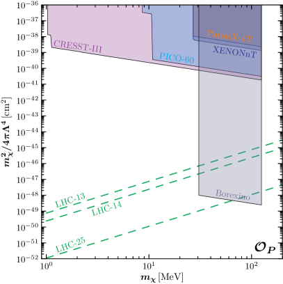
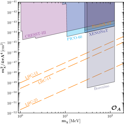
Fig. 19: The excluded regions on the $m_{\chi}^{2}/4\pi\varLambda^{4}$-$m_{\chi}$ plane with SD scatterings for the pseudo-scalar (left-panel) and the axial-vector (right-panel) operators.

The exclusion bounds for those experiments listed in Table 3 are estimated by requiring the total event number to be greater than 10. Fig. 19 shows the expected excluded regions on the $m_{\chi}^{2}/4\pi\varLambda^{4}$-$m_{\chi}$ plane. Those constraints given by the SD experiments with relatively heavier nucleus are much weaker than the LHC searches while the light nucleus target can provide stronger constraints. This is particularly true for the Borexino experiment with hydrogen with two reasons. First, the Borexino experiment has about 3 orders larger exposure as shown in Table 3. Second, for given detector mass, the nuclei (proton for the Borexino experiment) number is more than 2 orders larger than those experiment with heavy nuclei (for instance $\mathrm{Xe}$ of the PandaX and XENON). Without coherence enhancement, the SD cross section is roughly the same among the light and heavy nucleus and hence the nuclei number determines the total event rate. With these two advantages, one can see a roughly 6 orders stronger constraint on the axial-vector operator from Borexino (the right-panel of Fig. 19). For the pseudo-scalar operator (the left-panel of Fig. 19), the enhancement at the Borexino experiment is even stronger since the scattering rate is suppressed by a factor $m_{\chi}^{2}/m_{A}^{2}$ which is inversely proportional to $m^{2}_{A}$. The effect of this suppression factor also manifests itself as stronger constraint for heavier DM in the right-panel of Fig. 19, in contrast to the axial-vector case. Another interesting point is that the SD constraints can be as strong as the SI one with light nucleus since the coherence enhancement for the SI scattering is then dramatically diminished.

4.3 Absorption for the Tensor Operator

As mentioned easier, the quark-level tensor operator can induce both SI and SD interactions at the nucleon level. So the total amplitude is the sum of two contributions,

$$\mathcal{M}_{A,T}=\mathcal{M}_{A,T}^{SD}+\mathcal{M}_{A,T}^{SI}\,.$$ (4.21)

For the SD interaction induced by the first term of Eq. (4.7e), the nucleon matrix elements are dominated by the non-relativistic operator $\mathcal{O}_{SS}$ in Eq. (4.12a) according to the non-relativistic expansions in App. B, Similar to the axial-vector case in Eq. (4.14a), the scattering amplitude is given as,

$$\mathcal{M}_{A,T}^{SD}=16\sqrt{2}m_{\chi}m_{A}\sum_{N=p,n}F_{T,SD}^{N}\big{[}\boldsymbol{s}_{\chi}\cdot\left\langle J,M^{\prime}\left|\boldsymbol{S}_{N}\right|J,M\right\rangle\big{]}\,,\quad F_{T,SD}^{N}=\sum_{q}\frac{F^{q/N}_{T,0}}{m_{q}}\,.$$ (4.22)

For the SI interaction induced by the second and third terms of Eq. (4.7e), the largest contribution is given by the off-diagonal parts of the nucleon-level tensor matrix elements. The corresponding non-relativistic operator is,

$$\mathcal{O}_{L}=\big{[}h_{\nu}(\xi_{h_{\nu}}^{\nu})^{\dagger}(\boldsymbol{s}_{\chi}\cdot\boldsymbol{q})\,\xi^{\chi}_{h_{\chi}}\big{]}\mathbb{I}_{N}\,.$$ (4.23)

and the scattering amplitude is,

$$\mathcal{M}_{A,T}^{SI}=4\sqrt{2}m_{\chi}\sum_{N=p,n}F_{T,SI}^{N}C_{N}F_{SI}^{N}\big{[}\boldsymbol{s}_{\chi}\cdot\boldsymbol{q}\big{]}\delta_{M^{\prime}M}\,,\quad F_{T,SI}^{N}=\sum_{q}\frac{F^{q/N}_{T,1}+2F^{q/N}_{T,2}}{m_{q}}\,,$$ (4.24)

where $F_{SI}^{N}$ is the SI response function defined in Eq. (4.9). With two contributions to the scattering amplitude, the total average squared amplitude,

$$\overline{\big{|}\mathcal{M}_{T,L}\big{|}^{2}}=\overline{\big{|}\mathcal{M}_{T,SD}\big{|}^{2}}+\overline{\big{|}\mathcal{M}_{T,SI}\big{|}^{2}}+\overline{\mathcal{M}_{T,SD}^{\dagger}\mathcal{M}_{T,SI}+\mathcal{M}_{T,SI}^{\dagger}\mathcal{M}_{T,SD}}\,,$$ (4.25)

contains an interference term between the SI and SD interactions. Summing over the DM and neutrino helicity states, the interference can be reformed as,

$$\overline{\Re\big{\{}\mathcal{M}_{T,SD}^{\dagger}\mathcal{M}_{T,SI}\big{\}}}\propto\sum_{M}\left\langle J,M\left|\boldsymbol{q}\cdot\boldsymbol{S}_{N}\right|J,M\right\rangle\,.$$ (4.26)

Since the nuclear target is unpolarized and the momentum transfer orientation (or equivalently the DM velocity) is isotropic, this interference term would not leave any effect in the total event rate. So the total scattering rate is just incohenrent sum of the SD and SI contributions,

$$R_{A}^{T}=R_{A,SD}^{T}+R_{A,SI}^{T}\,,$$ (4.27)

where the SD and SI scattering rates are given as follows,

$$R_{A,SD}^{T} =\frac{16N_{A}n_{\chi}m_{\chi}^{2}}{\pi\varLambda_{T}^{4}}\varTheta(E_{\rm R}^{0}-E_{\rm R}^{\rm th})\sum_{N,N^{\prime}=p,n}F_{T,SD}^{N}F_{T,SD}^{N^{\prime}}\big{[}F_{\Sigma^{\prime}}^{NN^{\prime}}+F_{\Sigma^{\prime\prime}}^{NN^{\prime}}\big{]}\,,$$ (4.28a)

$$R_{A,SI}^{T} =N_{A}n_{\chi}\frac{m_{\chi}^{4}}{4\pi\varLambda_{T}m_{A}^{2}}\big{[}AF_{T,SI}^{N}F_{\rm Helm}(m_{\chi}^{2})\big{]}^{2}\varTheta(E_{\rm R}^{0}-E_{\rm R}^{\rm th})\,.$$ (4.28b)

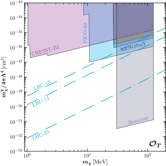
Fig. 20: The excluded regions on the $m_{\chi}^{2}/4\pi\varLambda^{4}$-$m_{\chi}$ plane with SD scatterings for the tensor operator.

The SI contribution is suppressed by a factor of $m_{\chi}^{2}/m_{A}^{2}$, similar to the pseudo-scalar contribution to the SD scattering as shown in Eq. (4.19a)). However, the SI contribution of tensor operator still has the coherency enhancement factor $A^{2}$ which is large for heavier nucleus. Comparing with the SD contribution, the SI scattering rate is roughly scaled by a factor $A^{2}m_{\chi}^{2}/m_{A}^{2}\approx m_{\chi}^{2}/m_{N}^{2}$ with the nucleus mass $m_{A}$ replaced by the nucleon mass $m_{N}$. In other words, the SI scattering on a light nuclear target needs not to be relatively much smaller. However, for the DM mass window $m_{\chi}\lesssim 100\,$MeV at the direct detection experiments, the net enhancement is negligible with $m_{\chi}\ll m_{N}$. Fig. 20 shows the expected excluded regions for the tensor operator on the $m_{\chi}^{2}/4\pi\varLambda^{4}$-$m_{\chi}$ plane. The current LHC bound has covered almost all the constraints given by the SD experiments with heavy nucleus. However, the bound obtained with light nucleus at the Borexino experiment is still the most promising channel of detecting the absorption signal.

5 Conclusion

Starting from the quark-level fermionic absorption operators, we study for the first time their sensitivities at the LHC and compare with the constraints from the DM direct detection as well as neutrino experiments. In addition to covering the light DM scenarios, the collider search applies to dark sector fermions in general with much larger mass range extending up to the TeV scale. Even for DM with typical mass below $\mathcal{O}(100)$ MeV, the LHC searches can provide better sensitivities although the identification still requires direct detection experiments that has unique recoil energy spectrum. While for scalar and vector operators, the DM direct detection experiments with heavy nuclei target has much better sensitivities, the remaining pseudo-scalar, axial-vector, and tensor operators has much better sensitivities at neutrino experiments with light nuclei. It is also interesting to observe that the tensor operator can have comparable contributions from both the SI and SD scattering.

Appendix A Nucleon Form Factors

For completeness we list all the nucleon form factors needed in our calculations of the DM-nucleon scattering cross sections. We follow the parameterizations in Ref. [56] and study only the leading order corrections at the zero momentum transfer limit $q^{2}\approx 0$. Imposing the isospin symmetry, most of the form factors $F_{\varGamma,\ldots}^{q/N}$ are given for proton, i.e., $N=p$, while the neutron ones can be obtained by exchanging $p\to n$ and $u\leftrightarrow d$. The small differences between $F_{\varGamma,\ldots}^{q/p}$ and $F_{\varGamma,\ldots}^{q/n}$ can then be ignored.

A.1 Scalar Current

The scalar form factors $F_{S}^{q/N}$ are conventionally referred as the nuclear sigma terms. In the zero momentum transfer approximation,

$$F_{S}^{q/N}(q^{2}=0)=\sigma_{q}^{N}\,.$$ (A.1)

The matrix elements of the $u$ and $d$ quarks are related to the pion-nucleon sigma term, $\sigma_{\pi N}=\langle N|\overline{m}(\bar{u}u+\bar{d}d)$ with $\overline{m}=(m_{u}+m_{d})/2$. There are several methods to obtain the experimental fits of $\sigma_{\pi N}$, for example $\sigma_{\pi N}=50\pm 15\,{\rm MeV}$ [56]. And the corresponding sigma terms are [56, 130],

$$\sigma_{u}^{p}=(17\pm 5)\,\mathrm{MeV}\,, \sigma_{d}^{p}=(32\pm 10)\,\mathrm{MeV}\,,$$ (A.2)

$$\sigma_{u}^{n}=(15\pm 5)\,\mathrm{MeV}\,, \sigma_{d}^{n}=(36\pm 10)\,\mathrm{MeV}\,.$$

For the strange quark, the average of lattice QCD determinations gives [157, 159, 158, 56],

$$\sigma_{s}^{p}=\sigma_{s}^{n}=(41.3\pm 7.7)\,\mathrm{MeV}\,.$$ (A.3)

The matching between the quark- and hadron-level matrix elements requires also inputting the quark masses ($m_{u}=2.14\pm 8$ MeV, $m_{d}=4.70\pm 5$ MeV, and $m_{s}/\bar{m}=27.5\pm 0.3$) since the matching coefficients are proportional to $F_{S}^{q/N}(0)/m_{q}$. Then we can find

$$\left[\sum_{q=u,d,s}\frac{F_{S}^{q/N}(q^{2}=0)}{m_{q}}\right]^{2}=\begin{cases}15.2&N=p,\\[2.84526pt] 15.1&N=n.\end{cases}$$ (A.4)

The difference between the matching coefficients for proton and neutron is negligible.

A.2 Pseudo-Scalar Current

The pseudo-scalar current can receive contributions from the light pseudo-scalar meson exchange and hence its amplitude has pole structures at the meson mass points [56]. For small momenta exchange, the form factors expands as,

$$F_{P}^{q/N}\left(q^{2}\right)=\frac{m_{N}^{2}}{m_{\pi}^{2}-q^{2}}a_{P,\pi}^{q/N}+\frac{m_{N}^{2}}{m_{\eta}^{2}-q^{2}}a_{P,\eta}^{q/N}+\cdots\,.$$ (A.5)

The residua of the poles are given by

$$\frac{a_{P,\pi}^{u/p}}{m_{u}} =-\frac{a_{P,\pi}^{d/p}}{m_{d}}=\frac{B_{0}}{m_{N}}g_{A}\,,\quad\frac{a_{P,\pi}^{s/p}}{m_{s}}=0\,,$$ (A.6a)

$$\frac{a_{P,\eta}^{u/p}}{m_{u}} =\frac{a_{P,\eta}^{d/p}}{m_{d}}=-\frac{1}{2}\frac{a_{P,\eta}^{s/p}}{m_{s}}=\frac{B_{0}}{3m_{N}}\left(\Delta u_{p}+\Delta d_{p}-2\Delta s_{p}\right)\,.$$ (A.6b)

The coefficients for the neutron case can be obtained through the replacement $p\to n$ and $u\leftrightarrow d$. In the isospin limit,

$$\Delta u_{n}=\Delta d_{p}\equiv\Delta u\,,\quad\Delta u_{n}=\Delta d_{p}\equiv\Delta d\,,\quad\Delta s_{n}=\Delta s_{p}\equiv\Delta s\,.$$ (A.7)

The iso-vector combination can be precisely determined from the nuclear $\beta$ decay [160],

$$\Delta u-\Delta d=g_{A}=1.2723(23).$$ (A.8)

In the $\overline{\mathrm{MS}}$ scheme at $Q=2\mathrm{GeV}$, the averages of lattice QCD results give $\Delta u+\Delta d=0.521(53)$ [161] and $\Delta s=-0.031(5)$. The combination of these results gives [161],

$$\Delta u=0.897(27),\quad\Delta d=-0.376(27),\quad\Delta s=-0.031(5).$$ (A.9)

Moreover, $B_{0}$ is a ChPT (chiral perturbation theory) constant related to the quark condensate and up to the order $\mathcal{O}\left(m_{q}\right)$ it is given by $\langle\bar{q}q\rangle\simeq-f^{2}B_{0}$. At the leading order, the quark condensate gives $f=f_{\pi}$, with $f_{\pi}$ being the pion decay constant [162]. Then one has $B_{0}=2.666(57)\,\mathrm{GeV}$ at the scale $\mu=2\,\mathrm{GeV}$. Then one can find,

$$\sum_{q=u,d,s}\frac{F_{P}^{q/p}(0)}{m_{q}}\approx 6.43.$$ (A.10)

A.3 Vector Currents

For the vector current, the matrix elements at the hadron level are parameterized by two sets of form factors $F_{1}^{q/N}\left(q^{2}\right)$ and $F_{2}^{q/N}\left(q^{2}\right)$. For matching at the leading order only their values evaluated at $q^{2}=0$ are necessary. In the zero momentum transfer limit, the vector currents just count the number of valence quarks in the nucleon. Hence, the normalizations of the proton form factors are,

$$F_{1}^{u/p}(0)=2,\quad F_{1}^{d/p}(0)=1,\quad F_{1}^{s/p}(0)=0\,.$$ (A.11)

The form factors $F_{2}^{q/N}(0)$ as defined in Eq. (4.7c) describe the quark contributions to the nucleon anomalous magnetic moments,

$$a_{p} =\frac{2}{3}F_{2}^{u/p}(0)-\frac{1}{3}F_{2}^{d/p}(0)-\frac{1}{3}F_{2}^{s/p}(0)\approx 1.793\,,$$ (A.12a)

$$a_{n} =\frac{2}{3}F_{2}^{u/n}(0)-\frac{1}{3}F_{2}^{d/n}(0)-\frac{1}{3}F_{2}^{s/n}(0)\approx-1.913\,.$$ (A.12b)

The strange magnetic moment is given by [164, 163],

$$F_{2}^{s/p}(0)=-0.064(17)\,.$$ (A.13)

Then one can obtain,

$$F_{2}^{u/p}(0)=1.609(17)\,,\quad F_{2}^{d/p}(0)=-2.097(17)\,.$$ (A.14)

Using these results we have,

$$\sum_{q=u,d,s}F_{1}^{q/p}(0)=3,\qquad\sum_{q=u,d,s}F_{2}^{q/p}(0)=-0.552.$$ (A.15)

A.4 Axial-vector current

For the axial-vector operator, the hadron-level matrix elements are parametrized by two sets of form factors, $F_{A}^{q/N}\left(q^{2}\right)$ and $F_{P^{\prime}}^{q/N}\left(q^{2}\right)$. At the leading order, only $F_{A}^{q/N}(0)$ and the light meson pole contribution $F_{P^{\prime}}^{q/N}\left(q^{2}\right)$ are necessary for our calculations. The axial-vector form factor at zero momentum transfer can be calculated from the matrix elements parameterization $2m_{p}s^{\mu}\Delta q_{\mu}=\langle p|\bar{q}\gamma_{\mu}\gamma_{5}q|p\rangle_{Q}$ at scale $Q$ with $s^{\mu}$ being the proton polarization vector,

$$F_{A}^{q/p}(0)=\Delta q_{p}\,.$$ (A.16)

For the light meson parts, it can be expanded as,

$$F_{P^{\prime}}^{q/N}\left(q^{2}\right)=\frac{m_{N}^{2}}{m_{\pi}^{2}-q^{2}}a_{P^{\prime},\pi}^{q/N}+\frac{m_{N}^{2}}{m_{\eta}^{2}-q^{2}}a_{P^{\prime},\eta}^{q/N}+\cdots\,.$$ (A.17)

And the residua of the pion- and eta-pole contributions to $F_{P^{\prime}}^{q/N}$ are given as,

$$a_{P^{\prime},\pi}^{u/p} =-a_{P^{\prime},\pi}^{d/p}=2g_{A}\,,\quad a_{P^{\prime},\pi}^{s/p}=0\,,$$ (A.18a)

$$a_{P^{\prime},\eta}^{u/p} =a_{P^{\prime},\eta}^{d/p}=-\frac{1}{2}a_{P^{\prime},\eta}^{s/p}=\frac{2}{3}\left(\Delta u_{p}+\Delta d_{p}-2\Delta s_{p}\right)\,.$$ (A.18b)

Using these results we have,

$$\sum_{q=u,d,s}F_{A}^{q/p}(0)=0.49\,,\qquad\sum_{q=u,d,s}F_{P^{\prime}}^{q/p}(0)\approx-3.15\times 10^{-15}\,.$$ (A.19)

A.5 Tensor Operator

The hadron-level matrix elements of the tensor operator are parameterized by three form factors, $F_{T,0}^{q/N}\left(q^{2}\right)$, $F_{T,1}^{q/N}\left(q^{2}\right)$, and $F_{T,2}^{q/N}\left(q^{2}\right)$. They are related to the generalized tensor form factors [166, 165],

$$F_{T,0}^{q/N}\left(q^{2}\right)=m_{q}A_{T,10}^{q/N}\left(q^{2}\right),\quad F_{T,1}^{q/N}\left(q^{2}\right)=-m_{q}B_{T,10}^{q/N}\left(q^{2}\right),\quad F_{T,2}^{q/N}\left(q^{2}\right)=\frac{m_{q}}{2}\tilde{A}_{T,10}^{q/N}\left(q^{2}\right).$$ (A.20)

At the leading order, only $F_{T,0}^{q/N}(0)$ and $F_{T,1}^{q/N}(0)$ appear. The value of $F_{T,0}^{q/N}(0)$ is quite well determined and is usually expressed in terms of $A_{T,10}^{q/p}(0)\equiv g_{T}^{q}$ (with $A_{T,10}^{u(d)/p}=$ $A_{T,10}^{d(u)/n}$ and $A_{T,10}^{s/p}=A_{T,10}^{s/n}$ in the isospin limit). The tensor charges $g_{T}^{q}$ are related to the transversity structure functions $\delta q_{N}(x,\mu)$ by $g_{T}^{q}(\mu)=$ $\int_{-1}^{1}dx\delta q_{N}(x,\mu)$. The lattice calculations in the $\overline{\mathrm{MS}}$ scheme at $\mu=2\mathrm{GeV}$, including both connected and disconnected contributions gives [168, 167],

$$g_{T}^{u}=0.794\pm 0.015,\quad g_{T}^{d}=-0.204\pm 0.008,\quad g_{T}^{s}=(3.2\pm 8.6)\cdot 10^{-4}$$ (A.21)

The other two form factors at zero momentum transfer, $F_{T,1}^{q/N}(0)$ and $F_{T,2}^{q/N}(0)$, are less well determined. The constituent quark model gives [169],

$$B_{T,10}^{u/p}(0)\approx 3.0\,,\quad\tilde{A}_{T,10}^{u/p}\approx-0.50\,,\quad B_{T,10}^{d/p}(0)\approx 0.24\,,\quad\tilde{A}_{T,10}^{d/p}\approx 0.46\,.$$ (A.22)

For the $s$-quark component, we have following rough estimates,

$$-0.2\lesssim B_{T,10}^{s/p}(0)\,,\;\tilde{A}_{T,10}^{s/p}(0)\lesssim 0.2$$ (A.23)

We find the form factors are insensitive to the values of $B_{T,10}^{s/p}(0)$ and $\tilde{A}_{T,10}^{s/p}(0)$. Using these results we have,

$$\sum_{q=u,d,s}\frac{F_{T,0}^{q/p}(0)}{m_{q}}\approx 0.59,\quad\sum_{q=u,d,s}\frac{F_{T,1}^{q/p}(0)}{m_{q}}\in\big{[}-2.96,\,-2.56\big{]}\,,\quad\sum_{q=u,d,s}\frac{F_{T,2}^{q/p}(0)}{m_{q}}\in\big{[}-0.12,\,0.08\big{]}\,,$$

where the boundaries correspond to lower and upper limits of $B_{T,10}^{s/p}(0)$ and $\tilde{A}_{T,10}^{s/p}(0)$. Our calculations use the lower boundaries to estimate the hadron-level cross sections of the DM scattering off nucleons.

Appendix B Non-Relativistic Expansion

The non-relativistic expansion of the usual DM-nucleon interaction operators can be found in the Ref. [24] and references within. In our case, since the neutrino is always relativistic, we revisit the the non-relativistic expansions of both the nucleon pair and DM-neutrino pair bilinears. For completeness, we give our conventions for the spinor wave functions in the Dirac representation as well as their non-relativistic expansions [170]. In the Dirac representation, the Dirac matrixes are,

$$\gamma^{0}_{D} = \left(\begin{array}[]{cc}1&0\\ 0&-1\end{array}\right)\,,\;\;\;\vec{\gamma}_{D}=\left(\begin{array}[]{cc}0&\vec{\sigma}\\ -\vec{\sigma}&0\end{array}\right)\,,\;\;\;\gamma^{5}_{D}=\left(\begin{array}[]{cc}0&1\\ 1&0\end{array}\right)\,.$$ (B.7)

The free particle solutions of the Dirac equation then has large and small components,

$$\frac{u_{D}(\vec{p}_{1},s)}{\sqrt{E+m}}=\left(\begin{array}[]{c}\xi_{s}\\[8.53581pt] \dfrac{\vec{\sigma}\cdot\vec{p}_{1}}{E+m}\xi_{s}\end{array}\right)\,,\;\;\;\frac{v_{D}(\vec{p}_{2},r)}{\sqrt{E+m}}=\left(\begin{array}[]{c}r\dfrac{\vec{\sigma}\cdot\vec{p}_{2}}{E+m}\xi_{-r}\\[8.53581pt] r\xi_{-r}\end{array}\right)\,,$$ (B.12)

and

$$\frac{\overline{u_{D}}(\vec{p}_{1},s)}{\sqrt{E+m}}=\left(\begin{array}[]{cc}\xi_{s}^{\dagger}&\xi_{s}^{\dagger}\dfrac{-\vec{\sigma}\cdot\vec{p}_{1}}{E+m}\end{array}\right)\,,\;\;\;\frac{\overline{v_{D}}(\vec{p}_{2},r)}{\sqrt{E+m}}=\left(\begin{array}[]{cc}r\xi_{-r}^{\dagger}\dfrac{\vec{\sigma}\cdot\vec{p}_{2}}{E+m}\quad\quad-r\xi_{-r}^{\dagger}\end{array}\right)\,,$$ (B.15)

where $\xi_{s}$ are eigenstates of the helicity operators $\vec{\sigma}\cdot\vec{p}/|\vec{p}|$ with eigenvalue $s=\pm 1$. The two-component spinors can be explicitly written in terms of the zenith ($\theta$) and azimuthal ($\phi$) angles,

$$\xi_{+}=\left(\begin{array}[]{c}\cos(\theta/2)\\ e^{i\phi}\sin(\theta/2)\end{array}\right)\,,\;\;\;\xi_{-}=\left(\begin{array}[]{c}-e^{-i\phi}\sin(\theta/2)\\ \cos(\theta/2)\end{array}\right)\,.$$ (B.20)

We can easily check that $\sum_{s=\pm}\xi_{s}\xi_{s}^{\dagger}=\mathbb{I}$. The spinor wave functions and the Dirac gamma matrices in the Dirac representation are related to the ones in the chiral representation by the following unitary transformation,

$$\psi_{D}=U_{D}\psi U_{D}^{-1}\,,\;\;\;\gamma^{\mu}_{D}=U_{D}\gamma_{C}^{\mu}U_{D}^{-1}\,,\;\;\;U_{D}=\frac{1}{\sqrt[]{2}}\left(\begin{array}[]{cc}1&1\\ -1&1\end{array}\right)\,.$$ (B.23)

Using these wave functions, we can easily find the non-relativistic expansions of the bilinears of the nuclear pair system, and also the DM-neutrino system. For the nuclear bilinears we have,

$$\overline{u}^{N^{\prime}}_{h_{N^{\prime}}}u^{N}_{h_{N}} \stackrel{{\scriptstyle\mathrm{NR}}}{{=}}2m_{\mathrm{N}}\,(\omega_{h_{N^{\prime}}}^{N^{\prime}})^{\dagger}\omega_{h_{N}}^{N},$$ (B.24a)

$$\overline{u}^{N^{\prime}}_{h_{N^{\prime}}}(i\gamma^{5})u^{N}_{h_{N}} \stackrel{{\scriptstyle\mathrm{NR}}}{{=}}-i(\omega_{h_{N^{\prime}}}^{N^{\prime}})^{\dagger}\big{(}\boldsymbol{q}\cdot\boldsymbol{\sigma}\big{)}\omega_{h_{N}}^{N},$$ (B.24b)

$$\overline{u}^{N^{\prime}}_{h_{N^{\prime}}}\gamma^{\mu}u^{N}_{h_{N}} \stackrel{{\scriptstyle\mathrm{NR}}}{{=}}(\omega_{h_{N^{\prime}}}^{N^{\prime}})^{\dagger}\left[\begin{array}[]{cc}2m_{\mathrm{N}}\mathbb{I},&\quad\boldsymbol{p}\mathbb{I}-i\boldsymbol{q}\times\boldsymbol{\sigma}\end{array}\right]\omega_{h_{N}}^{N}\,,$$ (B.24d)

$$\overline{u}^{N^{\prime}}_{h_{N^{\prime}}}\gamma^{\mu}\gamma_{5}u^{N}_{h_{N}} \stackrel{{\scriptstyle\mathrm{NR}}}{{=}}(\omega_{h_{N^{\prime}}}^{N^{\prime}})^{\dagger}\left[\begin{array}[]{cc}\boldsymbol{p}\cdot\boldsymbol{\sigma}\,,&\quad 2m_{\mathrm{N}}\boldsymbol{\sigma}\end{array}\right]\omega_{h_{N}}^{N}\,,$$ (B.24f)

$$\overline{u}^{N^{\prime}}_{h_{N^{\prime}}}\sigma^{\mu\nu}u^{N}_{h_{N}} \stackrel{{\scriptstyle\mathrm{NR}}}{{=}}(\omega_{h_{N^{\prime}}}^{N^{\prime}})^{\dagger}\left[\begin{array}[]{cc}0&\quad i\boldsymbol{q}\mathbb{I}+\boldsymbol{p}\times\boldsymbol{\sigma}\\ -i\boldsymbol{q}\mathbb{I}-\boldsymbol{p}\times\boldsymbol{\sigma}&\quad 2m_{\rm N}\varepsilon_{ijk}\boldsymbol{\sigma}_{k}\end{array}\right]\omega_{h_{N}}^{N},$$ (B.24i)

where we have used the abbreviated notations $u^{N}_{h_{N}}=u_{N}(\boldsymbol{p}_{i},h_{N})$ and $\overline{u}^{N^{\prime}}_{h_{N^{\prime}}}=\overline{u}_{N^{\prime}}(\boldsymbol{p}_{f},h_{N^{\prime}})$, and the total and relative momentum are defined as $\boldsymbol{p}=\boldsymbol{p}_{f}+\boldsymbol{p}_{i}$ and $\boldsymbol{q}=\boldsymbol{p}_{f}-\boldsymbol{p}_{i}$, respectively. Similarly for the DM-neutrino system, the corresponding wave functions are given as,

$$\frac{\overline{u_{D}}(\vec{p}_{\nu},h_{\nu})}{\sqrt{E_{\nu}}}=\left(\begin{array}[]{cc}\xi_{h_{\nu}}^{\dagger}&-h_{\nu}\,\xi_{h_{\nu}}^{\dagger}\end{array}\right),\qquad\frac{u_{D}(\vec{p}_{\chi},h_{\chi})}{\sqrt{2m_{\chi}}}=\left(\begin{array}[]{c}\xi_{h_{\chi}}\\ \dfrac{\vec{\sigma}\cdot\vec{p}_{\chi}}{2m_{\chi}}\xi_{h_{\chi}}\end{array}\right)\,.$$ (B.25)

Please note that the neutrino can only be left handed, i.e., $h_{\nu}=-1$. After similar straightforward calculations, one can find following non-relativistic expressions of the various bilinears,

$$\overline{u}^{\nu}_{h_{\nu}}u^{\chi}_{h_{\chi}} \stackrel{{\scriptstyle\mathrm{NR}}}{{=}}\sqrt{2m_{\chi}E_{\nu}}(\xi_{h_{\nu}}^{\nu})^{\dagger}\xi_{h_{\chi}}^{\chi},$$ (B.26a)

$$\overline{u}^{\nu}_{h_{\nu}}(i\gamma^{5})u^{\chi}_{h_{\chi}} \stackrel{{\scriptstyle\mathrm{NR}}}{{=}}-is_{2}\sqrt{2m_{\chi}E_{\nu}}(\xi_{h_{\nu}}^{\nu})^{\dagger}\xi_{h_{\chi}}^{\chi},$$ (B.26b)

$$\overline{u}^{\nu}_{h_{\nu}}\gamma^{\mu}u^{\chi}_{h_{\chi}} \stackrel{{\scriptstyle\mathrm{NR}}}{{=}}\sqrt{2m_{\chi}E_{\nu}}(\xi_{h_{\nu}}^{\nu})^{\dagger}\left[\begin{array}[]{cc}\mathbb{I}\,,&\quad h_{\nu}\boldsymbol{\sigma}\end{array}\right]\xi_{h_{\chi}}^{\chi},$$ (B.26d)

$$\overline{u}^{\nu}_{h_{\nu}}\gamma^{\mu}\gamma_{5}u^{\chi}_{h_{\chi}} \stackrel{{\scriptstyle\mathrm{NR}}}{{=}}\sqrt{2m_{\chi}E_{\nu}}(\xi_{h_{\nu}}^{\nu})^{\dagger}\left[\begin{array}[]{cc}h_{\nu}\mathbb{I}\,,&\quad\boldsymbol{\sigma}\end{array}\right]\xi_{h_{\chi}}^{\chi},$$ (B.26f)

$$\overline{u}^{\nu}_{h_{\nu}}\sigma^{\mu\nu}u^{\chi}_{h_{\chi}} \stackrel{{\scriptstyle\mathrm{NR}}}{{=}}\sqrt{2m_{\chi}E_{\nu}}(\xi_{h_{\nu}}^{\nu})^{\dagger}\left[\begin{array}[]{cc}0&\quad-ih_{\nu}\boldsymbol{\sigma}\\ ih_{\nu}\boldsymbol{\sigma}&\quad-\boldsymbol{\sigma}\end{array}\right]\xi_{h_{\chi}}^{\chi},$$ (B.26i)

where $\overline{u}^{\nu}_{h_{\nu}}\equiv\overline{u_{\nu}}(\vec{p}_{\nu},h_{\nu})$ and $u^{\chi}_{h_{\chi}}=u_{\chi}(\vec{p}_{\chi},h_{\chi})$.

References

- [1] G. Bertone, D. Hooper, and J. Silk, “Particle dark matter: Evidence, candidates and constraints,” Phys. Rept. 405 (2005) 279–390, [arXiv:hep-ph/0404175].
- [2] B.-L. Young, “A survey of dark matter and related topics in cosmology,” Front. Phys. (Beijing) 12 no. 2, (2017) 121201. [Erratum: Front.Phys.(Beijing) 12, 121202 (2017)].
- [3] A. Arbey and F. Mahmoudi, “Dark matter and the early Universe: a review,” Prog. Part. Nucl. Phys. 119 (2021) 103865, [arXiv:2104.11488 [hep-ph]].
- [4] M. Fairbairn, “Galactic Anomalies and Particle Dark Matter,” Symmetry 14 no. 4, (2022) 812.
- [5] L. Roszkowski, E. M. Sessolo, and S. Trojanowski, “WIMP dark matter candidates and searches—current status and future prospects,” Rept. Prog. Phys. 81 no. 6, (2018) 066201, [arXiv:1707.06277 [hep-ph]].
- [6] P. F. de Salas and A. Widmark, “Dark matter local density determination: recent observations and future prospects,” Rept. Prog. Phys. 84 no. 10, (2021) 104901, [arXiv:2012.11477 [astro-ph.GA]].
- [7] F. Chadha-Day, J. Ellis, and D. J. E. Marsh, “Axion dark matter: What is it and why now?,” Sci. Adv. 8 no. 8, (2022) abj3618, [arXiv:2105.01406 [hep-ph]].
- [8] S. Heinemeyer and C. Muñoz, “Dark Matter in Supersymmetry,” Universe 8 no. 8, (2022) 427.
- [9] C. R. Argüelles, E. A. Becerra-Vergara, J. A. Rueda, and R. Ruffini, “Fermionic Dark Matter: Physics, Astrophysics, and Cosmology,” Universe 9 no. 4, (2023) 197, [arXiv:2304.06329 [astro-ph.GA]].
- [10] A. Capolupo, A. Quaranta, and R. Serao, “Field Mixing in Curved Spacetime and Dark Matter,” Symmetry 15 no. 4, (2023) 807.
- [11] J. M. Gaskins, “A review of indirect searches for particle dark matter,” Contemp. Phys. 57, no.4, 496-525 (2016) [arXiv:1604.00014 [astro-ph.HE]].
- [12] R. K. Leane, “Indirect Detection of Dark Matter in the Galaxy,” in 3rd World Summit on Exploring the Dark Side of the Universe, pp. 203–228. 2020. [arXiv:2006.00513 [hep-ph]].
- [13] T. R. Slatyer, “Les Houches Lectures on Indirect Detection of Dark Matter,” SciPost Phys. Lect. Notes 53 (2022) 1, [arXiv:2109.02696 [hep-ph]].
- [14] J. de Dios Zornoza, “Review on Indirect Dark Matter Searches with Neutrino Telescopes,” Universe 7 no. 11, (2021) 415.
- [15] H. C. Das, A. Kumar, B. Kumar, and S. K. Patra, “Dark Matter Effects on the Compact Star Properties,” Galaxies 10 no. 1, (2022) 14, [arXiv:2112.14198 [astro-ph.HE]].
- [16] R. Brito, S. Chakrabarti, S. Clesse, C. Dvorkin, J. Garcia-Bellido, J. Meyers, K. K. Y. Ng, A. L. Miller, S. Shandera and L. Sun, “Snowmass2021 Cosmic Frontier White Paper: Probing dark matter with small-scale astrophysical observations,” [arXiv:2203.15954 [hep-ph]].
- [17] M. Hütten and D. Kerszberg, “TeV Dark Matter Searches in the Extragalactic Gamma-ray Sky,” Galaxies 10 no. 5, (2022) 92, [arXiv:2208.00145 [astro-ph.HE]].
- [18] M. de Laurentis, I. De Martino, and R. Della Monica, “The Galactic Center as a laboratory for theories of gravity and dark matter,” Rept. Prog. Phys. 86 no. 10, (2023) 104901, [arXiv:2211.07008 [astro-ph.GA]].
- [19] T. Marrodán Undagoitia and L. Rauch, “Dark matter direct-detection experiments,” J. Phys. G 43 no. 1, (2016) 013001, [arXiv:1509.08767 [physics.ins-det]].
- [20] J. Liu, X. Chen, and X. Ji, “Current status of direct dark matter detection experiments,” Nature Phys. 13 no. 3, (2017) 212–216, [arXiv:1709.00688 [astro-ph.CO]].
- [21] M. Schumann, “Direct Detection of WIMP Dark Matter: Concepts and Status,” J. Phys. G 46 no. 10, (2019) 103003, [arXiv:1903.03026 [astro-ph.CO]].
- [22] S. Cebrián, “The Role of Small Scale Experiments in the Direct Detection of Dark Matter,” Universe 7 no. 4, (2021) 81, [arXiv:2103.16191 [astro-ph.IM]].
- [23] J. Billard et al., “Direct detection of dark matter—APPEC committee report*,” Rept. Prog. Phys. 85 no. 5, (2022) 056201, [arXiv:2104.07634 [hep-ex]].
- [24] E. Del Nobile, “The Theory of Direct Dark Matter Detection: A Guide to Computations,” [arXiv:2104.12785 [hep-ph]].
- [25] M. Misiaszek and N. Rossi, “Direct Detection of Dark Matter: A Critical Review,” Symmetry 16 no. 2, (2024) 201, [arXiv:2310.20472 [hep-ph]].
- [26] F. Kahlhoefer, “Review of LHC Dark Matter Searches,” Int. J. Mod. Phys. A 32 no. 13, (2017) 1730006, [arXiv:1702.02430 [hep-ph]].
- [27] B. Penning, “The pursuit of dark matter at colliders—an overview,” J. Phys. G 45 no. 6, (2018) 063001, [arXiv:1712.01391 [hep-ex]].
- [28] A. Boveia and C. Doglioni, “Dark Matter Searches at Colliders,” Ann. Rev. Nucl. Part. Sci. 68 (2018) 429–459, [arXiv:1810.12238 [hep-ex]].
- [29] J. M. Lorenz, “Supersymmetry and the collider Dark Matter picture,” Mod. Phys. Lett. A 34 no. 30, (2019) 1930005, [arXiv:1908.09672 [hep-ex]].
- [30] S. Argyropoulos, O. Brandt, and U. Haisch, “Collider Searches for Dark Matter through the Higgs Lens,” Symmetry 13 no. 12, (2021) 2406, [arXiv:2109.13597 [hep-ph]].
- [31] P. Ilten, N. Tran, P. Achenbach, A. Ariga, T. Ariga, M. Battaglieri, J. Bian, P. Bisio, A. Celentano and M. Citron, et al. [Snowmass 2021] “Experiments and Facilities for Accelerator-Based Dark Sector Searches,” [arXiv:2206.04220 [hep-ex]].
- [32] G. Krnjaic, N. Toro, A. Berlin, B. Batell, N. Blinov, L. Darme, P. DeNiverville, P. Harris, C. Hearty and M. Hostert, et al. “A Snowmass Whitepaper: Dark Matter Production at Intensity-Frontier Experiments,” [arXiv:2207.00597 [hep-ph]].
- [33] A. Bouquet, P. Salati, and J. Silk, “-Ray Lines as a Probe for a Cold Dark Matter Halo,” Phys. Rev. D 40 (1989) 3168.
- [34] E. A. Baltz and L. Bergstrom, “Detection of leptonic dark matter,” Phys. Rev. D 67 (2003) 043516, [arXiv:hep-ph/0211325].
- [35] X.-J. Bi, X.-G. He, and Q. Yuan, “Parameters in a class of leptophilic models from PAMELA, ATIC and FERMI,” Phys. Lett. B 678 (2009) 168–173, [arXiv:0903.0122 [hep-ph]].
- [36] A. Ibarra, A. Ringwald, D. Tran, and C. Weniger, “Cosmic Rays from Leptophilic Dark Matter Decay via Kinetic Mixing,” JCAP 08 (2009) 017, [arXiv:0903.3625 [hep-ph]].
- [37] I. John and T. Linden, “Cosmic-Ray Positrons Strongly Constrain Leptophilic Dark Matter,” JCAP 12 (2021) 007, [arXiv:2107.10261 [astro-ph.HE]].
- [38] I. Reis, E. Moulin, A. Viana, and V. P. Goncalves, “Sensitivity to sub-GeV dark matter from cosmic-ray scattering with very-high-energy gamma-ray observatories,” [arXiv:2403.09343 [hep-ph]].
- [39] J. A. Dror, G. Elor, and R. Mcgehee, “Directly Detecting Signals from Absorption of Fermionic Dark Matter,” Phys. Rev. Lett. 124 no. 18, (2020) 18, [arXiv:1905.12635 [hep-ph]].
- [40] J. A. Dror, G. Elor, and R. Mcgehee, “Absorption of Fermionic Dark Matter by Nuclear Targets,” JHEP 02 (2020) 134, [arXiv:1908.10861 [hep-ph]].
- [41] T. Li, J. Liao, and R.-J. Zhang, “Dark magnetic dipole property in fermionic absorption by nucleus and electrons,” JHEP 05 (2022) 071, [arXiv:2201.11905 [hep-ph]].
- [42] PandaX Collaboration, L. Gu et al., “First Search for the Absorption of Fermionic Dark Matter with the PandaX-4T Experiment,” Phys. Rev. Lett. 129 no. 16, (2022) 161803, [arXiv:2205.15771 [hep-ex]].
- [43] Majorana Collaboration, I. J. Arnquist et al., “Exotic Dark Matter Search with the Majorana Demonstrator,” Phys. Rev. Lett. 132 no. 4, (2024) 041001, [arXiv:2206.10638 [hep-ex]].
- [44] CDEX Collaboration, W. H. Dai et al., “Exotic Dark Matter Search with the CDEX-10 Experiment at China’s Jinping Underground Laboratory,” Phys. Rev. Lett. 129 no. 22, (2022) 221802, [arXiv:2209.00861 [hep-ex]].
- [45] Kai Ma, “Signatures of Four Fermion Contact Couplings of a Dark Fermion and an Electron at Hadron Collider,” [arXiv:2404.06419 [hep-ph]].
- [46] Shao-Feng Ge and Oleg Titov, “Incoherent Fermionic Dark Matter Absorption with Nucleon Fermi Motion,” [arXiv:2405.05728 [hep-ph]].
- [47] J. A. Dror, G. Elor, R. McGehee, and T.-T. Yu, “Absorption of sub-MeV fermionic dark matter by electron targets,” Phys. Rev. D 103 no. 3, (2021) 035001, Erratum: Phys.Rev.D 105, 119903 (2022) [arXiv:2011.01940 [hep-ph]].
- [48] Shao-Feng Ge, Xiao-Gang He, Xiao-Dong Ma, and Jie Sheng, “Revisiting the fermionic dark matter absorption on electron target,” JHEP 05 (2022) 191, [arXiv:2201.11497 [hep-ph]].
- [49] PandaX Collaboration, D. Zhang et al., “Search for Light Fermionic Dark Matter Absorption on Electrons in PandaX-4T,” Phys. Rev. Lett. 129 no. 16, (2022) 161804, [arXiv:2206.02339 [hep-ex]].
- [50] EXO-200 Collaboration, S. A. Kharusi et al., “Search for MeV electron recoils from dark matter in EXO-200,” Phys. Rev. D 107 no. 1, (2023) 012007, [arXiv:2207.00897 [hep-ex]].
- [51] Shao-Feng Ge, Kai Ma, Xiao-Dong Ma, and Jie Sheng, “Associated production of neutrino and dark fermion at future lepton colliders,” JHEP 11 (2023) 190, [arXiv:2306.00657 [hep-ph]].
- [52] CDEX Collaboration, J. X. Liu et al., “First Search for Light Fermionic Dark Matter Absorption on Electrons Using Germanium Detector in CDEX-10 Experiment,” [arXiv:2404.09793 [hep-ex]].
- [53] H. Dreiner, D. Schmeier, and J. Tattersall, “Contact Interactions Probe Effective Dark Matter Models at the LHC,” EPL 102 no. 5, (2013) 51001, [arXiv:1303.3348 [hep-ph]].
- [54] O. Buchmueller, M. J. Dolan, S. A. Malik, and C. McCabe, “Characterising dark matter searches at colliders and direct detection experiments: Vector mediators,” JHEP 01 (2015) 037, [arXiv:1407.8257 [hep-ph]].
- [55] F. D’Eramo and M. Procura, “Connecting Dark Matter UV Complete Models to Direct Detection Rates via Effective Field Theory,” JHEP 04 (2015) 054, [arXiv:1411.3342 [hep-ph]].
- [56] F. Bishara, J. Brod, B. Grinstein, and J. Zupan, “From quarks to nucleons in dark matter direct detection,” JHEP 11 (2017) 059, [arXiv:1707.06998 [hep-ph]].
- [57] A. Belyaev, E. Bertuzzo, C. Caniu Barros, O. Eboli, G. Grilli Di Cortona, F. Iocco, and A. Pukhov, “Interplay of the LHC and non-LHC Dark Matter searches in the Effective Field Theory approach,” Phys. Rev. D 99 no. 1, (2019) 015006, [arXiv:1807.03817 [hep-ph]].
- [58] R. Cepedello, F. Esser, M. Hirsch, and V. Sanz, “SMEFT goes dark: Dark Matter models for four-fermion operators,” JHEP 09 (2023) 081, [arXiv:2302.03485 [hep-ph]].
- [59] A. Roy, B. Dasgupta, and M. Guchait, “Constraining Asymmetric Dark Matter using Colliders and Direct Detection,” [arXiv:2402.17265 [hep-ph]].
- [60] M. A. Deliyergiyev, “Recent Progress in Search for Dark Sector Signatures,” Open Phys. 14 no. 1, (2016) 281–303, [arXiv:1510.06927 [hep-ph]].
- [61] V. Marra, R. Rosenfeld, and R. Sturani, “Observing the dark sector,” Universe 5 no. 6, (2019) 137, [arXiv:1904.00774 [astro-ph.CO]].
- [62] R. Hofmann, “An SU(2) Gauge Principle for the Cosmic Microwave Background: Perspectives on the Dark Sector of the Cosmological Model,” Universe 6 no. 9, (2020) 135, [arXiv:2009.03734 [physics.gen-ph]].
- [63] T. Lagouri, “Review on Higgs Hidden–Dark Sector Physics at High-Energy Colliders,” Symmetry 14 no. 7, (2022) 1299.
- [64] S. Gori et al., “Dark Sector Physics at High-Intensity Experiments,” [arXiv:2209.04671 [hep-ph]].
- [65] S. Su and B. Thomas, “The LHC Discovery Potential of a Leptophilic Higgs,” Phys. Rev. D 79 (2009) 095014, [arXiv:0903.0667 [hep-ph]].
- [66] Y. Farzan, S. Pascoli, and M. A. Schmidt, “AMEND: A model explaining neutrino masses and dark matter testable at the LHC and MEG,” JHEP 10 (2010) 111, [arXiv:1005.5323 [hep-ph]].
- [67] F. del Aguila, M. Chala, J. Santiago, and Y. Yamamoto, “Collider limits on leptophilic interactions,” JHEP 03 (2015) 059, [arXiv:1411.7394 [hep-ph]].
- [68] M. R. Buckley and D. Feld, “Dark Matter in Leptophilic Higgs Models After the LHC Run-I,” Phys. Rev. D 92 no. 7, (2015) 075024, [arXiv:1508.00908 [hep-ph]].
- [69] C. Bartels, M. Berggren, and J. List, “Characterising WIMPs at a future Linear Collider,” Eur. Phys. J. C 72 (2012) 2213, [arXiv:1206.6639 [hep-ex]].
- [70] H. Dreiner, M. Huck, M. Krämer, D. Schmeier, and J. Tattersall, “Illuminating Dark Matter at the ILC,” Phys. Rev. D 87 no. 7, (2013) 075015, [arXiv:1211.2254 [hep-ph]].
- [71] A. Freitas and S. Westhoff, “Leptophilic Dark Matter in Lepton Interactions at LEP and ILC,” JHEP 10 (2014) 116, [arXiv:1408.1959 [hep-ph]].
- [72] M. Habermehl, M. Berggren, and J. List, “WIMP Dark Matter at the International Linear Collider,” Phys. Rev. D 101 no. 7, (2020) 075053, [arXiv:2001.03011 [hep-ex]].
- [73] H. Bharadwaj and A. Goyal, “Effective Field Theory approach to lepto-philic self conjugate dark matter,” Chin. Phys. C 45 no. 2, (2021) 023114, [arXiv:2008.13621 [hep-ph]].
- [74] J. Kalinowski, W. Kotlarski, K. Mekala, P. Sopicki, and A. F. Zarnecki, “Sensitivity of future linear colliders to processes of dark matter production with light mediator exchange,” Eur. Phys. J. C 81 no. 10, (2021) 955, [arXiv:2107.11194 [hep-ph]].
- [75] B. Barman, S. Bhattacharya, S. Girmohanta, and S. Jahedi, “Effective Leptophilic WIMPs at the collider,” JHEP 04 (2022) 146, [arXiv:2109.10936 [hep-ph]].
- [76] S. Kundu, A. Guha, P. K. Das, and P. S. B. Dev, “EFT analysis of leptophilic dark matter at future electron-positron colliders in the mono-photon and mono-Z channels,” Phys. Rev. D 107 no. 1, (2023) 015003, [arXiv:2110.06903 [hep-ph]].
- [77] J. Liang, Z. Liu, and L. Yang, “Probing sub-GeV leptophilic dark matter at Belle II and NA64,” JHEP 05 (2022) 184, [arXiv:2111.15533 [hep-ph]].
- [78] M. Chakraborti, S. Heinemeyer, I. Saha, and C. Schappacher, “ and SUSY dark matter: direct detection and collider search complementarity,” Eur. Phys. J. C 82 no. 5, (2022) 483, [arXiv:2112.01389 [hep-ph]].
- [79] T. Alanne, F. Bishara, J. Fiaschi, O. Fischer, M. Gorbahn, and U. Moldanazarova, “Z’-mediated Majorana dark matter: suppressed direct-detection rate and complementarity of LHC searches,” JHEP 08 (2022) 093, [arXiv:2202.02292 [hep-ph]].
- [80] A. Boveia et al., “Snowmass 2021 Dark Matter Complementarity Report,” [arXiv:2211.07027 [hep-ex]].
- [81] S. N. Gninenko, D. V. Kirpichnikov, and N. V. Krasnikov, “Search for Light Dark Matter with accelerator and direct detection experiments: comparison and complementarity of recent results,” [arXiv:2307.14865 [hep-ph]].
- [82] Y. Gershtein, F. Petriello, S. Quackenbush, and K. M. Zurek, “Discovering hidden sectors with mono-photon o searches,” Phys. Rev. D 78 (2008) 095002, [arXiv:0809.2849 [hep-ph]].
- [83] E. Gabrielli, M. Heikinheimo, B. Mele, and M. Raidal, “Dark photons and resonant monophoton signatures in Higgs boson decays at the LHC,” Phys. Rev. D 90 no. 5, (2014) 055032, [arXiv:1405.5196 [hep-ph]].
- [84] W. Abdallah, J. Fiaschi, S. Khalil, and S. Moretti, “Mono-jet, -photon and -Z signals of a supersymmetric (B L) model at the Large Hadron Collider,” JHEP 02 (2016) 157, [arXiv:1510.06475 [hep-ph]].
- [85] Y. Hiçyılmaz, L. Selbuz, and C. S. Ün, “Monophoton events with light Higgs bosons in the secluded UMSSM,” Phys. Rev. D 108 no. 7, (2023) 075002, [arXiv:2303.05502 [hep-ph]].
- [86] G. G. da Silveira and M. S. Mateus, “Investigation of spin-dependent dark matter in mono-photon production at high-energy colliders,” [arXiv:2308.03680 [hep-ph]].
- [87] N. F. Bell, J. B. Dent, A. J. Galea, T. D. Jacques, L. M. Krauss, and T. J. Weiler, “Searching for Dark Matter at the LHC with a Mono-Z,” Phys. Rev. D 86 (2012) 096011, [arXiv:1209.0231 [hep-ph]].
- [88] A. Alves and K. Sinha, “Searches for Dark Matter at the LHC: A Multivariate Analysis in the Mono- Channel,” Phys. Rev. D 92 no. 11, (2015) 115013, [arXiv:1507.08294 [hep-ph]].
- [89] J. M. No, “Looking through the pseudoscalar portal into dark matter: Novel mono-Higgs and mono-Z signatures at the LHC,” Phys. Rev. D 93 no. 3, (2016) 031701, [arXiv:1509.01110 [hep-ph]].
- [90] N. F. Bell, Y. Cai, and R. K. Leane, “Mono-W Dark Matter Signals at the LHC: Simplified Model Analysis,” JCAP 01 (2016) 051, [arXiv:1512.00476 [hep-ph]].
- [91] D. Yang and Q. Li, “Probing the Dark Sector through Mono-Z Boson Leptonic Decays,” JHEP 02 (2018) 090, [arXiv:1711.09845 [hep-ph]].
- [92] N. Wan, N. Li, B. Zhang, H. Yang, M.-F. Zhao, M. Song, G. Li, and J.-Y. Guo, “Searches for Dark Matter via Mono-W Production in Inert Doublet Model at the LHC,” Commun. Theor. Phys. 69 no. 5, (2018) 617.
- [93] W. Abdallah, A. Hammad, S. Khalil, and S. Moretti, “Dark matter spin characterization in mono- channels,” Phys. Rev. D 100 no. 9, (2019) 095006, [arXiv:1907.08358 [hep-ph]].
- [94] J. Kawamura, “Mono-Z/W Signal from Nearly Degenerate Higgsinos at the LHC,” LHEP 2023 (2023) 337.
- [95] Y. Bai, J. Bourbeau, and T. Lin, “Dark matter searches with a mono- jet,” JHEP 06 (2015) 205, [arXiv:1504.01395 [hep-ph]].
- [96] S. Belwal, M. Drees, and J. S. Kim, “Analysis of the Bounds on Dark Matter Models from Monojet Searches at the LHC,” Phys. Rev. D 98 no. 5, (2018) 055017, [arXiv:1709.08545 [hep-ph]].
- [97] A. Belyaev, T. R. Fernandez Perez Tomei, P. G. Mercadante, C. S. Moon, S. Moretti, S. F. Novaes, L. Panizzi, F. Rojas, and M. Thomas, “Advancing LHC probes of dark matter from the inert two-Higgs-doublet model with the monojet signal,” Phys. Rev. D 99 no. 1, (2019) 015011, [arXiv:1809.00933 [hep-ph]].
- [98] J. Claude, M. Dutra, and S. Godfrey, “Probing feebly interacting dark matter with monojet searches,” Phys. Rev. D 107 no. 7, (2023) 075006, [arXiv:2208.09422 [hep-ph]].
- [99] S. P. Liew, M. Papucci, A. Vichi, and K. M. Zurek, “Mono-X Versus Direct Searches: Simplified Models for Dark Matter at the LHC,” JHEP 06 (2017) 082, [arXiv:1612.00219 [hep-ph]].
- [100] E. Bernreuther, J. Horak, T. Plehn, and A. Butter, “Actual Physics behind Mono-X,” SciPost Phys. 5 no. 4, (2018) 034, [arXiv:1805.11637 [hep-ph]].
- [101] A. Krovi, I. Low, and Y. Zhang, “Broadening Dark Matter Searches at the LHC: Mono-X versus Darkonium Channels,” JHEP 10 (2018) 026, [arXiv:1807.07972 [hep-ph]].
- [102] S. Bhattacharya, P. Ghosh, J. Lahiri, and B. Mukhopadhyaya, “Mono-X signal and two component dark matter: new distinction criteria,” [arXiv:2211.10749 [hep-ph]].
- [103] J. F. Nieves and P. B. Pal, “Generalized Fierz identities,” Am. J. Phys. 72 (2004) 1100–1108, [arXiv:hep-ph/0306087].
- [104] C. C. Nishi, “Simple derivation of general Fierz-like identities,” Am. J. Phys. 73 (2005) 1160–1163, [arXiv:hep-ph/0412245].
- [105] Y. Liao and J.-Y. Liu, “Generalized Fierz Identities and Applications to Spin-3/2 Particles,” Eur. Phys. J. Plus 127 (2012) 121, [arXiv:1206.5141 [hep-ph]].
- [106] R. J. Hill and M. P. Solon, “Universal behavior in the scattering of heavy, weakly interacting dark matter on nuclear targets,” Phys. Lett. B 707 (2012) 539–545, [arXiv:1111.0016 [hep-ph]].
- [107] M. T. Frandsen, U. Haisch, F. Kahlhoefer, P. Mertsch, and K. Schmidt-Hoberg, “Loop-induced dark matter direct detection signals from gamma-ray lines,” JCAP 10 (2012) 033, [arXiv:1207.3971 [hep-ph]].
- [108] G. Busoni, A. De Simone, E. Morgante, and A. Riotto, “On the Validity of the Effective Field Theory for Dark Matter Searches at the LHC,” Phys. Lett. B 728 (2014) 412–421, [arXiv:1307.2253 [hep-ph]].
- [109] G. Busoni, A. De Simone, J. Gramling, E. Morgante, and A. Riotto, “On the Validity of the Effective Field Theory for Dark Matter Searches at the LHC, Part II: Complete Analysis for the -channel,” JCAP 06 (2014) 060, [arXiv:1402.1275 [hep-ph]].
- [110] G. Busoni, A. De Simone, T. Jacques, E. Morgante, and A. Riotto, “On the Validity of the Effective Field Theory for Dark Matter Searches at the LHC Part III: Analysis for the -channel,” JCAP 09 (2014) 022, [arXiv:1405.3101 [hep-ph]].
- [111] L. Vecchi, “WIMPs and Un-Naturalness,” [arXiv:1312.5695 [hep-ph]].
- [112] A. Crivellin, F. D’Eramo, and M. Procura, “New Constraints on Dark Matter Effective Theories from Standard Model Loops,” Phys. Rev. Lett. 112 (2014) 191304, [arXiv:1402.1173 [hep-ph]].
- [113] F. D’Eramo, B. J. Kavanagh, and P. Panci, “You can hide but you have to run: direct detection with vector mediators,” JHEP 08 (2016) 111, [arXiv:1605.04917 [hep-ph]].
- [114] ATLAS Collaboration, G. Aad et al., “Search for dark matter in association with an energetic photon in collisions at = 13 TeV with the ATLAS detector,” JHEP 02 (2021) 226, [arXiv:2011.05259 [hep-ex]].
- [115] J. Alwall, R. Frederix, S. Frixione, V. Hirschi, F. Maltoni, O. Mattelaer, H. S. Shao, T. Stelzer, P. Torrielli, and M. Zaro, “The automated computation of tree-level and next-to-leading order differential cross sections, and their matching to parton shower simulations,” JHEP 07 (2014) 079, [arXiv:1405.0301 [hep-ph]].
- [116] R. Frederix, S. Frixione, V. Hirschi, D. Pagani, H. S. Shao, and M. Zaro, “The automation of next-to-leading order electroweak calculations,” JHEP 07 (2018) 185, [arXiv:1804.10017 [hep-ph]]. [Erratum: JHEP 11, 085 (2021)].
- [117] A. Alloul, N. D. Christensen, C. Degrande, C. Duhr, and B. Fuks, “FeynRules 2.0 - A complete toolbox for tree-level phenomenology,” Comput. Phys. Commun. 185 (2014) 2250–2300, [arXiv:1310.1921 [hep-ph]].
- [118] ATLAS Collaboration, G. Aad et al., “Search for new phenomena in events with an energetic jet and missing transverse momentum in collisions at =13 TeV with the ATLAS detector,” Phys. Rev. D 103 no. 11, (2021) 112006, [arXiv:2102.10874 [hep-ex]].
- [119] ATLAS Collaboration, M. Aaboud et al., “Search for dark matter in events with a hadronically decaying vector boson and missing transverse momentum in collisions at TeV with the ATLAS detector,” JHEP 10 (2018) 180, [arXiv:1807.11471 [hep-ex]].
- [120] ATLAS Collaboration, G. Aad et al., “Search for associated production of a Z boson with an invisibly decaying Higgs boson or dark matter candidates at s=13 TeV with the ATLAS detector,” Phys. Lett. B 829 (2022) 137066, [arXiv:2111.08372 [hep-ex]].
- [121] X. Cid Vidal et al., “Report from Working Group 3: Beyond the Standard Model physics at the HL-LHC and HE-LHC,” CERN Yellow Rep. Monogr. 7 (2019) 585–865, [arXiv:1812.07831 [hep-ph]].
- [122] M. W. Goodman and E. Witten, “Detectability of Certain Dark Matter Candidates,” Phys. Rev. D 31 (1985) 3059.
- [123] XENON Collaboration, P. Di Gangion, “The Xenon Road to Direct Detection of Dark Matter at LNGS: The XENON Project,” Universe 7 no. 8, (2021) 313.
- [124] PICO Collaboration, B. Ali et al., “Determining the bubble nucleation efficiency of low-energy nuclear recoils in superheated C3F8 dark matter detectors,” Phys. Rev. D 106 no. 12, (2022) 122003, [arXiv:2205.05771 [physics.ins-det]].
- [125] J. Hisano, “Effective theory approach to direct detection of dark matter,” [arXiv:1712.02947 [hep-ph]].
- [126] G. Belanger, F. Boudjema, A. Pukhov, and A. Semenov, “Dark matter direct detection rate in a generic model with micrOMEGAs 2.2” Comput. Phys. Commun. 180 (2009) 747–767, [arXiv:0803.2360 [hep-ph]].
- [127] M. Cirelli, E. Del Nobile, and P. Panci, “Tools for model-independent bounds in direct dark matter searches,” JCAP 10 (2013) 019, [arXiv:1307.5955 [hep-ph]].
- [128] M. A. Shifman, A. I. Vainshtein, and V. I. Zakharov, “Remarks on Higgs Boson Interactions with Nucleons,” Phys. Lett. B 78 (1978) 443–446.
- [129] M. Drees and M. Nojiri, “Neutralino - nucleon scattering revisited,” Phys. Rev. D 48 (1993) 3483–3501, [arXiv:hep-ph/9307208].
- [130] A. Crivellin, M. Hoferichter, and M. Procura, “Accurate evaluation of hadronic uncertainties in spin-independent WIMP-nucleon scattering: Disentangling two- and three-flavor effects,” Phys. Rev. D 89 (2014) 054021, [arXiv:1312.4951 [hep-ph]].
- [131] J.-H. Liang, Y. Liao, X.-D. Ma, and H.-L. Wang, “Comprehensive constraints on fermionic dark matter-quark tensor interactions in direct detection experiments,” [arXiv:2401.05005 [hep-ph]].
- [132] CRESST Collaboration, G. Angloher et al., “Results on light dark matter particles with a low-threshold CRESST-II detector,” Eur. Phys. J. C 76 no. 1, (2016) 25, [arXiv:1509.01515 [astro-ph.CO]].
- [133] CRESST Collaboration, F. Petricca et al., “First results on low-mass dark matter from the CRESST-III experiment,” J. Phys. Conf. Ser. 1342 no. 1, (2020) 012076, [arXiv:1711.07692 [astro-ph.CO]].
- [134] DarkSide Collaboration, P. Agnes et al., “First Results from the DarkSide-50 Dark Matter Experiment at Laboratori Nazionali del Gran Sasso,” Phys. Lett. B 743 (2015) 456–466, [arXiv:1410.0653 [astro-ph.CO]].
- [135] DarkSide Collaboration, P. Agnes et al., “Low-Mass Dark Matter Search with the DarkSide-50 Experiment,” Phys. Rev. Lett. 121 no. 8, (2018) 081307, [arXiv:1802.06994 [astro-ph.HE]].
- [136] XENON Collaboration, E. Aprile et al., “First Dark Matter Search with Nuclear Recoils from the XENONnT Experiment,” Phys. Rev. Lett. 131 no. 4, (2023) 041003, [arXiv:2303.14729 [hep-ex]].
- [137] PandaX Collaboration, D. Huang et al., “Search for Dark-Matter–Nucleon Interactions with a Dark Mediator in PandaX-4T,” Phys. Rev. Lett. 131 no. 19, (2023) 191002, [arXiv:2308.01540 [hep-ex]].
- [138] Borexino Collaboration, M. Agostini et al., “Modulations of the Cosmic Muon Signal in Ten Years of Borexino Data,” JCAP 02 (2019) 046, [arXiv:1808.04207 [hep-ex]].
- [139] R. H. Helm, “Inelastic and Elastic Scattering of 187-Mev Electrons from Selected Even-Even Nuclei,” Phys. Rev. 104 (1956) 1466–1475.
- [140] J. D. Lewin and P. F. Smith, “Review of mathematics, numerical factors, and corrections for dark matter experiments based on elastic nuclear recoil,” Astropart. Phys. 6 (1996) 87–112.
- [141] J. Engel, S. Pittel, and P. Vogel, “Nuclear physics of dark matter detection,” Int. J. Mod. Phys. E 1 (1992) 1–37.
- [142] G. Jungman, M. Kamionkowski, and K. Griest, “Supersymmetric dark matter,” Phys. Rept. 267 (1996) 195–373, [arXiv:hep-ph/9506380].
- [143] J. Engel, “Nuclear form-factors for the scattering of weakly interacting massive particles,” Phys. Lett. B 264 (1991) 114–119.
- [144] PandaX Collaboration, Z. Huang et al., “Constraints on the axial-vector and pseudo-scalar mediated WIMP-nucleus interactions from PandaX-4T experiment,” Phys. Lett. B 834 (2022) 137487, [arXiv:2208.03626 [hep-ex]].
- [145] CRESST Collaboration, G. Angloher et al., “Testing spin-dependent dark matter interactions with lithium aluminate targets in CRESST-III,” Phys. Rev. D 106 no. 9, (2022) 092008, [arXiv:2207.07640 [astro-ph.CO]].
- [146] PICO Collaboration, C. Amole et al., “Dark Matter Search Results from the Complete Exposure of the PICO-60 C3F8 Bubble Chamber,” Phys. Rev. D 100 no. 2, (2019) 022001, [arXiv:1902.04031 [astro-ph.CO]].
- [147] A. L. Fitzpatrick, W. Haxton, E. Katz, N. Lubbers, and Y. Xu, “The Effective Field Theory of Dark Matter Direct Detection,” JCAP 02 (2013) 004, [arXiv:1203.3542 [hep-ph]].
- [148] J. R. Ellis and R. A. Flores, “Realistic predictions for the detection of supersymmetric dark matter,” Nucl. Phys. B 307 (1988) 883–908.
- [149] J. R. Ellis and R. A. Flores, “Elastic supersymmetric relic - nucleus scattering revisited,” Phys. Lett. B 263 (1991) 259–266.
- [150] L. Girlanda, A. Kievsky, and M. Viviani, “Subleading contributions to the three-nucleon contact interaction,” Phys. Rev. C 84 no. 1, (2011) 014001, [arXiv:1102.4799 [nucl-th]]. [Erratum: Phys.Rev.C 102, 019903 (2020)].
- [151] A. F. Pacheco and D. Strottman, “Nuclear Structure Corrections to Estimates of the Spin Dependent WIMP Nucleus Cross-section,” Phys. Rev. D 40 (1989) 2131–2133.
- [152] J. Engel and P. Vogel, “Spin dependent cross-sections of weakly interacting massive particles on nuclei,” Phys. Rev. D 40 (1989) 3132–3135.
- [153] P. C. Divari, T. S. Kosmas, J. D. Vergados, and L. D. Skouras, “Shell model calculations for light supersymmetric particle scattering off light nuclei,” Phys. Rev. C 61 (2000) 054612.
- [154] J. Engel, M. T. Ressell, I. S. Towner, and W. E. Ormand, “Response of mica to weakly interacting massive particles,” Phys. Rev. C 52 (1995) 2216–2221, [arXiv:hep-ph/9504322].
- [155] M. T. Ressell and D. J. Dean, “Spin dependent neutralino - nucleus scattering for A approximately 127 nuclei,” Phys. Rev. C 56 (1997) 535–546, [arXiv:hep-ph/9702290].
- [156] T. Lasserre, K. Altenmueller, M. Cribier, A. Merle, S. Mertens, and M. Vivier, “Direct Search for keV Sterile Neutrino Dark Matter with a Stable Dysprosium Target,” [arXiv:1609.04671 [hep-ex]].
- [157] P. Junnarkar and A. Walker-Loud, “Scalar strange content of the nucleon from lattice QCD,” Phys. Rev. D 87 (2013) 114510, [arXiv:1301.1114 [hep-lat]].
- [158] S. Durr et al., “Lattice computation of the nucleon scalar quark contents at the physical point,” Phys. Rev. Lett. 116 no. 17, (2016) 172001, [arXiv:1510.08013 [hep-lat]].
- [159] xQCD Collaboration, Y.-B. Yang, A. Alexandru, T. Draper, J. Liang, and K.-F. Liu, “N and strangeness sigma terms at the physical point with chiral fermions,” Phys. Rev. D 94 no. 5, (2016) 054503, [arXiv:1511.09089 [hep-lat]].
- [160] Particle Data Group Collaboration, C. Patrignani et al., “Review of Particle Physics,” Chin. Phys. C 40 no. 10, (2016) 100001.
- [161] G. Grilli di Cortona, E. Hardy, J. Pardo Vega, and G. Villadoro, “The QCD axion, precisely,” JHEP 01 (2016) 034, [arXiv:1511.02867 [hep-ph]].
- [162] C. McNeile, A. Bazavov, C. T. H. Davies, R. J. Dowdall, K. Hornbostel, G. P. Lepage, and H. D. Trottier, “Direct determination of the strange and light quark condensates from full lattice QCD,” Phys. Rev. D 87 no. 3, (2013) 034503, [arXiv:1211.6577 [hep-lat]].
- [163] J. Green, S. Meinel, M. Engelhardt, S. Krieg, J. Laeuchli, J. Negele, K. Orginos, A. Pochinsky, and S. Syritsyn, “High-precision calculation of the strange nucleon electromagnetic form factors,” Phys. Rev. D 92 no. 3, (2015) 031501, [arXiv:1505.01803 [hep-lat]].
- [164] R. S. Sufian, Y.-B. Yang, A. Alexandru, T. Draper, J. Liang, and K.-F. Liu, “Strange Quark Magnetic Moment of the Nucleon at the Physical Point,” Phys. Rev. Lett. 118 no. 4, (2017) 042001, [arXiv:1606.07075 [hep-ph]].
- [165] M. Diehl, “Generalized parton distributions with helicity flip,” Eur. Phys. J. C 19 (2001) 485–492, [arXiv:hep-ph/0101335].
- [166] QCDSF, UKQCD Collaboration, M. Gockeler, P. Hagler, R. Horsley, D. Pleiter, P. E. L. Rakow, A. Schafer, G. Schierholz, and J. M. Zanotti, “Quark helicity flip generalized parton distributions from two-flavor lattice QCD,” Phys. Lett. B 627 (2005) 113–123, [arXiv:hep-lat/0507001].
- [167] T. Bhattacharya, V. Cirigliano, S. Cohen, R. Gupta, H.-W. Lin, and B. Yoon, “Axial, Scalar and Tensor Charges of the Nucleon from 2+1+1-flavor Lattice QCD,” Phys. Rev. D 94 no. 5, (2016) 054508, [arXiv:1606.07049 [hep-lat]].
- [168] C. Alexandrou et al., “Nucleon scalar and tensor charges using lattice QCD simulations at the physical value of the pion mass,” Phys. Rev. D 95 no. 11, (2017) 114514, [arXiv:1703.08788 [hep-lat]]. [Erratum: Phys.Rev.D 96, 099906 (2017)].
- [169] B. Pasquini, M. Pincetti, and S. Boffi, “Chiral-odd generalized parton distributions in constituent quark models,” Phys. Rev. D 72 (2005) 094029, [arXiv:hep-ph/0510376].
- [170] K. Hagiwara, K. Ma, and H. Yokoya, “Probing CP violation in production of the Higgs boson and toponia,” JHEP 06 (2016) 048, [arXiv:1602.00684 [hep-ph]].