Are Self-Attentions Effective
for Time Series Forecasting?

Abstract

Time series forecasting is crucial for applications across multiple domains and various scenarios. Although Transformer models have dramatically shifted the landscape of forecasting, their effectiveness remains debated. Recent findings have indicated that simpler linear models might outperform complex Transformer-based approaches, highlighting the potential for more streamlined architectures. In this paper, we shift focus from the overall architecture of the Transformer to the effectiveness of self-attentions for time series forecasting. To this end, we introduce a new architecture, Cross-Attention-only Time Series transformer (CATS), that rethinks the traditional Transformer framework by eliminating self-attention and leveraging cross-attention mechanisms instead. By establishing future horizon-dependent parameters as queries and enhanced parameter sharing, our model not only improves long-term forecasting accuracy but also reduces the number of parameters and memory usage. Extensive experiment across various datasets demonstrates that our model achieves superior performance with the lowest mean squared error and uses fewer parameters compared to existing models.

1 Introduction

Time series forecasting plays a critical role within the machine learning society, given its applications ranging from financial forecasting to medical diagnostics. To improve the accuracy of predictions, researchers have extensively explored and developed various models. These range from traditional statistical methods to modern deep learning techniques. Most notably, Transformer [19] has brought about a paradigm shift in time series forecasting, resulting in numerous high-performance models, such as Informer [29], Autoformer [23], Pyraformer [11], FEDformer [31], and Crossformer [28]. This line of work establishes new benchmarks for high performance in time series forecasting.

However, recently, Zeng et al. [26] have raised questions about the effectiveness of Transformer-based time series forecasting models especially for long term time series forecasting. Specifically, their experiments demonstrated that simple linear models could outperform these Transformer-based approaches, thereby opening new avenues for research into simpler architectural frameworks. Indeed, the following studies [12, 6] have further validated that these linear models can be enhanced by incorporating additional features.

Despite these developments, the effectiveness of Transformer architecture in time series forecasting remains a subject of debate. Nie et al. [14] introduced an encoder-only Transformer that utilizes patching rather than point-wise input tokens, which exhibited improved performance compared to linear models. Zeng et al. [26] also highlighted potential shortcomings in simpler linear networks, such as their inability to capture temporal dynamics at change points [18] compared to Transformers. Consequently, while a streamlined architecture may be beneficial, it is imperative to critically evaluate which elements of the Transformer are necessary and which are not for time series modeling.

In light of these considerations, our study shifts focus from the overall architecture of the Transformer to a more specific question: Are self-attentions effective for time series forecasting? While this question is also noted in [26], their analysis was limited to substituting attention layers with linear layers, leaving substantial room for potential model design when focusing on Transformers. Furthermore, the issue of temporal information loss (i.e., permutation-invariant and anti-order characteristics of self-attention) is predominantly caused by the use of self-attention rather than the Transformer architecture itself. Therefore, we aim to resolve the issues of self-attention and therefore propose a new forecasting architecture that achieves higher performance with a more efficient structure.

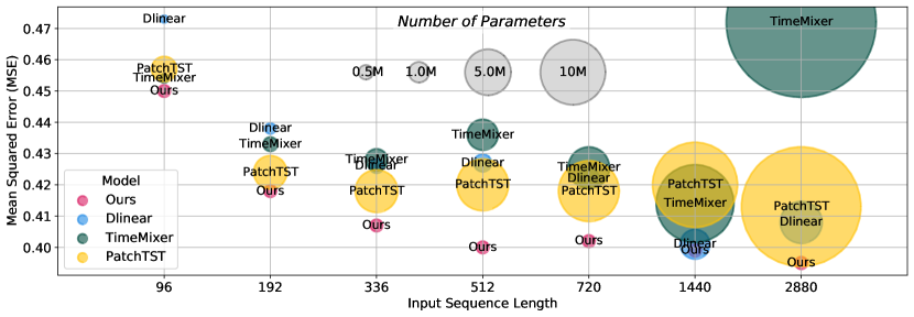
Figure 1: Experimental results illustrating the mean squared error (MSE) and the number of parameters with varying input sequence lengths on ETTm1. Each bubble represents a different model, with the bubble size indicating the number of parameters in millions—larger bubbles denote models with more parameters. Our model consistently shows the lowest MSE (i.e., best performance) with fewer parameters even for longer input sequences. The detailed results can be found in Table 3.

In this paper, we introduce a novel forecasting architecture named Cross-Attention-only Time Series transformer (CATS) that simplifies the original Transformer architecture by eliminating all self-attentions and focusing on the potential of cross-attentions. Specifically, our model establishes future horizon-dependent parameters as queries and treats past time series data as key and value pairs. This allows us to enhance parameter sharing and improve long-term forecasting performance. As shown in Figure 1, our model shows the lowest mean squared error (i.e., better forecasting performance) even for longer input sequences and with fewer parameters than existing models. Moreover, we demonstrate that this simplified architecture can provide a clearer understanding of how future predictions are derived from past data with individual attention maps for the specific forecasting horizon. Finally, through extensive experiments, we show that our proposed model not only achieves state-of-the-art performance but also requires fewer parameters and less memory consumption compared to previous Transformer models across various time series datasets.

2 Related Work

Time series transformers

Transformer models [19] have shown effective in various domains [5, 4, 15], with a novel encoder-decoder structure with self-attention, masked self-attention, and cross-attention. The self-attention mechanism is a key component for extracting semantic correlations between paired elements, even with identical input elements; however, autoregressive inference with self-attention requires quadratic time and memory complexity. Therefore, Informer [29] proposed directly predicting multi-steps, and a line of work, such as Autoformer [23], FEDformer [31], and Pyraformer [11], investigated the complexity issue in time series transformers. Simultaneously, unique properties of time series, such as stationarity [12], decomposition [23], frequency features [31], or cross-dimensional properties [28] were employed to modify the attention layer for forecasting tasks. Recently, researchers have investigated the essential architecture in transformers to capture long-term dependencies. PatchTST [14] became a de-facto standard Transformer model by patching the time series input in a channel-independence manner, which is widely used in following transformer forecasting models [13, 7]. On the other hand, Das et al. [3] emphasized the importance of decoder-only forecasting models, while they focused on zero-shot using pre-trained language models. However, none of them have investigated the importance of cross-attention for time series forecasting.

Temporal information encoding

Fixed temporal order in time series is the distinct property of time series, in contrast to the language domain where semantic information does not heavily depend on the word ordering [4]. Thus, some researchers have used learnable positional encoding in transformer models to embed time-dependent properties [9, 23]. However, Zeng et al. [26] first argued that self-attention is not suitable for time series due to its permutation invariant and anti-order properties. While they focus on building complex representations, they are inefficient in maintaining the original context of historical and future values. They rather proposed linear models without any embedding layer and demonstrated that it can achieve better performance than transformer models, particularly showing robust performance to long input sequences. Recent linear time series models outperformed previous transformer models with simple architectures by focusing on pre-processing and frequency-based properties [10, 2, 21]. On the other hand, Woo et al. [22] investigated the new line of works of time-index models, which try to model the underlying dynamics with given time stamps. These related works imply that preserving the order of time series sequences plays a crucial role in time series forecasting.

3 Proposed Methodology

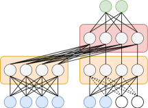
(a) Transformer

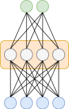
(b) Encoder

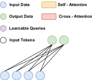
(c) Linear model

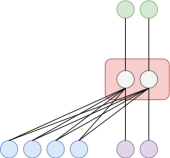
(d) Ours

Figure 2: Illustration of existing time series forecasting architectures and the proposed architecture.

3.1 Problem Definition and Notations

A multivariate time series forecasting task aims to predict future values $\bm{\tilde{X}}=\{{\mathbf{x}}_{L+1},\ldots,{\mathbf{x}}_{L+T}\}\in\mathbb{R}^{M\times T}$ with the prediction $\bm{\hat{X}}=\{\hat{{\mathbf{x}}}_{L+1},\ldots,\hat{{\mathbf{x}}}_{L+T}\}\in\mathbb{R}^{M\times T}$ based on past datasets $\bm{X}=\{{\mathbf{x}}_{1},\ldots,{\mathbf{x}}_{L}\}\in\mathbb{R}^{M\times L}$. Here, $T$ represents the forecasting horizon, $L$ denotes the input sequence length, and $M$ represents the dimension of time series data.

In traditional time series transformers, we feed the historical multivariate time series $\bm{X}$ to embedding layers, resulting in the historical embedding $\bm{H}_{L}\in\mathbb{R}^{D\times L}$. Here, $D$ is the embedding size. Note that, in channel-independence manners, the multivariate input is considered to separate univariate time series ${\mathbf{x}}\in\mathbb{R}^{1\times L}$. With patching [14], univariate time series ${\mathbf{x}}$ transforms into patches ${\mathbf{p}}=\texttt{Patch}({\mathbf{x}})\in\mathbb{R}^{P\times N_{L}}$ where $P$ is the size of each patch and $N_{L}$ is the number of input patches. Similar to non-patching situations, patches are fed to embedding layers $\bm{H}_{L}=\texttt{Embedding}({\mathbf{p}})\in\mathbb{R}^{D\times N_{L}}$.

Algorithm 1 Transformer Algorithm [19]

1:$\bm{Z}^{(\texttt{SA})}_{L}\,\,\leftarrow\texttt{LN}(\bm{H}_{L}+\texttt{SA}(\bm{H}_{L},\bm{H}_{L},\bm{H}_{L}))$

2:$\bm{Z}^{(\texttt{Enc})}_{L}\leftarrow\texttt{LN}(\bm{Z}^{(\texttt{SA})}_{L}+\texttt{MLP}(\bm{Z}^{(\texttt{SA})}_{L}))$

3:$\bm{Z}^{(\texttt{MSA})}_{T}\leftarrow\texttt{LN}(\bm{H}_{T}+\texttt{MSA}(\bm{H}_{T},\bm{H}_{T},\bm{H}_{T}))$

4:$\bm{Z}^{(\texttt{CA})}_{T}\,\,\leftarrow\texttt{LN}(\bm{Z}^{(\texttt{MSA})}_{T}+\texttt{CA}(\bm{Z}^{(\texttt{MSA})}_{T},\bm{Z}^{(\texttt{Enc})}_{L},\bm{Z}^{(\texttt{Enc})}_{L}))$

5:$\bm{Z}^{(\texttt{Dec})}_{T}\leftarrow\texttt{LN}(\bm{Z}^{(\texttt{CA})}_{T}+\texttt{MLP}(\bm{Z}^{(\texttt{CA})}_{T}))$

In Fig. 2, we illustrate the existing time series forecasting architectures and their key components. Transformer-based models, as shown in Fig. 2a, exhibit the most complex architecture. These models leverage Self-Attention (SA), Masked Self-Attention (MSA), and Cross-Attention (CA) to generate predictions. The detailed algorithm is formalized in Algorithm 1, where MLP represents the fully connected layer and LN represents LayerNorm. Note that, as input tokens $\bm{H}_{T}$ for cross-attention, positional embedding is often used [29, 23]. The output from the cross-attention, $\bm{Z}^{(\texttt{Dec})}_{T}\in\mathbb{R}^{D\times N_{T}}$, is subsequently used to produce the final prediction $\bm{\hat{X}}$ through additional layers. Particularly, if we remove the decoder structure from this transformer architecture as shown in Figure 2b, we call them encoder-only models [13, 14].

In contrast, as shown in Fig. 2c, simplified linear models, such as DLinear [26], remove all transformer-based components and rebuild direct linear connections between input and output data. By removing these transformer-based components, these models avoid temporal information loss problems [26] and the heavy computational load that increases quadratically with the input size $L$, i.e., $\mathcal{O}(L^{2})$. However, we emphasize that this temporal information loss and computational overhead, coupled with self-attention rather than the transformer architecture itself.

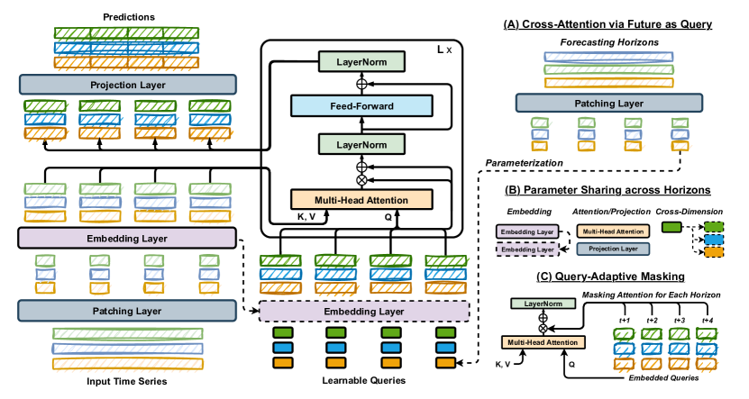
Figure 3: Illustration on the proposed model architecture. Our model removes all self-attentions from the original Transformer structure and focuses on cross-attentions. To fully utilize the cross-attention, we conceptualize the future horizon as queries and use the input time series (i.e., past time series) as keys and values (Fig. A). This simplified structure enables us to enhance the parameter sharing across forecasting horizons (Fig. B) and make use of query-adaptive masking (Fig. C) for performance.

3.2 Model Structure

We propose a model that not only preserves the temporal information of time series data similar to linear models but also utilizes the structural advantages of the transformer architecture. As illustrated in Figure 2d, cross-attention Transformer networks can maintain the periodic properties of time series, except for self-attention, which has permutation-invariant and anti-order characteristics. While Zeng et al. [26] replaced all attention layers with linear layers, we argue that this approach does not fully address the underlying issue; namely, the potential of the transformer architecture itself, excluding self-attention, has been overlooked. Therefore, we introduce a novel approach that prioritizes cross-attention without self-attention, leveraging advanced architectural designs of time series transformers, which linear models cannot utilize, such as patching [14].

Our proposed architecture consists of three key components: (A) Cross-Attention with Future as Query, (B) Parameter Sharing across Horizons, and (C) Query-Adaptive Masking. Fig. 3 illustrates how our model modifies the traditional transformer structure by removing self-attention and instead incorporating cross-attention, utilizing future data as the query. Additionally, we simplify the architecture by parameter sharing across forecasting horizons. We further enhance the performance through query-adaptive masking. The following paragraphs provide detailed descriptions of each component.

Cross-Attention via Future as Query

Similar to self-attention, the cross-attention mechanism employs three elements: key, query, and value. The distinctive feature of cross-attention is that the query originates from a different source than the key or value. Generally, the query component aims to identify the most relevant information among the keys and uses it to extract crucial data from the values [1, 27]. In the realm of time series forecasting, where predictions are often made for a specific target horizon—such as forecasting 10 steps ahead. Therefore, within this concept of forecasting, we argue that each future horizon should be regarded as a question, i.e., an independent query.

To implement this, we establish horizon-dependent parameters as learnable queries. As shown in Fig. 3, we begin by creating parameters for the specified forecasting horizon. For each of these virtualized parameters, we assign a fixed number of parameters to represent the corresponding horizon as learnable queries ${\mathbf{q}}$. For example, ${\mathbf{q}}_{i}$ is a horizon-dependent query at $L+i$. When patching is applied, these queries are then processed independently: each learnable query ${\mathbf{q}}\in\mathbb{R}^{P}$ is first fed into the embedding layer, and then fed into the multi-head attention with the embedded input time series patches as the key and value.

Based on these new query parameters, we can utilize a cross-attention-only structure in the decoder, resulting in an advantage in efficiency. In Table 1, we summarize the time complexity of recent transformer models and ours. The results indicate that our method only requires the time complexity of $\mathcal{O}({LT}/{P^{2}})$, where most of the transformer-based models require $\mathcal{O}({L}^{2})$ except FEDformer and Pyraformer. However, since these two models have an encoder-decoder and a relatively huge amount of parameters, they require 10x and 4x computational times than ours, respectively.

Table 1: Time complexity of transformer-based models to calculate attention outputs. Time refers to the inference time obtained by averaging 10 runs under $L=96$ and $T=720$ on Electricity.

Method	Encoder	Decoder	Time	Method	Encoder	Decoder	Time
Transformer [13]	$\mathcal{O}(L^{2})$	$\mathcal{O}(T(T+L))$	10.4ms	Informer [29]	$\mathcal{O}(L\log L)$	$\mathcal{O}(T(T+\log L))$	13.5ms
Autoformer [23]	$\mathcal{O}(L\log L)$	$\mathcal{O}\left(\left(L/2+H\right)\log\left(L/2+T\right)\right)$	24.1ms	Pyraformer [11]	$\mathcal{O}(L)$	$\mathcal{O}(T(T+L))$	11.2ms
FEDformer [31]	$\mathcal{O}(L)$	$\mathcal{O}\left(L/2+H\right)$	69.3ms	Crossformer [28]	$\mathcal{O}\left({M}L^{2}/{P^{2}}\right)$	$\mathcal{O}\left({M}T(T+L)/{P^{2}}\right)$	30.6ms
PatchTST [14]	$\mathcal{O}\left({L^{2}}/{P^{2}}\right)$	-	7.6ms	CATS (Ours)	-	$\mathcal{O}\left({LT}/{P^{2}}\right)$	7.0ms

Parameter Sharing across Horizons

One of the strongest benefits of cross-attention via future horizon as a query ${\mathbf{q}}$ is that each cross-attention is only calculated on the values from a single forecasting horizon and the input time series. Mathematically, for a prediction of future value $\hat{{\mathbf{x}}}_{L+i}$ can be expressed as a function solely dependent on the past samples $\bm{X}=[{\mathbf{x}}_{1},...,{\mathbf{x}}_{L}$] and ${\mathbf{q}}_{i}$, independent of ${\mathbf{q}}_{j}$ for all $i\neq j$ or $i$ and $j$ are not in the same patch.

This independent forecasting mechanism offers a notable advantage: a higher level of parameter sharing. As demonstrated in [14], significant reductions in the required number of parameters can be achieved in time series forecasting through parameter sharing between inputs or patches, enhancing computational efficiency. Regarding this, we propose parameter sharing across all possible layers — the embedding layer, multi-head attention, and projection layer — for every horizon-dependent query ${\mathbf{q}}$. In other words, all horizon queries ${\mathbf{q}}_{1},\dots,{\mathbf{q}}_{T}$ or ${\mathbf{q}}_{1},\dots,{\mathbf{q}}_{{N_{T}}}$ share the same embedding layer used for the input time series ${\mathbf{x}}_{1},\dots,{\mathbf{x}}_{L}$ or patches ${\mathbf{p}}_{1},\dots,{\mathbf{p}}_{N_{L}}$ before proceeding to the cross-attention layer, respectively. Furthermore, to maximize the parameter sharing, we also propose cross-dimension sharing that uses the same query parameters for all dimensions.

For the multi-head attention and projection layers, we apply the same algorithm across horizons. Notably, unlike the approach in PatchTST [14], we also share the projection layer for each prediction. Specifically, PatchTST employs a fully connected layer as the projection layer for the concatenated outputs $\bm{Z}^{(\texttt{Dec})}_{T}$. Thus, its number of parameters becomes $(D\times N_{L})\times T$. However, our model shares the same projection layer for each prediction. The number of parameters becomes $D\times P$, which is not proportionally increasing to $T$. This approach significantly reduces time complexity during both the training and inference phases. The details are presented in Appendix.

tableEffect of parameter sharing across horizons on the number of parameters for different forecasting horizons on ETTh1. Horizon w/ sharing w/o sharing 96 355,320 404,672 192 355,416 552,320 336 355,560 958,112 720 355,944 3,121,568

In Table 3.2, we outline the impact of parameter sharing across different forecasting horizons. In contrast to the model without parameter sharing, which exhibits a rapid increase in parameters as the forecasting horizon extends, our model, which shares all layers including the projection layer, maintains a nearly consistent number of parameters.

Additionally, all operations, including embedding and multi-head attention, are performed independently for each learnable query. This implies that the forecast for a specific horizon does not depend on other horizons. Such an approach allows us to generate distinct attention maps for each forecasting horizon, providing a clear understanding of how each prediction is derived. Please refer to Section 4.4.

Query-Adaptive Masking

Parameter sharing across horizons enhances the efficiency of our proposed architecture and simplifies the model. However, we observed that a high degree of parameter sharing could lead to overfitting to the keys and values (i.e., past time series data), rather than the queries (i.e., forecasting horizon). Specifically, the model may converge to generate similar or identical predictions, $\hat{{\mathbf{x}}}_{L+i}$ and $\hat{{\mathbf{x}}}_{L+j}$, despite receiving different horizon queries, ${\mathbf{q}}_{i}$ and ${\mathbf{q}}_{j}$ (i.e., the target horizons differ).

Therefore, to ensure the model focuses on each horizon-dependent query ${\mathbf{q}}$, we introduce a new technique that masks the attention outputs. As illustrated in the right-bottom figure of Fig. 3, for each horizon, we apply a mask to the direct connection from Multi-Head Attention to LayerNorm with a probability $p$. This mask prevents access to the input time series information, resulting in only the query to influence future value predictions. This selective disconnection, rather than the application of dropout in the residual connections, helps the layers to concentrate more effectively on the forecasting queries. We note that this approach can be related to stochastic depth in residual networks [8]. The stochastic depth technique has proven effective across various tasks, such as vision tasks [17, 25]. To the best of our knowledge, this is the first application of stochastic depth in Transformers for time series forecasting. A detailed analysis of query-adaptive masking can be found in Appendix.

In summary, the framework described in this section, including cross-attention via future as query, parameter sharing across horizons, and query-adaptive masking, is named the Cross-Attention-only Time Series transformer (CATS).

4 Experiments

In this section, we provide extensive experiments to provide the benefits of our proposed framework, CATS, including forecasting performance and computational efficiency. To this end, we use 7 different real-world datasets and 9 baseline models. For datasets, we use Electricity, ETT (ETTh1, ETTh2, ETTm1, and ETTm2), Weather, and Traffic. These datasets are provided in [23] for time series forecasting benchmark, detailed in Appendix.

For baselines, we utilize a wide range of various baselines, including the state-of-the-art long-term time series forecasting model TimeMixer [21], PatchTST [14], Timesnet [24], Crossformer [28], MICN [20], FiLM [30], DLinear [26], Autoformer [23], and Informer [29]. We used 4 NVIDIA RTX 4090 24GB GPUs with 2 Intel(R) Xeon(R) Gold 5218R CPUs @ 2.10GHz for all experiments.

4.1 Long-Term Time Series Forecasting Results

To ease comparison, we follow the settings of the most recent work [21] for long-term forecasting, which uses various horizon lengths with fixed 96 input sequence lengths. The detailed experimental settings can be found in Appendix. Table 2 summarizes the forecasting performance for all datasets and baselines. Our proposed model, CATS, demonstrates superior performance across multiple datasets in multivariate long-term forecasting tasks. Specifically, CATS consistently achieves the lowest Mean Squared Error (MSE) and Mean Absolute Error (MAE) on the Weather and Electricity datasets, with MSE values of 0.161 and 0.149 for the 96-step horizon, respectively, outperforming all other models. Additionally, for the Traffic dataset, CATS shows competitive performance, resulting in the second-best results with an MSE of 0.421 and MAE of 0.270 for the 96-step horizon. This indicates that CATS effectively captures the underlying patterns in diverse types of time series data. We observe consistent state-of-the-art performance of CATS in terms of error metrics, which highlights the high performance of our model in handling complex temporal dependencies. We also provide additional experiments with longer 512 input sequence lengths in Appendix.

Table 2: Multivariate long-term forecasting results with recent forecasting models and ours for unified hyperparameter settings. The best results are in bold and the second best are underlined.

Models		CATS		TimeMixer		PatchTST		Timesnet		Crossformer		MICN		FiLM		DLinear		Autoformer		Informer
Metric		MSE	MAE	MSE	MAE	MSE	MAE	MSE	MAE	MSE	MAE	MSE	MAE	MSE	MAE	MSE	MAE	MSE	MAE	MSE	MAE
Weather	96	0.161	0.207	0.163	0.209	0.186	0.227	0.172	0.220	0.195	0.271	0.198	0.261	0.195	0.236	0.195	0.252	0.266	0.336	0.300	0.384
	192	0.208	0.250	0.208	0.250	0.234	0.265	0.219	0.261	0.209	0.277	0.239	0.299	0.239	0.271	0.237	0.295	0.307	0.367	0.598	0.544
	336	0.264	0.290	0.251	0.287	0.284	0.301	0.246	0.337	0.273	0.332	0.285	0.336	0.289	0.306	0.282	0.331	0.359	0.395	0.578	0.523
	720	0.342	0.341	0.339	0.341	0.356	0.349	0.365	0.359	0.379	0.401	0.351	0.388	0.361	0.351	0.345	0.382	0.419	0.428	1.059	0.741
Electricity	96	0.149	0.237	0.153	0.247	0.190	0.296	0.168	0.272	0.219	0.314	0.180	0.293	0.198	0.274	0.210	0.302	0.201	0.317	0.274	0.368
	192	0.163	0.250	0.166	0.256	0.199	0.304	0.184	0.322	0.231	0.322	0.189	0.302	0.198	0.278	0.210	0.305	0.222	0.334	0.296	0.386
	336	0.180	0.268	0.185	0.277	0.217	0.319	0.198	0.300	0.246	0.337	0.198	0.312	0.217	0.300	0.223	0.319	0.231	0.443	0.300	0.394
	720	0.219	0.302	0.225	0.310	0.258	0.352	0.220	0.320	0.280	0.363	0.217	0.330	0.278	0.356	0.258	0.350	0.254	0.361	0.373	0.439
Traffic	96	0.421	0.270	0.462	0.285	0.526	0.347	0.593	0.321	0.644	0.429	0.577	0.350	0.647	0.384	0.650	0.396	0.613	0.388	0.719	0.391
	192	0.436	0.275	0.473	0.296	0.522	0.332	0.617	0.336	0.665	0.431	0.589	0.356	0.600	0.361	0.598	0.370	0.616	0.382	0.696	0.379
	336	0.453	0.284	0.498	0.296	0.517	0.334	0.629	0.336	0.674	0.420	0.594	0.358	0.610	0.367	0.605	0.373	0.622	0.337	0.777	0.420
	720	0.484	0.303	0.506	0.313	0.552	0.352	0.640	0.350	0.683	0.424	0.613	0.361	0.691	0.425	0.645	0.394	0.660	0.408	0.864	0.472
ETTm1	96	0.318	0.357	0.320	0.357	0.352	0.374	0.338	0.375	0.404	0.426	0.365	0.387	0.353	0.370	0.346	0.374	0.505	0.475	0.672	0.571
	192	0.357	0.377	0.361	0.381	0.390	0.393	0.374	0.387	0.450	0.451	0.403	0.408	0.389	0.387	0.382	0.391	0.553	0.496	0.795	0.669
	336	0.387	0.401	0.390	0.404	0.421	0.414	0.410	0.411	0.532	0.515	0.436	0.431	0.421	0.408	0.415	0.415	0.621	0.537	1.212	0.871
	720	0.448	0.437	0.454	0.441	0.462	0.449	0.478	0.450	0.666	0.589	0.489	0.462	0.481	0.441	0.473	0.451	0.671	0.561	1.166	0.823
ETTm2	96	0.178	0.261	0.175	0.258	0.183	0.270	0.187	0.267	0.287	0.366	0.197	0.296	0.183	0.266	0.193	0.293	0.255	0.339	0.365	0.453
	192	0.248	0.308	0.237	0.299	0.255	0.314	0.249	0.309	0.414	0.492	0.284	0.361	0.248	0.305	0.284	0.361	0.281	0.340	0.533	0.563
	336	0.304	0.343	0.298	0.340	0.309	0.347	0.321	0.351	0.597	0.542	0.381	0.429	0.309	0.343	0.382	0.429	0.339	0.372	1.363	0.887
	720	0.402	0.402	0.391	0.396	0.412	0.404	0.408	0.403	1.730	1.042	0.549	0.522	0.410	0.400	0.558	0.525	0.433	0.432	3.379	1.338
ETTh1	96	0.371	0.395	0.375	0.400	0.460	0.447	0.384	0.402	0.423	0.448	0.426	0.446	0.438	0.433	0.397	0.412	0.449	0.459	0.865	0.713
	192	0.426	0.422	0.429	0.421	0.512	0.477	0.436	0.429	0.471	0.474	0.454	0.464	0.493	0.466	0.446	0.441	0.500	0.482	1.008	0.792
	336	0.437	0.432	0.484	0.458	0.546	0.496	0.638	0.469	0.570	0.546	0.493	0.487	0.547	0.495	0.489	0.467	0.521	0.496	1.107	0.809
	720	0.474	0.461	0.498	0.482	0.544	0.517	0.521	0.500	0.653	0.621	0.526	0.526	0.586	0.538	0.513	0.510	0.514	0.512	1.181	0.865
ETTh2	96	0.287	0.341	0.289	0.341	0.308	0.355	0.340	0.374	0.745	0.584	0.372	0.424	0.322	0.364	0.340	0.394	0.346	0.388	3.755	1.525
	192	0.361	0.388	0.372	0.392	0.393	0.405	0.402	0.414	0.877	0.656	0.492	0.492	0.404	0.414	0.482	0.479	0.456	0.453	5.602	1.931
	336	0.374	0.403	0.386	0.414	0.427	0.436	0.452	0.452	1.043	0.731	0.607	0.555	0.435	0.445	0.591	0.541	0.482	0.486	4.721	1.835
	720	0.412	0.433	0.412	0.434	0.436	0.450	0.462	0.468	1.104	0.763	0.824	0.655	0.447	0.458	0.839	0.661	0.515	0.511	3.647	1.625

4.2 Efficient and Robust Forecasting for Long Input Sequences

Zeng et al. [26] observed that many models experience a decline in performance when using long input sequences for time series forecasting. To address this, some approaches have been developed to capture long-term dependencies. For instance, TimeMixer [21] employs linear models with mixed scale, and PatchTST [14] utilizes an encoder network to encode long-term information. However, these models still have computational issues, particularly in terms of escalating memory and parameter requirements. Thus, in this subsection, we provide a comparison between previous models and ours in terms of efficient and robust forecasting for long input sequences.

First of all, to provide a fair comparison, we summarize the number of parameters, GPU memory consumption, and forecasting performance of comparison models with varying input lengths. As summarized in Table 3, existing complex models, such as PatchTST and TimeMixer, suffer from increased parameters and computational burdens when performing forecasting with long input lengths. Although DLinear uses fewer parameters and less GPU memory, its performance is limited due to its linear structure in capturing non-linearity patterns. Considering both performance and efficiency, the proposed model demonstrates robust performance improvement even with longer input lengths. In Appendix, we provide additional experimental results supporting these findings.

Table 3: Comparison of models with the number of parameters, GPU memory consumption, and MSE across different input sequence lengths on ETTm1. Full results with more diverse input lengths are presented in Appendix.

	Parameters				GPU Memory				MSE
Input Length	336	720	1440	2880	336	720	1440	2880	336	720	1440	2880
PatchTST	4.3M	8.7M (2.0x)	17.0M (4.0x)	33.6M (7.9x)	3.5GB	7.4GB (2.1x)	22.0GB (6.3x)	58.6GB (16.9x)	0.418	0.418	0.420	0.412
TimeMixer	1.1M	4.1M (3.6x)	14.2M (12.6x)	52.9M (46.8x)	2.9GB	3.9GB (1.3x)	5.9GB (2.0x)	10.3GB (3.6x)	0.428	0.425	0.414	0.472
DLinear	0.5M	1.0M (2.1x)	2.1M (4.2x)	4.2M (8.5x)	1.1GB	1.1GB (1.0x)	1.2GB (1.0x)	1.2GB (1.1x)	0.426	0.422	0.401	0.408
CATS	0.4M	0.4M (1.0x)	0.4M (1.0x)	0.4M (1.1x)	1.9GB	2.1GB (1.1x)	2.7GB (1.4x)	3.8GB (2.0x)	0.407	0.402	0.399	0.395

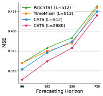
(a) Model Performance

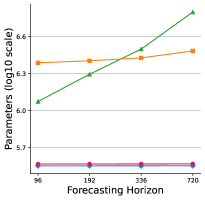
(b) Parameter Efficiency

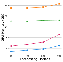
(c) Memory Efficiency

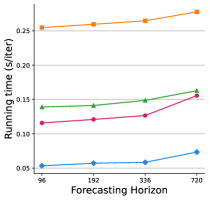
(d) Running Time Efficiency

Figure 4: Efficiency and performance analysis for time series forecasting models. We summarize the forecasting performance, number of parameters, GPU memory consumption, and running time with varying forecasting horizon lengths on Traffic. The running time is averaged from 300 iterations.

Furthermore, we conduct a deeper comparison between transformer-based models. Especially, TimeMixer [21] argues that their model outperforms PatchTST [14] in the setting of long input sequences. Regarding this setting, we also conduct an experiment on $L=512$. We summarize the results in Fig. 4. Among these transformer-based models, our model achieves the lowest MSE for most forecasting horizons. Moreover, our model requires even a lower number of parameters, GPU memory, and running time. Especially, for parameter efficiency, CATS shows significant differences even on a log scale due to its efficient parameter-sharing. Fig. 4c highlights GPU memory usage across different forecasting horizons. While PatchTST and TimeMixer consume significantly more memory, CATS maintains a low and stable memory consumption, demonstrating superior memory efficiency. In Fig. 4d CATS also consistently achieves lower running times compared to PatchTST and TimeMixer.

Additionally, we also compare the same factors when we use a longer input length $L=2880$. As more input length is used, the forecasting performance of our model outperforms all other models. Most importantly, while the computational complexity increases as input length increases, our model achieves a faster running time, compared to other models with a 512 input sequence length. Overall, these results emphasize the efficiency and performance advantages of our model, particularly in terms of parameter count, memory usage, and running time.

4.3 Replacement of Cross-attention with Self-attention

In our propose structure, we mainly use cross-attention rather than self-attention due to the forecasting-unfriendly properties of self-attention. To verify the effectiveness of cross-attention in the proposed structure, we replace the cross-attention layers with self-attention layers while maintaining other structures. In Table 4, we gradually replace the cross-attention with self-attention (SA) among a total of three cross-attention layers. To maintain the original transformer structure, we set the maximum replacement as two. As shown in this table, we confirm the effectiveness of the cross-attention mechanism compared to using self-attention layers. Specifically, the zero SA, which is our model, shows better performance than using SA for almost all cases except only one case.

Table 4: Performance comparison on models with three attention layers. We replace one or more cross-attentions (CA) with self-attentions (SA) in our model. In total, there are three cross-attentions in all settngs and ‘Zero SA’ stands for our model. The best results are in bold.

Dataset	Electricity						ETTm1
Case	Zero SA		One SA		Two SA		Zero SA		One SA		Two SA
Metric	MSE	MAE	MSE	MAE	MSE	MAE	MSE	MAE	MSE	MAE	MSE	MAE
96	0.126	0.218	0.128	0.220	0.133	0.225	0.283	0.340	0.284	0.338	0.284	0.340
192	0.144	0.235	0.150	0.238	0.153	0.245	0.319	0.363	0.331	0.373	0.324	0.368
336	0.159	0.252	0.167	0.257	0.169	0.263	0.351	0.385	0.376	0.401	0.369	0.400
720	0.194	0.283	0.205	0.293	0.210	0.300	0.400	0.414	0.429	0.437	0.442	0.445

4.4 Understanding Periodic Patterns with Cross-Attention

As noted in Section 3.2, in our proposed model, all operations including embedding and multi-head attention are performed independently for each learnable query. In other words, the forecast for a specific horizon does not depend on other horizons. This approach allows us to gain a clear understanding of how each prediction is calculated. Therefore, in this subsection, we visualize how the proposed model understands the periodic properties.

To provide an easy understanding, we here consider a simple time series forecasting task with data that consists of two independent signals as follows:

$${\mathbf{x}}(t) =\{x_{(t\bmod\tau)}\}^{\infty}_{t=1},\quad x_{i}\sim\mathcal{N}(0,1)\quad(i=0,1,\ldots,\tau-1),$$ (1)

$${\bm{y}}(t) =\begin{cases}+k&\text{if }t\equiv 0\quad\pmod{S}\\ -k&\text{if }t\equiv\frac{1}{2}S\text{ }\pmod{S}.\end{cases}$$ (2)

For prediction, we use an input sequence length $L=48$ and a forecasting horizon $T=72$ with signals ${\mathbf{x}}(t)$ and ${\bm{y}}(t)$ are defined with $\tau=24$, $S=8$, and $k=5$. The patch length is set to 4 without overlapping to elucidate the distinct periodic components with 2 attention heads.

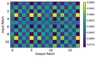
(a) Cross-attention score map of head 1

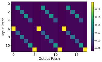
(b) Cross-attention score map of head 2

Figure 5: Score map of cross-attentions between input and output patches.

In Fig. 5, we illustrate a score map (12$\times$18) of the cross-attention from the trained CATS. Since both patch length and stride are set to 4, each patch will contain exactly one shock value. We observe that the cross-attentions capture the shocks within the signal and the periodicity of the signal in Fig. 5a and Fig. 5b, respectively. Fig. 5a shows that patches an even number of steps before the current patch contain the shocks of the same direction, resulting in higher attention scores, while odd-numbered steps have lower scores. Moreover, the correlation over 24 steps is clearly demonstrated in patches spaced by multiples of 6 steps, as shown in Fig. 5b. This periodic pattern ensures that the attention mechanism effectively captures the periodicity in ${\mathbf{x}}(t)$, reflecting the model’s ability to leverage this periodic information for more accurate predictions. In Appendix, we provide a detailed explanation.

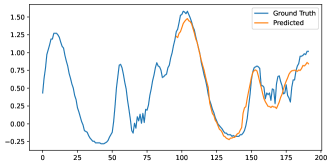
(a) Forecasting results

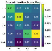
(b) Averaged score

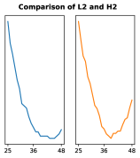
(c) L2-H2

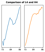
(d) L4-H4

Figure 6: Illustration of (a) forecasting result, (b) averaged cross-attention score, and (c,d) patches with the highest score on ETTm1. The score map is averaged from all the heads across layers.

Fig. 6 illustrates (a) forecasting results, (b) a cross-attention score map (5$\times$4) on the ETTm1 dataset, and (c, d) the two pairs with the highest attention scores. We predict 96 steps with input sequence length 96 on ETTm1. The input patches consist of four patches of 24 lengths and one padding patch. As shown in Fig. 6c and 6d, the patches with high attention scores exhibit similar temporal patterns, demonstrating the ability of CATS to detect sequential and periodic patterns.

5 Conclusion

Based on our study, we exploit the advantages of Transformer models in time series forecasting by removing self-attentions and developing a new cross-attention-based architecture. We believe that our model establishes a strong baseline for such forecasting tasks and offers further insights into the complexities of long-term forecasting problems. Our findings provide a reevaluation of self-attentions in this domain, and we hope that future research can critically assess the efficacy and efficiency across various time series analysis tasks. As a limitation, our proposed methods assume channel independence between variables based on the recent work [14]. As the time series data in the real-world are highly correlated, we hope future research can address cross-variate dependency with reduced computation complexity based on the proposed architecture.

Appendix A Experimental settings

A.1 Datasets

We evaluated the performance using seven datasets commonly used in long-term time series forecasting, including Weather, Traffic, Electricity, and ETT (ETTh1, ETTh2, ETTm1, and ETTm2). These datasets capture a range of periodic characteristics and scenarios that are difficult to predict in the real world, making them highly suitable for tasks, such as long-term time series forecasting, generation, and imputation. Details of these datasets are described in Table 5. These datasets are provided in Wu et al. [23].

Table 5: Details of 7 real-world datasets.

	Dimension	Frequency	Timesteps	Information
Weather	21	10-min	52,696	Weather
Electricity	321	Hourly	17,544	Electricity
Traffic	862	Hourly	26,304	Transportation
ETTh1	7	Hourly	17,420	Temperature
ETTh2	7	Hourly	17,420	Temperature
ETTm1	7	15-min	69,680	Temperature
ETTm2	7	15-min	69,680	Temperature

A.2 Hyperparameter Settings

In every experiment in our paper, following [14], we fixed the random seed of 2021 to enhance the reproducibility of our experiments. Additionally, following numerous studies in the field of time series forecasting [14], we fixed the input sequence length $L=96$. For the forecasting horizon $T$, we also used the widely accepted values, i.e., $[96,192,336,720]$. For our model, in all configurations, we adopt the GeGLU activation function [16] between the two linear layers in the feed-forward network for our model. Additionally, we use learnable positional embedding parameters for the input data and omit positional embeddings for learnable queries to avoid redundant parameter learning. For Table 2, our model uses three cross-attention layers with embedding size $D=256$, number of attention heads $H=32$. Specifically, to avoid overfitting on small datasets [14], we use patch length 48 on the ETTh1 and ETTh2 datasets. Table 6 shows further details of hyperparameter settings.

Table 6: Experimental settings mainly used for the main paper.

Metric	Layers	Embedding Size	Query Sharing	Input Sequence Length	Batch Size	Epoch	Learning Rate
Weather	3	256	False	96	64	30	$10^{-3}$
Electricity	3	256	False	96	32	30	$10^{-3}$
Traffic	3	256	True	96	32	100	$10^{-3}$
ETTh1	3	256	False	96	256	10	$10^{-3}$
ETTh2	3	256	True	96	256	10	$10^{-3}$
ETTm1	3	256	False	96	128	30	$10^{-3}$
ETTm2	3	256	True	96	128	30	$10^{-3}$

Appendix B Additional Experimental Results

B.1 Performance with Longer Input Sequences

In Table 3, we compared models with the number of parameters, GPU memory consumption, and MSE across different input lengths on ETTm1 with varying input sequence lengths. In this section, we provide comprehensive results on longer input sequence lengths $L=512$. The detailed parameters can be found in Table 7 and the corresponding experimental results are summarized in Table 8. As with unified hyperparameter settings, we follow the settings of the most recent work [21] to ease comparison. Overall, the experimental results clearly illustrate the superiority of CATS over recent forecasting models across multiple datasets and prediction horizons. CATS consistently shows the lowest Mean Squared Error (MSE) and Mean Absolute Error (MAE) across a variety of datasets and forecast horizons. For instance, on Electricity, at the 96 forecast horizon, CATS achieves the best MSE score of 0.144 and the best MAE score of 0.189, underscoring its accuracy in predicting electrical demand.

Table 7: Experimental settings with an input sequence length of 512.

Metric	Layers	Embedding Size	Query Sharing	Input Sequence Length	Batch Size	Epoch	Learning Rate
Weather	3	128	False	512	128	30	$10^{-3}$
Electricity	3	128	False	512	32	30	$10^{-3}$
Traffic	3	128	True	512	32	100	$10^{-3}$
ETTh1	3	256	False	512	128	10	$10^{-3}$
ETTh2	3	256	True	512	256	10	$10^{-3}$
ETTm1	3	128	False	512	128	30	$10^{-3}$
ETTm2	3	256	True	512	128	30	$10^{-3}$

Table 8: Multivariate long-term forecasting results with an input sequence length of 512. The best results are in bold and the second best are underlined.

Models		CATS		TimeMixer		PatchTST		Timesnet		Crossformer		MICN		FiLM		DLinear		Autoformer		Informer
Metric		MSE	MAE	MSE	MAE	MSE	MAE	MSE	MAE	MSE	MAE	MSE	MAE	MSE	MAE	MSE	MAE	MSE	MAE	MSE	MAE
Weather	96	0.144	0.199	0.147	0.197	0.149	0.198	0.172	0.220	0.232	0.302	0.161	0.229	0.199	0.262	0.176	0.237	0.266	0.336	0.300	0.384
	192	0.188	0.240	0.189	0.239	0.194	0.241	0.219	0.261	0.371	0.410	0.220	0.281	0.228	0.288	0.220	0.282	0.307	0.367	0.598	0.544
	336	0.238	0.280	0.241	0.280	0.306	0.282	0.246	0.337	0.495	0.515	0.278	0.331	0.267	0.323	0.265	0.319	0.359	0.395	0.578	0.523
	720	0.308	0.329	0.310	0.330	0.314	0.334	0.365	0.359	0.526	0.542	0.311	0.356	0.319	0.361	0.323	0.362	0.419	0.428	0.590	0.741
Electricity	96	0.126	0.218	0.129	0.224	0.129	0.222	0.168	0.272	0.150	0.251	0.164	0.269	0.154	0.267	0.140	0.237	0.201	0.317	0.274	0.368
	192	0.144	0.235	0.140	0.220	0.147	0.240	0.184	0.322	0.161	0.260	0.177	0.285	0.164	0.258	0.153	0.249	0.222	0.334	0.296	0.386
	336	0.159	0.252	0.161	0.255	0.163	0.259	0.198	0.300	0.182	0.281	0.193	0.304	0.188	0.283	0.169	0.267	0.231	0.338	0.300	0.394
	720	0.194	0.283	0.194	0.287	0.197	0.290	0.220	0.320	0.251	0.339	0.212	0.321	0.236	0.332	0.203	0.301	0.254	0.361	0.373	0.439
Traffic	96	0.352	0.243	0.360	0.249	0.360	0.249	0.593	0.321	0.514	0.267	0.519	0.309	0.416	0.294	0.410	0.282	0.613	0.388	0.719	0.391
	192	0.373	0.253	0.375	0.250	0.379	0.256	0.617	0.336	0.549	0.252	0.537	0.315	0.408	0.288	0.423	0.287	0.616	0.382	0.696	0.379
	336	0.387	0.260	0.385	0.270	0.392	0.264	0.629	0.336	0.530	0.300	0.534	0.313	0.425	0.298	0.436	0.296	0.622	0.337	0.777	0.420
	720	0.425	0.281	0.430	0.281	0.432	0.286	0.640	0.350	0.573	0.313	0.577	0.325	0.520	0.353	0.466	0.315	0.660	0.408	0.864	0.472
ETTh1	96	0.373	0.401	0.361	0.390	0.370	0.400	0.384	0.402	0.418	0.438	0.421	0.431	0.422	0.432	0.375	0.399	0.449	0.459	0.865	0.713
	192	0.401	0.421	0.409	0.414	0.413	0.429	0.436	0.429	0.539	0.517	0.474	0.487	0.462	0.458	0.405	0.416	0.500	0.482	0.080	0.792
	336	0.415	0.434	0.430	0.429	0.422	0.440	0.638	0.469	0.709	0.638	0.569	0.551	0.501	0.483	0.439	0.443	0.521	0.496	0.107	0.809
	720	0.435	0.446	0.445	0.460	0.447	0.468	0.521	0.500	0.733	0.636	0.770	0.672	0.544	0.526	0.472	0.490	0.514	0.512	0.181	0.865
ETTh2	96	0.256	0.328	0.271	0.330	0.274	0.337	0.340	0.374	0.425	0.463	0.299	0.364	0.323	0.370	0.289	0.353	0.358	0.397	0.755	0.525
	192	0.311	0.366	0.317	0.402	0.314	0.382	0.231	0.322	0.473	0.500	0.441	0.454	0.391	0.415	0.383	0.418	0.456	0.453	0.602	0.931
	336	0.319	0.382	0.332	0.396	0.329	0.384	0.452	0.452	0.581	0.562	0.654	0.567	0.415	0.440	0.448	0.465	0.482	0.486	0.721	0.835
	720	0.395	0.438	0.342	0.408	0.379	0.422	0.462	0.468	0.775	0.665	0.956	0.716	0.441	0.459	0.605	0.551	0.515	0.511	0.647	0.625
ETTm1	96	0.283	0.340	0.291	0.340	0.293	0.346	0.338	0.375	0.361	0.403	0.316	0.362	0.302	0.345	0.299	0.343	0.505	0.475	0.672	0.571
	192	0.319	0.363	0.327	0.365	0.333	0.370	0.374	0.387	0.387	0.422	0.363	0.390	0.338	0.368	0.335	0.365	0.553	0.496	0.795	0.669
	336	0.351	0.385	0.360	0.381	0.369	0.392	0.410	0.411	0.605	0.572	0.408	0.426	0.373	0.388	0.369	0.386	0.621	0.537	0.212	0.871
	720	0.400	0.414	0.415	0.417	0.416	0.420	0.478	0.450	0.703	0.645	0.481	0.476	0.420	0.420	0.425	0.421	0.671	0.561	0.166	0.823
ETTm2	96	0.165	0.256	0.164	0.254	0.166	0.256	0.187	0.267	0.275	0.358	0.179	0.275	0.165	0.256	0.167	0.260	0.255	0.339	0.365	0.453
	192	0.221	0.297	0.223	0.295	0.223	0.296	0.249	0.309	0.345	0.400	0.307	0.376	0.222	0.296	0.224	0.303	0.281	0.340	0.533	0.563
	336	0.274	0.334	0.279	0.330	0.274	0.329	0.321	0.351	0.657	0.528	0.325	0.388	0.277	0.333	0.281	0.342	0.339	0.372	0.363	0.887
	720	0.362	0.390	0.359	0.383	0.362	0.385	0.408	0.403	0.208	0.753	0.502	0.490	0.371	0.389	0.397	0.421	0.422	0.419	0.379	0.388

B.2 Additional Results for Section 4.2

Table 9: Comparison of models with the number of parameters, GPU memory consumption, and MSE across different input sequence lengths on ETTm1. Full results of Table 3.

	Parameters across different input lengths
Models	96	192	336	512	720	1440	2880
PatchTST	1,506,384	2,612,304	4,271,184	6,298,704	8,694,864	16,989,264	33,578,064
TimeMixer	190,313	484,217	1,129,193	2,250,137	4,046,633	14,211,593	52,912,313
DLinear	139,680	277,920	485,280	738,720	1,038,240	2,075,040	4,148,640
CATS	360,264	360,776	361,544	362,440	363,592	367,432	375,112
	GPU Memory Consumption across different input lengths
Models	96	192	336	512	720	1440	2880
PatchTST	2,234MB	2,650MB	3,484MB	4,914MB	7,368MB	2,1968MB	58,590MB
TimeMixer	2,204MB	2,522MB	2,914MB	3,414MB	3,888MB	5,876MB	10,324MB
DLinear	1,098MB	1,102MB	1,104MB	1,114MB	1,114MB	1,154MB	1,214MB
CATS	1,712MB	1,796MB	1,884MB	2,042MB	2,140MB	2,700MB	3,826MB
	MSE across different input lengths
Models	96	192	336	512	720	1440	2880
PatchTST	0.457	0.424	0.418	0.420	0.418	0.420	0.413
TimeMixer	0.454	0.433	0.428	0.436	0.425	0.414	0.472
DLinear	0.473	0.438	0.426	0.427	0.422	0.401	0.408
CATS	0.450	0.418	0.407	0.400	0.402	0.399	0.395

Table 10: Comparison of models with the number of parameters, GPU memory consumption, and MSE across different input sequence lengths on Weather.

	Parameters across different input lengths
Models	96	192	336	512	720	1440	2880
PatchTST	1,506,384	2,612,304	4,271,184	6,298,704	8,694,864	16,989,264	33,578,064
TimeMixer	219,249	595,305	1,465,569	3,028,185	5,582,529	20,343,969	77,423,049
DLinear	139,680	277,920	485,280	738,720	1,038,240	2,075,040	4,148,640
CATS	370,344	370,856	371,624	372,520	373,672	377,512	385,192
	GPU Memory Consumption across different input lengths
Models	96	192	336	512	720	1440	2880
PatchTST	1,680MB	2,110MB	2,762MB	4,596MB	5,726MB	16,472MB	45,278MB
TimeMixer	1,894MB	2,154MB	2,728MB	3,414MB	4,356MB	8,358MB	20,624MB
DLinear	1,106MB	1,114MB	1,188MB	1,188MB	1,188MB	1,362MB	1,632MB
CATS	1,522MB	1,590MB	1,665MB	1,755MB	1,892MB	2,282MB	3,140MB
	MSE across different input lengths
Models	96	192	336	512	720	1440	2880
PatchTST	0.351	0.336	0.320	0.315	0.309	0.308	0.312
TimeMixer	0.339	0.331	0.318	0.319	0.324	0.318	0.327
DLinear	0.346	0.334	0.325	0.320	0.316	0.311	0.309
CATS	0.342	0.325	0.314	0.308	0.305	0.301	0.291

We provide additional experimental results to support the findings discussed in Section 4.2. Tables 9 and 10 summarize detailed comparisons of the number of parameters, GPU memory consumption, and MSE across different input lengths for the ETTm1 and Weather datasets, respectively. The linear models, TimeMixer and DLinear, exhibit smaller parameters for shorter input lengths. Despite CATS having slightly more parameters than TimeMixer for smaller inputs, it outperforms in terms of memory usage and MSE. This suggests that CATS is more efficient and effective in handling shorter inputs. For PatchTST, the number of parameters does not increase within the actual Transformer backbone as the input length increases. However, due to the need to flatten and project all inputs at the end, the parameters scale linearly with the input length. This highlights a limitation of the Encoder’s architecture. On the other hand, TimeMixer’s parameters grow almost quadratically as the input length doubles. Similarly, DLinear’s parameters increase linearly with the input length. Our proposed model, CATS demonstrates significant efficiency through parameter sharing, where the parameters hardly increase with longer inputs. Notably, from an input length of 336, CATS has fewer parameters than DLinear, showcasing the deep learning model’s advantage in detecting inherent patterns in the data.

Regarding GPU memory consumption, we observe that both PatchTST and TimeMixer require significantly more GPU memory as the input length increases. For example, PatchTST’s GPU memory usage scales drastically, making it less feasible for long input sequences. TimeMixer also shows an increase in GPU memory consumption, although it is less severe than PatchTST. In contrast, DLinear maintains a relatively constant GPU memory usage, demonstrating its efficiency in terms of computational resources. However, CATS stands out by offering a balanced approach, with moderate GPU memory usage that scales more favorably compared to PatchTST and TimeMixer. This balance between memory efficiency and performance is crucial for practical applications requiring long-term time series forecasting.

Furthermore, when analyzing the MSE across different input lengths, CATS consistently shows the best performance. It maintains lower MSE compared to other models across all input lengths. This robustness in performance, combined with its efficient parameter and memory usage, highlights the superiority of CATS in long-term time series forecasting tasks. Overall, these results show the advantages of CATS in terms of parameter efficiency, GPU memory consumption, and forecasting accuracy. These findings support the proposed model’s potential for practical and scalable time series forecasting solutions.

Table 11 presents the full results on the Traffic dataset. Here, we use the Traffic dataset with a batch size of 8. All GPU memory consumption was measured in a setting using four multi-GPUs. As shown in Table 11, CATS with a 2880 input sequence length consistently outperforms models with a 512 input sequence length, including PatchTST and TimeMixer. Specifically, CATS demonstrates fewer parameters, lower GPU memory consumption, and faster running speeds. These results highlight the efficiency of CATS with large input sizes. The Traffic dataset, characterized by high-dimensional data, shows a significant reduction in MSE when using longer input sequences.

Table 12 provides the full results on the Electricity dataset. Similar to the Traffic dataset, CATS shows superior efficiency in training, particularly with an input size of 2880, across all cases. Here, we use the Electricity dataset with a batch size of 32. All GPU memory consumption was measured in a setting using four multi-GPUs. In this experiment, CATS with a 512 input sequence length did not use parameter sharing for queries, while CATS with a 2880 input sequence length did. This demonstrates the effectiveness of query parameter sharing when utilizing large amounts of data for training. The results confirm that query sharing among dimensions leads to greater efficiency and improved performance.

Table 11: Comparison of models with the number of parameters, GPU memory consumption, running speed, and MSE across different forecasting horizon sizes on Traffic. Full results of Fig. 4.

Horizon	Models	Paramters	Gpu Memory	Running Time	MSE
96	PatchTST	1,186,272	28.54GB	0.1390s/iter	0.360
	TimeMixer	2,442,961	38.12GB	0.2548s/iter	0.360
	CATS ($L=512$)	357,496	5.81GB	0.0533s/iter	0.352
	CATS ($L=2880$)	370,168	9.79GB	0.1158s/iter	0.339
192	PatchTST	1,972,800	28.34GB	0.1412s/iter	0.379
	TimeMixer	2,535,505	38.13GB	0.2596s/iter	0.375
	CATS ($L=512$)	357,592	6.73GB	0.0571s/iter	0.373
	CATS ($L=2880$)	370,264	11.10GB	0.1209s/iter	0.362
336	PatchTST	3,152,592	28.91GB	0.1487s/iter	0.392
	TimeMixer	2,674,321	38.69GB	0.2647s/iter	0.385
	CATS ($L=512$)	357,736	7.46GB	0.0584s/iter	0.387
	CATS ($L=2880$)	370,408	12.72GB	0.1266s/iter	0.379
720	PatchTST	6,298,704	29.15GB	0.1628s/iter	0.432
	TimeMixer	3,044,497	41.17GB	0.2777s/iter	0.430
	CATS ($L=512$)	358,120	10.10GB	0.0734s/iter	0.423
	CATS ($L=2880$)	370,792	18.40GB	0.1556s/iter	0.420

Table 12: Comparison of models with the number of parameters, GPU memory consumption, running speed, and MSE across different forecasting horizon sizes on Electricity.

Horizon	Models	Paramters	Gpu Memory	Running Time	MSE
96	PatchTST	1,186,272	40.36GB	0.2021s/iter	0.129
	TimeMixer	2,429,049	33.80GB	0.2118s/iter	0.129
	CATS ($L=512$)	388,216	6.89GB	0.0587s/iter	0.126
	CATS ($L=2880$)	370,168	12.82GB	0.1653s/iter	0.126
192	PatchTST	1,972,800	40.39GB	0.2048s/iter	0.147
	TimeMixer	2,521,593	33.81GB	0.2212s/iter	0.140
	CATS ($L=512$)	419,032	8.07GB	0.0636s/iter	0.144
	CATS ($L=2880$)	370,264	14.70GB	0.1725s/iter	0.139
336	PatchTST	3,152,592	40.42GB	0.2070s/iter	0.163
	TimeMixer	2,660,409	34.24GB	0.2314s/iter	0.161
	CATS ($L=512$)	465,256	9.15GB	0.0690s/iter	0.159
	CATS ($L=2880$)	370,408	17.38GB	0.1839s/iter	0.153
720	PatchTST	6,298,704	41.40GB	0.2313s/iter	0.197
	TimeMixer	3,030,585	36.13GB	0.2478s/iter	0.194
	CATS ($L=512$)	588,520	12.77GB	0.0964s/iter	0.194
	CATS ($L=2880$)	370,792	25.86GB	0.2262s/iter	0.183

B.3 Ablation Study on Query-adaptive Masking

In this section, we demonstrate the effectiveness of query-adaptive masking compared to dropout, which is a widely adopted technique in transformer-based forecasting models. We consider four different setups: using only dropout, using query-adaptive masking with fixed probabilities, query-adaptive masking with linearly increasing probabilities, and using both methods simultaneously. As shown in Fig. 7, the query-adaptive masking shows better forecasting performance and faster converge speed compared to dropout. Applying a gradually increasing masking probability based on the horizon predicted by the query shows slight performance improvements over using a fixed probability or combining with dropout. In contrast, using dropout alone shows noticeable differences in both convergence speed and overall performance. This demonstrates that when multiple inputs with different forecasting horizons share a single model, probabilistic masking is more beneficial for model training than dropout.

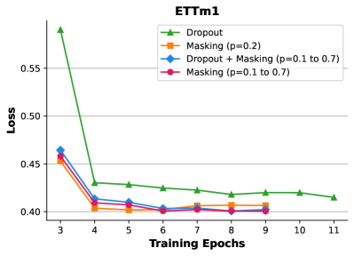
(a) ETTm1 with $T=720$

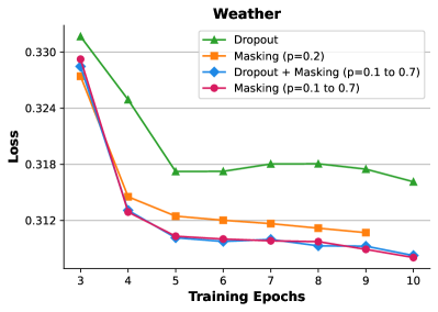
(b) Weather with $T=720$

Figure 7: Comparison of performance with query-adaptive masking with two different probabilities, dropout, and using both query-adaptive masking and dropout. The results of $p=0.1$ to $0.7$ indicate a probability masking that is linearly increased proportionally to the horizon predicted by the query.

Appendix C Detailed Explanation of Section 4.4

In this section, we provide the detailed results of experiments in Section 4.4. We first restate the formulation of two independent signals used in Section 4.4 as follows:

$${\mathbf{x}}(t) =\{x_{(t\bmod\tau)}\}^{\infty}_{t=1},\quad x_{i}\sim\mathcal{N}(0,1)\quad(i=0,1,\ldots,\tau-1),$$

$${\bm{y}}(t) =\begin{cases}+k&\text{if }t\equiv 0\pmod{S}\\ -k&\text{if }t\equiv\frac{1}{2}S\pmod{S}\end{cases},$$

We use the model parameters as follows: the patch length is 4 without overlapping, the decoder has 1 layer, and there are 2 attention heads. The signals ${\mathbf{x}}(t)$ and ${\bm{y}}(t)$ are defined with $\tau=24$, $S=8$, and $k=5$. The visualization of synthetic data is shown in Fig. 8. We utilize an input sequence length $L=48$ and a forecasting horizon $T=72$. This setup allows us to generate time series data with distinct periodic components.

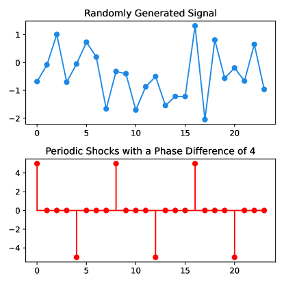
(a) Two input signals

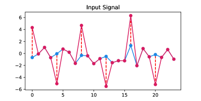
(b) Sum of two input signals

Figure 8: Visualization of input signals for toy experiment.

In the main paper, Fig. 5 displays a cross-attention score map between the input patch and the output patch derived from this experiment. The left figure presents the attention score of the first attention head, illustrating the model’s ability to detect shocks within the signal. The right figure more clearly demonstrates the periodicity of the signal. Given that the patch length and stride are both set to 4, each patch will contain exactly one shock value, either -5 or +5. This is because the shocks occur every 4 steps, alternating between positive and negative shocks. Consequently, the patch immediately preceding the current patch will contain a different shock, leading to lower attention scores due to the differing shock values. In contrast, patches that are an even number of steps before the current patch will contain the same type of shock, resulting in higher attention scores. These points are well illustrated in Fig. 5a, where the varying attention scores correspond to the presence of alternating shocks. This pattern helps to highlight the alternating shock signal within the data.

Additionally, if there is a correlation with the series preceding 24 steps, the patches that are 6 steps or multiples of 6 steps before the current patch will exhibit high attention scores due to the periodic nature of the signal ${\mathbf{x}}(t)$. The diagonal formation of the attention scores, which accurately follows a period of 24, is clearly depicted in Fig. 5b, highlighting the model’s capability to utilize fixed-period input patches to predict future outcomes. This periodic pattern ensures that the attention mechanism effectively captures the 24-step periodicity in ${\mathbf{x}}(t)$, reflecting the model’s ability to leverage this periodic information for more accurate predictions.

This experimental configuration provides a robust framework to evaluate how well our proposed model captures and interprets the underlying patterns in the data, specifically focusing on the alternating shock signal and the periodic nature of the normal signal. This dual emphasis on both the shock signal and the periodicity of the normal signal enhances the interpretability and predictive performance of the model, distinctly demonstrating how the model leverages periodic information to enhance prediction accuracy.

To push further, we reproduce the experiment of Fig. 6 with other datasets used in forecasting tasks. We illustrate the results of the Weather, Traffic, Electricity, ETTm2, ETTh1, and ETTh2 in Figures 9, 10, 11, 12, 13, and 14, respectively. For each figure, (a) represents the forecasting results, (b) shows the cross-attention score map, and (c) and (d) illustrate the two pairs with the highest attention scores. For all figures, our attention-based explanation successfully discovers similar periodic patterns. Therefore, we believe that our model has the potential to provide a clearer understanding of the mechanisms underlying forecasting predictions. We hope that future research will continue to explore and expand upon this foundation.

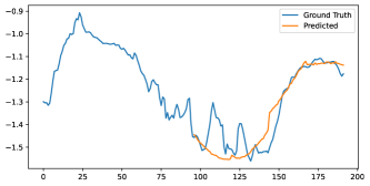
(a) Forecasting results

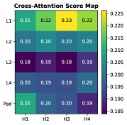
(b) Averaged score

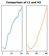
(c) L1-H2

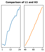
(d) L1-H3

Figure 9: Illustration of (a) forecasting result, (b) averaged cross-attention score, and (c,d) patches with the highest score on Weather. The score map is averaged from all the heads across layers.

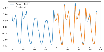
(a) Forecasting results

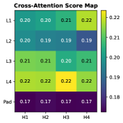
(b) Averaged score

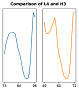
(c) L4-H3

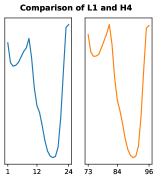
(d) L1-H4

Figure 10: Illustration of (a) forecasting result, (b) averaged cross-attention score, and (c,d) patches with the highest score on Traffic. The score map is averaged from all the heads across layers.

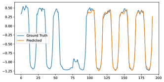
(a) Forecasting results

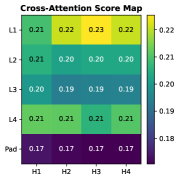
(b) Averaged score

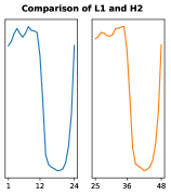
(c) L1-H2

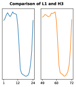
(d) L1-H3

Figure 11: Illustration of (a) forecasting result, (b) averaged cross-attention score, and (c,d) patches with the highest score on Electricity. The score map is averaged from all the heads across layers.

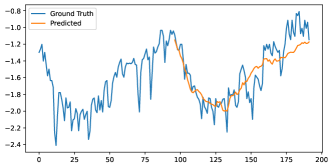
(a) Forecasting results

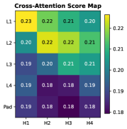
(b) Averaged score

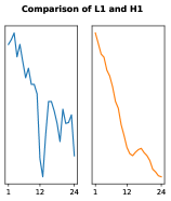
(c) L1-H1

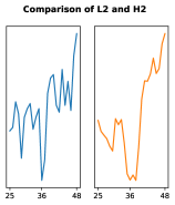
(d) L2-H2

Figure 12: Illustration of (a) forecasting result, (b) averaged cross-attention score, and (c,d) patches with the highest score on ETTm2. The score map is averaged from all the heads across layers.

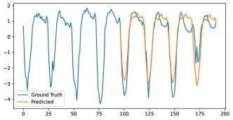
(a) Forecasting results

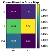
(b) Averaged score

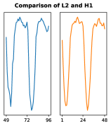
(c) L2-H1

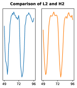
(d) L2-H2

Figure 13: Illustration of (a) forecasting result, (b) averaged cross-attention score, and (c,d) patches with the highest score on ETTh1. The score map is averaged from all the heads across layers.

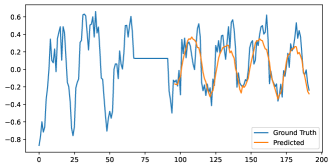
(a) Forecasting results

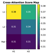
(b) Averaged score

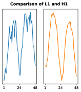
(c) L1-H1

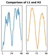
(d) L1-H2

Figure 14: Illustration of (a) forecasting result, (b) averaged cross-attention score, and (c,d) patches with the highest score on ETTh2. The score map is averaged from all the heads across layers.

References

- Chen et al. [2021] Chun-Fu Richard Chen, Quanfu Fan, and Rameswar Panda. Crossvit: Cross-attention multi-scale vision transformer for image classification. In Proceedings of the IEEE/CVF international conference on computer vision, pages 357–366, 2021.
- Chen et al. [2023] Si-An Chen, Chun-Liang Li, Sercan O Arik, Nathanael Christian Yoder, and Tomas Pfister. Tsmixer: An all-mlp architecture for time series forecast-ing. Transactions on Machine Learning Research, 2023.
- Das et al. [2024] Abhimanyu Das, Weihao Kong, Rajat Sen, and Yichen Zhou. A decoder-only foundation model for time-series forecasting. In International Conference on Machine Learning. PMLR, 2024.
- Devlin et al. [2019] Jacob Devlin, Ming-Wei Chang, Kenton Lee, and Lee Kristina. Bert: Pre-training of deep bidirectional transformers for language understanding. In Proceedings of NAACL-HLT, pages 4171–4186, 2019.
- Dosovitskiy et al. [2021] Alexey Dosovitskiy, Lucas Beyer, Alexander Kolesnikov, Dirk Weissenborn, Xiaohua Zhai, Thomas Unterthiner, Mostafa Dehghani, Matthias Minderer, Georg Heigold, Sylvain Gelly, Jakob Uszkoreit, and Neil Houlsby. An image is worth 16x16 words: Transformers for image recognition at scale. In International Conference on Learning Representations, 2021. URL https://openreview.net/forum?id=YicbFdNTTy.
- Ekambaram et al. [2023] Vijay Ekambaram, Arindam Jati, Nam Nguyen, Phanwadee Sinthong, and Jayant Kalagnanam. Tsmixer: Lightweight mlp-mixer model for multivariate time series forecasting. In Proceedings of the 29th ACM SIGKDD Conference on Knowledge Discovery and Data Mining, pages 459–469, 2023.
- Goswami et al. [2024] Mononito Goswami, Konrad Szafer, Arjun Choudhry, Yifu Cai, Shuo Li, and Artur Dubrawski. Moment: A family of open time-series foundation models. In International Conference on Machine Learning, 2024.
- Huang et al. [2016] Gao Huang, Yu Sun, Zhuang Liu, Daniel Sedra, and Kilian Q Weinberger. Deep networks with stochastic depth. In Computer Vision–ECCV 2016: 14th European Conference, Amsterdam, The Netherlands, October 11–14, 2016, Proceedings, Part IV 14, pages 646–661. Springer, 2016.
- Li et al. [2019] Shiyang Li, Xiaoyong Jin, Yao Xuan, Xiyou Zhou, Wenhu Chen, Yu-Xiang Wang, and Xifeng Yan. Enhancing the locality and breaking the memory bottleneck of transformer on time series forecasting. Advances in neural information processing systems, 32, 2019.
- Li et al. [2023] Zhe Li, Shiyi Qi, Yiduo Li, and Zenglin Xu. Revisiting long-term time series forecasting: An investigation on linear mapping. arXiv preprint arXiv:2305.10721, 2023.
- Liu et al. [2021] Shizhan Liu, Hang Yu, Cong Liao, Jianguo Li, Weiyao Lin, Alex X Liu, and Schahram Dustdar. Pyraformer: Low-complexity pyramidal attention for long-range time series modeling and forecasting. In International conference on learning representations, 2021.
- Liu et al. [2022] Yong Liu, Haixu Wu, Jianmin Wang, and Mingsheng Long. Non-stationary transformers: Exploring the stationarity in time series forecasting. Advances in Neural Information Processing Systems, 35:9881–9893, 2022.
- Liu et al. [2024] Yong Liu, Tengge Hu, Haoran Zhang, Haixu Wu, Shiyu Wang, Lintao Ma, and Mingsheng Long. itransformer: Inverted transformers are effective for time series forecasting. In The Twelfth International Conference on Learning Representations, 2024. URL https://openreview.net/forum?id=JePfAI8fah.
- Nie et al. [2023] Yuqi Nie, Nam H Nguyen, Phanwadee Sinthong, and Jayant Kalagnanam. A time series is worth 64 words: Long-term forecasting with transformers. In The Eleventh International Conference on Learning Representations, 2023. URL https://openreview.net/forum?id=Jbdc0vTOcol.
- Radford et al. [2018] Alec Radford, Karthik Narasimhan, Tim Salimans, Ilya Sutskever, et al. Improving language understanding by generative pre-training. 2018.
- Shazeer [2020] Noam Shazeer. Glu variants improve transformer. arXiv preprint arXiv:2002.05202, 2020.
- Strudel et al. [2021] Robin Strudel, Ricardo Garcia, Ivan Laptev, and Cordelia Schmid. Segmenter: Transformer for semantic segmentation. In Proceedings of the IEEE/CVF international conference on computer vision, pages 7262–7272, 2021.
- Van den Burg and Williams [2020] Gerrit JJ Van den Burg and Christopher KI Williams. An evaluation of change point detection algorithms. arXiv preprint arXiv:2003.06222, 2020.
- Vaswani et al. [2017] Ashish Vaswani, Noam Shazeer, Niki Parmar, Jakob Uszkoreit, Llion Jones, Aidan N Gomez, Łukasz Kaiser, and Illia Polosukhin. Attention is all you need. Advances in neural information processing systems, 30, 2017.
- Wang et al. [2022] Huiqiang Wang, Jian Peng, Feihu Huang, Jince Wang, Junhui Chen, and Yifei Xiao. Micn: Multi-scale local and global context modeling for long-term series forecasting. In The Eleventh International Conference on Learning Representations, 2022.
- Wang et al. [2024] Shiyu Wang, Haixu Wu, Xiaoming Shi, Tengge Hu, Huakun Luo, Lintao Ma, James Y. Zhang, and JUN ZHOU. Timemixer: Decomposable multiscale mixing for time series forecasting. In The Twelfth International Conference on Learning Representations, 2024. URL https://openreview.net/forum?id=7oLshfEIC2.
- Woo et al. [2023] Gerald Woo, Chenghao Liu, Doyen Sahoo, Akshat Kumar, and Steven Hoi. Learning deep time-index models for time series forecasting. In International Conference on Machine Learning, pages 37217–37237. PMLR, 2023.
- Wu et al. [2021] Haixu Wu, Jiehui Xu, Jianmin Wang, and Mingsheng Long. Autoformer: Decomposition transformers with auto-correlation for long-term series forecasting. Advances in neural information processing systems, 34:22419–22430, 2021.
- Wu et al. [2022] Haixu Wu, Tengge Hu, Yong Liu, Hang Zhou, Jianmin Wang, and Mingsheng Long. Timesnet: Temporal 2d-variation modeling for general time series analysis. In The eleventh international conference on learning representations, 2022.
- Yang et al. [2022] Chenglin Yang, Yilin Wang, Jianming Zhang, He Zhang, Zijun Wei, Zhe Lin, and Alan Yuille. Lite vision transformer with enhanced self-attention. In Proceedings of the IEEE/CVF Conference on Computer Vision and Pattern Recognition, pages 11998–12008, 2022.
- Zeng et al. [2023] Ailing Zeng, Muxi Chen, Lei Zhang, and Qiang Xu. Are transformers effective for time series forecasting? In Proceedings of the AAAI conference on artificial intelligence, volume 37, pages 11121–11128, 2023.
- Zhang et al. [2023] Haokui Zhang, Wenze Hu, and Xiaoyu Wang. Fcaformer: Forward cross attention in hybrid vision transformer. In Proceedings of the IEEE/CVF International Conference on Computer Vision, pages 6060–6069, 2023.
- Zhang and Yan [2022] Yunhao Zhang and Junchi Yan. Crossformer: Transformer utilizing cross-dimension dependency for multivariate time series forecasting. In The eleventh international conference on learning representations, 2022.
- Zhou et al. [2021] Haoyi Zhou, Shanghang Zhang, Jieqi Peng, Shuai Zhang, Jianxin Li, Hui Xiong, and Wancai Zhang. Informer: Beyond efficient transformer for long sequence time-series forecasting. In Proceedings of the AAAI conference on artificial intelligence, volume 35, pages 11106–11115, 2021.
- Zhou et al. [2022a] Tian Zhou, Ziqing Ma, Qingsong Wen, Liang Sun, Tao Yao, Wotao Yin, Rong Jin, et al. Film: Frequency improved legendre memory model for long-term time series forecasting. Advances in Neural Information Processing Systems, 35:12677–12690, 2022a.
- Zhou et al. [2022b] Tian Zhou, Ziqing Ma, Qingsong Wen, Xue Wang, Liang Sun, and Rong Jin. Fedformer: Frequency enhanced decomposed transformer for long-term series forecasting. In International conference on machine learning, pages 27268–27286. PMLR, 2022b.