Temporal Spiking Neural Networks with Synaptic Delay for Graph Reasoning

Abstract

Spiking neural networks (SNNs) are investigated as biologically inspired models of neural computation, distinguished by their computational capability and energy efficiency due to precise spiking times and sparse spikes with event-driven computation. A significant question is how SNNs can emulate human-like graph-based reasoning of concepts and relations, especially leveraging the temporal domain optimally. This paper reveals that SNNs, when amalgamated with synaptic delay and temporal coding, are proficient in executing (knowledge) graph reasoning. It is elucidated that spiking time can function as an additional dimension to encode relation properties via a neural-generalized path formulation. Empirical results highlight the efficacy of temporal delay in relation processing and showcase exemplary performance in diverse graph reasoning tasks. The spiking model is theoretically estimated to achieve $20\times$ energy savings compared to non-spiking counterparts, deepening insights into the capabilities and potential of biologically inspired SNNs for efficient reasoning. The code is available at https://github.com/pkuxmq/GRSNN.

1 Introduction

Spiking Neural Networks, inspired by the detailed dynamics of biological neurons, are recognized as more biologically plausible models for neural computation and are distinguished as the third generation of neural network models, owing to their advanced computational capabilities derived from spiking time (Maass, 1997). Unlike traditional Artificial Neural Networks, SNNs integrate neuronal dynamics using differential equations and leverage sparse spike trains in the temporal domain for information transition (Fig. 1a), enhancing the encoding of information in biological brains (Reinagel & Reid, 2000; Huxter et al., 2003) and exhibiting increased expressive power when incorporating delay variables (Maass, 1997). The utilization of sparse, event-based computation in SNNs facilitates energy-efficient operation on neuromorphic hardware with parallel in-/near-memory computing (Davies et al., 2018; Pei et al., 2019; Rao et al., 2022), making SNNs increasingly prominent as powerful and efficient neuro-inspired models in Artificial Intelligence (AI) applications (Rueckauer et al., 2017; Shrestha & Orchard, 2018; Roy et al., 2019; Bellec et al., 2020; Stöckl & Maass, 2021; Yin et al., 2021; Rao et al., 2022; Xiao et al., 2022; Li et al., 2023; Zhang et al., 2024). Despite these advancements, critical inquiries remain unresolved regarding the solution by SNNs for human-like graph-based reasoning of concepts or relations and an improved utilization of spiking time for information processing.

Symbolic and relational reasoning is a cornerstone of human intelligence and advanced AI capabilities (Kemp & Tenenbaum, 2008; Santoro et al., 2017; Rao et al., 2022; Nickel et al., 2015) and can often be formulated as graph reasoning with tasks like link prediction in knowledge graphs (Fig. 1b) (Nickel et al., 2015). For example, it can be evaluated by machine learning tasks of knowledge graph completion (Nickel et al., 2015) and inductive relation prediction (Yang et al., 2017; Teru et al., 2020), resembling humans’ ability to reason new relations between entities based on commonsense knowledge graphs or generalize relations to new analogous conditions. Investigating how underlying mechanisms of neural computation can realize this reasoning capability is pivotal for understanding human intelligence and advancing AI systems, as graph reasoning is important for extensive AI tasks such as knowledge graphs, recommendation systems, and drug or material design (Wang et al., 2023). While various machine learning methods, including path-based (Lao & Cohen, 2010; Yang et al., 2017; Sadeghian et al., 2019), embedding (Bordes et al., 2013; Yang et al., 2015; Sun et al., 2019), and Graph Neural Networks (Schlichtkrull et al., 2018; Vashishth et al., 2020; Teru et al., 2020; Zhu et al., 2021), have been proposed for graph reasoning tasks, the efficacy of bio-inspired models in achieving comparable performance remains largely unexplored. Existing attempts, such as entity embedding by spiking times of single neurons (Dold & Garrido, 2021; Dold, 2022) or in-context relational reasoning (Rao et al., 2022), have not addressed how reasoning paths can be propagated, especially with optimal utilization of temporal information at the network level, and have shown limitations in inductive generalization, interpretability, and performance in large knowledge graphs.

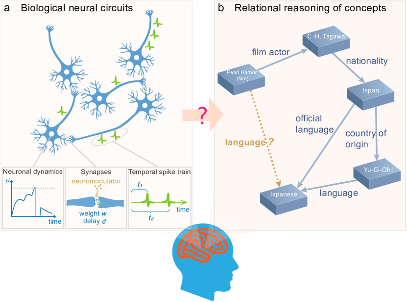
Figure 1: Depiction of spiking neural networks and knowledge graph reasoning. (a) A representation of biological neural circuits, showcasing spiking neurons, their inherent dynamics, synaptic interconnections, and the propagation of temporal spike trains. (b) The process of relational reasoning of concepts, exemplified through the link prediction task in knowledge graphs.

Moreover, the importance of spiking time in SNNs (Maass, 1997; Reinagel & Reid, 2000; Huxter et al., 2003) and its potential in AI applications necessitate further exploration. Many previous works have primarily focused on enhancing SNNs as energy-efficient alternatives to ANNs for tasks like image classification (Rueckauer et al., 2017; Shrestha & Orchard, 2018; Xiao et al., 2022), with an emphasis on spike counts. Efforts to leverage spiking time have explored encoding information for single neurons by the time to first spike (Mostafa, 2017; Comsa et al., 2020; Dold & Garrido, 2021), the interval between spikes (Dold, 2022), or adopting different weight coefficients at different times (Stöckl & Maass, 2021), and some have delved into temporal processing tasks like time series classification (Yin et al., 2021; Rao et al., 2022; Patiño-Saucedo et al., 2023; Hammouamri et al., 2024). However, more systematic utilization of synaptic delay at the network level and the coding principles embedded in neuronal spike trains are areas that warrant deeper investigation for better understanding and application of SNNs in extensive AI tasks.

In this work, we introduce Graph Reasoning Spiking Neural Network (GRSNN), a novel method allowing SNNs to adeptly solve knowledge graph reasoning tasks by leveraging synaptic delay to encode relational information. This method enables the temporal domain of SNNs to act as an additional dimension to process edge and path properties at the network level, offering a fresh perspective on temporal information processing and coding in SNNs.

We consider link prediction tasks of knowledge graphs and GRSNN is proposed as a neural generalization to the path formulation of graph algorithms, drawing inspiration from existing works (Aimone et al., 2021; Zhu et al., 2021). Path formulation is important to graph reasoning due to better interpretability and inductive generalization ability (Zhu et al., 2021; Yang et al., 2017; Sadeghian et al., 2019). We generalize the thought—SNNs can provide a parallelizable and efficient solution to traditional graph path tasks—into AI applications of graph reasoning. It can serve as a neural generalization of Dijkstra’s algorithm with learnable synaptic delays representing the properties of graph edges (also coupled with synaptic weights), enabling high-performance and interpretable solutions.

Experiments on diverse graph prediction tasks are conducted to assess the effectiveness of GRSNN. The results underscore the advantage of synaptic delay in encoding relation information in SNNs for competitive performance, revealing a potential mechanism of spiking neurons for knowledge reasoning, and demonstrate the efficiency of GRSNN by fewer parameters and spike computation, with a theoretical estimation indicating significant energy savings compared to non-spiking counterparts. These insights enhance our understanding of the role of neuro-inspired models in graph-based reasoning tasks, central to human intelligence, and emphasize the potential of the temporal domain of SNNs in developing energy-efficient solutions for graph-based AI applications.

2 Preliminaries

2.1 Spiking Neural Networks

SNNs are brain-inspired models comprising spiking neurons that communicate through temporal spike trains. In this work, we employ the current-based Leaky Integrate and Fire (current-based LIF) spiking neuron model, which can be equivalently represented using the Spike Response Model (SRM) form. In this model, each spiking neuron maintains a membrane potential $u$, integrating input spike trains according to the dynamics:

$$\small\tau_{m}\frac{du}{dt}=-(u(t)-u_{rest})+R\cdot I(t),\quad u(t)<V_{th},$$ (1)

where $I$ is the input current, $V_{th}$ is the threshold, $R$ is the resistance, and $\tau_{m}$ is the membrane time constant. When $u$ reaches $V_{th}$ at time $t^{f}$, a spike is emitted, and $u$ is reset to the resting potential $u=u_{rest}$, typically set to zero. The neuron’s output spike train is represented as $s(t)=\sum_{t^{f}}\delta(t-t^{f})$, using the Dirac delta function.

Neurons are interconnected through synapses with weight and delay (axonal or synaptic delay, for simplicity, we call synaptic delay in this paper). The model for input current is given by:

$$\small\tau_{c}\frac{dI_{i}}{dt}=-I_{i}(t)+\sum_{j}w_{ij}s_{j}(t-d_{ij})+b_{i},$$ (2)

where $w_{ij}$ and $d_{ij}$ are the synaptic weight and delay from neuron $j$ to neuron $i$, respectively, $b_{i}$ is a bias term representing background current, and $\tau_{c}$ is another time constant. Given the reset mechanism, the equivalent SRM form is:

$$u_{i}(t)= u_{rest}+\sum_{j}w_{ij}\int_{0}^{t}\kappa(\tau-d_{ij})s_{j}(t-\tau)\mathrm{d}\tau$$ (3)

$$+\int_{0}^{t}\nu(\tau)s_{i}(t-\tau)\mathrm{d}\tau,$$

with $\kappa(\tau)$ being the temporal kernel function for input spikes and $\nu(\tau)=-(V_{th}-u_{rest})e^{-\frac{\tau}{\tau_{m}}}$ representing the reset kernel. Assuming $\tau_{c}=\tau_{m}$, the input kernel becomes $\kappa(\tau)=\frac{R}{\tau_{m}}\cdot\tau e^{-\frac{\tau}{\tau_{m}}}$ for $\tau\geq 0$ and $\kappa(\tau)=0$ for $\tau<0$. Setting $R=e$, the kernel simplifies to $\kappa(\tau)=\frac{\tau}{\tau_{m}}e^{1-\frac{\tau}{\tau_{m}}}$, which is commonly used (Shrestha & Orchard, 2018).

In practice, we simulate SNNs using the discrete computational form of the current-based LIF model:

$$\small\left\{\begin{aligned} &I_{i}[t+1]=e^{-\frac{\Delta\tau}{\tau_{m}}}I_{i}[t]+\alpha\left(\sum_{j}w_{ij}s_{j}[t-d_{ij}]+b_{i}\right),\\ &u_{i}[t+1]=e^{-\frac{\Delta\tau}{\tau_{m}}}u_{i}[t](1-s_{i}[t])+I_{i}[t+1],\\ &s_{i}[t+1]=H(u_{i}\left[t+1\right]-V_{th}),\\ \end{aligned}\right.$$ (4)

where $H(x)$ is the Heaviside step function, $s_{i}[t]$ is the spike signal at discrete time step $t$, $\Delta\tau$ is the discretization interval, and $\alpha$ denote the coefficient $\frac{e\Delta\tau}{\tau_{m}}$.

Utilizing the equivalent SRM formulation and surrogate derivatives for the spiking function, gradients for parameters, including $w_{ij}$ and $d_{ij}$, can be computed through backpropagation over time (Shrestha & Orchard, 2018). Specifically, the non-differentiable term $\frac{\partial s_{i}[t]}{\partial u_{i}[t]}$ is substituted by surrogate derivatives of a smooth function, such as the derivative of the sigmoid function: $\frac{\partial s}{\partial u}=\frac{1}{a_{1}}\frac{e^{(V_{th}-u)/a_{1}}}{(1+e^{(V_{th}-u)/a_{1}})^{2}}$, with $a_{1}$ as a hyperparameter. The gradients are then calculated as $\frac{\partial\mathcal{L}}{\partial w_{ij}}=\sum_{t}\frac{\partial\mathcal{L}}{\partial s_{i}[t]}\frac{\partial s_{i}[t]}{\partial u_{i}[t]}\frac{\partial u_{i}[t]}{\partial w_{ij}}$ and $\frac{\partial\mathcal{L}}{\partial d_{ij}}=\sum_{t}\frac{\partial\mathcal{L}}{\partial s_{i}[t]}\frac{\partial s_{i}[t]}{\partial u_{i}[t]}\frac{\partial u_{i}[t]}{\partial r_{ij}[t]}\frac{\partial r_{ij}[t]}{\partial d_{ij}}$, where $r_{ij}[t]=\sum_{\tau=0}^{t}\kappa(\tau-d_{ij})s_{j}[t-\tau]$, and $\frac{\partial r_{ij}[t]}{\partial d_{ij}}=-\sum_{\tau=0}^{t}\dot{\kappa}(\tau-d_{ij})s_{j}[t-\tau]$ ($\dot{\kappa}$ denotes the derivative of the kernel $\kappa$). In a discrete setting, $\mathbf{d}_{ij}$ should be integers, and we employ the straight-through-estimator to train a quantized real-valued variable. For additional details, please refer to Appendix A. In this study, we primarily focus on parameters $w_{ij}$ and $d_{ij}$, leaving the exploration of heterogeneous neurons for future work.

2.2 Link Prediction of Graphs

We consider link prediction tasks of (knowledge) graphs. A knowledge graph is denoted by $\mathcal{G}=(\mathcal{V},\mathcal{E},\mathcal{R})$, with $\mathcal{V}$, $\mathcal{E}$, and $\mathcal{R}$ representing the sets of graph nodes, graph edges, and relation types, respectively. We also consider homogeneous graphs $\mathcal{G}=(\mathcal{V},\mathcal{E})$ as a special case with only one relation type. The task is to predict whether an edge of type $q$ exists between entities $x,y$ (Fig. 2a), and the common methods are to calculate or learn a pair representation $\mathbf{h}^{q}(x,y)$ for prediction, e.g., using paths between two nodes or embedding methods or GNNs, while we explore using SNNs. Many link prediction tasks are transductive, i.e., predicting new links on the training graph, and there is also the inductive setting where training and testing graphs have different entities but the same relation types.

2.3 Synaptic Delay for Traditional Graph Algorithms

Some previous works show that the synaptic delay of SNNs can be leveraged to solve traditional graph tasks, providing a parallelizable and efficient neuromorphic computing solution to graph algorithms (Aimone et al., 2021). For the traditional graph single-source shortest path problem, by assigning a neuron to each graph node and configuring the delay between neurons as the graph edge weight, SNNs can parallelly simulate Dijkstra’s algorithm. An example is shown in Fig. 2e if we decode the spike train of the target neuron by the time to first spike. We will generalize the thought—delays in SNNs can represent the properties of graph edges—to graph AI reasoning tasks with neural generalization and advanced temporal coding with multiple temporal spikes for diverse paths.

3 Graph Reasoning Spiking Neural Network

In this section, we introduce our graph reasoning spiking neural networks. We first introduce the overview of our model in Section 3.1. Then in Section 3.2, we demonstrate that GRSNN can be viewed as a generalized path formulation for graph reasoning. In Section 3.3, we discuss the comparison with graph neural networks. Finally, we introduce implementation details in Section 3.4.

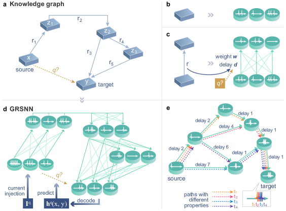
Figure 2: Schematic of GRSNN. (a) Illustration of the graph link prediction task. In GRSNN, (b) each graph entity node is associated with a cluster of spiking neurons, and (c) each relational edge corresponds to the synaptic connections between spiking neurons, with synaptic weight and delay. The weight can exhibit positive or negative values. The delay is contingent on the edge relation and query relation, representing the edge’s property and the neuromodulation from the task goal. (d) Visualization of GRSNN. To predict a link, a constant current, dependent on the query relation, is injected into the spiking neurons of the source node, initiating the propagation of spike trains. After a specific time interval, the spike trains emanating from the target node are decoded to predict the query relation. (e) Depiction of the temporal domain serving as an additional dimension to process the properties of edges and paths in a network with more propagation paths. In the demonstrated network under a simplified setting where each input spike triggers an output spike for neurons, a spike from the source neuron will lead to four spikes from the target neuron, whose time varies corresponding to four propagation paths with different integrated properties of edges represented by synaptic delay.

3.1 Model Overview

The outline of GRSNN is depicted in Fig. 2. Each graph node is assigned $n$ spiking neurons, representing each entity by a neuron population (Fig. 2b). Synaptic connections, corresponding to relation links between entities, are characterized by weight and delay between neuron groups (Fig. 2c). These synaptic properties, such as delay, are dependent on the graph edge relation and modulated by the query relation (task goal), allowing the integrated properties of paths to be reflected by the spiking time considering delays (Fig. 2e). Unlike SNNs for traditional graph tasks, we generalize the model to allow both positive and negative synaptic weights, acting as complementary transformations to learnable synaptic delays that are viewed as an additional dimension to process graph edges and paths.

For the link prediction task (Fig. 2d), a constant current $\mathbf{I}^{q}$ is injected to the spiking neurons of the source node $x$ for a given query $q$ between nodes $x$ and $y$, generating spike trains. The network then propagates these spikes, and a spike train $\mathbf{s}_{y}^{q}(t)$ from the target node $y$’s neurons is obtained after a time interval. A decoding function $D$ calculates the pair representation $\mathbf{h}^{q}(x,y)=D(\mathbf{s}_{y}^{q}(t))$ for link prediction, and we primarily utilize temporal coding $D(\mathbf{s}_{y}^{q}(t))=\left(\sum_{\tau}\lambda^{\tau}\mathbf{s}_{y}^{q}[\tau]\right)/\left(\sum_{\tau}\lambda^{\tau}\right)$, emphasizing early spiking time. This corresponds to the decoding for various path formulations (refer to Appendix B for more details).

3.2 GRSNN as Generalized Path Formulation

GRSNN serves as a neural generalization of the path formulation for graphs, allowing for the simultaneous consideration of all paths from a source node without the separate calculation of each one. Path formulation is important to graph reasoning due to better interpretability and inductive generalization ability (Zhu et al., 2021; Yang et al., 2017; Sadeghian et al., 2019). Traditional path-based algorithms calculate the pair representation between nodes $x$ and $y$ by considering paths from $x$ to $y$, formulated as a generalized accumulation of path representations (Zhu et al., 2021):

$$\small\mathbf{h}^{q}(x,y)=\bigoplus_{P\in\mathcal{P}_{xy}}\left(\bigotimes_{i=1}^{|P|}\mathbf{v}^{q}(e_{i})\right),\vspace{-1mm}$$ (5)

where $\mathcal{P}_{xy}$ is the set of paths from $x$ to $y$, $e_{i}$ is the $i$-th edge on a path $P$, and $\mathbf{v}^{q}(e_{i})$ is the edge representation (e.g., the transition probability of this edge). Various methods like Katz Index (Katz, 1953), Personalized PageRank (Page et al., 1999), and Graph Distance (Liben-Nowell & Kleinberg, 2007) follow this modeling.

In GRSNN, spike trains propagate over time, with spikes at different times simultaneously maintaining all paths from the source node. The spike train of $y$ is:

$$\mathbf{s}_{y}^{q}(t) =f\left(\left\{\mathbf{s}_{z}^{q}(t),\mathbf{w}_{z,y}^{q},\mathbf{d}_{z,y}^{q}|z\in\mathcal{N}(y)\right\}\right)$$ (6)

$$=\cdots=\overline{f}\left(\left\{\mathbf{s}_{x}^{q}(t),\{\mathbf{w}_{e_{i}}^{q},\mathbf{d}_{e_{i}}^{q}\}_{i=1}^{|P|}|P\in\mathcal{P}_{xy}\right\}\right),$$

where $f$ is the function of spiking neurons, $\mathbf{w}_{z,y}^{q}$ and $\mathbf{d}_{z,y}^{q}$ are synaptic weights and delays between nodes $z$ and $y$ given the query relation $q$, $\mathcal{N}(y)$ denotes the set of neighbors of $y$, and $\overline{f}$ denotes the general composite function for all paths. In some degenerated conditions, the time of a spike is the sum of edge delays on one path, allowing a decoding function $F$ to perform a general summation over all paths represented in the spike train. We show that, with specific settings, GRSNN can solve traditional path-based methods.

Proposition 3.1.

Katz Index, Personalized PageRank, and Graph Distance can be solved by GRSNN under specific settings.

The proof is detailed in Appendix B, focusing on the construction of appropriate delay and decoding functions. This proposition illustrates that GRSNN can degenerate to emulate traditional path-based algorithms. By employing parameterized synaptic delays for learnable edge representations, and additional parameters like synaptic weights for transformations in another dimension, GRSNN emerges as a neural generalization of the path formulation for graph reasoning. This sheds light on the capability of SNNs to execute neuro-symbolic computation on graph paths utilizing spiking time and synaptic delay. Furthermore, GRSNN, as a generalization of path formulation, extends its important applicability to inductive settings and reasoning path interpretations, distinguishing it from entity embedding methods.

3.3 Comparison with Graph Neural Networks

The introduced GRSNN bears a resemblance to the widely-used message-passing GNNs in machine learning, both propagating messages between interconnected nodes. However, notable distinctions exist.

First, GRSNN incorporates varied temporal synaptic delays in message passing, allowing for the encoding of relational information in spiking times with enhanced spatiotemporal processing. In contrast, GNNs uniformly propagate messages across all edges in each iteration. Second, GRSNN disseminates temporal spike trains throughout the network, as opposed to GNN’s real-valued activations. This not only facilitates the representation of multiple paths through diverse spiking times within a spike train but also promotes event-driven energy-efficient computation suitable for neuromorphic hardware. Moreover, while Zhu et al. (2021) interprets GNN as a neural counterpart to the Bellman-Ford algorithm, GRSNN is perceived as a neural generalization of Dijkstra’s algorithm. This parallel between artificial and brain-inspired neural networks in generalizing distinct classical algorithms for analogous objectives is intriguing.

Once the inherent differences are accounted for, GRSNN can also have a formulation analogous to GNNs. Specifically, at each discrete time step, every node (with spiking neurons) aggregates messages from neighbors. Assuming the sharing of synaptic weights across all edges, akin to GNNs, messages are represented by delayed spikes. The aggregation function then becomes a synthesis of the summation of all messages, a linear transformation, and the spike generation with neuronal dynamics of spiking neurons. Thus, for every node $z$, the following holds:

$$\small\left\{\begin{aligned} &\mathbf{I}^{q}_{z}[t+1]=e^{-\frac{\Delta\tau}{\tau_{m}}}\mathbf{I}^{q}_{z}[t]+\alpha\left(\mathbf{W}\sum_{k\in\mathcal{N}(z)}\mathbf{s}^{q}_{k}[t-\mathbf{d}^{q}_{r}]+\mathbf{b}\right),\\ &\mathbf{u}^{q}_{z}[t+1]=e^{-\frac{\Delta\tau}{\tau_{m}}}\mathbf{u}^{q}_{z}[t](1-\mathbf{s}^{q}_{z}[t])+\mathbf{I}^{q}_{z}[t+1]+\mathbbm{1}_{z=x}\mathbf{I}^{q},\\ &\mathbf{s}^{q}_{z}[t+1]=H(\mathbf{u}^{q}_{z}[t+1]-V_{th}).\\ \end{aligned}\right.$$ (7)

Here, $r$ signifies the relation from node $k$ to node $z$, $\mathbf{s}^{q}_{k}[t-\mathbf{d}^{q}_{r}]$ represents the vector of spikes with associated delays $\mathbf{d}^{q}_{r}$, and $\mathbbm{1}_{z=x}$ is an indicator for the current injection to the source node. The time steps can be viewed as the layers of GNNs, with shared weights and delays for all time steps. Consequently, the inference time and space complexity of GRSNN align closely with those of GNNs, except that they are proportional to the number of discrete time steps instead of GNN’s layer number.

3.4 Implementation Details

Model Detail

In practice, our models predominantly adhere to Eq. 7. The set of learnable parameters encompasses $\mathbf{W}$ and $\mathbf{b}$, symbolizing a shared linear transformation of synaptic weights, and $\mathbf{d}^{q}_{r}$, denoting the delay between the spiking neurons of two nodes, contingent on their relation $r$ and the query relation $q$. Additionally, $\mathbf{r}$ signifies the embedding of relations, utilized for both current injection ($\mathbf{I}^{q}=\mathbf{r}^{q}$) and the ultimate link prediction with a parameterized function to predict links based on $\mathbf{h}^{q}(x,y)$ and $\mathbf{r}^{q}$. To differentiate the varying contributions of a relation (edge) in forecasting different query relations, we align with previous studies (Zhu et al., 2021) to parameterize the edge representation of relation $r$ as a linear function over the query relation. This is then processed through a sigmoid function with a bound scale $\beta$ to serve as positive delays, i.e., $\mathbf{d}^{q}_{r}=\beta\sigma(\mathbf{W}_{r}\mathbf{r}^{q}+\mathbf{b}_{r})$. In the context of homogeneous graphs characterized by a singular relation, this simplifies to $\mathbf{d}^{q}_{r}=\beta\sigma(\mathbf{b}_{r})$. It undergoes quantization and is trained by the straight-through-estimator. Post-learning, it can be archived in a look-up table, obviating the need for nonlinear computations. This can be analogous to neuromodulation with a superior signal delineating the task objective.

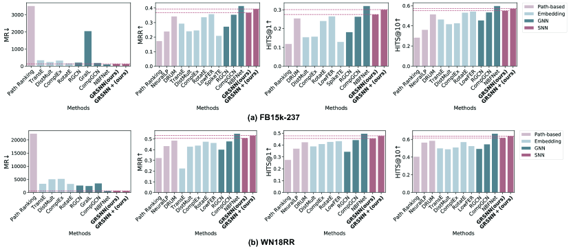
Figure 3: Results of Transductive Knowledge Graph Completion on FB15k-237 and WN18RR. Lower values are preferable for MR, while higher values are desirable for MRR, HITS@1, and HITS@10. Detailed values can be found in Section F.1.

Link Prediction Detail

In line with prevalent practices for link prediction, the objective is to ascertain the likelihood of a triplet $(x,q,y)$, consisting of the source node, query relation, and target node. The procedure of our model to deduce a triplet $(x,q,y)$ commences with the propagation of spike trains across the graph to secure the pair representation $\mathbf{h}^{q}(x,y)$, and subsequently, the likelihood score is computed by a parameterized function $g$ given $\mathbf{h}^{q}(x,y)$, consistent with prior studies (Zhu et al., 2021). More details can be found in Section E.1. The overarching procedure aligns with the conventional graph reasoning paradigm, with our primary focus being on the pivotal step of acquiring the pair representation through SNN propagation.

Regarding the training procedure, we adhere to the methodologies of preceding works (Bordes et al., 2013; Sun et al., 2019; Zhu et al., 2021), generating negative samples by corrupting one entity in a positive triplet. Please refer to Section E.1 for more details.

4 Experiments

In this section, we conduct experiments on transductive knowledge graph completion, inductive knowledge graph relation prediction, and homogeneous graph link prediction to evaluate the proposed GRSNN model. For knowledge graphs, we consider the commonly used FB15k-237 (Toutanova & Chen, 2015) and WN18RR (Dettmers et al., 2018) with the standard transductive splits and inductive splits (Teru et al., 2020). For homogeneous graphs, we consider Cora, Citeseer, and PubMed (Sen et al., 2008). The train/valid/test ratio of edges is 85:5:10 following the common practice, and the statistics of datasets can be found in Appendix D.

For evaluation of knowledge graph completion, we adhere to the filtered ranking protocol (Bordes et al., 2013), ranking a test triplet $(x,q,y)$ against all unseen negative triplets and report Mean Rank (MR), Mean Reciprocal Rank (MRR), and HITS@N. For inductive knowledge graph relation prediction, the evaluation adheres to the protocols outlined in the literature (Teru et al., 2020), where 50 negative triplets are drawn for each positive one using the filtered ranking, and the results are reported as HITS@10. For homogeneous graph link prediction, we follow Kipf & Welling (2016); Zhu et al. (2021) to compare the positive edges against the same number of negative edges, and the results are quantified using Area Under the Receiver Operating Characteristic Curve (AUROC) and Average Precision (AP).

More experimental details can be found in Section E.3.

4.1 Transductive Knowledge Graph Completion

We initiate our evaluation with experiments on transductive knowledge graph completion to assess the efficacy of GRSNN. This task, illustrated in Section E.2, involves predicting unseen relations between two existing entities in a knowledge graph and serves as a standard for assessing graph reasoning link prediction.

Table 1: Results of knowledge graph completion on FB15k-237 by SNNs with different methods to represent relation information. For MR, the lower the better. For MRR, HITS@1, HITS@3, and HITS@10, the higher the better.

Method	MR$\downarrow$	MRR$\uparrow$	H@1$\uparrow$	H@3$\uparrow$	H@10$\uparrow$
None	396	0.204	0.119	0.226	0.380
Synaptic weight	197	0.311	0.220	0.343	0.491
Synaptic delay	139	0.368	0.275	0.407	0.551

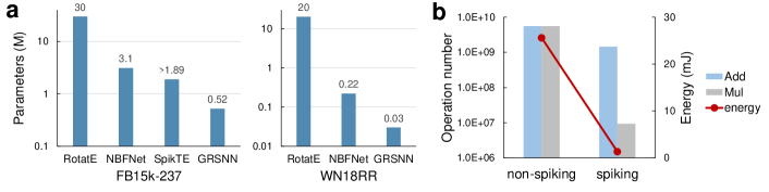
Figure 4: Analytical Results for GRSNN. (a) Log-scale comparison of the parameter quantities across different methods, demonstrating the enhanced parameter efficiency of GRSNN. (b) Theoretical estimations of the number of ADD and MUL operations (log scale) and energy consumption on FB15k-237. GRSNN can achieve approximately $20\times$ energy reduction compared to its non-spiking counterpart.

Advantage of synaptic delay

We investigate the role of synaptic delay in encoding relational information for reasoning, illustrated in Table 1. Our experiments contrast two baselines. The first baseline does not encode edge relations, focusing solely on the existence of edges. The second encodes edge relations with an additional relation-dependent term in synaptic weights, eschewing synaptic delay, reminiscent of the DistMult message function in GNN. More details are provided in the Section E.3. The results, presented in Table 1, highlight that synaptic delay significantly excels over the baselines, accentuating the merits of incorporating temporal processing with delays in bio-inspired models for effective relational reasoning.

Comparison with prevalent machine learning methods

We juxtapose the performance of our bio-inspired GRSNN with various machine learning methods, including path-based, embedding, and GNN methods, as depicted in Fig. 3, to underscore its efficacy in knowledge graph reasoning. We derive the results of preceding methods (Zhu et al., 2021; Vashishth et al., 2020; Dold, 2022). In essence, GRSNN secures competitive results, surpassing the majority of machine learning methods across all metrics, thereby attesting to the effectiveness of bio-inspired models in solving human-like advanced knowledge reasoning tasks. NBFNet attains superior performance by employing numerous GNN tricks that we deliberately omitted to preserve the inherent properties of SNNs. If we further integrate some techniques (refer to Section E.3), our model, denoted as GRSNN+ in Fig. 3, also achieves a better performance. Note that the proposed GRSNN prioritizes bio-plausibility, delivering promising performance with augmented efficiency, as will be analyzed in the following.

4.2 Analysis Results

Parameter amount

Fig. 4a contrasts the parameter quantities of several representative methods, highlighting the notable parameter efficiency of GRSNN in achieving competitive performance compared to other methods.

Theoretical estimation of energy

GRSNN leverages the energy efficiency inherent to SNNs through spike-based computation. On the test set of FB15k-237, the model exhibits a spike rate—the average spike count per discrete time step—of approximately 0.258. This translates to roughly a $4\times$ reduction in synaptic operations compared to equivalent real-valued neural networks. Given that spikes necessitate only Accumulate (AC) operations as opposed to Multiply-and-Accumulate (MAC) operations, there is a substantial reduction in energy costs, as evidenced by the energy consumption of 32-bit FP MAC and AC operations on a 45 nm CMOS processor being 4.6 pJ and 0.9 pJ, respectively (Horowitz, 2014). Fig. 4b provides a concise theoretical estimation of the number of addition and multiplication operations and the associated energy requirements, with the multiplication in SNNs arising due to leaky neuronal dynamics (please refer to Section E.3 for calculation details). Based on these estimations, a potential $20\times$ energy reduction is foreseeable, and under certain conditions where AC can be $31\times$ cheaper than MAC (Yin et al., 2021; Horowitz, 2014), this could extend to around $100\times$.

Note that there can also be costs from synaptic delay. We consider the Ring Buffer as a potential implementation, which is commonly used by digital neuromorphic platforms and analyzed (Patiño-Saucedo et al., 2023). The additional energy overhead will account for an extremely small proportion of energy—it is estimated as 0.004 mJ, while the energy for synaptic operations estimated above is 1.337 mJ (please refer to Section E.3 for calculation details), and this conclusion is consistent with Patiño-Saucedo et al. (2023). Therefore, the costs of synaptic delay do not affect the substantial energy efficiency.

More spike rate statistics on different datasets or tasks are presented in Table 2, showing that spikes are even sparser on other datasets or tasks introduced in the following. This underscores the substantial potential of GRSNN in enhancing energy efficiency by one to two orders of magnitude.

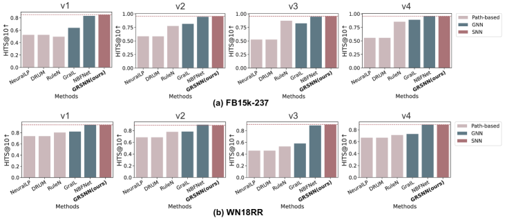
Figure 5: Results of Inductive Relation Prediction on FB15k-237 and WN18RR. v1-v4 correspond to the four standard versions of inductive splits. Detailed values can be found in Section F.1.

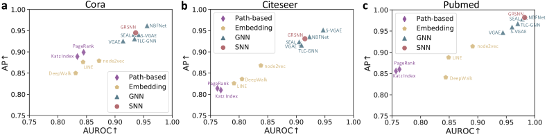
Figure 6: Results of Homogeneous Graph Link Prediction on Cora, Citeseer, and PubMed. Detailed values are in Section F.1.

Table 2: More spike rate statistics on different datasets.

Trans. Know. Graph Compl.		Induc. Relat. Pred.								Homo. Graph Link Pred.
FB15k-237	WN18RR	FB. v1	FB. v2	FB. v3	FB. v4	WN. v1	WN. v2	WN. v3	WN. v4	Cora	CiteSeer	PubMed
0.258	0.191	0.176	0.189	0.257	0.245	0.175	0.165	0.172	0.149	0.082	0.074	0.189

Interpretability

To demonstrate the interpretability of GRSNN as neural-generalized path formulation, in Section F.2, we visualize the reasoning paths for the final predictions of several examples, based on edge and path importance, determined by the gradient of the prediction w.r.t. edges, and beam search for paths of higher importance (refer to Section E.3 for details). Results show that GRSNN is adept at discerning relation relevances and exploiting transitions and analogs.

More analysis results such as the impact of temporal discretization steps and the impact of neuron number and parameter amount are in Appendix F.

4.3 Inductive Relation Prediction

Experiments are also conducted on inductive relation prediction to assess the efficacy of GRSNN. Unlike the transductive setting, which focuses on predicting new links within the training knowledge graph, inductive prediction strives to extrapolate the ability to predict relations from the training graph to a distinct testing graph. This testing graph encompasses different entities but retains the same relation types, as illustrated in Section E.2, demonstrating the ability to generalize relational reasoning to new conditions. Traditional entity embedding methods falter under this condition, whereas GRSNN, being a generalized form of path formulation, adeptly manages it.

The outcomes, depicted in Fig. 5, reveal that GRSNN surpasses the performance of most machine learning methods in inductive settings, underscoring its proficiency in generalizing reasoning to new entities. The spike rate statistics in Table 2 also indicate the potential for energy efficiency.

4.4 Homogeneous Graph Link Prediction

We also assess the GRSNN in the context of link prediction tasks for standard homogeneous graphs, illustrating its versatility across diverse application domains. Homogeneous graphs are essentially a subset of knowledge graphs, characterized by a singular type of relation, i.e., the presence of graph edges, and are ubiquitously observed. In such instances, the representation of edges remains consistent across the graph, and the GRSNN primarily leverages the information pertaining to graph distance in spiking time, as opposed to relation-specific information.

The results shown in Fig. 6 reveal that GRSNN manifests competitive performance in comparison to other proficient machine learning models, underscoring its efficacy. The sparse spike rates presented in Table 2 further highlight the efficiency potential.

5 Discussion and Conclusion

This study demonstrates the potential of bio-inspired SNNs in addressing graph reasoning through the innovative use of synaptic delay and spiking time. We introduced GRSNN, a model that employs synaptic delays to encode relation information of graph edges and utilizes the temporal domain as an additional dimension for processing graph path properties. This approach can be perceived as a neural generalization of the path formulation with better inductive generalization ability and interpretability. It provides insights into the capabilities of networks with biological neuron models to efficiently facilitate neuro-symbolic reasoning in tasks central to human intelligence, such as relational reasoning of concepts. Additionally, it explores the enhanced role that spiking time can play in AI applications. The promising performance and substantial theoretical energy efficiency of our model underscore the potential of SNNs in a wider array of applications such as efficient reasoning.

Our approach to temporal coding of spike trains assigns varying weights to different times, which is similar to the methodology in Stöckl & Maass (2021) but in our model, earlier spikes are designed to receive higher weights, which also integrates concepts from the time to first spike paradigm (Mostafa, 2017). Distinct to these works, our focus extends beyond individual neuron temporal coding to encompass the network level, allowing spiking time to integrate path properties during network propagation, and enabling multiple spikes to represent diverse paths globally. Unlike prior studies on traditional graph algorithms (Aimone et al., 2021), which primarily target the shortest path task, our work delves into the multifaceted realm of graph AI tasks with multiple temporal spikes for diverse paths. Together, our work offers a fresh perspective on temporal information processing in SNNs.

This study marks an initial exploration of utilizing SNNs for graph reasoning, leveraging the temporal domain, and opens avenues for numerous future directions. First, the reliance on discrete simulation and backpropagation through time for training SNNs is resource-intensive, especially for long simulation times with small discrete intervals. Therefore, this work primarily considers $T=10$ discrete time steps, which could sacrifice more precise temporal information. Enhancements in simulation or training methodologies at hardware/coding/algorithm levels may yield improved results given more accurate temporal information. Additionally, the exploration of online training methods conducive to on-chip learning of SNNs (Bellec et al., 2020; Xiao et al., 2022) for learning synaptic delays may offer insights into efficient and more biologically plausible learning of our model. Second, to fulfill the properties of SNNs, many advanced GNN strategies may not be incorporated, such as intricate message and aggregate functions and elaborate network structures. The investigation of SNN-compatible strategies may potentially bridge the performance gap, e.g., heterogeneous neurons and different neuron dynamics may provide more powerful computational properties (Chakraborty & Mukhopadhyay, 2023; Bellec et al., 2018). Last, given the prevalence of graph tasks in AI applications, future studies could delve into wider applications of graph reasoning such as drug or material design, investigating the potential of bio-inspired models for efficient applications.

In conclusion, our study illustrates the capability of brain-inspired SNNs in efficient symbolic graph reasoning, emphasizing the enhanced role of the temporal domain. Given their neuromorphic attributes, SNNs are poised to achieve substantial energy efficiency and high parallelism on spike-based neuromorphic hardware. It is our aspiration that this research serves as a catalyst for deeper insights and wider applications of biologically inspired efficient SNNs.

Impact Statement

This paper presents work whose goal is to advance the field of Machine Learning. There are many potential societal consequences of our work, none which we feel must be specifically highlighted here.

Appendix A Training Spiking Neural Networks

As introduced in Section 2.1, the models for membrane potential and current are described by the following equations:

$$\small\tau_{m}\frac{du}{dt}=-(u(t)-u_{rest})+R\cdot I(t),\quad u(t)<V_{th},$$ (8)

$$\small\tau_{c}\frac{dI_{i}}{dt}=-I_{i}(t)+\sum_{j}w_{ij}s_{j}(t-d_{ij})+b_{i},$$ (9)

and the equivalent SRM formulation is:

$$\small u_{i}(t)=u_{rest}+\sum_{j}w_{ij}\int_{0}^{t}\kappa(\tau-d_{ij})s_{j}(t-\tau)\mathrm{d}\tau+\int_{0}^{t}\nu(\tau)s_{i}(t-\tau)\mathrm{d}\tau.$$ (10)

Let $\mathcal{L}$ denote the loss based on the spikes of neurons. With the SRM formulation, the gradients for $w_{ij}$ and $d_{ij}$ can be calculated as follows:

$$\frac{\partial\mathcal{L}}{\partial w_{ij}}=\int_{0}^{T}\delta_{i}(t)\frac{\partial s_{i}(t)}{\partial u_{i}(t)}\left(\int_{0}^{t}\kappa(\tau-d_{ij})s_{j}(t-\tau)\mathrm{d}\tau\right)\mathrm{d}t,$$ (11)

$$\frac{\partial\mathcal{L}}{\partial d_{ij}}=\int_{0}^{T}\delta_{i}(t)\frac{\partial s_{i}(t)}{\partial u_{i}(t)}w_{ij}\left(-\int_{0}^{t}\dot{\kappa}(\tau-d_{ij})s_{j}(t-\tau)\mathrm{d}\tau\right)\mathrm{d}t,$$ (12)

where $\delta_{i}(t)$ is the gradient for $s_{i}(t)$ and can be recursively calculated by backpropagation through time as:

$$\delta_{i}(t)=\frac{\partial\mathcal{L}}{\partial s_{i}(t)}+\int_{t}^{T}\left(\sum_{j}\delta_{j}(\tau)\frac{\partial s_{j}(\tau)}{\partial u_{j}(\tau)}\frac{\partial u_{j}(\tau)}{\partial s_{i}(t)}+\delta_{i}(\tau)\frac{\partial s_{i}(\tau)}{\partial u_{i}(\tau)}\frac{\partial u_{i}(\tau)}{\partial s_{i}(t)}\right)\mathrm{d}\tau,$$ (13)

and $\dot{\kappa}(\cdot)$ represents the derivative of $\kappa(\cdot)$.

In practice, we simulate SNNs using the discrete computational form of the current-based LIF model:

$$\small\left\{\begin{aligned} &I_{i}[t+1]=\exp\left(-\frac{\Delta\tau}{\tau_{c}}\right)I_{i}[t]+\alpha\left(\sum_{j}w_{ij}s_{j}[t-d_{ij}]+b_{i}\right),\\ &u_{i}[t+1]=\exp\left(-\frac{\Delta\tau}{\tau_{m}}\right)u_{i}[t](1-s_{i}[t])+I_{i}[t+1],\\ &s_{i}[t+1]=H(u_{i}[t+1]-V_{th}).\\ \end{aligned}\right.$$ (14)

The gradients of $\delta_{i}(t)$ and $\frac{\partial\mathcal{L}}{\partial w_{ij}}$ can be calculated using the standard backpropagated automatic differentiation framework in deep learning libraries, based on the above formulation. The spiking function is non-differentiable, and $\frac{\partial s_{i}[t]}{\partial u_{i}[t]}$ can be replaced by a surrogate derivative (Shrestha & Orchard, 2018). We consider the derivative of the sigmoid function:

$$\small\frac{\partial s}{\partial u}=\frac{1}{a_{1}}\frac{e^{(V_{th}-u)/a_{1}}}{(1+e^{(V_{th}-u)/a_{1}})^{2}},$$ (15)

where we take $a_{1}=0.25$.

The automatic differentiation of the above formulation cannot directly handle $\frac{\partial\mathcal{L}}{\partial d_{ij}}$. We rewrite it in the discrete setting as:

$$\small\frac{\partial\mathcal{L}}{\partial d_{ij}}=\sum_{t}\delta_{i}[t]\frac{\partial s_{i}[t]}{\partial u_{i}[t]}w_{ij}\left(-\sum_{\tau=0}^{t-1}\dot{\kappa}[\tau-d_{ij}]s_{j}[t-1-\tau]\right).$$ (16)

We can integrate this into the automatic differentiation by tracking the trace ${tr}_{ij}[t]=-\sum_{\tau=0}^{t}\dot{\kappa}[\tau-d_{ij}]s_{j}[t-\tau]$ and calculating gradients based on it and the error backpropagated to $s_{j}[t-d_{ij}]$. In the discrete setting, $d_{ij}$ should be an integer index. We quantize it in the forward simulation and calculate gradients using the straight-through-estimator.

As described in Section 2.1, we consider $\tau_{c}=\tau_{m},R=e$ and the input kernel is $\kappa(\tau)=\frac{e\tau}{\tau_{m}}\exp\left(-\frac{\tau}{\tau_{m}}\right)$ for $\tau\geq 0$ and $\kappa(\tau)=0$ for $\tau<0$. Then, $\dot{\kappa}(\tau)=\frac{e}{\tau_{m}}\left(1-\frac{\tau}{\tau_{m}}\right)\exp\left(-\frac{\tau}{\tau_{m}}\right)$ for $\tau\geq 0$. In the discrete setting of the current-based LIF model, $\kappa$ is better described as $\kappa[\tau]=\alpha(\tau+1)\exp(-\frac{\tau}{\tau_{m}/\Delta\tau}),\tau\geq 0$ (where $\alpha=\frac{e}{\tau_{m}/\Delta\tau}$). Correspondingly, we take $\dot{\kappa}[\tau]=\alpha\left(1-\frac{\tau+1}{\tau_{m}/\Delta\tau}\right)\exp\left(-\frac{\tau}{\tau_{m}/\Delta\tau}\right)$ and calculate the trace ${tr}_{ij}$ based on it.

Appendix B Proof of Proposition 3.1

Proposition B.1.

Katz Index, Personalized PageRank, and Graph Distance can be solved by GRSNN under specific settings.

Proof.

We first introduce more details of Katz Index, Personalized PageRank, and Graph Distance. As described in Section 3.2, traditional path-based algorithms for graphs calculate the pair representation between nodes $x,y$ by considering paths from $x$ to $y$, and this can be formulated as a generalized accumulation of path representations (denoted as $\otimes$) with a commutative summation operator (denoted as $\oplus$):

$$\small\mathbf{h}^{q}(x,y)=\bigoplus_{P\in\mathcal{P}_{xy}}\left(\bigotimes_{i=1}^{|P|}\mathbf{v}^{q}(e_{i})\right),$$ (17)

where $\mathcal{P}_{xy}$ is the set of paths from $x$ to $y$, $e_{i}$ is the $i$-th edge on a path $P$, and $\mathbf{v}^{q}(e_{i})$ is the representation of the edge (e.g., the transition probability of this edge). Katz Index is a path formulation with $\oplus=+,\otimes=\times,\mathbf{v}^{q}(e)=\beta$, Personalized PageRank is with $\oplus=+,\otimes=\times,\mathbf{v}^{q}(e)=1/d_{out}(z)$ (where $d_{out}(z)$ is the output degree of the start node $z$ of edge $e$), and Graph Distance is with $\oplus=\min,\otimes=+,\mathbf{v}^{q}(e)=1$.

We examine these three distinct settings:

(1) Graph Distance: In this setting, each graph node is assigned one spiking neuron, and neurons are connected if there exists a graph edge between them, with all synaptic weights and thresholds set to $1$. Consequently, each input spike to a neuron will trigger an output spike. The synaptic delay of each edge is set as the corresponding positive graph edge length, allowing the propagation of spikes along edges to accumulate edge length into time. By initiating a spike from the source node at time $0$, GRSNN propagates spikes throughout the network, and the time to the first spike of each node represents the shortest distance to the source node. Utilizing the decoding function of the spike train from the target node as the first spiking time allows us to compute the graph distance.

(2) Katz Index: The Katz Index necessitates the accumulative multiplication of edge representations. By applying the log operation, this multiplication can be transformed into accumulation. For an edge representation $\beta\in(0,1)$ of Katz Index, corresponding to an attenuation factor, the synaptic delay is set as $d=-\log\beta$ (potentially scaled). For a spiking time $t$, $10^{-t}$ represents the accumulative multiplication of edge representations in the path. To sum over all paths, the number of paths during spike propagation must be maintained. A single spiking neuron is insufficient for this task as it will only generate one output spike when multiple paths simultaneously propagate to the same node. This limitation can be addressed by employing multiple spiking neurons, assigning $N$ spiking neurons to each graph node, with thresholds set as $1,2,\cdots,N$. Neurons connected by graph edges have synaptic weights of $1$ and delays as described above. The time and number of spikes of each node correspond to different paths from the source node. After sufficient propagation time, the decoding function of the spike train from the target node is defined as $D(\mathbf{s}(t))=\sum_{\tau}10^{-\tau}\left(\sum_{i}s_{i}[\tau]\right)$, enabling the computation of the Katz Index.

(3) Personalized PageRank: This is analogous to the Katz Index, with the edge representation being the transition probability $1/d_{out}(z)\in(0,1)$. The synaptic delay is similarly set as $d=-\log(1/d_{out}(z))$ (or with a scale). Thus, Personalized PageRank can be computed similarly to the Katz Index.

∎

Remark B.2.

The crux of the proof revolves around the construction of appropriate synaptic delays and decoding functions. As illustrated in the construction, distinct temporal coding methods naturally arise for varying path formulations. In many scenarios, the significance of edge representations in knowledge graphs can be interpreted as learnable probabilities, making the accumulative multiplication setting (as in Katz Index and Personalized PageRank) particularly advantageous. This results in the adoption of temporal coding in our experiments in the main text, assigning different weights to different spikes, represented as $D(\mathbf{s}_{y}^{q}(t))=\frac{\sum_{\tau}\lambda^{\tau}\mathbf{s}_{y}^{q}[\tau]}{\sum_{\tau}\lambda^{\tau}}$, except a constant factor. A notable distinction is that, instead of a straightforward summation across different neurons, we derive the pair representation as a vector of different neurons. Subsequently, the likelihood is computed using a learnable function $g$, aligning with the prevalent approaches in graph reasoning methods (refer to Section 3.4). This approach also serves as a broader generalization of the formulation in the construction.

Appendix C Related Work

Spiking Neural Networks Recent works mainly study SNNs as energy-efficient alternatives to ANNs by converting ANNs to SNNs for object recognition (Rueckauer et al., 2017; Stöckl & Maass, 2021; Li et al., 2021; Meng et al., 2022b) and natural language classification (Lv et al., 2023), or direct training SNNs (with surrogate gradients or other methods) for audio or visual perception (Shrestha & Orchard, 2018; Fang et al., 2021; Xiao et al., 2021; Meng et al., 2022a; Xiao et al., 2024), time series classification (Yin et al., 2021; Rao et al., 2022), seizure detection (Zhang et al., 2024), graph classification (Zhu et al., 2022; Li et al., 2023), etc. Most of them focus on spike counts and hardly leverage the important temporal dimension. Some works explore temporal encoding for single neurons (Mostafa, 2017; Comsa et al., 2020; Zhou et al., 2021; Stöckl & Maass, 2021), or utilizing spiking time for feature binding (Zheng et al., 2022), but how synaptic delay with temporal coding at the network level can be systematically utilized is rarely considered. Patiño-Saucedo et al. (2023) and Hammouamri et al. (2024) learn delays for time series tasks, and Yan et al. (2024) learn delays in network structure design, but they not consider temporal coding for graph tasks. Some works attempt to use SNNs for relational reasoning in knowledge graphs with entity embedding based on spiking times (Dold & Garrido, 2021; Dold, 2022) or population coding combined with reward-modulated STDP (Fang et al., 2022). They do not consider reasoning paths with synaptic delay and temporal coding, and are limited in inductive generalization and interoperability considering the entity embedding method as well as poor performance in large knowledge graphs. Differently, our novel method is the first to demonstrate the advantage of delays to represent relations with promising performance on real transductive and inductive (knowledge) graphs.

Graph Reasoning  Graph link prediction is a fundamental graph reasoning task, typically in the context of knowledge graph reasoning. Popular methods include three paradigms: path-based, embedding, and graph neural networks (Zhu et al., 2021). Path-based methods predict links based on paths from the source node to the target node, e.g., the weighted count of paths in homogeneous graphs (Katz, 1953; Page et al., 1999; Liben-Nowell & Kleinberg, 2007) or paths with learned probabilities or representations in knowledge graphs (Lao & Cohen, 2010; Yang et al., 2017; Sadeghian et al., 2019). Embedding methods learn representations for each node and edge which preserve the structure of the graph (Perozzi et al., 2014; Tang et al., 2015; Grover & Leskovec, 2016; Bordes et al., 2013; Yang et al., 2015; Sun et al., 2019). They rely on entities and cannot perform inductive reasoning. GNNs perform message passing between nodes for reasoning based on the learned node or edge representations. For knowledge graphs, R-GCN (Schlichtkrull et al., 2018) and CompGCN (Vashishth et al., 2020) propagate over all entities with different message functions, while GraIL (Teru et al., 2020) propagates in an extracted subgraph. NBFNet (Zhu et al., 2021) proposes a framework to integrate path formulation and graph neural networks, achieving state-of-the-art results with GNNs. Different from these works, we focus on exploring SNNs with spiking time.

Appendix D Datasets statistics

FB15k-237 (Toutanova & Chen, 2015) is a refined knowledge graph link prediction dataset derived from FB15k. It is meticulously curated to ensure that the test and evaluation datasets are devoid of inverse relation test leakage. Similarly, WN18RR (Dettmers et al., 2018) is another knowledge graph link prediction dataset, formulated from WN18 (a subset of WordNet), maintaining the integrity by avoiding inverse relation test leakage.

For the conventional transductive knowledge graph completion setting, the datasets exhibit varying quantities of entities, relations, and relation triplets across the train, validation, and test sets, as detailed in Table 3. In the context of the standard inductive relation prediction setting, the statistical breakdown for different splits is depicted in Table 4.

Additionally, Cora, Citeseer, and PubMed (Sen et al., 2008) serve as homogeneous citation graphs, with their respective statistics outlined in Table 5.

Table 3: Transductive Knowledge Graph Completion Statistics for FB15k-237 and WN18RR.

Dataset	#Entity	#Relation	#Triplet
			#Train	#Validation	# Test
FB15k-237 (Toutanova & Chen, 2015)	14,541	237	272,115	17,535	20,466
WN18RR (Dettmers et al., 2018)	40,943	11	86,835	3,034	3,134

Table 4: Inductive Relation Prediction Statistics for FB15k-237 and WN18RR.

Dataset & Split		#Relation	Train			Validation			Test
			#Entity	#Query	#Fact	#Entity	#Query	#Fact	#Entity	#Query	#Fact
FB15k-237 (Teru et al., 2020)	v1	180	1,594	4,245	4,245	1,594	489	4,245	1,093	205	1,993
	v2	200	2,608	9,739	9,739	2,608	1,166	9,739	1,660	478	4,145
	v3	215	3,668	17,986	17,986	3,668	2,194	17,986	2,501	865	7,406
	v4	219	4,707	27,203	27,203	4,707	3,352	27,203	3,051	1,424	11,714
WN18RR (Teru et al., 2020)	v1	9	2,746	5,410	5,410	2,746	630	5,410	922	188	1,618
	v2	10	6,954	15,262	15,262	6,954	1,838	15,262	2,757	441	4,011
	v3	11	12,078	25,901	25,901	12,078	3,097	25,901	5,084	605	6,327
	v4	9	3,861	7,940	7,940	3,861	934	7,940	7,084	1,429	12,334

Table 5: Homogeneous Graph Link Prediction Statistics for Cora, CiteSeer, and PubMed.

Dataset	#Node	#Edge
		#Train	#Validation	# Test
Cora (Sen et al., 2008)	2,708	4,614	271	544
CiteSeer (Sen et al., 2008)	3,327	4,022	236	474
PubMed (Sen et al., 2008)	19,717	37,687	2,216	4,435

Appendix E More Implementation and Experimental Details

E.1 Link Prediction Detail

In line with prevalent practices for link prediction, the objective is to ascertain the likelihood of a triplet $(x,q,y)$, consisting of the source node, query relation, and target node. Consistent with prior studies (Zhu et al., 2021), we employ a feed-forward neural network $g$ to estimate the conditional likelihood of the tail entity $y$, predicated on the head entity $x$ and query $q$, utilizing the pair representation $\mathbf{h}^{q}(x,y)$, formulated as $p(y|x,q)=\sigma(g(\mathbf{h}^{q}(x,y);\mathbf{r}^{q}))$, where $\sigma$ denotes the sigmoid function. Analogously, the conditional likelihood of the head entity $x$, contingent upon $y$ and $q$, is deduced as $p(x|y,q^{-1})=\sigma(g(\mathbf{h}^{q^{-1}}(y,x);\mathbf{r}^{q^{-1}}))$, with $q^{-1}$ representing the inverted relation. In the scenario of undirected graphs, the representations undergo symmetrization, resulting in $p(x,q,y)=\sigma(g(\mathbf{h}^{q}(x,y)+\mathbf{h}^{q}(y,x);\mathbf{r}^{q}))$. Adhering to established methodologies, a two-layer Multi-Layer Perceptron (MLP) with ReLU activation is utilized for $g$. It is noteworthy that this configuration is also conducive to implementation via a spiking MLP, given the facile conversion of the ReLU function to spiking neurons, achievable through rate or temporal coding (Rueckauer et al., 2017; Stöckl & Maass, 2021). Section F.5 also studies directly training a spiking MLP for $g$ and the results remain about the same.

In short, the procedure of our model to deduce a triplet $(x,q,y)$ commences with the propagation of spike trains across the graph to secure the pair representation $\mathbf{h}^{q}(x,y)$, and subsequently, the likelihood score is computed by $g$, predicated on $\mathbf{h}^{q}(x,y)$. When provided with the head entity $x$ and the query relation $r$, the model is capable of concurrently computing pair representations and scores for all conceivable tail entities during the forward propagation of SNNs. The overarching procedure aligns with the conventional graph reasoning paradigm, with our primary focus being on the pivotal step of acquiring the pair representation through SNN propagation.

Regarding the training procedure, we adhere to the methodologies of preceding works (Bordes et al., 2013; Sun et al., 2019; Zhu et al., 2021), generating negative samples by corrupting one entity in a positive triplet. The training objective is formulated to minimize the negative log-likelihood of both positive and negative triplets:

$$\small\mathcal{L}=-\log p(x,q,y)-\sum_{i=1}^{m}\frac{1}{m}\log(1-p(x_{i}^{\prime},q,y_{i}^{\prime})),$$ (18)

where $m$ is the number of negative samples for each positive one, and $(x_{i}^{\prime},q,y_{i}^{\prime})$ denotes the $i$-th negative sample.

E.2 Task Details

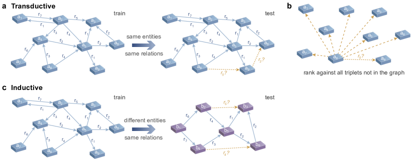
Figure 7: Illustration of task details. (a) Depiction of the transductive knowledge graph completion process. (b) Illustration of the filtered ranking protocol used to rank the test triplet $(x,q,y)$ against all negative triplets absent from the graph. The triplets $(x^{\prime},q,y)$ are not shown here for clarity. (c) Illustration of the inductive setting of relation prediction.

We illustrate the tasks of transductive knowledge graph completion and inductive relation prediction in Fig. 7. For homogeneous graph link prediction, it is similar to transductive knowledge graph completion except that there is only one relation type in homogeneous graphs, i.e., the existence of the edge.

E.3 Experimental Details

Datasets and preprocessing

We assess our model across various tasks including transductive knowledge graph completion, inductive knowledge graph relation prediction, and homogeneous graph link prediction. For knowledge graphs, we employ the widely recognized FB15k-237 (Toutanova & Chen, 2015) and WN18RR (Dettmers et al., 2018), adhering to the standard transductive (Toutanova & Chen, 2015; Dettmers et al., 2018) and inductive splits (Teru et al., 2020). For homogeneous graphs, we utilize Cora, Citeseer, and PubMed (Sen et al., 2008).

In evaluating knowledge graph completion, we adhere to the prevalent filtered ranking protocol (Bordes et al., 2013), ranking a test triplet $(x,q,y)$ against all negative triplets $(x,q,y^{\prime})$ or $(x^{\prime},q,y)$ absent in the graph (considering the likelihood score). We report MR, MRR, and HITS at N. For inductive knowledge graph relation prediction, we align with the previous practice (Teru et al., 2020), drawing 50 negative triplets for each positive one using the aforementioned filtered ranking and report HITS@10. In the context of homogeneous graph link prediction, we follow the approaches of Kipf & Welling (2016), contrasting the positive edges with an equivalent number of negative edges, and report AUROC and AP. The distribution of edges in train/valid/test is maintained at a ratio of 85:5:10, aligning with common practice. The specifics and statistics related to the datasets are available in Appendix D.

Regarding data preprocessing, we adhere to the methodologies of prior works (Yang et al., 2017; Sadeghian et al., 2019; Kipf & Welling, 2016). In knowledge graphs, each triplet $(x,q,y)$ is augmented with a reversed triplet $(y,q^{-1},x)$. In homogeneous graphs, each node is augmented with a self-loop. Additionally, we follow Zhu et al. (2021) to exclude edges directly connecting query node pairs during the training phase for the transductive setting of FB15k-237 and homogeneous graphs.

Models and training

Given the substantial computational expense associated with simulating SNNs over a long time, our primary simulations involve $T=10$ discrete time steps for SNNs. The hyperparameters for SNNs are designated as $\tau_{m}/\Delta\tau=4,V_{th}=2$, with the discrete delay bound $\beta=4$, and $\lambda=0.95$ for the decoding function. This can correspond to $\tau_{m}=\tau_{c}=20ms$ with discretization interval $\Delta\tau=5ms$ and a total simulation time $T\times\Delta\tau=50ms$ for SNNs. For experiments analyzing temporal discretization steps in Section F.3, hyperparameters are adjusted relative to the discrete step; for instance, for $T=5$, we assign $\tau_{m}/\Delta\tau=2,\beta=2,\lambda=0.9$ (corresponding to $\Delta\tau=10ms$), and for $T=20$, we designate $\tau_{m}/\Delta\tau=8,\beta=8,\lambda=0.97$ (corresponding to $\Delta\tau=2.5ms$). Each graph node is represented by $n=32$ spiking neurons by default. No normalization or other modifications are applied, and for models on FB15k-237, a linear scale of $0.1$ is applied post the linear transformation $\mathbf{W}$.

As for the two baseline SNN models that we compare in Section 4 to elucidate the superiority of synaptic delay, the first model abstains from encoding edge relations, and the delay $\mathbf{d}_{r}^{q}$ in Eq. 7 is not taken into account, i.e., it is assigned a value of zero. The second model opts for encoding relations through synaptic weight instead of synaptic delay. We modify $\mathbf{s}^{q}_{k}[t-\mathbf{d}^{q}_{r}]$ in Eq. 7 to $\mathbf{w}_{r}^{q}\odot\mathbf{s}^{q}_{k}[t]$ (where $\mathbf{w}_{r}^{q}$ is defined analogously to $\mathbf{d}^{q}_{r}$ but devoid of the sigmoid function and bound scale, and $\mathbf{w}_{r}^{q}$ can be amalgamated into $\mathbf{W}$ to formulate the entire synaptic weight). This alteration aligns with the DistMult message function utilized in prior works to multiply messages with edge representations (Zhu et al., 2021).

For GRSNN+, we apply layer normalization (LN) after the linear transformation of the aggregated messages as in many GNNs, and encode relations in both synaptic delay and synaptic weight, i.e., the messages are $\mathbf{w}_{r}^{q}\odot\mathbf{s}^{q}_{k}[t-\mathbf{d}^{q}_{r}]$. For FB15k-237, we further adopt the principal neighborhood aggregation (PNA) as the aggregation function instead of summation, which is a major component for the high performance of NBFNet (Zhu et al., 2021). We show that by integrating these GNN tricks, GRSNN can also achieve a better performance.

All models are trained utilizing the Adam optimizer over 20 epochs. The learning rate is $2e-3$ for transductive settings (knowledge graph completion and homogeneous graph link prediction) and $5e-3$ for inductive settings. The batch size is 32 (30 for transductive FB15k-237), achieved by accumulating gradients across several iterations with smaller mini-batches each iteration.

The ratio of negative samples is configured to 256 for FB15k-237 and WN18RR in the transductive setting and 50 in the inductive setting to align more closely with testing conditions, while it is established as $1$ for homogeneous graphs, adhering to previous studies. The temperature in self-adversarial negative sampling is determined to be 0.5 and 1 for FB15k-237 and WN18RR, respectively. Model selection is based on validation performance, with MRR serving as the criterion for knowledge graphs and AUROC for homogeneous graphs.

Our code implementation leverages the PyTorch framework, and experimental evaluations are executed on one or two NVIDIA GeForce RTX 3090 GPUs.

Details of theoretical energy estimation

For theoretical inference operation counts and energy estimations, we consider the scenario where neural network models are deployed and mapped directly to individual neurons and synapses. This scenario aligns with the principles of neuromorphic computing and hardware (Davies et al., 2018; Pei et al., 2019; Rao et al., 2022), facilitating in-memory computation and minimizing energy-consuming memory exchanges. Our theoretical analysis predominantly centers on the operations of neurons and synapses, omitting additional hardware-related costs such as memory access.

For the spiking model, the estimated synaptic operations are given by $T\times n^{2}\times fr\times|\mathcal{E}|$, where $T$ represents the discrete time step, $n$ is the number of neurons allocated per graph node, $fr$ denotes the spike rate, and $|\mathcal{E}|$ is the count of graph edges. This calculation corresponds to the quantity of synaptic operations instigated by spikes, culminating in an accumulation (addition) operation of post-synaptic current (or membrane potential). Additionally, accounting for neuron dynamics, there will be $T\times n\times|\mathcal{V}|$ addition operations for the bias term, $T\times n\times|\mathcal{V}|$ addition operations for the accumulation of membrane potential with current, and $2T\times n\times|\mathcal{V}|$ multiplication operations due to the leakage of current and membrane potential, where $|\mathcal{V}|$ represents the number of graph nodes. The computational cost associated with spike generation and reset is omitted in this estimation. Consequently, the total operations involve $2T\times n\times|\mathcal{V}|$ multiplications and $T\times n^{2}\times fr\times|\mathcal{E}|+2T\times n\times|\mathcal{V}|$ additions.

For the non-spiking counterpart, assuming the replacement of spiking neurons with conventional artificial neurons and disregarding the computational cost of the activation function, the synaptic operations would involve $T\times n^{2}\times|\mathcal{E}|$ MAC operations (multiplication + addition), along with $T\times n\times|\mathcal{V}|$ addition operations for the bias term. Thus, the total operations would encompass $T\times n^{2}\times|\mathcal{E}|$ multiplications and $T\times n^{2}\times(|\mathcal{E}|+|\mathcal{V}|)$ additions.

Costs of synaptic delay

We consider the Ring Buffer for potential synaptic delay implementation as analyzed in Patiño-Saucedo et al. (2023), which is commonly used by digital neuromorphic platforms. The memory overhead of the ring buffer is the number of neurons multiplied by the maximum synaptic delay $M_{d}$, and the energy overhead is equal to one extra neural accumulation per time step for each neuron (Patiño-Saucedo et al., 2023). Then, the additional memory overhead (words) is $n\times|\mathcal{V}|\times M_{d}$ and the additional energy overhead is $T\times n\times|\mathcal{V}|\times E_{AC}$. Consider the original memory overhead $n\times|\mathcal{V}|\times 2+n^{2}\times|\mathcal{E}|$ (neuron states + synapses) and the original energy overhead $2T\times n\times|\mathcal{V}|\times E_{MAC}+(T\times n^{2}\times fr\times|\mathcal{E}|+2T\times n\times|\mathcal{V}|)\times E_{AC}$ (analyzed above), the additional overhead is small because the number of synapses is much larger than the number of neurons ($n^{2}\times|\mathcal{E}|\gg n\times|\mathcal{V}|$) in our settings. Specifically, on the test set of FB15k-237, the originally analyzed energy is estimated as 1.337 mJ, while the additional energy for synaptic delay is estimated as 0.004 mJ, which is marginal.

Visualization of reasoning paths

The methodology for visualizing reasoning paths in Section F.2 is elucidated below. The interpretation of reasoning is predicated on the significance of paths to the concluding prediction score. According to Zhu et al. (2021), this significance or importance can be computed by the gradient of the prediction with respect to the paths, based on the local 1st-order Taylor expansion, and the path importance can be approximated by summing the importance of the edges in the path. This edge importance is computed using automatic differentiation. Specifically, during the forward procedure, the variable of edge weight (initialized to 1) is multiplied to the message transmitted through this edge (i.e., the delayed spikes, with 1 representing a spike and 0 representing no spike). Only when a spike is present will there be a gradient for this variable during backpropagation. Subsequently, during backpropagation, this variable accumulates the gradients of all neurons at every time step, representing the edge importance.

For the non-differentiable spiking operation, a distinct surrogate gradient is employed for backpropagation. If the membrane potential $u$ is below the threshold, the gradient is set to 0, as there is no output spike influencing other neurons. Conversely, if the membrane potential surpasses the threshold, the gradient is set as $1/u$, normalizing the contribution of inputs to the output based on the membrane potential, as the gradient of the output is for spike $1$.

The top-k path importance is thus analogous to the top-k longest paths when considering edge importance. We adopt a beam search, as suggested by Zhu et al. (2021), to identify these paths. It is crucial to note that this method provides only a rough approximation, and future research may explore more refined interpretative approaches.

Appendix F More Results and Detailed Values

F.1 Detailed Values of Main Results

In this section, we furnish detailed results for various experiments. The comprehensive result values for transductive knowledge graph completion are presented in Table 6. For inductive relation prediction, the detailed results can be referred to in Table 7. Lastly, the exhaustive result values for homogeneous graph link prediction are available in Table 8.

Table 6: Detailed Results for Transductive Knowledge Graph Completion. Lower values are preferable for MR, while higher values are preferable for MRR, HITS@1, HITS@3, and HITS@10. *SpikTE is an embedding method based on spiking neurons.

(b)
Class	Method	FB15k-237					WN18RR
		MR$\downarrow$	MRR$\uparrow$	H@1$\uparrow$	H@3$\uparrow$	H@10$\uparrow$	MR$\downarrow$	MRR$\uparrow$	H@1$\uparrow$	H@3$\uparrow$	H@10$\uparrow$
Path-based	Path Ranking (Lao & Cohen, 2010)	3521	0.174	0.119	0.186	0.285	22438	0.324	0.276	0.360	0.406
	NeuralLP (Yang et al., 2017)	-	0.240	-	-	0.362	-	0.435	0.371	0.434	0.566
	DRUM (Sadeghian et al., 2019)	-	0.343	0.255	0.378	0.516	-	0.486	0.425	0.513	0.586
Embeddings	TransE (Bordes et al., 2013)	357	0.294	-	-	0.465	3384	0.226	-	-	0.501
	DistMult (Yang et al., 2015)	254	0.241	0.155	0.263	0.419	5110	0.43	0.39	0.44	0.49
	ComplEx (Trouillon et al., 2016)	339	0.247	0.158	0.275	0.428	5261	0.44	0.41	0.46	0.51
	RotatE (Sun et al., 2019)	177	0.338	0.241	0.375	0.533	3340	0.476	0.428	0.492	0.571
	LowFER (Amin et al., 2020)	-	0.359	0.266	0.396	0.544	-	0.465	0.434	0.479	0.526
	SpikTE* (Dold, 2022)	-	0.21	0.13	0.23	-	-	-	-	-	-
GNNs	RGCN (Schlichtkrull et al., 2018)	221	0.273	0.182	0.303	0.456	2719	0.402	0.345	0.437	0.494
	GraIL (Teru et al., 2020)	2053	-	-	-	-	2539	-	-	-	-
	CompGCN (Vashishth et al., 2020)	197	0.355	0.264	0.390	0.535	3533	0.479	0.443	0.494	0.546
	NBFNet (Zhu et al., 2021)	114	0.415	0.321	0.454	0.599	636	0.551	0.497	0.573	0.666
SNNs	GRSNN (ours)	139	0.368	0.275	0.407	0.551	720	0.508	0.455	0.528	0.616
	GRSNN+ (ours)	132	0.393	0.301	0.431	0.572	610	0.532	0.478	0.557	0.637

Table 7: Detailed Results for Inductive Relation Prediction (HITS@10). v1-v4 correspond to the four standard versions of inductive splits.

Class	Method	FB15k-237				WN18RR
		v1	v2	v3	v4	v1	v2	v3	v4
Path-based	NeuralLP (Yang et al., 2017)	0.529	0.589	0.529	0.559	0.744	0.689	0.462	0.671
	DRUM (Sadeghian et al., 2019)	0.529	0.587	0.529	0.559	0.744	0.689	0.462	0.671
	RuleN (Meilicke et al., 2018)	0.498	0.778	0.877	0.856	0.809	0.782	0.534	0.716
GNNs	GraIL (Teru et al., 2020)	0.642	0.818	0.828	0.893	0.825	0.787	0.584	0.734
	NBFNet (Zhu et al., 2021)	0.834	0.949	0.951	0.960	0.948	0.905	0.893	0.890
SNNs	GRSNN (ours)	0.852	0.957	0.958	0.958	0.943	0.892	0.906	0.888

Table 8: Detailed Results for Homogeneous Graph Link Prediction.

Class	Method	Cora		Citeseer		PubMed
		AUROC$\uparrow$	AP$\uparrow$	AUROC$\uparrow$	AP$\uparrow$	AUROC$\uparrow$	AP$\uparrow$
Path-based	Katz Index (Katz, 1953)	0.834	0.889	0.768	0.810	0.757	0.856
	Personalized PageRank (Page et al., 1999)	0.845	0.899	0.762	0.814	0.763	0.860
Embeddings	DeepWalk (Perozzi et al., 2014)	0.831	0.850	0.805	0.836	0.844	0.841
	LINE (Tang et al., 2015)	0.844	0.876	0.791	0.826	0.849	0.888
	node2vec (Grover & Leskovec, 2016)	0.872	0.879	0.838	0.868	0.891	0.914
GNNs	VGAE (Kipf & Welling, 2016)	0.914	0.926	0.908	0.920	0.944	0.947
	S-VGAE (Davidson et al., 2018)	0.941	0.941	0.947	0.952	0.960	0.960
	SEAL (Zhang & Chen, 2018)	0.933	0.942	0.905	0.924	0.978	0.979
	TLC-GNN (Yan et al., 2021)	0.934	0.931	0.909	0.916	0.970	0.968
	NBFNet (Zhu et al., 2021)	0.956	0.962	0.923	0.936	0.983	0.982
SNNs	GRSNN (ours)	0.936	0.945	0.915	0.931	0.982	0.982

F.2 Interpretability

The visualization of the reasoning paths for the final predictions of several examples are shown in Table 9. It is calculated based on edge and path importance (refer to Section E.3). As shown in the results, GRSNN is adept at discerning relation relevances and exploiting transitions, for instance, “contains”, and analogs, such as individuals with analogous “award”.

Table 9: Visualization of the top-2 reasoning paths for examples on FB15k237. It is determined by path importances derived from edge importances. The superscript ^-1 indicates the inverse relation.

Query	$(x,q,y):$ (england, contains, pontefract)
0.967	(england, contains, west yorkshire) $\land$ (west yorkshire, contains, pontefract)
0.671	(england, contains, leodis) $\land$ (leodis, contains-1, west yorkshire) $\land$ (west yorkshire, contains, pontefract)
Query	$(x,q,y):$ (58th academy awards nominees and winners, honored for, kiss of the spider woman (film))
1.482	(58th academy awards nominees and winners, award winner, William Hurt)
	$\land$ (William Hurt, film, kiss of the spider woman (film))
1.347	(58th academy awards nominees and winners, award winner, William Hurt)
	$\land$ (William Hurt, nominated for, kiss of the spider woman (film))
Query	$(x,q,y):$ (florida (rapper), profession, artiste)
0.513	(florida (rapper), award, grammy award for album of the year 2010s)
	$\land$ (grammy award for album of the year 2010s, award-1, kanye west) $\land$ (kanye west, profession, artiste)
0.512	(florida (rapper), award, grammy award for album of the year 2010s)
	$\land$ (grammy award for album of the year 2010s, award-1, witney houston) $\land$ (witney houston, profession, artiste)

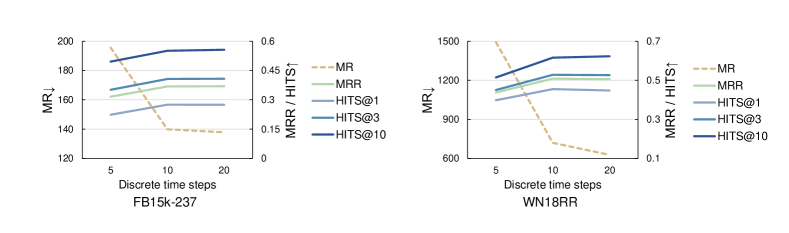
Figure 8: Analysis of the temporal discretization of GRSNN under varying discrete time steps.

F.3 Impact of Discretization Steps

The impact of temporal discretization with different intervals and steps on GRSNN is explored in Fig. 8, and the details of hyperparameters are explained in Section E.3. Given the substantial computational cost associated with simulating SNNs over extended periods, experiments primarily employ $T=10$ discrete time steps for GRSNN. The results indicate that a reduced number of time steps (5) with a larger discretization interval significantly impairs performance due to discretization error, while a larger setting (20) with a smaller interval offers marginal improvements, maintaining comparable results to 10 time steps. This demonstrates the model’s robustness under relatively low latency with minimal discrete time steps.

Table 10: Analysis results of GRSNN with varying neuron number per graph node on WN18RR.

Neuron number per node	Parameters	MR$\downarrow$	MRR$\uparrow$	H@1$\uparrow$	H@3$\uparrow$	H@10$\uparrow$
8	1.9K	967	0.452	0.405	0.464	0.551
16	6.9K	819	0.483	0.430	0.500	0.597
32	26K	720	0.508	0.455	0.528	0.616
64	101K	668	0.522	0.469	0.544	0.632
96	226K	648	0.523	0.470	0.546	0.630

Table 11: Comparison results of different final MLP types on WN18RR.

Final MLP type	MR$\downarrow$	MRR$\uparrow$	H@1$\uparrow$	H@3$\uparrow$	H@10$\uparrow$
ReLU	720	0.508	0.455	0.528	0.616
spiking	701	0.502	0.447	0.521	0.615

Table 12: Error bar on WN18RR.

MR$\downarrow$	MRR$\uparrow$	H@1$\uparrow$	H@3$\uparrow$	H@10$\uparrow$
707$\pm$22	0.508$\pm$0.000	0.455$\pm$0.001	0.528$\pm$0.000	0.616$\pm$0.001

F.4 Impact of Neuron Number and Parameter Amount

As described in Section E.3, we take $n=32$ spiking neurons for each graph node, which is consistent with many previous graph neural network works (Zhu et al., 2021). To further study the impact of neuron number as well as the corresponding parameter amount, we explore results with varying neuron numbers per node in this section. As shown in Table 10, the performance will grow as parameters increase and 32 neurons per node are not optimal. On the other hand, more neurons lead to a larger computational complexity, and there exists a trade-off between performance and complexity.

F.5 Spiking Link Prediction Head

As explained in Section E.1, we leverage a feedforward neural network $g$ to estimate the conditional likelihood of the given pair representation $\mathbf{h}^{q}(x,y)$, and following previous work (Zhu et al., 2021), $g$ is implemented as a two-layer MLP with ReLU activation. While this network can be converted to a spiking MLP through rate or temporal coding (Rueckauer et al., 2017; Stöckl & Maass, 2021) to enable a fully spiking system, we further study if we can directly and jointly train a spiking network for this link prediction head. To this end, we replace the ReLU activation with a simple non-leaky Integrate and Fire neuron model combined with the simple current model (i.e., the input current is the linear combination with spikes without dynamics, $I_{i}(t)=\sum_{j}w_{ij}s_{j}(t)+b_{i}$), consider rate coding over four discrete time steps, and use surrogate derivatives for training. As shown in Table 11, the performance of spiking MLP is almost the same as that with ReLU activation because the major component of the task is to extract pair representations, which is done by the main GRSNN part.

F.6 Error Bar

We investigate the error bar of our method on WN18RR based on three runs of experiments with different random seeds. Table 12 shows that the variance of different runs is extremely small, indicating the robustness of the method.

Appendix G More Discussions

Knowledge reasoning in human brains involves many neurophysiological processes across many brain areas, and how this is implemented is not fully understood. In this work, we mainly focus on neuro-inspired methods in AI task formulation to investigate how SNNs as computational models can deal with (knowledge) graph reasoning, while it can be future work to study better correspondence with neuroscience.

For neuromorphic hardware, on-chip memory limitation is an issue, so it may not directly support large-scale graphs. But neuromorphic hardware is rapidly developing for larger memories, for example, Intel’s Loihi 2 can support 1 million neurons and 120 million synapses. While this may still not fully support 32 neurons per node for some knowledge graphs, but fewer neurons, such as 16, could be acceptable, and it works for our method with some trade-off for performance (as shown in Section F.4). As neuromorphic computing is a rapidly developing field considering both hardware and algorithm, this paper do not restrict algorithms to some existing hardware, but focuses on the algorithm level with theoretical analysis considering hardware (energy), aligning with previous SNNs works. Actually, algorithms can potentially guide future software-hardware co-design (Schuman et al., 2022). We hope this work could serve as a catalyst for deeper insights and wider applications of neuromorphic computing systems.

References

- Aimone et al. (2021) Aimone, J. B., Ho, Y., Parekh, O., Phillips, C. A., Pinar, A., Severa, W., and Wang, Y. Provable advantages for graph algorithms in spiking neural networks. In ACM Symposium on Parallelism in Algorithms and Architectures (SPAA), 2021.
- Amin et al. (2020) Amin, S., Varanasi, S., Dunfield, K. A., and Neumann, G. Lowfer: Low-rank bilinear pooling for link prediction. In International Conference on Machine Learning (ICML), 2020.
- Bellec et al. (2018) Bellec, G., Salaj, D., Subramoney, A., Legenstein, R., and Maass, W. Long short-term memory and learning-to-learn in networks of spiking neurons. In Advances in Neural Information Processing Systems (NeurIPS), 2018.
- Bellec et al. (2020) Bellec, G., Scherr, F., Subramoney, A., Hajek, E., Salaj, D., Legenstein, R., and Maass, W. A solution to the learning dilemma for recurrent networks of spiking neurons. Nature Communications, 11(1):1–15, 2020.
- Bordes et al. (2013) Bordes, A., Usunier, N., Garcia-Duran, A., Weston, J., and Yakhnenko, O. Translating embeddings for modeling multi-relational data. In Advances in Neural Information Processing Systems (NeurIPS), 2013.
- Chakraborty & Mukhopadhyay (2023) Chakraborty, B. and Mukhopadhyay, S. Heterogeneous neuronal and synaptic dynamics for spike-efficient unsupervised learning: Theory and design principles. In International Conference on Learning Representations (ICLR), 2023.
- Comsa et al. (2020) Comsa, I. M., Potempa, K., Versari, L., Fischbacher, T., Gesmundo, A., and Alakuijala, J. Temporal coding in spiking neural networks with alpha synaptic function. In IEEE International Conference on Acoustics, Speech and Signal Processing (ICASSP), 2020.
- Davidson et al. (2018) Davidson, T. R., Falorsi, L., De Cao, N., Kipf, T., and Tomczak, J. M. Hyperspherical variational auto-encoders. In Conference on Uncertainty in Artificial Intelligence (UAI), 2018.
- Davies et al. (2018) Davies, M., Srinivasa, N., Lin, T.-H., Chinya, G., Cao, Y., Choday, S. H., Dimou, G., Joshi, P., Imam, N., Jain, S., et al. Loihi: A neuromorphic manycore processor with on-chip learning. IEEE Micro, 38(1):82–99, 2018.
- Dettmers et al. (2018) Dettmers, T., Minervini, P., Stenetorp, P., and Riedel, S. Convolutional 2d knowledge graph embeddings. In AAAI Conference on Artificial Intelligence (AAAI), 2018.
- Dold (2022) Dold, D. Relational representation learning with spike trains. In International Joint Conference on Neural Networks (IJCNN), 2022.
- Dold & Garrido (2021) Dold, D. and Garrido, J. S. Spike: Spike-based embeddings for multi-relational graph data. In International Joint Conference on Neural Networks (IJCNN), 2021.
- Fang et al. (2022) Fang, H., Zeng, Y., Tang, J., Wang, Y., Liang, Y., and Liu, X. Brain-inspired graph spiking neural networks for commonsense knowledge representation and reasoning. arXiv preprint arXiv:2207.05561, 2022.
- Fang et al. (2021) Fang, W., Yu, Z., Chen, Y., Masquelier, T., Huang, T., and Tian, Y. Incorporating learnable membrane time constant to enhance learning of spiking neural networks. In International Conference on Computer Vision (ICCV), 2021.
- Grover & Leskovec (2016) Grover, A. and Leskovec, J. node2vec: Scalable feature learning for networks. In ACM SIGKDD International Conference on Knowledge Discovery and Data Mining (KDD), 2016.
- Hammouamri et al. (2024) Hammouamri, I., Khalfaoui-Hassani, I., and Masquelier, T. Learning delays in spiking neural networks using dilated convolutions with learnable spacings. In International Conference on Learning Representations (ICLR), 2024.
- Horowitz (2014) Horowitz, M. 1.1 computing’s energy problem (and what we can do about it). In IEEE International Solid-State Circuits Conference (ISSCC), 2014.
- Huxter et al. (2003) Huxter, J., Burgess, N., and O’Keefe, J. Independent rate and temporal coding in hippocampal pyramidal cells. Nature, 425(6960):828–832, 2003.
- Katz (1953) Katz, L. A new status index derived from sociometric analysis. Psychometrika, 18(1):39–43, 1953.
- Kemp & Tenenbaum (2008) Kemp, C. and Tenenbaum, J. B. The discovery of structural form. Proceedings of the National Academy of Sciences (PNAS), 105(31):10687–10692, 2008.
- Kipf & Welling (2016) Kipf, T. N. and Welling, M. Variational graph auto-encoders. arXiv preprint arXiv:1611.07308, 2016.
- Lao & Cohen (2010) Lao, N. and Cohen, W. W. Relational retrieval using a combination of path-constrained random walks. Machine Learning, 81:53–67, 2010.
- Li et al. (2023) Li, J., Yu, Z., Zhu, Z., Chen, L., Yu, Q., Zheng, Z., Tian, S., Wu, R., and Meng, C. Scaling up dynamic graph representation learning via spiking neural networks. In AAAI Conference on Artificial Intelligence (AAAI), 2023.
- Li et al. (2021) Li, Y., Deng, S., Dong, X., Gong, R., and Gu, S. A free lunch from ann: Towards efficient, accurate spiking neural networks calibration. In International Conference on Machine Learning (ICML), 2021.
- Liben-Nowell & Kleinberg (2007) Liben-Nowell, D. and Kleinberg, J. The link-prediction problem for social networks. Journal of the American Society for Information Science and Technology, 58(7):1019–1031, 2007.
- Lv et al. (2023) Lv, C., Xu, J., and Zheng, X. Spiking convolutional neural networks for text classification. In International Conference on Learning Representations (ICLR), 2023.
- Maass (1997) Maass, W. Networks of spiking neurons: the third generation of neural network models. Neural Networks, 10(9):1659–1671, 1997.
- Meilicke et al. (2018) Meilicke, C., Fink, M., Wang, Y., Ruffinelli, D., Gemulla, R., and Stuckenschmidt, H. Fine-grained evaluation of rule-and embedding-based systems for knowledge graph completion. In International Semantic Web Conference (ISWC), 2018.
- Meng et al. (2022a) Meng, Q., Xiao, M., Yan, S., Wang, Y., Lin, Z., and Luo, Z.-Q. Training high-performance low-latency spiking neural networks by differentiation on spike representation. In Conference on Computer Vision and Pattern Recognition (CVPR), 2022a.
- Meng et al. (2022b) Meng, Q., Yan, S., Xiao, M., Wang, Y., Lin, Z., and Luo, Z.-Q. Training much deeper spiking neural networks with a small number of time-steps. Neural Networks, 153:254–268, 2022b.
- Mostafa (2017) Mostafa, H. Supervised learning based on temporal coding in spiking neural networks. IEEE Transactions on Neural Networks and Learning Systems (TNNLS), 29(7):3227–3235, 2017.
- Nickel et al. (2015) Nickel, M., Murphy, K., Tresp, V., and Gabrilovich, E. A review of relational machine learning for knowledge graphs. Proceedings of the IEEE, 104(1):11–33, 2015.
- Page et al. (1999) Page, L., Brin, S., Motwani, R., and Winograd, T. The pagerank citation ranking: Bringing order to the web. Technical report, Stanford InforLab, 1999.
- Patiño-Saucedo et al. (2023) Patiño-Saucedo, A., Yousefzadeh, A., Tang, G., Corradi, F., Linares-Barranco, B., and Sifalakis, M. Empirical study on the efficiency of spiking neural networks with axonal delays, and algorithm-hardware benchmarking. In IEEE International Symposium on Circuits and Systems (ISCAS). IEEE, 2023.
- Pei et al. (2019) Pei, J., Deng, L., Song, S., Zhao, M., Zhang, Y., Wu, S., Wang, G., Zou, Z., Wu, Z., He, W., et al. Towards artificial general intelligence with hybrid Tianjic chip architecture. Nature, 572(7767):106–111, 2019.
- Perozzi et al. (2014) Perozzi, B., Al-Rfou, R., and Skiena, S. Deepwalk: Online learning of social representations. In ACM SIGKDD International Conference on Knowledge Discovery and Data Mining (KDD), 2014.
- Rao et al. (2022) Rao, A., Plank, P., Wild, A., and Maass, W. A long short-term memory for AI applications in spike-based neuromorphic hardware. Nature Machine Intelligence, 4(5):467–479, 2022.
- Reinagel & Reid (2000) Reinagel, P. and Reid, R. C. Temporal coding of visual information in the thalamus. Journal of Neuroscience, 20(14):5392–5400, 2000.
- Roy et al. (2019) Roy, K., Jaiswal, A., and Panda, P. Towards spike-based machine intelligence with neuromorphic computing. Nature, 575(7784):607–617, 2019.
- Rueckauer et al. (2017) Rueckauer, B., Lungu, I.-A., Hu, Y., Pfeiffer, M., and Liu, S.-C. Conversion of continuous-valued deep networks to efficient event-driven networks for image classification. Frontiers in Neuroscience, 11:682, 2017.
- Sadeghian et al. (2019) Sadeghian, A., Armandpour, M., Ding, P., and Wang, D. Z. Drum: End-to-end differentiable rule mining on knowledge graphs. In Advances in Neural Information Processing Systems (NeurIPS), 2019.
- Santoro et al. (2017) Santoro, A., Raposo, D., Barrett, D. G., Malinowski, M., Pascanu, R., Battaglia, P., and Lillicrap, T. A simple neural network module for relational reasoning. In Advances in Neural Information Processing Systems (NeurIPS), 2017.
- Schlichtkrull et al. (2018) Schlichtkrull, M., Kipf, T. N., Bloem, P., Van Den Berg, R., Titov, I., and Welling, M. Modeling relational data with graph convolutional networks. In European Semantic Web Conference (ESWC), 2018.
- Schuman et al. (2022) Schuman, C. D., Kulkarni, S. R., Parsa, M., Mitchell, J. P., Kay, B., et al. Opportunities for neuromorphic computing algorithms and applications. Nature Computational Science, 2(1):10–19, 2022.
- Sen et al. (2008) Sen, P., Namata, G., Bilgic, M., Getoor, L., Galligher, B., and Eliassi-Rad, T. Collective classification in network data. AI Magazine, 29(3):93–93, 2008.
- Shrestha & Orchard (2018) Shrestha, S. B. and Orchard, G. Slayer: spike layer error reassignment in time. In Advances in Neural Information Processing Systems (NeurIPS), 2018.
- Stöckl & Maass (2021) Stöckl, C. and Maass, W. Optimized spiking neurons can classify images with high accuracy through temporal coding with two spikes. Nature Machine Intelligence, 3(3):230–238, 2021.
- Sun et al. (2019) Sun, Z., Deng, Z.-H., Nie, J.-Y., and Tang, J. Rotate: Knowledge graph embedding by relational rotation in complex space. In International Conference on Learning Representations (ICLR), 2019.
- Tang et al. (2015) Tang, J., Qu, M., Wang, M., Zhang, M., Yan, J., and Mei, Q. Line: Large-scale information network embedding. In International Conference on World Wide Web (WWW), 2015.
- Teru et al. (2020) Teru, K., Denis, E., and Hamilton, W. Inductive relation prediction by subgraph reasoning. In International Conference on Machine Learning (ICML), 2020.
- Toutanova & Chen (2015) Toutanova, K. and Chen, D. Observed versus latent features for knowledge base and text inference. In Proceedings of the 3rd Workshop on Continuous Vector Space Models and their Compositionality, 2015.
- Trouillon et al. (2016) Trouillon, T., Welbl, J., Riedel, S., Gaussier, É., and Bouchard, G. Complex embeddings for simple link prediction. In International Conference on Machine Learning (ICML), 2016.
- Vashishth et al. (2020) Vashishth, S., Sanyal, S., Nitin, V., and Talukdar, P. Composition-based multi-relational graph convolutional networks. In International Conference on Learning Representations (ICLR), 2020.
- Wang et al. (2023) Wang, H., Fu, T., Du, Y., Gao, W., Huang, K., Liu, Z., Chandak, P., Liu, S., Van Katwyk, P., Deac, A., et al. Scientific discovery in the age of artificial intelligence. Nature, 620(7972):47–60, 2023.
- Xiao et al. (2021) Xiao, M., Meng, Q., Zhang, Z., Wang, Y., and Lin, Z. Training feedback spiking neural networks by implicit differentiation on the equilibrium state. In Advances in Neural Information Processing Systems (NeurIPS), 2021.
- Xiao et al. (2022) Xiao, M., Meng, Q., Zhang, Z., He, D., and Lin, Z. Online training through time for spiking neural networks. In Advances in Neural Information Processing Systems (NeurIPS), 2022.
- Xiao et al. (2024) Xiao, M., Meng, Q., Zhang, Z., He, D., and Lin, Z. Hebbian learning based orthogonal projection for continual learning of spiking neural networks. In International Conference on Learning Representations (ICLR), 2024.
- Yan et al. (2024) Yan, S., Meng, Q., Xiao, M., Wang, Y., and Lin, Z. Sampling complex topology structures for spiking neural networks. Neural Networks, 172:106121, 2024.
- Yan et al. (2021) Yan, Z., Ma, T., Gao, L., Tang, Z., and Chen, C. Link prediction with persistent homology: An interactive view. In International Conference on Machine Learning (ICML), 2021.
- Yang et al. (2015) Yang, B., Yih, S. W.-t., He, X., Gao, J., and Deng, L. Embedding entities and relations for learning and inference in knowledge bases. In International Conference on Learning Representations (ICLR), 2015.
- Yang et al. (2017) Yang, F., Yang, Z., and Cohen, W. W. Differentiable learning of logical rules for knowledge base reasoning. In Advances in Neural Information Processing Systems (NeurIPS), 2017.
- Yin et al. (2021) Yin, B., Corradi, F., and Bohté, S. M. Accurate and efficient time-domain classification with adaptive spiking recurrent neural networks. Nature Machine Intelligence, 3(10):905–913, 2021.
- Zhang & Chen (2018) Zhang, M. and Chen, Y. Link prediction based on graph neural networks. In Advances in Neural Information Processing Systems (NeurIPS), 2018.
- Zhang et al. (2024) Zhang, Z., Xiao, M., Ji, T., Jiang, Y., Lin, T., Zhou, X., and Lin, Z. Efficient and generalizable cross-patient epileptic seizure detection through a spiking neural network. Frontiers in Neuroscience, 17:1303564, 2024.
- Zheng et al. (2022) Zheng, H., Lin, H., Zhao, R., and Shi, L. Dance of snn and ann: Solving binding problem by combining spike timing and reconstructive attention. In Advances in Neural Information Processing Systems (NeurIPS), 2022.
- Zhou et al. (2021) Zhou, S., Li, X., Chen, Y., Chandrasekaran, S. T., and Sanyal, A. Temporal-coded deep spiking neural network with easy training and robust performance. In AAAI Conference on Artificial Intelligence (AAAI), 2021.
- Zhu et al. (2021) Zhu, Z., Zhang, Z., Xhonneux, L.-P., and Tang, J. Neural bellman-ford networks: A general graph neural network framework for link prediction. In Advances in Neural Information Processing Systems (NeurIPS), 2021.
- Zhu et al. (2022) Zhu, Z., Peng, J., Li, J., Chen, L., Yu, Q., and Luo, S. Spiking graph convolutional networks. In International Joint Conference on Artificial Intelligence (IJCAI), 2022.