UniCompress: Enhancing Multi-Data Medical Image Compression with Knowledge Distillation
Abstract
In the field of medical image compression, Implicit Neural Representation (INR) networks have shown remarkable versatility due to their flexible compression ratios, yet they are constrained by a one-to-one fitting approach that results in lengthy encoding times. Our novel method, “UniCompress”, innovatively extends the compression capabilities of INR by being the first to compress multiple medical data blocks using a single INR network. By employing wavelet transforms and quantization, we introduce a codebook containing frequency domain information as a prior input to the INR network. This enhances the representational power of INR and provides distinctive conditioning for different image blocks. Furthermore, our research introduces a new technique for the knowledge distillation of implicit representations, simplifying complex model knowledge into more manageable formats to improve compression ratios. Extensive testing on CT and electron microscopy (EM) datasets has demonstrated that UniCompress outperforms traditional INR methods and commercial compression solutions like HEVC, especially in complex and high compression scenarios. Notably, compared to existing INR techniques, UniCompress achieves a 45 times increase in compression speed, marking a significant advancement in the field of medical image compression. Codes will be publicly available.
1 Introduction
Implicit Neural Representations (INRs), which leverage neural networks to approximate continuous functions within complex data structures sitzmann2020implicit ; sitzmann2019scene ; zhang2021generator , were initially applied in scene rendering and reconstruction pumarola2021d ; martin2021nerf . Recent advancements have extended the use of INRs to lossy compression, achieving general, modality-agnostic compression by overfitting small networks yang2023sci ; yang2023tinc . INRs have demonstrated comparable performance to traditional methods in terms of objective metrics like PSNR and SSIM as well as image quality guo2023compression ; tang2024z ; tang2024zerothorder . However, in large-scale medical datasets, INR methods lag behind traditional methods yang2022sharing , primarily due to their local fitting approach, which often overlooks high-frequency information in images, resulting in excessive smoothing. Additionally, the one-to-one fitting approach of INRs leads to longer encoding times, posing significant challenges in large-scale medical image compression applications.
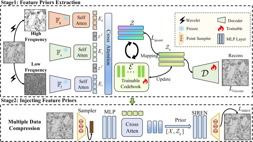
In this paper, we first theoretically analyze and compare the bounds on reconstruction errors for INR and VAE. We derive that if the INR decoder generates images closer to the original images with smaller magnitudes, INR will have a lower reconstruction error. Based on these insights, we introduce UniCompress, the first method capable of simultaneously compressing multiple data blocks, aiming to reduce encoding time and leverage existing knowledge. Our approach begins with a wavelet transform of medical image blocks, decomposing them into high-frequency and low-frequency components villasenor1995wavelet ; liu2018multi ; zhang2024deepgi . Robust visual features are then extracted using networks pretrained on large-scale medical images chen2023generative ; mo2024password ; pmlr-v216-tang23a . We employ an attention fusion module to integrate features from different modalities and use a learnable codebook esser2021taming to quantize the extracted multimodal features. This process combines discrete feature values with the numerical inputs of the INR, facilitating the parallel learning of multiple image block features and incorporating frequency domain information as priors.
To further enhance our method, we implement knowledge distillation wang2019private , where a smaller student network learns prior representations extracted by a larger teacher network. By aligning these representations through consistency in discrete codebook features and intermediate features in the reconstructed image space, we can significantly improve the compression ratio while maintaining visual quality.
Our comprehensive evaluation shows that using a simple MLP SIREN network, our method achieves an average PSNR improvement of 0.95 dB and 1.71 dB on CT and EM datasets, respectively, at the same compression ratio. Further distillation results yield performance gains of 0.71 dB and 0.77 dB. Moreover, we find that even cross-modal knowledge distillation aids performance, with out-of-domain knowledge providing more significant benefits in simpler datasets like Liver. Our method increases data encoding speed by 45 times, emphasizing efficient parallel processing across multiple datasets.
In summary, our contributions in this paper are as follows:
(1) We establish a theoretical analysis comparing the error bounds of INR and VAE, deriving sufficient conditions under which INR achieves lower reconstruction errors if the INR decoder generates images closer to the original with smaller magnitudes.
(2)We propose the first method that employs Implicit Neural Representations (INRs) to simultaneously represent multiple datasets. By incorporating a discrete codebook prior with frequency domain information, our network can represent diverse medical datasets concurrently.
(3) We introduce a two-stage training method using knowledge distillation, which transfers learned representations from complex models to simpler, smaller models, significantly enhancing inference speed and compression ratio.
(4) We conduct experiments on complex Electron Microscopy and CT data. Despite using only a basic SIREN scheme, our UniCompress demonstrates robust performance, validating its effectiveness in handling challenging datasets.
2 Related Work
Implicit Neural Representation. Recent advances in Implicit Neural Representations (INR) have shown significant progress. SIREN sitzmann2020implicit uses periodic activation functions for enhanced scene rendering. WIRE saragadam2023wire employs wavelet-based INR with complex Gabor wavelets for better visual signal representation and noise reduction. INCODE kazerouni2024incode integrates image priors for adaptive learning of activation function parameters.
In medical imaging, INRs like SIREN, ReLU, Snake, Sine+, and Chirp are effective for brain image registration by estimating displacement vectors and deformation fields byra2023exploring . For video frame interpolation (VFI), INRs align signal derivatives with optical flow to maintain brightness, outperforming some state-of-the-art models zhuang2022optical .
Medical Imaging Prior. Effective feature extraction enhances network performance. Zhou et al. zhou2023xnet used wavelet-transformed spectral features for segmentation, focusing on high-frequency areas. Chen et al. chen2023self used Histogram of Oriented Gradients (HOG) to balance performance and computational complexity. Self-supervised methods like multi-scale contrastive learning chen2023learning and text-image feature alignment chen2023generative ; chen2024bimcv have also shown progress.
Medical Image Compression. Efficient compression is crucial for large medical datasets. Traditional methods like JPEG 2000 and JP3D use wavelet transforms for optimal performance and complexity bruylants2015wavelet . Xue et al. xue2023dbvc achieve efficient 3D biomedical video encoding through motion estimation and compensation. Variational Autoencoders (VAEs) are also explored for lossy compression and structured MRI compression van2017neural . QARV duan2023qarv uses quantization-aware ResNet VAE, while Attri-VAE cetin2023attri provides attribute-based interpretable representations. INR-based methods like SCI yang2023sci and TINC yang2023tinc offer flexible block-wise approaches. COMBINER guo2023compression compresses data as INRs using relative entropy encoding. Despite their flexibility, INRs face challenges like low processing efficiency and high-frequency information loss. Our approach integrates medical image characteristics into INR inputs and processes multiple data blocks simultaneously, an unexplored area in INR compression for large-scale medical imaging.
INR-based methods like SCI yang2023sci and TINC yang2023tinc offer flexible block-wise approaches. COMBINER guo2023compression compresses data as INRs using relative entropy encoding. These methods are more flexible and universal across different modalities.
Despite their flexibility, INRs face challenges like low processing efficiency and high-frequency information loss. To address these, we integrate medical image characteristics into INR inputs through robust visual feature extraction and process multiple data blocks simultaneously. This approach is largely unexplored in INR compression for large-scale medical imaging.
3 Methodology
3.1 Problem Description
We tackle the problem of representing multiple volumetric medical images using a conditional INR network. Our objective is to encode a set of N volumetric medical images , where each represents a 3D image block, into a compressed format.
We begin by conducting a theoretical analysis to compare the bounds on reconstruction errors between INR and Variational Autoencoder (VAE) methods. Our analysis reveals that if the INR decoder generates images that are closer to the original images with smaller magnitudes, then the INR will have a lower reconstruction error (See in Section A). Based on this insight, we propose introducing prior frequency information into the INR framework.
The process begins with a specialized network, denoted as , which is designed to extract prior features from each image block . These prior features encapsulate essential structural and intensity characteristics of the volumetric data.
Given a set of spatial coordinates , the INR network is trained to predict the intensity value at , utilizing both the coordinates and the extracted prior features. The mapping function of the INR network is described as
| (1) |
where represents the predicted intensity value at coordinate , are the prior features corresponding to , and denotes the parameters of the INR network.
The compression ratio is determined by considering both the dimensions of the network parameters and the dimensions of the prior features . The aim is to optimize the INR network such that the reconstruction error between the original images and their reconstructions from the compressed representation is minimized, while also maximizing the compression ratio. The framework is shown in Figure 1.
3.2 Feature Quantization and Extraction
Our method combines wavelet transformation, pre-trained feature extraction, and codebook-based quantization to efficiently represent and reconstruct 3D medical images. The key steps are as follows:
Wavelet Transformation. We apply wavelet transformation to 3D medical images, extracting high-frequency, low-frequency, and original image features separately. The transformation is represented as
| (2) | ||||
where represents high-frequency information, represents low-frequency information, and are high-pass and low-pass wavelet functions.
To obtain high-dimensional 3D features, we employ a pre-trained network using a self-supervised method, as proposed by chen2023self , which aligns multi-modal information through a contrastive learning approach. We keep the weights of frozen during training. The extracted features are denoted as
| (3) |
where , , and represent the high-frequency feature, low-frequency feature, and the raw image, respectively.
Multimodal Feature Fusion. After obtaining high-dimensional features from images, we first utilize an MLP layer to transform these features into low-dimensional embeddings. We then employ a hybrid hierarchical attention mechanism for the fusion of multimodal features. To ensure feature distinctiveness in different modalities, we initially calculate the attention weights as using a self-attention mechanism (). Subsequently, the resulting tokens are concatenated, and special bottleneck tokens are inserted between each modality for differentiation. The final weighted attention is computed as
| (4) |
where , , and represent the tokens from high-frequency, low-frequency, and raw image features, respectively, and and are learnable position embeddings and bottleneck tokens. is the cross-attention mechanism. means layer normalization.
Codebook-based Quantization. The process of quantizing continuous features into a discrete codebook serves dual purposes: firstly, it reduces storage requirements, and secondly, it results in more consistent and stable feature representations. We employ a learnable codebook of dimension , mapping the prior features to the nearest vector (codeword) in the codebook. The quantization layer can be represented as
| (5) |
where is the set of all codewords in the codebook, and is the quantized representation. The decoder receives this quantized latent representation .
The final loss function is bifurcated into two segments: reconstruction loss and quantization loss. The reconstruction loss is employed to minimize the disparity between the input data and its reconstruction, expressed as
| (6) |
The quantization loss in our model is inspired by VQ-GANs esser2021taming , but with a significant modification to suit our architecture. As our feature extractor is a fixed pre-trained network, we only utilize the first component of the VQ-GAN quantization loss, which is designed to stabilize the quantization process. This component, encoder output and quantized vector discrepancy, is given by
| (7) |
where sg denotes the stop-gradient operation. Consequently, the overall loss function for our model is modified to
| (8) |
where is a weighting factor that balances the reconstruction and the first component of the quantization loss.
3.3 Compression Knowledge Distillation
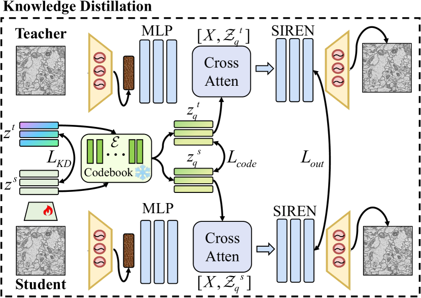
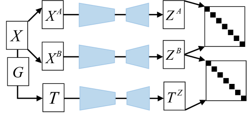
As delineated in Equation 1, our compression strategy fundamentally relies on the discrete prior features and continuous coordinate values , employing an INR network to fit a smooth function. In this context, we utilize a SIREN network for fitting purposes. Furthermore, we employ a knowledge distillation approach to condense the prior information from a more complex teacher model into a simplified student model. Our distillation process is bifurcated into two segments: aligning the intermediate discrete feature outputs and the final intensity estimation outputs between the teacher-student models as shown in Figure 2.
Intermediate Feature Alignment. In the first segment, the teacher model maintains its architecture as previously established, while the student model is subjected to a simplification process. We utilize the identical pre-trained network as a feature extractor for both models, the teacher model distinctively extracts high-frequency, low-frequency, and original image information. In contrast, the student model focuses solely on extracting features from the original image. Diverging from the teacher model’s approach, we have designed the feature extractor of the student model to be trainable. This ensures that the feature remains consistent with that of the teacher model. Both teacher and student models share a common codebook for nearest neighbor mapping as equation 5. Consequently, the loss is bifurcated into two pivotal components: discrete and continuous alignment. The discrete alignment is articulated as
| (9) |
where represents the discrete codebook of the teacher model, and corresponds to that of the student model. On the other hand, continuous alignment is described by the equation
| (10) |
where and represent the logits outputs of the teacher and student models, respectively. The temperature parameter plays a pivotal role in moderating the degree of softness in the probability distributions. The Kullback-Leibler (KL) divergence, denoted as , is utilized to measure the divergence between these probability distributions.
In our approach, the discrete alignment employs a Mean Squared Error (MSE) constraint, characterized as a hard constraint. In contrast, for continuous alignment, we apply a soft constraint. The primary objective of this soft constraint is to enable the student model to learn the probability distribution of the teacher model. This methodology of applying a soft constraint is particularly advantageous for model compression, allowing for a more efficient distillation process while preserving the essential characteristics of the teacher model’s predictive distribution.
Final Output Alignment. In the second segment, the alignment of the final outputs is meticulously orchestrated by matching the outputs of both the teacher and student models, as well as aligning them with the true values. This crucial step ensures a harmonized and coherent relationship among the student model, the teacher model, and the actual data. The alignment loss is mathematically formulated as
| (11) | ||||
where denotes the intensity of the original pixel in the input. Building upon this framework, the total loss function of our proposed methodology is encapsulated as
| (12) |
where represents the weighting coefficients assigned to each constituent loss function. Our training regimen commences with the initial training of the codebook and the teacher model. Subsequently, we harness the knowledge distillation technique to refine the training of the student model and further fine-tune the teacher model.
4 Experiments and Results
4.1 Implementation Details
Experiment Settings Our teacher model was trained on a cluster equipped with 8 NVIDIA RTX 3090 GPUs, with each GPU handling a batch size of 4. We employed three feature extractors, all pre-trained ResNet-50 models, which were kept frozen during the training to extract features of dimension 512. The wavelet transform was implemented using the OpenCV library, and the codebook size was set to 256. The teacher model underwent 800 epochs of training using the AdamW optimizer with an initial learning rate of 1e-5, optimized with a cosine annealing learning rate strategy.
For the student model, we focused on extracting knowledge from the teacher model, using an active ResNet-50 as the feature extractor for the original images. The total network parameters were kept at half the size of the teacher model. The student model underwent fine-tuning for 400 epochs on data blocks learned by the teacher model. The training process was managed using the AdamW optimizer, with an initial learning rate of 1e-5. Detailed information regarding hyperparameter settings and specific regularization techniques will be provided in the supplementary materials and our code repository. During decoding, we needed to additionally save codebook information and indices, hence the computation of the compression ratio includes these two parts.
Dataset. We evaluated the effectiveness of our method using CT and EM datasets. The CT data was sourced from the Medical Segmentation Decathlon (MSD) antonelli2022medical , comprising CT scans of three organs: Liver, Colon, and Spleen. Each voxel typically measures 1.001.002.5 mm, suitable for medium-level detail organ recognition. These organs are represented by 201, 190, and 61 high-precision medical slices respectively, and we cropped each slice into 64512512 blocks centered for network input.
On the other hand, for the biomedical dataset, we used the CREMI dataset heinrich2018synaptic , comprising serial section Transmission Electron Microscopy (ssTEM) images of Drosophila neural circuits. Since electron microscopy is highly sensitive to noise, these images contain many artifacts and missing sections. The voxel resolution is 4440 nm, capturing the complex details necessary for neural structure reconstruction. The dataset includes three samples, each containing a volume of 12512501250 voxels. Similarly, we selected a cropping size of 64512512.
Baseline Methods. To quantitatively assess our model’s performance, we employed two widely used metrics: Structural Similarity Index Measure (SSIM) and Peak Signal-to-Noise Ratio (PSNR). SSIM evaluates structural similarity, while PSNR measures pixel-level similarity, inversely related to Mean Squared Error (MSE). Our approach was benchmarked against traditional standards and neural representation methods, comparing it with state-of-the-art techniques.
We implemented standard codecs using FFMpeg and HM, including JPEG wallace1991jpeg , JPEG XL alakuijala2019jpeg , H.264 wiegand2003overview , and HEVC sullivan2012overview . Additionally, we evaluated data-driven models like DVC lu2019dvc and SSF agustsson2020scale with default settings. In neural representations, we considered SIREN sitzmann2020implicit , NeRF martin2021nerf , NeRV chen2021nerv , and TINC yang2023tinc . A key aspect of our analysis was highlighting neural representation techniques for precise compression ratio tuning. We used distortion curves and tested the CT dataset at compression ratios of 64, 128, 256, 512, and 1024, and the EM dataset at ratios of 4, 8, 12, 16, and 20.
For specific parameters, FFMpeg was used for JPEG with -q:v 2 for high quality and -q:v 10 for lower quality. For JPEG XL, we used -q 90 for high quality and -q 50 for lower quality. H.264 was encoded with FFMpeg at -crf 23 for medium quality and -crf 28 for lower quality. HEVC was configured in HM with -q 32 for medium quality and -q 37 for lower quality. These settings ensured a fair comparison of compression ratio and image quality.
4.2 Results
Our experimental evaluation is divided into two distinct scenarios: within-domain and cross-domain knowledge distillation, to comprehensively evaluate the effectiveness of our proposed method.
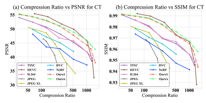
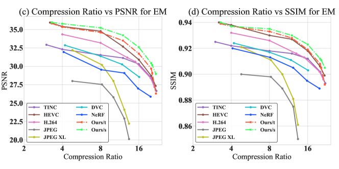
Within-Domain Results. In our within-domain experiments, the teacher model is trained and distilled within selected CT or EM datasets. Initially, the teacher model is trained on a specific subset of the dataset, encompassing all inherent structural information of the dataset. This robust model is then utilized to distill knowledge into the student model, which is subsequently fine-tuned on similar types of datasets. The distillation process leverages the complex details absorbed by the teacher model, with a special emphasis on preserving key high-resolution features critical for reconstruction tasks. The performance of the student model is benchmarked against the teacher model, with a particular focus on the preservation of detailed structural information and compression efficiency. Our experimental results are presented in Table 1, and the performance curves across various compression ratios are shown in Figure 3.
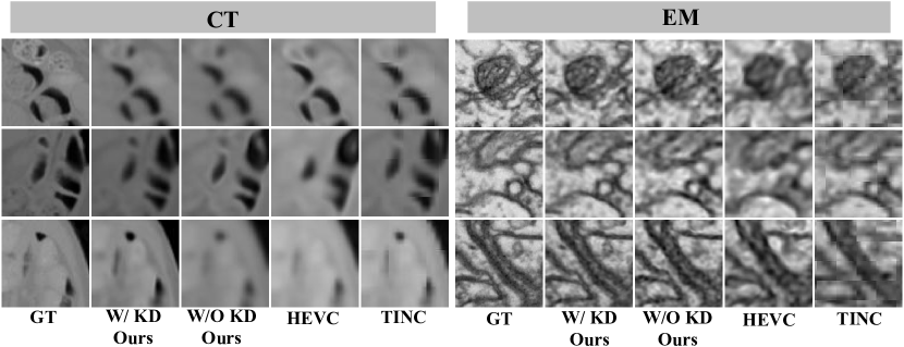
In the CT dataset, our approach achieved the best performance among similar INR methods and is comparable to commercial methods like HEVC. The performance of the model significantly improved after knowledge distillation. Notably, our approach is more resistant to distortion at high compression ratios, whereas HEVC experiences a drastic performance drop beyond a 1000 compression ratio. In the CREMI dataset, our method surpassed HEVC, and we observed a significant decline in the performance of INR-based approaches like TINC, likely due to their network structures causing overly smooth image recovery. This is unreasonable for EM images rich in high-frequency information. Our method, by introducing frequency information as a prior, mitigates this over-smoothing issue inherent in INR. Our visualization results are displayed in Figure 4.
| Method | Liver | Colon | Spleen | CREMI | ||||
|---|---|---|---|---|---|---|---|---|
| PSNR | SSIM | PSNR | SSIM | PSNR | SSIM | PSNR | SSIM | |
| TINC yang2023tinc | 45.81 | 0.9756 | 45.03 | 0.9744 | 45.35 | 0.9709 | 27.99 | 0.8427 |
| SIREN sitzmann2020implicit | 43.96 | 0.9602 | 44.54 | 0.9742 | 44.49 | 0.9689 | 28.54 | 0.8444 |
| NeRF martin2021nerf | 42.82 | 0.9528 | 39.37 | 0.9686 | 45.23 | 0.9740 | 27.70 | 0.8469 |
| NeRV chen2021nerv | 42.96 | 0.9546 | 39.91 | 0.9713 | 44.38 | 0.9700 | 26.71 | 0.8403 |
| JPEG wallace1991jpeg | 41.85 | 0.9654 | 37.36 | 0.9632 | 42.60 | 0.9610 | 25.26 | 0.8250 |
| JPEG XL alakuijala2019jpeg | 45.99 | 0.9773 | 44.12 | 0.9700 | 44.43 | 0.9645 | 28.71 | 0.8499 |
| H.264 wiegand2003overview | 44.03 | 0.9634 | 42.55 | 0.9724 | 45.41 | 0.9722 | 29.96 | 0.8478 |
| HEVC sullivan2012overview | 47.28 | 0.9835 | 48.21 | 0.9851 | 46.41 | 0.9769 | 30.41 | 0.8547 |
| DVC lu2019dvc | 42.48 | 0.9533 | 37.58 | 0.9664 | 43.34 | 0.9663 | 26.46 | 0.8360 |
| SSF agustsson2020scale | 45.05 | 0.9705 | 40.93 | 0.9714 | 45.42 | 0.9639 | 28.03 | 0.8449 |
| UniCompress(w/o KD) | 46.69 | 0.9791 | 46.90 | 0.9752 | 45.46 | 0.9730 | 30.25 | 0.8542 |
| UniCompress(w/ KD) | 47.08 | 0.9811 | 47.79 | 0.9812 | 46.32 | 0.9758 | 31.02 | 0.8601 |
| Source | Target | PSNR | SSIM | ||
|---|---|---|---|---|---|
| w/o KD | w/ KD | w/o KD | w/ KD | ||
| Colon | Liver | 46.69 | 47.47 (+0.78) | 0.9791 | 0.9834 (+0.0043) |
| Spleen | Liver | 46.69 | 47.12 (+0.43) | 0.9791 | 0.9821 (+0.0030) |
| Spleen | Colon | 46.90 | 47.34 (+0.44) | 0.9752 | 0.9801 (+0.0049) |
| Liver | Colon | 46.90 | 47.21 (+0.31) | 0.9752 | 0.9789 (+0.0037) |
| Liver | Spleen | 45.46 | 45.89 (+0.43) | 0.9730 | 0.9741 (+0.0011) |
| Colon | Spleen | 45.46 | 45.83 (+0.37) | 0.9730 | 0.9761 (+0.0031) |
Cross-Domain Results. In consideration of practical scenarios where the data requiring compression is often unknown, we ventured to extend the concept of knowledge distillation into the realm of cross-domain experiments. Specifically, we trained teacher models on datasets featuring different modalities and organs, subsequently distilling this prior knowledge into distinct organs or modalities to probe broader applicability and robustness. For our experiments, we selected CT datasets for mutual distillation, while EM datasets were excluded due to significant compression ratio differences.
The experimental results, as shown in Table 2, illustrate the average outcomes under varying compression ratios. Intriguingly, our findings reveal that cross-domain distillation enables the student models to surpass the average performance metrics of the teacher models. Remarkably, we observed that for the Liver dataset, the gains from cross-domain distillation even outperformed those within the same domain. This was attributed to the Liver dataset containing more background elements compared to the other two datasets, which may lead to insufficient discriminative information being introduced during the initial training phase of the teacher model using only the Liver dataset, thereby rendering minimal gains from knowledge distillation. Our results imply that this methodology can rapidly adapt to new datasets, a capability crucial in practical applications.
Comparison of Running Time. Traditional INR schemes, often tailored to overfit individual data points, significantly impeding encoding speed. Our method, UniCompress, achieves a 45 fold increase in encoding speed with only a marginal increase in decoding time. We have meticulously documented the time required for compression and decompression for each algorithm in our experiments, as presented in Supplementary Tables 7. The enhanced encoding speed of UniCompress is particularly beneficial in handling large volumes of medical imagery, significantly reducing compression time, a critical advancement in medical applications.
4.3 Ablation Studys
Frequency Domain Information Ablation Study. We employed wavelet transform to treat frequency domain information as a codebook prior. To validate the efficacy of this information, we conducted an ablation study as shown in Table 5. This table displays the performance of the un-distilled teacher model. We observed that all frequency domain information contributes to certain improvements. Notably, for complex images like those in CREMI, the high-frequency information showed a significant enhancement, yielding a 0.94 dB gain in PSNR compared to the baseline method.
Codebook Ablation Study. In our prior knowledge, additional feature dimensions and a larger codebook size contribute to more refined discriminative features. However, due to the need to store the codebook and indices at the decoding end, an excessively large codebook size can lead to a reduction in compression ratio. For downstream compression tasks, there exists a certain trade-off in setting these parameters. Therefore, we conducted an ablation study on the size of the codebook, as shown in Table 5. We tuned parameters that are suitable across two different modalities and found that a larger codebook size is more appropriate for complex EM data.
Ablation Study on knowledge distillation. We employ discrete codebook features, continuous intermediate features, and the final output to constrain the knowledge distillation process. An ablation study was conducted on these three components, with the results presented in Table 6. We observed that constraints on the final output and the discrete codebook have a more significant impact on the results. This could be attributed to these components’ ability to capture critical aspects of the learned representations, such as preserving crucial information through the distillation process and ensuring that the distilled model retains the essential characteristics of the teacher model. This emphasizes the importance of these constraints in achieving effective knowledge transfer.
5 Conclusion
In this study, we introduced “UniCompress”, a novel approach for the concurrent compression of multiple medical image datasets, integrating wavelet transforms with INR networks. Our method effectively encodes both spatial and frequency domain information, significantly enhancing compression ratios and data integrity preservation. Additionally, our technique of knowledge distillation demonstrates considerable improvement in compression speed and cross-domain applicability. Our experiments on complex datasets like CREMI and MSD show that UniCompress achieves substantial improvements over existing methods in terms of compression performance and efficiency, laying the groundwork for future advances in medical image processing.
References
- [1] Eirikur Agustsson, David Minnen, Nick Johnston, Johannes Balle, Sung Jin Hwang, and George Toderici. Scale-space flow for end-to-end optimized video compression. In Proceedings of the IEEE/CVF Conference on Computer Vision and Pattern Recognition, pages 8503–8512, 2020.
- [2] Jyrki Alakuijala, Ruud Van Asseldonk, Sami Boukortt, Martin Bruse, Iulia-Maria Com\textcommabelowsa, Moritz Firsching, Thomas Fischbacher, Evgenii Kliuchnikov, Sebastian Gomez, Robert Obryk, et al. Jpeg xl next-generation image compression architecture and coding tools. In Applications of Digital Image Processing XLII, volume 11137, pages 112–124. SPIE, 2019.
- [3] Michela Antonelli, Annika Reinke, Spyridon Bakas, Keyvan Farahani, Annette Kopp-Schneider, Bennett A Landman, Geert Litjens, Bjoern Menze, Olaf Ronneberger, Ronald M Summers, et al. The medical segmentation decathlon. Nature communications, 13(1):4128, 2022.
- [4] Tim Bruylants, Adrian Munteanu, and Peter Schelkens. Wavelet based volumetric medical image compression. Signal processing: Image communication, 31:112–133, 2015.
- [5] Michal Byra, Charissa Poon, Muhammad Febrian Rachmadi, Matthias Schlachter, and Henrik Skibbe. Exploring the performance of implicit neural representations for brain image registration. Scientific Reports, 13(1):17334, 2023.
- [6] Irem Cetin, Maialen Stephens, Oscar Camara, and Miguel A González Ballester. Attri-vae: Attribute-based interpretable representations of medical images with variational autoencoders. Computerized Medical Imaging and Graphics, 104:102158, 2023.
- [7] Hao Chen, Bo He, Hanyu Wang, Yixuan Ren, Ser Nam Lim, and Abhinav Shrivastava. Nerv: Neural representations for videos. Advances in Neural Information Processing Systems, 34:21557–21568, 2021.
- [8] Yinda Chen, Wei Huang, Xiaoyu Liu, Qi Chen, and Zhiwei Xiong. Learning multiscale consistency for self-supervised electron microscopy instance segmentation. In IEEE International Conference on Acoustics, Speech, and Signal Processing, 2023.
- [9] Yinda Chen, Wei Huang, Shenglong Zhou, Qi Chen, and Zhiwei Xiong. Self-supervised neuron segmentation with multi-agent reinforcement learning. In Proceedings of the Thirty-Second International Joint Conference on Artificial Intelligence, pages 609–617, 2023.
- [10] Yinda Chen, Che Liu, Wei Huang, Sibo Cheng, Rossella Arcucci, and Zhiwei Xiong. Generative text-guided 3d vision-language pretraining for unified medical image segmentation. arXiv preprint arXiv:2306.04811, 2023.
- [11] Yinda Chen, Che Liu, Xiaoyu Liu, Rossella Arcucci, and Zhiwei Xiong. Bimcv-r: A landmark dataset for 3d ct text-image retrieval. arXiv preprint arXiv:2403.15992, 2024.
- [12] Zhihao Duan, Ming Lu, Jack Ma, Yuning Huang, Zhan Ma, and Fengqing Zhu. Qarv: Quantization-aware resnet vae for lossy image compression. IEEE Transactions on Pattern Analysis and Machine Intelligence, 2023.
- [13] Patrick Esser, Robin Rombach, and Bjorn Ommer. Taming transformers for high-resolution image synthesis. In Proceedings of the IEEE/CVF conference on computer vision and pattern recognition, pages 12873–12883, 2021.
- [14] Zongyu Guo, Gergely Flamich, Jiajun He, Zhibo Chen, and José Miguel Hernández-Lobato. Compression with bayesian implicit neural representations. arXiv preprint arXiv:2305.19185, 2023.
- [15] Larissa Heinrich, Jan Funke, Constantin Pape, Juan Nunez-Iglesias, and Stephan Saalfeld. Synaptic cleft segmentation in non-isotropic volume electron microscopy of the complete drosophila brain. In Medical Image Computing and Computer Assisted Intervention–MICCAI 2018: 21st International Conference, Granada, Spain, September 16-20, 2018, Proceedings, Part II 11, pages 317–325. Springer, 2018.
- [16] Amirhossein Kazerouni, Reza Azad, Alireza Hosseini, Dorit Merhof, and Ulas Bagci. Incode: Implicit neural conditioning with prior knowledge embeddings. In Proceedings of the IEEE/CVF Winter Conference on Applications of Computer Vision, pages 1298–1307, 2024.
- [17] Jinhyuk Lee, Wonjin Yoon, Sungdong Kim, Donghyeon Kim, Sunkyu Kim, Chan Ho So, and Jaewoo Kang. Biobert: a pre-trained biomedical language representation model for biomedical text mining. Bioinformatics, 36(4):1234–1240, 2020.
- [18] Junnan Li, Dongxu Li, Silvio Savarese, and Steven Hoi. Blip-2: Bootstrapping language-image pre-training with frozen image encoders and large language models. arXiv preprint arXiv:2301.12597, 2023.
- [19] Pengju Liu, Hongzhi Zhang, Kai Zhang, Liang Lin, and Wangmeng Zuo. Multi-level wavelet-cnn for image restoration. In Proceedings of the IEEE conference on computer vision and pattern recognition workshops, pages 773–782, 2018.
- [20] Guo Lu, Wanli Ouyang, Dong Xu, Xiaoyun Zhang, Chunlei Cai, and Zhiyong Gao. Dvc: An end-to-end deep video compression framework. In Proceedings of the IEEE/CVF Conference on Computer Vision and Pattern Recognition, pages 11006–11015, 2019.
- [21] Ricardo Martin-Brualla, Noha Radwan, Mehdi SM Sajjadi, Jonathan T Barron, Alexey Dosovitskiy, and Daniel Duckworth. Nerf in the wild: Neural radiance fields for unconstrained photo collections. In Proceedings of the IEEE/CVF Conference on Computer Vision and Pattern Recognition, pages 7210–7219, 2021.
- [22] Yuhong Mo, Shaojie Li, Yushan Dong, Ziyi Zhu, and Zhenglin Li. Password complexity prediction based on roberta algorithm. Applied Science and Engineering Journal for Advanced Research, 3(3):1–5, 2024.
- [23] Albert Pumarola, Enric Corona, Gerard Pons-Moll, and Francesc Moreno-Noguer. D-nerf: Neural radiance fields for dynamic scenes. In Proceedings of the IEEE/CVF Conference on Computer Vision and Pattern Recognition, pages 10318–10327, 2021.
- [24] Vishwanath Saragadam, Daniel LeJeune, Jasper Tan, Guha Balakrishnan, Ashok Veeraraghavan, and Richard G Baraniuk. Wire: Wavelet implicit neural representations. In Proceedings of the IEEE/CVF Conference on Computer Vision and Pattern Recognition, pages 18507–18516, 2023.
- [25] Xinyu Shen, Qimin Zhang, Huili Zheng, and Weiwei Qi. Harnessing xgboost for robust biomarker selection of obsessive-compulsive disorder (ocd) from adolescent brain cognitive development (abcd) data.
- [26] Vincent Sitzmann, Julien Martel, Alexander Bergman, David Lindell, and Gordon Wetzstein. Implicit neural representations with periodic activation functions. Advances in neural information processing systems, 33:7462–7473, 2020.
- [27] Vincent Sitzmann, Michael Zollhöfer, and Gordon Wetzstein. Scene representation networks: Continuous 3d-structure-aware neural scene representations. Advances in Neural Information Processing Systems, 32, 2019.
- [28] Gary J Sullivan, Jens-Rainer Ohm, Woo-Jin Han, and Thomas Wiegand. Overview of the high efficiency video coding (hevc) standard. IEEE Transactions on circuits and systems for video technology, 22(12):1649–1668, 2012.
- [29] Zhiwei Tang, Tsung-Hui Chang, Xiaojing Ye, and Hongyuan Zha. Low-rank matrix recovery with unknown correspondence. In Robin J. Evans and Ilya Shpitser, editors, Proceedings of the Thirty-Ninth Conference on Uncertainty in Artificial Intelligence, volume 216 of Proceedings of Machine Learning Research, pages 2111–2122. PMLR, 31 Jul–04 Aug 2023.
- [30] Zhiwei Tang, Dmitry Rybin, and Tsung-Hui Chang. Zeroth-order optimization meets human feedback: Provable learning via ranking oracles. In The Twelfth International Conference on Learning Representations, 2024.
- [31] Zhiwei Tang, Yanmeng Wang, and Tsung-Hui Chang. z-signfedavg: A unified stochastic sign-based compression for federated learning. In Proceedings of the AAAI Conference on Artificial Intelligence, volume 38, pages 15301–15309, 2024.
- [32] Aaron Van Den Oord, Oriol Vinyals, et al. Neural discrete representation learning. Advances in neural information processing systems, 30, 2017.
- [33] John D Villasenor, Benjamin Belzer, and Judy Liao. Wavelet filter evaluation for image compression. IEEE Transactions on image processing, 4(8):1053–1060, 1995.
- [34] Gregory K Wallace. The jpeg still picture compression standard. Communications of the ACM, 34(4):30–44, 1991.
- [35] Ji Wang, Weidong Bao, Lichao Sun, Xiaomin Zhu, Bokai Cao, and S Yu Philip. Private model compression via knowledge distillation. In Proceedings of the AAAI Conference on Artificial Intelligence, volume 33, pages 1190–1197, 2019.
- [36] Thomas Wiegand, Gary J Sullivan, Gisle Bjontegaard, and Ajay Luthra. Overview of the h. 264/avc video coding standard. IEEE Transactions on circuits and systems for video technology, 13(7):560–576, 2003.
- [37] Dongmei Xue, Haichuan Ma, Li Li, Dong Liu, Zhiwei Xiong, and Houqiang Li. Dbvc: An end-to-end 3-d deep biomedical video coding framework. IEEE Transactions on Circuits and Systems for Video Technology, 2023.
- [38] Runzhao Yang. Tinc: Tree-structured implicit neural compression. In Proceedings of the IEEE/CVF Conference on Computer Vision and Pattern Recognition, pages 18517–18526, 2023.
- [39] Runzhao Yang, Tingxiong Xiao, Yuxiao Cheng, Qianni Cao, Jinyuan Qu, Jinli Suo, and Qionghai Dai. Sci: A spectrum concentrated implicit neural compression for biomedical data. In Proceedings of the AAAI Conference on Artificial Intelligence, volume 37, pages 4774–4782, 2023.
- [40] Runzhao Yang, Tingxiong Xiao, Yuxiao Cheng, Anan Li, Jinyuan Qu, Rui Liang, Shengda Bao, Xiaofeng Wang, Jue Wang, Jinli Suo, et al. Sharing massive biomedical data at magnitudes lower bandwidth using implicit neural function. bioRxiv, pages 2022–12, 2022.
- [41] Ye Zhang, Yulu Gong, Dongji Cui, Xinrui Li, and Xinyu Shen. Deepgi: An automated approach for gastrointestinal tract segmentation in mri scans. arXiv preprint arXiv:2401.15354, 2024.
- [42] Yunlong Zhang, Chenxin Li, Xin Lin, Liyan Sun, Yihong Zhuang, Yue Huang, Xinghao Ding, Xiaoqing Liu, and Yizhou Yu. Generator versus segmentor: Pseudo-healthy synthesis. In Medical Image Computing and Computer Assisted Intervention–MICCAI 2021: 24th International Conference, Strasbourg, France, September 27–October 1, 2021, Proceedings, Part VI 24, pages 150–160. Springer, 2021.
- [43] Yanfeng Zhou, Jiaxing Huang, Chenlong Wang, Le Song, and Ge Yang. Xnet: Wavelet-based low and high frequency fusion networks for fully-and semi-supervised semantic segmentation of biomedical images. In Proceedings of the IEEE/CVF International Conference on Computer Vision, pages 21085–21096, 2023.
- [44] Weihao Zhuang, Tristan Hascoet, Xunquan Chen, Ryoichi Takashima, Tetsuya Takiguchi, et al. Optical flow regularization of implicit neural representations for video frame interpolation. APSIPA Transactions on Signal and Information Processing, 12(1), 2022.
Appendix
Appendix A Theoretical Advantages of INR Compression
Assumption A.1.
Suppose we have an image dataset consisting of samples, where each sample is an image of size with channels. We assume that these images are independently and identically distributed (i.i.d.) samples from some unknown distribution .
We consider using Implicit Neural Representations (INR) and Variational Autoencoders (VAE) for image compression. For INR, we define an encoder that maps an image to a -dimensional vector in the latent space, and a decoder that maps a latent vector back to the image space. The training objective of INR is to minimize the reconstruction error:
| (13) |
For VAE, we introduce a prior distribution (usually taken to be a standard Gaussian), and define an encoder and a decoder . The training objective of VAE is to maximize the evidence lower bound (ELBO):
| (14) |
Theorem A.2.
Under Assumption A.1, suppose INR and VAE have the same compression rate, i.e., . Denote the optimal parameters of INR and VAE as and , respectively. Then,
| (15) |
In other words, under the same compression rate, the reconstruction error of INR is no greater than that of VAE.
Proof.
For VAE, we have:
This follows from the law of total expectation and the fact that for any random vector .
On the other hand, for INR, we have:
Now, let’s compare the second terms in the above two expressions. For VAE, we have:
where the last inequality follows from Jensen’s inequality.
For INR, we have:
where denotes the angle between vectors and , and is the maximum possible angle between any pair of vectors in the dataset.
Comparing the bounds for VAE and INR, we observe that if
| (16) |
then the second term in the INR bound will be larger than that in the VAE bound, implying a smaller reconstruction error for INR.
Now, let us compare the third terms in the VAE and INR bounds. For VAE, we have:
| (17) |
while for INR, we have:
| (18) |
If the expected squared norm of the reconstructed images under INR is smaller than that under VAE, i.e.,
| (19) |
then the third term in the INR bound will be smaller than that in the VAE bound.
In summary, under the conditions:
the reconstruction error of INR will be smaller than that of VAE under the same compression rate. These conditions essentially require that the INR decoder generates images with smaller expected squared norm and higher cosine similarity to the original images compared to the VAE decoder.
∎
The key idea behind this proof is to compare the bounds on the reconstruction errors of INR and VAE by analyzing the terms in their respective expressions. The conditions derived in the proof provide insights into when INR can achieve better compression performance than VAE. Intuitively, if the INR decoder can generate images that are more similar to the original images and have smaller magnitudes compared to the VAE decoder, then INR will have a lower reconstruction error.
It is worth noting that the conditions in the proof are sufficient but not necessary for INR to outperform VAE. In practice, the actual performance of INR and VAE will depend on various factors such as the network architectures, training procedures, and the specific dataset. Nevertheless, this theoretical analysis sheds light on the potential advantages of INR over VAE in terms of image compression.
Appendix B Dataset Information
Our experiments encompass three CT datasets and one Electron Microscopy (EM) dataset. Table 3 provides detailed information on all these datasets. To standardize the input size for our network, we uniformly cropped the datasets to volumes of 64512512. The CREMI dataset can be accessed at https://cremi.org/data/, and the MSD dataset is available at http://medicaldecathlon.com/.
| Name | Category | Species | Position | Characteristic | Bit depth | w/o sign | Resolution | Slice counts |
|---|---|---|---|---|---|---|---|---|
| CREMI | EM, biological | adult drosophila | brain | anisotropy | 8 | unsigned | 125×1250×1250 | / |
| CT-Liver | CT, medical | human | liver | anisotropy | 32 | signed | 588×512×512 | 201 |
| CT-Lung | CT, medical | human | lung | anisotropy | 32 | signed | 241×512×512 | 96 |
| CT-Spleen | CT, medical | human | spleen | anisotropy | 32 | signed | 94×512×512 | 61 |
Appendix C Numerical Results of the Ablation Study
In this section, we provide the tables containing the numerical results of the ablation experiments.
|
|
|||||||||||||||||||||||||||||||||||||||||||||||||||||||||||||||||||||||||||||||||
| Spleen | CREMI | |||||
|---|---|---|---|---|---|---|
| PSNR | SSIM | PSNR | SSIM | |||
| 46.01 | 0.9715 | 30.79 | 0.8569 | |||
| 46.27 | 0.9741 | 30.93 | 0.8591 | |||
| 46.11 | 0.9722 | 30.84 | 0.8574 | |||
| 46.32 | 0.9758 | 31.02 | 0.8601 | |||
Appendix D Compression Efficiency
Beyond visual metrics, the time consumed for data encoding and decoding is a crucial measure of a compression algorithm’s efficacy. We evaluated the encoding and decoding times for all comparison baselines discussed in the main text. Specifically, the decoding time refers to the duration required to decode 1,000 data blocks. The results are presented in Table 7. Our approach demonstrates a 45 times faster encoding process for both CT and EM datasets compared to common INR compression schemes like TINC and SIREN. This significant speed-up in encoding can greatly enhance efficiency in large-scale medical image compression, while incurring only a minimal increase in decoding time.
| CT | EM | ||||
| Compression | Decompression | Compression | Decompression | ||
| Method | (Seconds) | x1k(seconds) | (Seconds) | x1k(seconds) | |
| UniCompress(w/ KD) | 571.3 | 313.7 | 581.8 | 321.9 | |
| TINC [38] | 2271 | 241.9 | 2672 | 279.1 | |
| SIREN [26] | 2013 | 200.8 | 2319 | 223.7 | |
| NeRV [7] | 2412 | 197.3 | 2672 | 201.9 | |
| INR based | NeRF [21] | 526.7 | 102.4 | 769.6 | 124.4 |
| H.264 [36] | 1.730 | 381.3 | 2.130 | 448.6 | |
| Commercial | HEVC [28] | 1.070 | 697.3 | 2.130 | 658.9 |
| DVC [20] | 62.39 | 387.1 | 68.91 | 399.4 | |
| Data driven | SSF [1] | 6.987 | 397.0 | 6.127 | 119.7 |
Appendix E Pretraining Approach
In pursuit of extracting 3D visual representations from medical images, we introduce a vision-language pretraining approach that leverages large language models for generating textual descriptions of 3D images. This framework encompasses several key components and learning objectives, and can be summarized as Figure 5 .
E.1 Text Generation
The text generation process involves a generator , which is initially loaded with BLIP2’s [18] pretrained weights and further fine-tuned on the BIMCV dataset (a medical image-text pair dataset). This generator produces a sequence of tokens for each 3D medical image . The conditional probability of each token is modeled as
| (20) |
where and are the weights and biases of the output layer, and represents the hidden state at time step .
E.2 Visual-Textual Representation Learning
The framework employs an image encoder and a text encoder to learn visual-textual representations. The text encoder is initialized with the weights from BioBERT [17] and is frozen during pretraining. For a batch of image-text pairs , the feature representations are computed as and . A contrastive learning objective is used to predict the matched pair while ensuring significant separation of negative pairs.
E.3 3D Visual Representation Learning
To address the challenges of 1-to-n positive-negative pairings in 3D visual learning, we employ a negative-free learning objective. This involves generating two distinct views and of the medical volume through data augmentation. The goal is to minimize the off-diagonal elements and maximize the diagonal elements of the cross-correlation matrix . The loss function is formulated as
| (21) |
where and are non-negative hyperparameters, and and represent the normalized embeddings of the first and second views, respectively. Ultimately, the pretrained encoders are utilized to extract semantic information from high-frequency, low-frequency, and original images.
E.4 Ablation Experiment of Pretraining
In the main text, we mention the use of a frozen pretrained network for feature extraction. Freezing the network weights aids in stabilizing the training process of the model. Furthermore, vision-language pretraining methods have been validated as effective means for image feature extraction. In this section, we conduct ablation experiments, the results of which are shown in Table 8. We observe that activating the feature extraction weights during the training phase of the teacher model leads to failure in image reconstruction. This could be attributed to an insufficient number of epochs set, preventing adequate fitting to the codebook features. Meanwhile, the pretrained network substantially aids in feature extraction, significantly enhancing the reconstruction results.
| Freeze | Pretrain | Spleen | CREMI | ||
|---|---|---|---|---|---|
| PSNR | SSIM | PSNR | SSIM | ||
| 13.49 | 0.3142 | 12.71 | 0.2984 | ||
| 41.51 | 0.9312 | 24.91 | 0.7841 | ||
| 45.46 | 0.9730 | 30.25 | 0.8542 | ||
Appendix F Algorithm Pseudocode
The source code for our paper is provided in the supplementary materials. For ease of understanding, this section presents the pseudocode format of the algorithm proposed in our paper as Algorithm 1 and 2.
In this pseudocode, , , , and represent the specific loss functions used in the paper. Similarly, , , and are hyperparameters that need to adjust based on the specifics.
Appendix G Parameter Meaning and Hyperparameter Setting
The meanings of all parameters mentioned in our paper are detailed in Table 9. For the hyperparameters referenced in the main text, please refer to the code provided by us.
Appendix H Social Impact
In this study, we introduce UniCompress, a pioneering approach to multi-data medical image compression, combining Implicit Neural Representation (INR) networks with knowledge distillation techniques for enhanced efficiency and speed. We recognize that efficient image compression is vital for the sustainable development of the healthcare industry amid surging medical data volumes [25]. UniCompress not only reduces storage and transmission costs but could also improve diagnostic efficiency by decreasing data transfer times, which is crucial for telemedicine and emergency medical scenarios.
Ethically, we prioritize patient privacy and data security in developing and applying UniCompress, ensuring the compression process does not compromise image quality, thus maintaining the accuracy and reliability of medical diagnoses.
Appendix I Limitations
Despite demonstrating effectiveness across various medical image datasets, we acknowledge certain technical limitations of UniCompress. First, the current INR networks may not fully preserve details in images with high dynamic ranges and complex textures, especially in high-frequency areas. Second, quantization loss in the knowledge distillation process could lead to incomplete learning of the teacher model’s knowledge in some cases. Moreover, our model’s generalizability in handling large-scale datasets, especially diverse data from different medical institutions and devices, needs improvement.
Appendix J Future Works
To address these limitations, we plan to explore: (1) developing new INR architectures for better capturing and retaining high-frequency image information while maintaining compression efficiency; (2) optimizing knowledge distillation algorithms for more precise knowledge transfer and reduced information loss; (3) researching adaptive quantization strategies to balance compression ratios and image quality; (4) enhancing model generalizability to adapt to varied medical image data sources and qualities; (5) exploring interpretability of deep learning models for medical professionals to understand the decision-making in the compression process.
We anticipate these future efforts will further enhance UniCompress’s performance, making it a robust tool in medical image compression and contributing significantly to global health initiatives.
| Symbol | Meaning |
|---|---|
| Number of volumetric medical images to compress | |
| The -th volumetric medical image | |
| Spatial coordinates | |
| Prior features of the -th image block | |
| Parameters of the INR network | |
| Predicted intensity value at coordinate | |
| High-frequency information | |
| Low-frequency information | |
| Raw image | |
| Pre-trained network for feature extraction | |
| , , | High-frequency, low-frequency, and raw image features, respectively |
| , , | Attention weights for high-frequency, low-frequency, and raw image features, respectively |
| Quantized representation | |
| Weighting factor for quantization loss | |
| Reconstruction loss | |
| Quantization loss | |
| Total loss function | |
| Codebook alignment loss | |
| Knowledge distillation loss | |
| Output alignment loss | |
| Final total loss function | |
| Temperature parameter for KL divergence | |
| Weighting coefficients for balancing different loss functions | |
| Dimension of the codebook | |
| Set of all codewords in the codebook | |
| , | Discrete codebook of the student and teacher models, respectively |
| , | Logits outputs of the student and teacher models, respectively |
| , | Student and teacher models, respectively |
| Input data |