Locality, Correlations, Information, and non-Hermitian Quantum Systems

Abstract

Local non-Hermitian (NH) quantum systems generically exhibit breakdown of Lieb-Robinson (LR) bounds, motivating study of whether new locality measures might shed light not seen by existing measures. In this paper we discuss extensions of the connected correlation function (CC) as measures of locality and information spreading in both Hermitian and NH systems. We find that in Hermitian systems, $\delta\rho=\rho-\rho_{A}\otimes\rho_{B}$ can be written as a linear combination of CCs, allowing placement of a LR bound on $\|\delta\rho\|_{2}$, which we show generically extends to a LR bound on mutual information. Additionally, we extend the CC to NH systems in a form that recovers locality, and use the metric formalism to derive a modified CC which recovers not just locality but even LR bounds. We find that even with these CCs, the bound on $\|\delta\rho\|_{2}$ breaks down in certain NH cases, which can be used to place a necessary condition on which NH Hamiltonians are capable of nonlocal entanglement generation. Numerical simulations are provided by means of exact diagonalization for the NH Transverse-Field Ising Model, demonstrating both breakdown and recovery of LR bounds.

I Introduction

Though there exist a number of approaches for studying conditional time evolutions, description as a non-Hermitian (NH) Hamiltonian Ashida et al. (2020) reveals unique phenomena such as phase transitions without gap closing Matsumoto et al. (2020), exceptional points Matsumoto et al. (2022); Gopalakrishnan and Gullans (2021), and Lieb-Robinson (LR) bound violations Matsumoto et al. (2020); Ashida and Ueda (2018). LR bounds limit the speed of operator growth under non-relativistic local Hamiltonians Lieb and Robinson (1972); Nachtergaele and Sims (2006a); Bravyi et al. (2006) and local Lindbladians Poulin (2010), and are intimately related to many other results such as exponential decay of correlations Hastings and Koma (2006); Nachtergaele and Sims (2006a) and generation of topological order Bravyi et al. (2006), making their violation in local NH systems surprising. Counterintuitively, evolution under NH Hamiltonians may generate less entanglement than under their Hermitian counterparts Barch et al. (2023); Gopalakrishnan and Gullans (2021). This motivates questioning whether NH systems truly have long-range interactions, or if metrics designed for CPTP time evolution simply fail to capture the structure of locality in NH systems. We provide evidence towards the latter, by constructing a modified connected correlation function (CC) which obeys LR bounds even in NH systems while still acting as a faithful measure of entanglement.

CCs are commonly used as locality measures, and are connected to a range of topics such as chaoticity Gharibyan et al. (2020) and criticality Matsumoto et al. (2022). Previous work has shown a LR bound on standard Bravyi et al. (2006) and $n$-partite Tran et al. (2017) CCs, and demonstrated a connection between CCs and entanglement measures such as mutual information Tran et al. (2017); Wolf et al. (2008); Kudler-Flam et al. (2023); Scalet et al. (2021). As we show here, the difference $\delta\rho=\rho-\rho_{A}\otimes\rho_{B}$ can be not only bounded but written as a sum of CCs, extending the previously mentioned CC LR bound to functions of $\delta\rho$. In particular, we show that mutual information can generically be upper bounded by a multiple of $\|\delta\rho\|_{2}$, and thus by an LR bound (Eq. 26).

As the traditional CC loses its usual locality properties in NH systems, we instead consider two extensions. The first is a connected version of the correlator in Ref. Sergi and Zloshchastiev (2015), and reduces to the standard CC in the Hermitian limit. The second is motivated by the metric formalism of NH systems Mostafazadeh (2002, 2003); Ju et al. (2019); Karuvade et al. (2022), and is the CC in a modified Hilbert space in which the system is Hermitian. While both recover the desired locality properties and can be used as measures of entanglement, the latter is further shown to obey LR bounds in NH systems. Previous works have addressed disconnected correlators in NH systems, but these do not have the same locality properties as their connected counterparts Sergi and Zloshchastiev (2015); Matsumoto et al. (2022). To our knowledge this is the first extension of connected correlators to NH systems, and the first proof of any form of LR bound in local NH systems.

A background on relevant work in LR bounds, CCs, and NH systems is provided in Sec. II. In Sec. III we construct the two modified CCs and discuss their properties. In Sec. IV we relate them to entanglement by writing $\delta\rho$ as a sum of CCs, and show that this term generically upper bounds mutual information. Proof of LR bounds in NH systems for the new CCs is given in Sec. V. In Sec. VI we discuss two applications: bounding the class of NH Hamiltonians capable of generating long range entanglement, and measurement of CCs as POVMs. Finally in Sec. VII we discuss significance of results and prospects for future study. The appendix contains various results including extension of the CC LR bound to the unequal time case (A), $n$-partite extension of modified CCs (B), bounding mutual information in terms of $\|\delta\rho\|_{2}$ and decomposition of $\delta\rho$ in terms of modified CCs (C), additional results on LR bounds (D), and an example case of using a NH Hamiltonian to generate long range entanglement (E).

II Background

II.1 Lieb-Robinson Bounds

Even in nonrelativistic local quantum systems, there exists an effective lightcone limiting the spread of operator growth, known as the Lieb-Robinson (LR) bound  Lieb and Robinson (1972); Nachtergaele and Sims (2006a); Bravyi et al. (2006); Poulin (2010). This bound states that for a quantum system evolving under a local Hamiltonian $H$,

$$\left\|[O_{A}(t),O_{B}]\right\|\leq cN_{\text{min}}\|O_{A}\|\|O_{B}\|e^{-\frac{L-vt}{\xi}}$$ (1)

where $O_{A}(t)=U^{\dagger}_{t}O_{A}U_{t}$, $U_{t}=e^{-iHt}$, and $O_{A},O_{B}$ are any local operators initially supported on subsystems $A,B$ of distance $L$ apart. Additionally, $N_{\text{min}}=\text{min}\{|A|,|B|\}$, and $c,\xi$, and $v$ are system dependant constants.

This arises because, by definition, we can decompose a local Hamiltonian into a sum of local terms as $H=\sum_{R}H_{R}$ where $\{R\}$ are a set of subsystems of the quantum system whose locality is independent of system size. At time zero, the infinitesimal Heisenberg time evolution of $O_{A}$ is

$$\dot{O}_{A}\big{|}_{t=0}=i[H,O_{A}]=i\sum_{R\cap A\neq\varnothing}[H_{R},O_{A}]$$

as commutator terms for which $R\cap A=\varnothing$ vanish. After some small time $dt$, as each $H_{R}$ is local, $O_{A}(dt)$ will, to first order, be local on subsystem $\cup_{R\cap A\neq\varnothing}R$, and the process repeats.

This result was extended to show that one can also place a LR bound on the norm difference between an operator and its restriction onto a lightcone Bravyi et al. (2006). For some initially local operator $O_{A}$, pick some $l$ and let $S$ be the “spacelike” region, i.e. the region of subsystems with distance at least $l$ from $A$. Then we can define the restriction of $O_{A}(t)$ onto a lightcone of radius $l$ around $A$ as

$$O_{A}^{l}(t)\equiv\text{Tr}_{S}[O_{A}(t)]\otimes\frac{\mathbb{I}_{S}}{\text{Tr}[\mathbb{I}_{S}]}$$ (2)

It was shown in Ref. Bravyi et al. (2006) that for $\|O_{A}\|\leq 1$,

$$\|O_{A}(t)-O_{A}^{l}(t)\|\leq c|A|e^{-\frac{l-vt}{\xi}}$$ (3)

for the same $c,v,\xi$ as the original LR bound.

Interestingly, the LR bound breaks down when $H$ is instead a local NH Hamiltonian Matsumoto et al. (2020). We repeat the argument here for completeness. Consider a Hamiltonian $H=\sum_{R}H_{R}+i\Gamma_{R}$ composed of Hermitian $H_{R}$ and $\Gamma_{R}$, acting on local regions $R$. The infinitesimal time evolution of $O_{A}$ at time zero under this Hamiltonian is

$$\dot{O}_{A}\big{|}_{t=0} =iH^{\dagger}O_{A}-iO_{A}H$$

$$=i\sum_{R\cap A\neq\varnothing}[H_{R},O_{A}]-\sum_{R}\{\Gamma_{R},O_{A}\}.$$

While $[H_{R},O_{A}]=0$ for $R\cap A=\varnothing$ at $t=0$, the same does not hold for $\{\Gamma_{R},O_{A}\}$, which can in general cause nonlocal growth of $O_{A}$, and breakdown of the LR bound. This breakdown is related to non-unitality of the evolution, as highlighted by considering product non-Unitary time evolution operator $U=U_{A}\otimes U_{B}$. Here,

$$(U_{A}\otimes U_{B})^{\dagger}O_{A}(U_{A}\otimes U_{B})=(U_{A}^{\dagger}O_{A}U_{A})\otimes(U^{\dagger}_{B}U_{B})$$

which is no longer local on $A$.

II.2 Correlation Functions

The traditional CC for arbitrary operators $O_{1},O_{2}$ is given by

$$\langle O_{1},O_{2}\rangle_{c}=\langle O_{1}O_{2}\rangle-\langle O_{1}\rangle\langle O_{2}\rangle$$ (4)

where $\langle\ \cdot\ \rangle=\text{Tr}[\rho\ \cdot\ ]$ denotes expectation value w.r.t. some state $\rho$, which when ambiguous will be denoted explicitly by $\langle\ \cdot\ \rangle_{\rho}$. This can be extended to the unequal-time CC:

$$\langle O_{1}(t),O_{2}(t^{\prime})\rangle_{c}=\langle O_{1}(t)O_{2}(t^{\prime})\rangle-\langle O_{1}(t)\rangle\langle O_{2}(t^{\prime})\rangle$$ (5)

When $t=t^{\prime}$ this is equivalent to Eq. 4 on time evolved state $\rho(t)$.

II.2.1 Connected Correlators and Mutual Information

Unlike the disconnected correlator $\langle O_{A}O_{B}\rangle$, the CC is always zero for product states $\rho_{A}\otimes\rho_{B}$. In fact, the CC between any disjoint operators $O_{A},O_{B}$ acting on subsystems $A,B$ can be upper bounded in terms of the mutual information between the two subsystems Wolf et al. (2008):

$$\frac{|\langle O_{A},O_{B}\rangle_{c}|^{2}}{2\|O_{A}\|^{2}\|O_{B}\|^{2}}\leq I(A;B)$$ (6)

This result has been extended to a family of $\alpha$-Rényi mutual information measures Scalet et al. (2021); Kudler-Flam et al. (2023). Additionally, it was shown that the relationship is bidirectional for $\alpha=1/2$, in that the Rényi mutual information can be upper bounded by a sum of CCs Kudler-Flam et al. (2023). In Sec. IV we extend this result to traditional mutual information, and show that $I(A;B)$ itself can be upper bounded in terms of a sum of CCs in certain generic cases. This is achieved by bounding it in terms of $\delta\rho=\rho-\rho_{A}\otimes\rho_{B}$, itself a quantifier of entanglement, which be written as a sum of CCs. The resulting proof is an extension of a result from Ref. Tran et al. (2017) which shows that a state is product across a bipartition iff all CCs for operators on separate sides of the bipartition are zero. I.e. that

$$\begin{split}\rho=\rho_{A}\otimes\rho_{B}&\Leftrightarrow\langle O_{A},O_{B}\rangle_{c}=0\\ \forall O_{A}\in\mathscr{L(H}_{A})&,O_{B}\in\mathscr{L(H}_{B})\end{split}$$ (7)

II.2.2 LR Bounds for Connected Correlators

When $\rho$ exhibits finite correlation length, i.e. $\langle O_{A},O_{B}\rangle_{c}\leq\tilde{c}\ e^{-\frac{L}{\chi}}$ for system-dependent correlation length $\chi$, the LR bound on operators can be extended to one on CCs Bravyi et al. (2006); Tran et al. (2017). This is the case in, e.g., ground states of gapped local Hamiltonians Nachtergaele and Sims (2006a). Using Eq. 3 we can bound

$$\begin{split}&\big{|}\langle O_{A}(t),O_{B}(t)\rangle_{c}\big{|}\\ &\leq\left|\langle O_{A}^{l}(t),O_{B}^{l}(t)\rangle_{c}\right|+c\left(|A|+|B|\right)e^{\frac{l-vt}{\xi}}\\ &\leq\tilde{c}\ e^{-\frac{L-2l}{\chi}}+c(|A|+|B|)e^{-\frac{l-vt}{\xi}}\\ &\leq\bar{c}\ e^{-\frac{L-2vt}{\chi^{\prime}}}\end{split}$$ (8)

for $\bar{c}=\tilde{c}+c(|A|+|B|)$, $\chi^{\prime}=\chi+2\xi$, and the optimal $l=(\chi vt+\xi L)/\chi^{\prime}$. This extends to the $n$-partite case as well Tran et al. (2017). Additionally, as shown in Appendix A, this generalizes to the unequal-time case as

$$|\langle O_{A}(t),O_{B}(t^{\prime})\rangle_{c}|\leq\bar{c}\ e^{-\frac{L-v(t+t^{\prime})}{\chi^{\prime}}}$$ (9)

II.3 Non-Hermitian Quantum Mechanics

The paradigmatic conditional evolution motivating NH quantum mechanics is the no-jump trajectory Ashida et al. (2020); Brun (2002). Consider a state $\rho$ evolving under the standard Lindblad equation:

$$\dot{\rho}=-i[H,\rho]+\sum_{a}\left(L_{a}\rho L_{a}^{\dagger}-\frac{1}{2}\{L_{a}^{\dagger}L_{a},\rho\}\right).$$ (10)

While the first and third terms generate time evolution within a single quantum trajectory, the second term $L_{a}\rho L_{a}^{\dagger}$ corresponds to jumps between quantum trajectories. Postselecting out such jumps effectively removes this term, and the resulting evolution can be described by a NH effective Hamiltonian

$$H_{\mathrm{eff}}=H-\frac{i}{2}\sum_{a}L_{a}^{\dagger}L_{a}.$$ (11)

The resulting time evolution operator $U_{t}=e^{-iH_{\mathrm{eff}}t}$ is no longer Unitary, and the resulting time evolution is completely positive but no longer trace-preserving. Thus in order to interpret the output as states, the time evolution must be manually trace-normalized:

$$\rho(t)=\frac{U_{t}\rho U_{t}^{\dagger}}{\text{Tr}[U_{t}\rho U_{t}^{\dagger}]}$$ (12)

This is equivalent to normalization in the Bayes rule for conditional probability distributions, and comes from decay of the total probability of the conditional trajectory Ashida and Ueda (2018). For this reason the denominator is only zero when the trajectory occurs with probability zero, making this case unphysical. Notice that normalization also makes $\rho(t)$ invariant under constant shifts in $H$ both real and imaginary.

II.3.1 Metric Formalism

A Hamiltonian is said to be pseudo-Hermitian or $PT$-Symmetric if there exists Hermitian (generally non-unique) $\eta$ such that $H^{\dagger}\eta=\eta H$. A satisfying $\eta$ is referred to as a metric, as it defines a modified inner product, $\langle\psi,\phi\rangle_{\eta}\equiv\langle\psi|\eta|\phi\rangle$, under which $H$ is Hermitian Bender and Boettcher (1998); Bender et al. (2002); Mostafazadeh (2002). Eigenvalues of pseudo-Hermitian $H$ come in complex conjugate pairs. If there further exists a positive definite $\eta$, then $H$ is said to be quasi-Hermitian or $PT$-unbroken and is guaranteed to have real eigenvalues. In this latter case we can decompose

$$H=SH_{0}S^{-1}$$ (13)

for Hermitian $S$ and $H_{0}$, where $H_{0}$ is isospectral to $H$. The similarity transform under $S=\eta^{-1/2}$ is sometimes referred to as the Dyson map Fring and Moussa (2016); Dyson (1956). In this case we can also decompose $U_{t}=SV_{t}S^{-1}$, for Unitary $V_{t}=e^{-iH_{0}t}$. Note that Hamiltonians resulting from Eq. 11 cannot be properly pseudo-Hermitian, but can be up to an overall imaginary shift, which generates equivalent normalized dynamics.

As an alternative to treating NH Hamiltonians as effective, one can view them as fundamental, acting in a modified Hilbert space $\mathscr{H}_{\eta}$ with inner product $\langle\cdot,\cdot\rangle_{\eta}$; this latter approach is referred to as the metric formalism Mostafazadeh (2002). In this case $S$ acts as a map from the traditional Hilbert space $\mathscr{H}$ to $\mathscr{H}_{\eta}$, which is Unitary in the sense that $\langle S\psi,S\phi\rangle_{\eta}=\langle\psi|S\eta S|\phi\rangle=\langle\psi|\phi\rangle$. The two approaches to NH physics motivate two different extensions of CCs, which will both be considered in this paper.

II.4 Non-Hermitian Transverse-Field Ising Model

Simulations in this paper use the 1D Imaginary Transverse-field Ising model (TFIM), a NH extension of the paradigmatic TFIM with well studied entanglement phases Gopalakrishnan and Gullans (2021); Biella and Schiró (2021); Barch et al. (2023); Matsumoto et al. (2020). The Hamiltonian is:

$$H=J\sum\limits_{j=1}^{L-1}\sigma_{j}^{z}\sigma_{j+1}^{z}+\sum\limits_{j=1}^{L}\left(g\sigma_{j}^{x}+h\sigma_{j}^{z}+i\gamma\sigma_{j}^{y}\right),$$ (14)

In the Hermitian ($\gamma=0$) limit, the model is integrable when $g$ or $h$ is $0$ and chaotic otherwise, in that it obeys random matrix spectral statistics and volume-law eigenstate entanglement Bañuls et al. (2011); Kim and Huse (2013); Wolf et al. (2008). We use parameters $J=0.95$, $g=1$, and $h=0.5$ for numerical simulations, for which the model is chaotic in the Hermitian limit.

The NH TFIM can be generated by application of a Hermitian ($\gamma=0$) TFIM combined with continuous weak measurement of $y$ spins on all qubits, postselected to always yield $+1$. In this sense the non-Hermiticity parameter $\gamma$ quantifies measurement strength. When $\gamma<1$ this model is quasi-Hermitian and can be decomposed according to Eq. 13. In this case $H_{0}$ is a Hermitian TFIM with $J_{0}=J,h_{0}=h$ and $g_{0}=\sqrt{g^{2}-\gamma^{2}}$ Matsumoto et al. (2020). $S$ can be written

$$S=\otimes_{j}e^{\frac{\beta}{2}\sigma_{j}^{z}}.$$ (15)

for $\beta=\text{atanh}(\frac{\gamma}{g})$. As we will see, the product nature of $S$ leads to similar entanglement properties between $H$ and $H_{0}$ as measured by modified CCs, though their properties differ under other measures such as operator entanglement Barch et al. (2023). Additionally, $\|S\|=e^{\frac{\beta n}{2}}$ grows exponentially in $n$, making placing tight bounds on similarity transformed quantities such as $\|U_{t}\|$ difficult.

III Connected Correlators on Non-Hermitian Systems

Many previously studied properties of CCs break down when extended to NH quantum systems, requiring a redefined CC to recover them. While the traditional equal-time CC can be written in terms of a state evolution, and so remains defined, both the unequal-time CC and previously mentioned CC LR bound require definition in terms of operator time evolution. This requires care, as the usual $O(t)=U_{t}^{\dagger}OU_{t}$ leads to a breakdown of the automorphism property of time evolution, i.e. $(O_{1}O_{2})(t)\neq O_{1}(t)O_{2}(t)$, which necessary for interpretation of the equal-time CC in terms of a state evolution. It also leads to a breakdown of locality, as shown in Fig. 1. In this section we first extend the traditional CC to a form which recovers some locality properties in NH systems, then propose an alternative CC derived from the metric formalism which recovers locality and even a CC LR bound in NH systems.

(a) $\gamma=0$

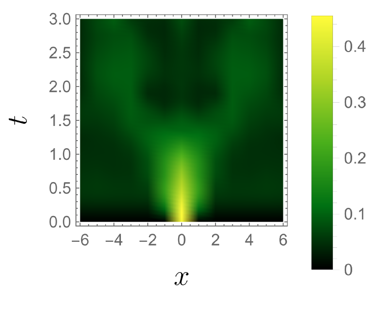
(b) $\gamma=0.3$

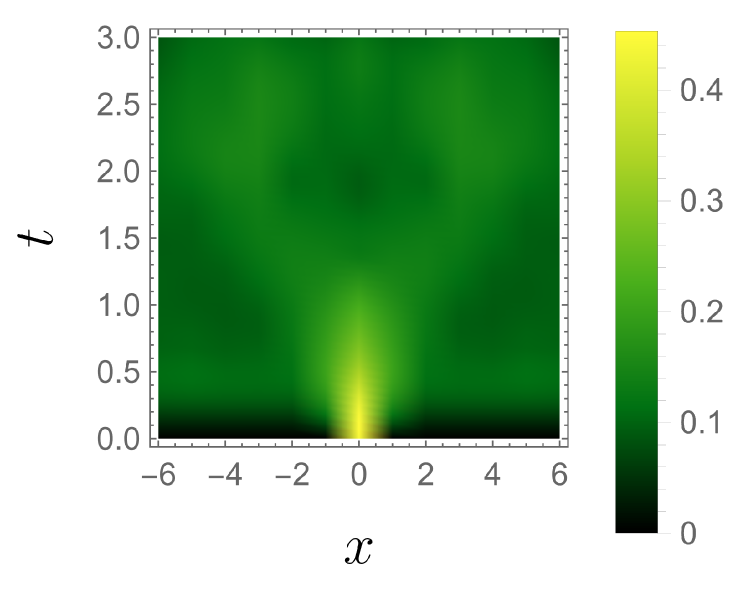
(c) $\gamma=0.6$

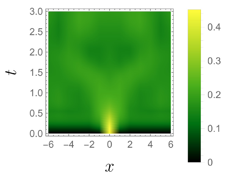
(d) $\gamma=0.9$

Figure 1: Plots of traditional $|\langle O_{A}(t),O_{B}(0)\rangle_{c}|$ for $A=0$ and $B=x$, averaged over $O_{A},O_{B}\in\{\sigma^{x},\sigma^{y},\sigma^{z}\}$, for the NH TFIM (Eq. 14), from an initial $|+^{n}\rangle$ state. As degree of non-Hermiticity $\gamma$ increases, the traditional CC ceases to demonstrate CC LR bound lightcones.

III.1 Schrödinger CC

As CCs are written in terms of correlators, we first extend the unequal-time disconnected correlator to NH systems. This can be done by interpreting operators as being applied at times $t^{\prime},t$ to some state $\rho$ undergoing normalized time evolution under a NH Hamiltonian, where the operators are excluded from the normalizing factor Sergi and Zloshchastiev (2015). With this interpretation, the correlator is

$$\begin{split}\langle O_{1}(t),O_{2}(t^{\prime})\rangle_{s}&\equiv\frac{\langle U^{\dagger}_{t}O_{1}U_{t-t^{\prime}}O_{2}U_{t^{\prime}}\rangle}{\langle U^{\dagger}_{t}U_{t}\rangle}\\ &=\frac{\langle O_{1}(t)\tilde{O}_{2}(t^{\prime})\rangle}{\langle I(t)\rangle}\end{split}$$ (16)

where $\tilde{O}(t)=U_{t}^{-1}OU_{t}$ is a modified notion of operator time evolution in NH systems, for which $U_{t}^{-1}\neq U_{t}^{\dagger}$. We refer to this as the Schrödinger correlator due to its motivation in terms of evolution of a state. This form has equivalence with the equal time correlator when $t=t^{\prime}$, in which case the denominator is simply the trace normalization of $\rho(t)$ in Eq. 12.

In extending this correlator to a CC, non-unitality of the $O(t)$ evolution requires additional caution. The standard definition equivalent to Eq. 5 is no longer zero for product evolutions on product states, as one would like a CC to be. Instead, we define

$$\begin{split}&\langle O_{1}(t),O_{2}(t^{\prime})\rangle_{sc}\\ &\equiv\langle O_{1}(t),O_{2}(t^{\prime})\rangle_{s}-\langle O_{1}(t),I(t^{\prime})\rangle_{s}\langle I(t),O_{2}(t^{\prime})\rangle_{s}\\ &=\frac{\langle O_{1}(t)\tilde{O}_{2}(t^{\prime})\rangle}{\langle I(t)\rangle}-\frac{\langle O_{1}(t)\rangle\langle I(t)\tilde{O}_{2}(t^{\prime})\rangle}{\langle I(t)\rangle^{2}}\end{split}$$ (17)

which recovers the desired locality behavior by explicitly subtracting out the product case. Despite this, the $O(t)$ evolution violates LR bounds, which means this CC can not be shown to obey the CC LR bound in general. In fact in the case $t^{\prime}=0$ it is equivalent to the traditional CC (Eq. 5), for which the lightcone breakdown is plotted in Fig. 1.

III.2 Metric CC

An alternative CC, which does recover LR bounds, can be derived from the metric formalism of NH systems Mostafazadeh (2003, 2002). For pseudo-Hermitian $H$ and Hermitian $\eta$ such that $\eta H=H^{\dagger}\eta$, consider the modified Hilbert space $\mathscr{H}_{\eta}$ with inner product $\langle\psi,\phi\rangle_{\eta}\equiv\langle\psi|\eta|\phi\rangle$. Within $\mathscr{H}_{\eta}$ the bra dual to ket $|\psi\rangle$ is $\langle\psi|\eta$, and so the representation of state $\rho$ in $\mathcal{L}(\mathscr{H}_{\eta})$ is Karuvade et al. (2022)

$$\sigma\equiv\frac{\rho\eta}{\langle\eta\rangle}$$ (18)

where $\langle\eta\rangle=\text{Tr}[\rho\eta]$ gives trace normalization in $\mathcal{L}(\mathscr{H}_{\eta})$.

When $\eta$ is invertible the modified adjoint in $\mathcal{L}(\mathscr{H}_{\eta})$, $O^{\#}\equiv\eta^{-1}O^{\dagger}\eta$, gives the canonical “Unitary” time evolution $U_{t}^{\#}OU_{t}=U_{t}^{-1}OU_{t}=\tilde{O}(t)$ for pseudo-Unitary $U=e^{-iHt}$. With this evolution and state $\sigma$, the standard unequal-time correlator in $\mathscr{H}_{\eta}$ is then

$$\langle O_{1}(t),O_{2}(t^{\prime})\rangle_{\eta}=\langle\tilde{O}_{1}(t)\tilde{O}_{2}(t^{\prime})\rangle_{\sigma}=\frac{\langle\eta\tilde{O}_{1}(t)\tilde{O}_{2}(t^{\prime})\rangle}{\langle\eta\rangle}$$ (19)

and the associated CC is

$$\begin{split}\langle O_{1}(t),O_{2}(t^{\prime})\rangle_{\eta c}&\equiv\\ \frac{\langle\eta\tilde{O}_{1}(t)\tilde{O}_{2}(t^{\prime})\rangle}{\langle\eta\rangle}&-\frac{\langle\eta\tilde{O}_{1}(t)\rangle\langle\eta\tilde{O}_{2}(t^{\prime})\rangle}{\langle\eta\rangle^{2}}\end{split}$$ (20)

We will refer to this as the Metric CC, and henceforth interpret it as a modified CC within the standard Hilbert space $\mathscr{H}$. Notice that since $U\rho\eta U^{-1}=U\rho U^{\dagger}\eta$, the equal-time Metric CC can be written in terms of time-evolved state $\rho(t)$ - this would not be the case if we were to, e.g., simply use the $\tilde{O}(t)$ evolution without $\eta$.

Note we are only guaranteed the existence of $\eta>0$, and thus non-degenerate $\langle\cdot,\cdot\rangle_{\eta}$, when $H$ is quasi-Hermitian. For indefinite $\eta$ this correlator is defined but less well motivated, and can diverge as $\langle\eta\rangle\rightarrow 0$.

An extension of both CCs to the $n$-partite case is discussed in Appendix B via a generalization of the CC generating function Tran et al. (2017); Sylvester (1975). Interestingly, the $n$-partite Metric CC takes a more natural form than the Schrödinger CC, stemming from the former’s role as standard CC in $\mathscr{H}_{\eta}$.

IV Connection to Entanglement

In this section we extend the relation between CCs and entanglement mentioned in Sec. II.2.1 by decomposing $\delta\rho\equiv\rho-\rho_{A}\otimes\rho_{B}$ as a sum of equal-time CCs between operators on subsystems $A$ and $B$. This allows extension of the CC LR bound to functions of $\delta\rho$, in particular $\|\delta\rho\|_{2}$ and mutual information $I(A;B)$. Additionally, we show how this decomposition extends to the Metric CC, where we find it holds for $\delta\sigma$ in general but $\delta\rho$ only when $A,B$ bipartition the entire system. Because of this difference, we note that the Metric CC LR bound does not extend to one on $\delta\rho$, as the bound requires some distance between $A$ and $B$ for information to propagate.

Let $\rho$ denote the state of the $AB$ (sub)system, which will be a reduced state when $A,B$ do not form a system bipartition. Consider operator Schmidt decomposition Zanardi (2001); Lupo et al. (2008); Aniello and Lupo (2009) of $\rho$,

$$\rho=\sum_{i=1}^{r}\lambda_{i}\ \Gamma_{A}^{i}\otimes\Gamma_{B}^{i}$$ (21)

where $r$ is the Schmidt rank of $\rho$, $\lambda_{i}=\langle\Gamma_{A}^{i{\dagger}}\otimes\Gamma_{B}^{i{\dagger}}\rangle\geq 0$, and $\{\Gamma_{X}^{i}\}_{i}$ are an orthonormal set $\text{Tr}[\Gamma_{X}^{i{\dagger}}\Gamma_{X}^{j}]=\delta_{ij}$ which can be extended to an operator basis on $X=A,B$. Let $C_{i}\equiv\langle\Gamma_{A}^{i{\dagger}},\Gamma_{B}^{i{\dagger}}\rangle_{c}$ be the traditional equal-time CC in Eq. 5, which can be equivalently taken with respect to the full system state or reduced state $\rho$. We may write

$$\begin{split}\rho&=\sum_{i=1}^{r}\left\langle\Gamma_{A}^{i{\dagger}}\otimes\Gamma_{B}^{i{\dagger}}\right\rangle\Gamma_{A}^{i}\otimes\Gamma_{B}^{i}\\ &=\sum_{i=1}^{r}\Big{(}\langle\Gamma_{A}^{i{\dagger}}\rangle\langle\Gamma_{B}^{i{\dagger}}\rangle+C_{i}\Big{)}\ \Gamma_{A}^{i}\otimes\Gamma_{B}^{i}\\ &=\rho_{A}\otimes\rho_{B}+\delta\rho\end{split}$$ (22)

with $\delta\rho\equiv\rho-\rho_{A}\otimes\rho_{B}=\sum_{i=1}^{r}C_{i}\ \Gamma_{A}^{i}\otimes\Gamma_{B}^{i}$. Then we find, for example,

$$\begin{split}\|\delta\rho\|_{2}^{2}&=\sum_{i,j=1}^{r}\overline{C}_{i}C_{j}\text{Tr}\left[\Gamma_{A}^{{\dagger}i}\Gamma_{A}^{j}\otimes\Gamma_{B}^{{\dagger}i}\Gamma_{B}^{j}\right]=\sum_{i=1}^{r}|C_{i}|^{2}\end{split}$$ (23)

For time evolved $\rho(t)$, we can use Eq. 8 to bound $|C_{i}|\leq\bar{c}\ e^{-\frac{L-2vt}{\chi^{\prime}}}$. Then by bounding $r\leq d_{\text{min}}^{2}$ for time-independent $d_{\text{min}}\equiv\text{min}(d_{A},d_{B})$, we find

$$\|\delta\rho(t)\|_{2}\leq\bar{c}\ d_{\text{min}}e^{-\frac{L-2vt}{\chi^{\prime}}}$$ (24)

The result is an operator-free LR bound on depending only on $\rho(t)$.

IV.1 Mutual Information Bound

As shown in Appendix C.1, when $\rho$ is full rank, the mutual information between $A,B$ can be bound in terms of $\delta\rho$ as

$$I(A;B)\leq\|\text{log}(k\rho)\|_{2}\|\delta\rho\|_{2}$$ (25)

where $k>0$ is a positive free parameter, which can be minimized to get the tightest bound. The logarithmic term can be shown to be constant, so when a CC LR bound is present, this allows placement of an LR bound on mutual information at time t:

$$\begin{split}I(A;B)(t)&\leq\|\text{log}(k\rho_{0})\|_{2}\|\delta\rho(t)\|_{2}\\ &\leq\tilde{c}\ d_{\text{min}}e^{-\frac{L-2vt}{\chi^{\prime}}}\end{split}$$ (26)

where $\tilde{c}=\overline{c}\|\text{log}(k\rho_{0})\|_{2}$ for initial state $\rho_{0}$. The full rank requirement on $\rho_{0}$ ensures that $\|\text{log}(k\rho_{0})\|_{2}$ is bounded. This condition is satisfied for generic $\rho_{0}$, for example by thermal subsystem states which can emerge even even in a closed overall system Popescu et al. (2006); D'Alessio et al. (2016); Borgonovi et al. (2016); Dymarsky et al. (2018).

As an example, consider thermal state $\rho_{0}=e^{-\beta H^{\prime}_{AB}}/Z$ under Hamiltonian $H^{\prime}_{AB}$, with $Z=\text{Tr}[e^{-\beta H^{\prime}_{AB}}]$. We can pick $k=Z$ so that $k\rho_{0}=e^{-\beta H^{\prime}_{AB}}$, and

$$\tilde{c}=\overline{c}\|\text{log}\left(e^{-\beta H^{\prime}_{AB}}\right)\|_{2}=\overline{c}\beta\|H^{\prime}_{AB}\|_{2}$$ (27)

Notice that $\|H^{\prime}_{AB}\|_{2}$ grows as as $O(d_{AB})$ rather than $O(d)$, making it bounded for fixed $|A|,|B|$ even in the thermodynamic limit. Such a case is illustrated in Fig. 2, where mutual information growth obeys a LR bound following a quench from an initial thermal state of $H^{\prime}_{AB}=-\sigma_{A}^{x}-\sigma_{B}^{x}$.

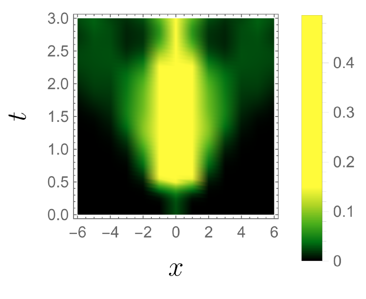
(a) $\gamma=0$

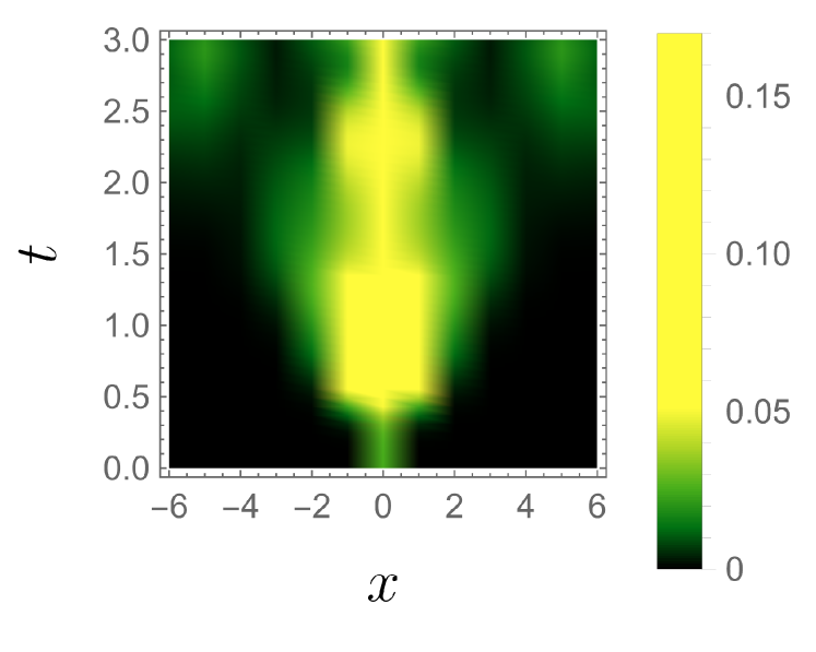
(b) $\gamma=0.3$

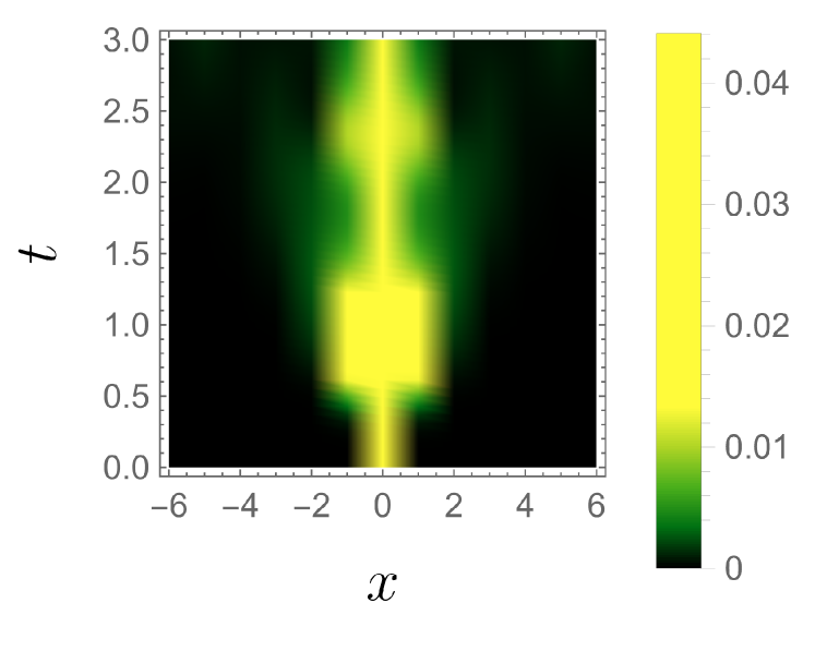
(c) $\gamma=0.6$

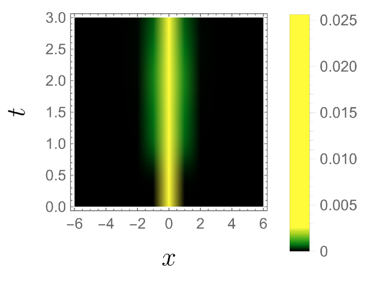
(d) $\gamma=0.9$

Figure 2: Plots of $I(A;B)$ for $A=0$ and $B=x$ for the NH TFIM (Eq. 14), from an initial Gibbs state at inverse temperature $\beta=3$ under Hamiltonian $-S_{x}$. $I(A;A)=H(A)$ at $A=x=0$ is included for completeness. One sees mutual information obeys a LR bound for all $\gamma$. However, as non-Hermiticity increases, the mutual information sharply decreases, especially for $|x|>1$.

IV.2 Entanglement in Non-Hermitian Systems

The aforementioned $\delta\rho$ decomposition is agnostic to time evolution, and so generalizes to NH systems. However, as the CC LR bound breaks down, Eq. 24 no longer holds in general. This motivates asking whether the Metric CC, which we will show does obey LR bounds, can be used instead to expand $\delta\rho$.

The result, as shown in Appendix C.3, is that when $A,B$ form a system bipartition and $\eta=\eta_{A}\otimes\eta_{B}$, $\delta\rho$ can be expanded as a linear combination of at most $4r$ Metric CCs. However when $A,B$ do not form a system bipartition, the presence of $\eta$ in the Metric CC prevents it from being written as a function of reduced state cleanly. That is, for tripartite system $ABC$, let $\rho$ now represent the overall state and $\rho_{AB}$ the state on $AB$. Even with $\eta=\eta_{AB}\otimes\eta_{C}$, we find

$$\begin{split}\langle\eta O_{A}O_{B}\rangle_{\rho}&=\text{Tr}[O_{A}O_{B}\text{Tr}_{C}[\rho\eta]]\\ &=\text{Tr}[\eta_{AB}O_{A}O_{B}\text{Tr}_{C}[\rho\eta_{C}]]\\ &\neq\langle\eta_{AB}O_{A}O_{B}\rangle_{\rho_{AB}}\end{split}$$ (28)

The same issue arises for CCs. Intuitively, $\eta_{C}$ modifies the entanglement properties of $\rho$ between the $A,B$ subsystems. Thus we cannot prove a LR bound on $\|\delta\rho(t)\|_{2}$ or mutual information in NH systems in the same way as for Hermitian ones, even though we still see one numerically in Fig. 2. This distinction has an interesting application, discussed in Sec. VI.1.

We can alternatively consider bounding $\delta\sigma(t)$. From Eq. 19, 20 we see that the Metric CC on state $\rho(t)$ is equivalent to a traditional CC on modified state $\sigma(t)$. This lets us use the decomposition in Eq. 22 to write $\delta\sigma(t)$ as a sum of Metric CCs, and so extend the Metric CC LR bound to a bound on $\|\delta\sigma(t)\|_{2}$. While $\sigma(t)$ has interpretation as a state in $\mathscr{H}_{\eta}$, its physical significance is unclear, so for now this bound is primarily of mathematical interest.

V LR Bounds of Modified CCs

We will now show the main result: that the Metric CC obeys a LR bound even in NH systems. We also find that the unequal-time Schrödinger CC obeys a LR bound when its initial state is a thermal state of the evolution Hamiltonian. Before that, notice that as any quasi-Hermitian $H$ will be Hermitian in modified Hilbert space $\mathscr{H}_{\eta}$, the generated dynamics can be shown to obey a LR bound in $\mathscr{H}_{\eta}$ in terms of modified operator norm $\|\cdot\|_{\eta}$. However the practical meaning of $\|\cdot\|_{\eta}$ is unclear, and as shown in Appendix. D, conversion to the traditional operator norm picks up overhead potentially exponential in $n$. This makes extending the LR bound this way of questionable utility. Instead, in this section we will show a LR bound on the Metric and Schrödinger CCs has no such overhead.

V.1 Metric CC

When $H$ is quasi-Hermitian under product $\eta$ and sufficiently local, a LR bounds holds for the Metric CC. This can be shown by decomposing $H=SH_{0}S^{-1}$ for Hermitian $H_{0}$ and $S=\eta^{-1/2}$. Then $U_{t}=SV_{t}S^{-1}$ for $V_{t}=e^{-iH_{0}t}$, and one can rewrite the Metric correlator in terms of Unitary evolutions on modified state and operators:

$$\langle O_{A}(t),O_{B}(t^{\prime})\rangle_{\eta}=\langle V_{t}^{\dagger}\hat{O}_{A}V_{t-t^{\prime}}\hat{O}_{B}V_{t^{\prime}}\rangle_{\hat{\sigma}}$$ (29)

where $\hat{O}_{X}\equiv S^{-1}O_{X}S$ and $\hat{\sigma}\equiv S^{-1}\sigma S=\langle\eta\rangle_{\rho}^{-1}S^{-1}\rho S^{-1}$. This can be interpreted as using the map $S:\mathscr{H}\rightarrow\mathscr{H}_{\eta}$ to rewrite evolution of operators on $\mathscr{H}_{\eta}$ in terms of evolution of operators on $\mathscr{H}$. For product $S$ decomposable as $S=S_{X}\otimes S_{\overline{X}}$ the similarity transform of operators is locality-preserving: $\hat{O}_{X}=S^{-1}_{X}O_{X}S_{X}$. In this case the entire Metric CC may be written as a traditional CC with Unitary evolution $\hat{O}(t)\equiv V^{\dagger}_{t}\hat{O}V_{t}$:

$$\begin{split}&\langle O_{A}(t),O_{B}(t^{\prime})\rangle_{\eta c}\\ &=\langle\hat{O}_{A}(t)\hat{O}_{B}(t^{\prime})\rangle_{\hat{\sigma}}-\langle\hat{O}_{A}(t)\rangle_{\sigma}\langle\hat{O}_{B}(t^{\prime})\rangle_{\hat{\sigma}}\end{split}$$ (30)

Thus, we can directly apply locality results on traditional CCs with Unitary evolution, such as LR bounds and exponential clustering Tran et al. (2017); Bravyi et al. (2006); Nachtergaele and Sims (2006a). Using the bound in Eq. 9, we find

$$|\langle\hat{O}_{A}(t),\hat{O}_{B}(t^{\prime})\rangle_{\eta c}|\leq\bar{c}\ \|\hat{O}_{A}\|\|\hat{O}_{B}\|e^{-\frac{L-v(t+t^{\prime})}{\chi^{\prime}}}$$ (31)

with $\|\hat{O}_{X}\|\leq\|S_{X}\|\|S^{-1}_{X}\|$ for product $S$, taking $\|O_{X}\|\leq 1$ without loss of generality. $\|S_{X}\|,\|S_{X}^{-1}\|$ can grow as $O(d_{X})$, but will be finite for fixed $|X|$ even in the thermodynamic limit.

This bound requires that $H_{0}$ be composed of sufficiently local terms as in the original LR bound, and that $\hat{\sigma}$ exhibit finite correlation length. The former follows from locality of $H$, as when $S$ is a tensor product over subsystems of fixed locality, such a single qubits, the locality properties of $H$ and $H_{0}$ will be equivalent. That is, let $H=\sum_{R}h_{R}$ and take $S=\otimes_{Q}S_{Q}$ for $R,Q$ of fixed locality. With $R^{\prime}\equiv\cup_{Q\cap R\neq\varnothing}Q^{\prime}$, we can write $S=S_{R^{\prime}}\otimes S_{\overline{R^{\prime}}}$ for each $R^{\prime}$. Then

$$H_{0}=S^{-1}(\sum_{R}h_{R})S=\sum_{R}S^{-1}_{R^{\prime}}h_{R}S_{R^{\prime}}$$ (32)

which satisfies the conditions for a LR bound due to fixed locality of $R^{\prime}$. For example when $Q$ are single qubits, $R^{\prime}=R$ simply.

Finite correlation length of $\hat{\sigma}$ is similarly motivated, though difficult to prove in general due to lack of cancellation. In the case that $\rho$ is the ground state of gapped $H$, $\hat{\sigma}$ is the ground state of the gapped isospectral $H_{0}$, guaranteeing finite correlation length Nachtergaele and Sims (2006b).

An example quasi-Hermitian system with product Metric is the NH TFIM Matsumoto et al. (2020); Barch et al. (2023). For this system we can pick $S$ as in Eq. 15, for which $\|S_{X}\|=\|S^{-1}_{X}\|=e^{|X|/2}$. This choice results in the lightcone structure in Fig. 3, indicative of the Metric CC LR bound.

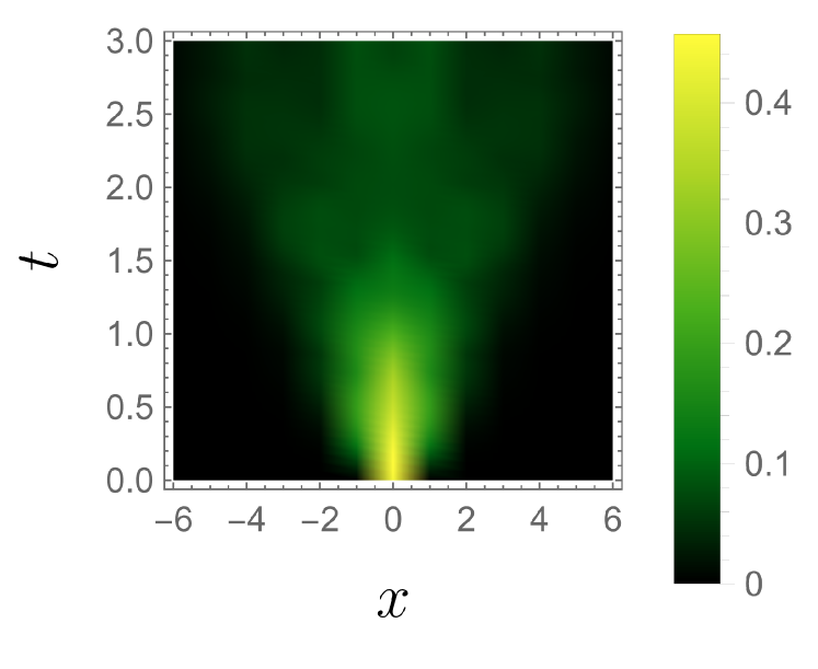
(a) $\gamma=0$

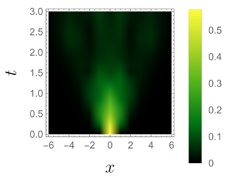
(b) $\gamma=0.3$

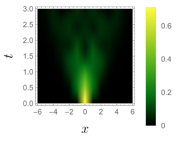
(c) $\gamma=0.6$

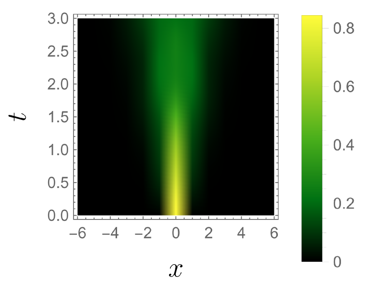
(d) $\gamma=0.9$

Figure 3: Plots of $\langle O_{A}(t),O_{B}(0)\rangle_{\eta c}$ for $A=0$ and $B=x$, summed over $O_{A},O_{B}\in\{\sigma^{x},\sigma^{y},\sigma^{z}\}$. The lightcone structure is preserved as $\gamma$ increases, unlike for the Schrödinger CC. Narrowing of the lightcone can be attributed to a decreased LR velocity, as for $\gamma\approx 1$ the Hamiltonian transitions from volume-law to area-law entanglement generation Barch et al. (2023)

V.2 Schrödinger CC

The Schrödinger correlator can be decomposed similarly to Eq. 29, yielding

$$\langle O_{A}(t),O_{B}(t^{\prime})\rangle_{s}=\frac{\langle\eta\rangle\langle V_{t}^{\dagger}(SO_{A}S)V_{t-t^{\prime}}\hat{O}_{B}V_{t^{\prime}}\rangle_{\hat{\sigma}}}{\langle I(t)\rangle}$$ (33)

Unlike $\hat{O}_{A}$, $SO_{A}S$ can be generally nonlocal, preventing placement of a LR bound on the Schrödinger CC in general. The exception is that when $\rho$ is a thermal state of $H$, the Schrödinger correlator is time invariant like in the Hermitian case:

$$\langle O_{A}(t)\tilde{O}_{B}(t^{\prime})\rangle_{s}=\langle O_{A}(0)\tilde{O}_{B}(t-t^{\prime})\rangle_{s}$$ (34)

In this case the time dependence of the Schrödinger CC is limited to $\tilde{O}_{B}(t-t^{\prime})$, and the CC can be decomposed in terms of $\hat{O}_{A}$, $\hat{O}_{B}$ as

$$\begin{split}\langle O_{A}(t),O_{B}(t^{\prime})\rangle_{sc}&=\langle O_{A}(0),O_{B}(t-t^{\prime})\rangle_{sc}\\ &=\langle\hat{O}_{A},\hat{O}_{B}(t^{\prime}-t)\rangle_{c,\hat{\rho}}\end{split}$$ (35)

For $\hat{\rho}=S^{-1}\rho S$. Then if one assumes that $\hat{\rho}$ has finite correlation length, the CC LR bound for Unitary evolution applies:

$$\left|\langle O_{A}(t),O_{B}(t^{\prime})\rangle_{sc}\right|\leq\bar{c}\ \|\hat{O}_{A}\|\|\hat{O}_{B}\|e^{-\frac{L-v|t^{\prime}-t|}{\chi^{\prime}}}$$ (36)

Unfortunately this bound is only nontrivial for the unequal time CC, limiting its application towards describing properties of the state such as entanglement. Finite correlation length of $\hat{\rho}$ is also harder to motivate than for $\hat{\sigma}$, as $\hat{\rho}$ is not a proper state.

V.3 Generalization

Quasi-Hermiticity of $H$ under product $\eta$ is not strictly necessary for existence of a LR bound on the Metric CC; a bound on $\|\tilde{O}_{X}(t)\|=\|U_{t}^{-1}O_{X}U_{t}\|$ is sufficient. Given existence of such a bound, one can retrace the steps in Sec. II.2 to derive an LR bound on both the Metric CC and the thermal state Schrödinger CC, without relying on a decomposition of $U_{t}$. The presence of such an LR bound is well motivated, since the breakdown of LR bounds for $O(t)$ in Sec. II.1 does not occur for the $\tilde{O}(t)$ evolution:

$$\dot{\tilde{O}}_{A}\big{|}_{t=0} =i[H_{\mathrm{eff}},\tilde{O}_{A}]=i\sum_{R\cap A\neq\varnothing}[H_{R}+i\Gamma_{R},\tilde{O}_{A}]$$

However while we see evidence for such a LR bound in Fig. 4, a general analytic proof is not evident, and even in the quasi-Hermitian case of Appendix D the bound incurs overhead potentially exponential in system size.

VI Applications

Here we discuss two more practical results: how the previous Metric CC LR bound can place a necessary condition of the set of NH Hamiltonians capable of generating long-range entangled states, and how traditional and metric CCs may be measured as a series of POVMs.

VI.1 Preparing Long-range Entangled States

Limits on entanglement growth under local Hamiltonians has motivated interest in non-local entanglement protocols such as gate teleportation and entanglement swapping, which augment Unitary evolution with measurement and classical communication Nielsen and Chuang (2010). NH Hamiltonians provide an alternative method of generating non-local entanglement, where classical communication is replaced by postselection. The Metric CC LR bound restricts this long range entangling power, but by finding cases where the bound is trivially satisfied, we can derive a necessary condition on the class of quasi-Hermitian Hamiltonians capable of generating long range entangled states in short times.

Consider first Hermitian systems, where the CC LR bound (Eq. 8) can be solved for $t$ to lower bound the time needed to generate a given state. For example, the $n$-qubit GHZ state has $\langle\sigma_{1}^{z},\sigma_{n}^{z}\rangle_{c}=1$, while the CC LR bound states that $|\langle\sigma^{z}_{1}(t),\sigma^{z}_{n}(t)\rangle_{c}|\leq\overline{c}\ e^{-\frac{n-2vt}{\chi^{\prime}}}$. Thus as $n\rightarrow\infty$, the time needed to generate the GHZ state an initial state with finite correlation length becomes infinite.

In quasi-Hermitian systems, this logic can be extended to the Metric CC. Solving the Metric CC LR bound in Eq. 31 for $t=t^{\prime}$ yields

$$t\geq\frac{\chi^{\prime}}{2v}\text{log}\left(\frac{|\langle\hat{O}_{A}(t),\hat{O}_{B}(t^{\prime})\rangle_{\eta c}|}{\bar{c}\ \|\hat{O}_{A}\|\|\hat{O}_{B}\|}\right)+\frac{L}{2v}$$ (37)

in particular as $L\rightarrow\infty$, $t\rightarrow\infty$. The exception is that when the Metric CC is zero for all $t$, the LR bound is trivially satisfied and no longer restricts $t$. As we now show, this can occur even for entangled $\rho$.

As mentioned at the end of Sec. IV, the Metric CC quantifies the entanglement of $\sigma$, rather than $\rho$ itself. For a tripartite system $ABC$ the two can be different even for product $\eta$, and if $\sigma_{AB}=\text{Tr}_{C}[\sigma]=\langle\eta\rangle^{-1}\text{Tr}_{C}[\rho\eta]$ is product between $A$ and $B$, the Metric CC will be zero for all operator pairs $O_{A},O_{B}$. In particular if $\sigma(t)_{AB}=\langle\eta\rangle^{-1}\text{Tr}_{C}[\rho(t)\eta]$ is product for all $t$, the Metric CC LR bound will become trivial.

For given $\rho$ and $H$, and $t\in\mathbb{R}$, consider the two sets

$$\begin{split}\mathbb{F}_{\rho(t)}&=\{\eta\ :\ \sigma(t)_{AB}\ \text{product on }A|B\}\\ \mathbb{G}_{H}&=\{\eta\ :\ H^{\dagger}\eta=\eta H^{\dagger},\eta\text{ product on }A|B|C\}\end{split}$$ (38)

For $H,\rho_{0}=\rho(0)$ with $\mathbb{G}_{H}\subseteq\cap_{t}\mathbb{F}_{\rho(t)}$, the Metric CC LR bound is trivial for all $t$ and no longer restricts the entangling power of $H$. Thus if one wishes to generate long range entanglement under quasi-Hermitian Hamiltonians, it is this set of $H,\rho_{0}$ that must be considered. An example system where $\sigma(t)_{AB}$ stays product while $H$ entangles $\rho(t)$ is provided in Appendix E.

VI.2 Measurement as POVM

NH time evolutions on states can be generated by combining Unitary evolution with weak measurement and postselectionAshida et al. (2020), or by changing system metric by applying $S$ as a positive operator valued measurement (POVM) Karuvade et al. (2022). However, unequal-time correlators introduce ambiguity from the interaction between applied operators and state normalization, such as occurs in Refs. Sergi and Zloshchastiev (2015); Barch et al. (2023), and in operator time evolution itself. Though the CCs described in this paper are written in terms of operator time evolution, here we show how they can be measured as the joint success probability of a series of POVMs and state evolutions, where the state evolutions need not be normalized, resolving ambiguity. An alternative approach is seen in Ref. Matsumoto et al. (2022), where the Metric correlator on a thermal state is mapped to a standard correlator on an extended Hermitian system via projective measurements.

Application of operator $O_{i}$ with $\|O_{i}\|\leq 1$ via POVM to an initial pure state $|\psi\rangle$ succeeds with probability $P(O_{i})=\|O_{i}|\psi\rangle\|^{2}$. Similarly, evolving $|\psi\rangle$ under well-behaved $U_{t}$ generated by a NH Hamiltonian, e.g. as generated by weak measurement conditioned on certain outcomes, succeeds with probability $P(U_{t})=\|U_{t}|\psi\rangle\|^{2}$. To see this, one could imagine a Trotter expansion of $U_{t}$ alternating Unitary evolution with near-identity POVMs. By well-behaved $U_{t}$, we mean that success probability must be non-increasing over time, which follows from assuming success at each time step is independent. This then imposes a condition on NH Hamiltonian $H$. Let $H=H_{0}-i\Gamma$ for Hermitian $H_{0},\Gamma$, then

$$\begin{split}\frac{d}{dt}\||\psi(t)\rangle\|^{2}&=i\langle\psi(t)|H^{\dagger}-H|\psi(t)\rangle\\ &=-2\langle\psi(t)|\Gamma|\psi(t)\rangle\end{split}$$ (39)

so success probability $\||\psi(t)\rangle\|^{2}$ is nonincreasing regardless of $|\psi\rangle$ when $\Gamma\geq 0$. This occurs naturally for $H$ coming from no-jump Lindblad evolution (Eq. 11) and can be equivalent to pseudo-Hermitian evolution up to a constant shift in $\Gamma$. Interestingly even when the minimum eigenvalue of $\Gamma$ is zero, $\|U_{t}\|$ and thus $\||\psi(t)\rangle\|^{2}$ may still exhibit exponential decay owing to $H_{0}$ mixing eigenspaces of $\Gamma$.

Using Bayes rule, the probability of applying a pair of operators via separate POVMs (or non-Unitary evolutions) can be written cleanly as

$$\begin{split}P(O_{A},O_{B})&=P(O_{A}|O_{B})\cdot P(O_{B})\\ &=\left\|O_{A}\frac{O_{B}|\psi\rangle}{\|O_{B}|\psi\rangle\|}\right\|^{2}\cdot\|O_{B}|\psi\rangle\|^{2}\\ &=\|O_{A}O_{B}|\psi\rangle\|^{2}\\ &=P(O_{A}O_{B})\end{split}$$ (40)

Treating measurement of $\Pi_{\psi}=|\psi\rangle\langle\psi|$ similarly, we find, e.g.,

$$\begin{split}P(\Pi_{\psi},U_{t}^{\dagger},O_{A},U_{t},O_{B})&=\|\Pi_{\psi}U_{t}^{\dagger}O_{A}U_{t}O_{B}|\psi\rangle\|^{2}\\ &=|\langle\psi|U_{t}^{\dagger}O_{A}U_{t}O_{B}|\psi\rangle|^{2}\end{split}$$ (41)

This extends similarly to all other expectation values used in this paper, and all CCs can be calculated in terms of success probabilities, each of which can be measured independantly. Decay of success probability with time and number of operations can make the process take exponentially many measurements to accurately estimate expectation values, but by accounting for this we have escaped the hidden costs inherent in the usual postselection. In the case of quasi-Hermitian evolution, $S$ and $S^{-1}$ can be applied independently as in Ref. Karuvade et al. (2022), or absorbed into existing operators applied as POVMs, leaving all necessary time evolution Unitary.

VII Discussion

While non-Hermitian quantum systems have a long history, their study under the lens of quantum information is relatively new, leaving much room for generalization of existing methods and bounds. Interaction between the metric formalism of non-Hermitian systems and information theoretic quantities is especially interesting, as the formalism provides a unified way to study a large class of non-Hermitian systems of interest. Here we used this approach to extend the well-studied LR bound to connected correlators on non-Hermitian systems. This is significant as the usual LR bound was previously shown to break down in these systems, and even when applied to the unital $\tilde{O}(t)$ evolution picks up exponential overhead not present in the connected correlator LR bound.

The connected correlator LR bound here discussed promises insight into many questions of entanglement in non-Hermitian systems, such as the recently popular topic of measurement-induced phase transitions, a phenomena describable by non-Hermitian Hamiltonians Li et al. (2018); Skinner et al. (2019); Chan et al. (2019); Li et al. (2019); Gullans and Huse (2020); Choi et al. (2020); Ippoliti et al. (2021); Agarwal et al. (2023), or the topic of non-Hermitian quantum chaos Efetov (1997); Chalker and Wang (1997); Fyodorov et al. (1997, 1998); Fyodorov and Sommers (2003); Barch et al. (2023). As seen in Fig. 3, the Metric connected correlator reveals a sharp drop in LR velocity for the imaginary Transverse-Field Ising Model near critical measurement strength $\gamma\approx 1$, seemingly detecting the Hamiltonian’s phase transition from chaotic to integrable that occurs at this point Gopalakrishnan and Gullans (2021); Barch et al. (2023). Furthermore the Metric connected correlator diverges at exceptional points, where $\eta$ becomes indefinite, allowing it to detect measurement induced criticality.

The LR bounds shown on entanglement and mutual information in Sec. IV are novel in that they give operator-free bounds on information scrambling. In addition, they have implications towards the construction of efficient MPS representation of $\rho$ in Hermitian systems, and thus towards simulability and quantum computational complexity of these systems Preskill (2012). The extension to bounding entanglement of $\sigma$ in non-Hermitian systems means these systems, traditionally believed more difficult to simulate due to LR bound violation, may be simulable via MPS representation of $\sigma$ rather than $\rho$. Utility of using the entanglement of $\sigma$ to bound that of $\rho$ remains a topic for further study, as even in the bipartite case the bound has overhead proportional to $\|\eta\|$, which can grow exponentially.

Finally, it is worth noting that any evolution with measurement and classical action can be written as an ensemble of postselected quantum evolutions, potentially allowing results from non-Hermitian systems to generalize to this unconditional yet non-Markovian case. In particular, while Sec. VI.1 places restrictions on long range entanglement generation under non-Hermitian evolution, it may be possible to extend this to bound generation of long range entanglement via classical communication, e.g. as used in entanglement swapping and teleportation.

VIII Acknowledgements

This research was partially supported by the ARO MURI grant W911NF-22-S-0007. B.B. would like to thank Namit Anand, Daniel Lidar, and Paolo Zanardi for insightful discussions during the writing of this paper.

Appendix A LR bound on unequal-time CCs

This section extends the proof of LR bounds for equal-time CCs in Eq. 8 and Ref. Bravyi et al. (2006) to the unequal-time case. Given

$$\begin{split}&\left|\langle O_{A}(t),O_{B}(t^{\prime})\rangle_{c}\right|\\ &\leq\left|\langle O_{A}^{l}(t),O_{B}^{l}(t^{\prime})\rangle_{c}\right|+c|A|e^{\frac{l-vt}{\xi}}+c|B|e^{\frac{l^{\prime}-vt^{\prime}}{\xi}}\\ &\leq\tilde{c}\ e^{-\frac{L-l-l^{\prime}}{\chi}}+c|A|e^{\frac{l-vt}{\xi}}+c|B|e^{\frac{l^{\prime}-vt^{\prime}}{\xi}}\end{split}$$ (A.1)

we can pick the optimal $l=(\xi L+\chi vt+\xi v(t-t^{\prime}))/\chi^{\prime}$ and $l^{\prime}=(\xi L+\chi vt^{\prime}+\xi v(t^{\prime}-t))/\chi^{\prime}$. Plugging this in yields Eq. 9. This bound can be extended to the $n$-partite $n$-time case following the steps of Ref. Tran et al. (2017), but the interplay of multiple distances and times makes the results quite cumbersome.

Appendix B $n$-partite extension of CCs

The CCs in Sec. III extend to the $n$-partite case via a generalization of the generating function in Eq. B.2 and Refs. Sylvester (1975); Tran et al. (2017) to the unequal-time case. Recall that the standard CC can be extended to $n$ operators by writing it as a sum over partitions $P$ of the set $\{1,...,n\}$ Sylvester (1975); Tran et al. (2017)

$$\langle O_{1},...,O_{n}\rangle_{c}=\sum_{P}g(|P|)\prod_{p\in P}\left\langle\prod_{i\in p}O_{i}\right\rangle$$ (B.1)

for $g(x+1)=(-1)^{x}x!$. This can further be written in terms of a generating function as

$$\langle O_{1},...,O_{n}\rangle_{c}\equiv\frac{\partial^{n}}{\partial\lambda_{1}...\partial\lambda_{n}}\text{ln}\left\langle e^{\sum_{i}\lambda_{i}O_{i}}\right\rangle\bigg{|}_{\vec{\lambda}=0}$$ (B.2)

For Hermitian systems this can simply be written in terms of time evolved operators as e.g. $O_{i}\rightarrow O_{i}(t_{i})$. However in NH systems the Heisenberg picture becomes ambiguous, so here we reconstruct the generating function in terms of evolution of states.

B.1 General form of CC generating function

Consider $n$ copies of the system with some $O_{i}$ acting on the $i^{th}$ copy. Define the cyclic permutation over system copies $P=\prod_{i=2}^{n}\mathbb{S}_{i-1,i}$ for SWAP operator $\mathbb{S}$, and extended state $\rho^{\prime}=P(\rho\otimes I^{\otimes n-1})$ (akin to as written in Ref. Anand and Zanardi (2022)).

For time-evolution channel $\mathcal{E}_{\vec{t}}=\otimes_{i}\mathcal{E}_{t_{i}}$, and $\langle\vec{O}(\vec{t})\rangle_{c}\equiv\langle O_{1}(t_{1}),...,O_{n}(t_{n})\rangle_{c}$, a general generating function and $n$-partite CC are given by

$$\begin{split}\langle\vec{O}(\vec{t})\rangle_{c}&=\frac{\partial^{n}}{\partial\lambda_{1}...\partial\lambda_{n}}\text{ln}\Big{\langle}\otimes_{i}e^{\lambda_{i}O_{i}}\Big{\rangle}_{\mathcal{E}_{\vec{t}}(\rho^{\prime})}\bigg{|}_{\vec{\lambda}=0}\\ &=\frac{\partial^{n}}{\partial\lambda_{1}...\partial\lambda_{n}}\text{ln}\left\langle\otimes_{i}\mathcal{E}^{\dagger}_{t_{i}}\left(e^{\lambda_{i}O_{i}}\right)\right\rangle_{\rho^{\prime}}\bigg{|}_{\vec{\lambda}=0}\\ &=\sum_{P}\frac{g\big{(}|P|\big{)}}{\big{\langle}\prod_{i}\mathcal{E}^{\dagger}_{t_{i}}(I)\big{\rangle}^{|P|}}\prod_{p\in P}\Big{\langle}\prod_{i}\mathcal{E}^{\dagger}_{t_{i}}(O_{i}^{p_{i}})\Big{\rangle}\end{split}$$ (B.3)

for indicator variables $p_{i}\in\{0,1\}$ so that $O_{i}^{p_{i}}=O_{i}$ iff $i\in p$ and $O_{i}^{p_{i}}=I$ otherwise. In the case of Unitary (or any trace-preserving) $\mathcal{E}$, the adjoint channel $\mathcal{E}^{\dagger}$ is unital and this reduces to the usual form in Eq. B.1 with $O_{i}\rightarrow O_{i}(t_{i})$. Eq. B.3 is used to derive the generating functions for the Schrödinger and Metric CCs (Eq. B.6 and Eq. B.7). For the Shrodinger CC we take $\mathcal{E}_{t_{1}}(\cdot)=U_{t_{1}}\cdot U_{t_{1}}^{\dagger}=U_{t_{1}}\cdot\eta U_{t_{1}}^{-1}\eta^{-1}$ and $\mathcal{E}_{t_{i}}(\cdot)=U_{t_{i}}\cdot U_{t_{i}}^{-1}$ for $i\neq 1$, while for the Metric CC we use the $\mathcal{E}_{t_{i}}=U_{t_{1}}\cdot U_{t_{i}}^{-1}\ \forall i$, with $\rho\rightarrow\sigma=\frac{\rho\eta}{\langle\eta\rangle}$.

The proof of vanishing CCs for product states in Ref. Tran et al. (2017) holds for this general form as well in the case of product time evolution. The $n$-partite CC derived here is also inherently normalized even when $\rho$ is not, making trace normalization of $\rho^{\prime}(\vec{t}\ )$ optional when extending to non-trace-preserving time evolution.

B.2 $n$-partite Schrödinger and Metric CCs

We can use this general form to construct generating functions for the $n$-partite Schrödinger and Metric CCs, yielding forms guaranteed to be zero for product evolutions on product states. These generating functions can be written in terms of a modified initial state $\sigma^{\prime}=P(\rho\eta\otimes I^{\otimes n-1})$ and time evolution $\tilde{\sigma}^{\prime}(\vec{t})=U_{\vec{t}}\sigma^{\prime}U_{\vec{t}}^{-1}$. With this, we get the generating functions

$$\langle\vec{O}(\vec{t})\rangle_{sc} =\frac{\partial^{n}}{\partial\lambda_{1}...\partial\lambda_{n}}\text{ln}\Big{\langle}\eta^{-1}_{1}\left(\otimes_{i}e^{\lambda_{i}O_{i}}\right)\Big{\rangle}_{\tilde{\sigma}^{\prime}(\vec{t})}\bigg{|}_{\vec{\lambda}=0}$$ (B.4)

and

$$\langle\vec{O}(\vec{t})\rangle_{\eta c} =\frac{\partial^{n}}{\partial\lambda_{1}...\partial\lambda_{n}}\text{ln}\Big{\langle}\otimes_{i}e^{\lambda_{i}O_{i}}\Big{\rangle}_{\tilde{\sigma}^{\prime}(\vec{t})}\bigg{|}_{\vec{\lambda}=0}$$ (B.5)

for the $n$-partite Schrödinger and Metric CCs, respectively, where $\eta^{-1}_{1}\equiv\eta^{-1}\otimes I^{\otimes n-1}$. Writing the equal-time $n$-partite Metric CC in this form allows extension of the LR bound, shown for the two-partite Metric CC in Sec. V, to the $n$-partite case via the results of Ref. Tran et al. (2017).

From the generating functions we derive that the explicit form of the $n$-partite Schrödinger CC is

$$\langle\vec{O}(\vec{t})\rangle_{\eta c}=\sum_{P}\frac{g\big{(}|P|\big{)}}{\langle I(t_{1})\rangle^{|P|}}\prod_{p\in P}\Big{\langle}O_{1}^{p_{1}}(t_{1})\prod_{i\in p,i\neq 1}\tilde{O}_{i}(t_{i})\Big{\rangle}$$ (B.6)

for indicator variable $p_{1}$ such that $O_{1}^{p_{1}}=O_{1}$ iff $1\in p$ and $O_{1}^{p_{1}}=I$ otherwise. For the Metric CC it is

$$\langle\vec{O}(\vec{t})\rangle_{\eta c}=\sum_{P}\frac{g\big{(}|P|\big{)}}{\langle\eta\rangle^{|P|}}\prod_{p\in P}\Big{\langle}\eta\prod_{i\in p}\tilde{O}_{i}(t_{i})\Big{\rangle}$$ (B.7)

Appendix C Entanglement, Information, and CCs

In this section we show that when $\rho$ is full rank, mutual information can be upper bounded in terms of $\|\delta\rho\|_{2}$ for $\delta\rho=\rho-\rho_{A}\otimes\rho_{B}$, and when applicable in terms of a LR bound. Additionally, we discuss two extensions of the decomposition of $\delta\rho$ in Sec. IV, the first to an arbitrary operator basis and the second to NH systems.

C.1 Bounding Mutual Information

Here we show that mutual information $I(A;B)$ can be upper bounded in terms of $\|\delta\rho\|_{2}$. Using the CC bound on $\|\delta\rho\|_{2}$ in Eq. 23, one can then bound it in terms of a sum of CCs, and when dynamics are sufficiently local in terms of a LR bound. The requirement is that the reduced state $\rho$ on the two subsystems $A,B$ is full rank so that $\text{log}(\rho)$ is bounded from below. This condition is generically satisfied, for example by thermal states which can emerge in subsystems of even a closed overall system Popescu et al. (2006); D'Alessio et al. (2016); Borgonovi et al. (2016); Dymarsky et al. (2018).

Let $H(X)=-\text{Tr}[\rho_{X}\text{log}(\rho_{X})]$ denote entropy on the $X$ subsystem. Mutual information is defined as

$$I(A;B)=H(A)+H(B)-H(AB)$$ (C.1)

$$=\text{Tr}[\rho\text{log}(\rho)]-\text{Tr}[\rho_{A}\otimes\rho_{B}\text{log}(\rho_{A}\otimes\rho_{B})]$$

$$=\text{Tr}[\rho_{A}\otimes\rho_{B}(\text{log}(\rho)-\text{log}(\rho_{A}\otimes\rho_{B}))]+\text{Tr}[\delta\rho\text{log}(\rho)]$$

$$=\text{Tr}[\delta\rho\text{log}(\rho)]-D(\rho_{A}\otimes\rho_{B}\|\rho)$$

Where in the second line we use $\text{Tr}[\rho_{A}\otimes\rho_{B}\text{log}(\rho_{A}\otimes\rho_{B})]=\text{Tr}[\rho_{A}\text{log}(\rho_{A})]+\text{Tr}[\rho_{B}\text{log}(\rho_{B})]=-H(A)-H(B)$. The second term in the final line is $\leq 0$ owing to non-negativity of relative entropy $D$. For the first term note that since $\text{Tr}[\delta\rho]=0$ we can shift $\text{log}(\rho)\rightarrow\text{log}(k\rho)=\text{log}(\rho)+\text{log}(k)\mathbb{I}$ for $k>0$ without changing the overall quantity. Then using Hödler’s inequality,

$$\begin{split}I(A;B)&\leq\text{Tr}[\delta\rho\text{log}(k\rho)]\\ &\leq\|\delta\rho\|_{2}\|\text{log}(k\rho)\|_{2}\end{split}$$ (C.2)

Interestingly, as $\text{log}(U\rho U^{\dagger})=U\text{log}(\rho)U^{\dagger}$ and the 2-norm is invariant under unitary rotations, $\|\text{log}(k\rho)\|_{2}$ is time-independent under unitary evolution and may be written in terms of initial state $\rho_{0}$. Thus from the LR bound on $\|\delta\rho(t)\|_{2}$ in Eq. 24, we find a LR bound on mutual information

$$\begin{split}I(A;B)(t)&\leq\|\delta\rho(t)\|_{2}\|\text{log}(k\rho_{0})\|_{2}\\ &\leq d_{\text{min}}\overline{c}\ \|\text{log}(k\rho_{0})\|_{2}\ e^{-\frac{L-2vt}{\chi^{\prime}}}\end{split}$$ (C.3)

C.2 Alternative choice of basis

Given that the Schmidt decomposition can be hard to calculate, the bound in Sec. IV can also be found using an arbitrary orthonormal product basis for $AB$, $\{\Gamma_{A}^{i},\Gamma_{B}^{j}\}$. Let $C_{ij}=\langle\Gamma_{A}^{i{\dagger}},\Gamma_{B}^{j{\dagger}}\rangle_{c}$ be the traditional equal-time CC. Then

$$\begin{split}\rho&=\sum_{ij}\left\langle\Gamma_{A}^{i{\dagger}}\otimes\Gamma_{B}^{j{\dagger}}\right\rangle\Gamma_{A}^{i}\otimes\Gamma_{B}^{j}\\ &=\sum_{ij}\Big{(}\langle\Gamma_{A}^{i{\dagger}}\rangle\langle\Gamma_{B}^{j{\dagger}}\rangle+C_{ij}\Big{)}\Gamma_{A}^{i}\otimes\Gamma_{B}^{j}\\ &=\rho_{A}\otimes\rho_{B}+\delta\rho\end{split}$$ (C.4)

for $\delta\rho=\sum_{ij}C_{ij}\ \Gamma_{A}^{i}\otimes\Gamma_{B}^{j}$.

C.3 Metric CC

Recall that the Metric CC on $\rho$ is equivalent to traditional CC on modified state $\sigma$ (Eq. 19), or on modified state $\hat{\sigma}$ and operators $\hat{O}_{X}$ (Eq. 30). This allows decomposition of $\delta\sigma$ and $\delta\hat{\sigma}$ in terms of a sum of Metric CCs on $\rho$. While $\delta\sigma$ and $\delta\hat{\sigma}$ have value in the metric formalism their physical meaning is unclear, and it is difficult to write $\delta\rho$ in terms of $\delta\sigma$ or $\delta\hat{\sigma}$ in general.

Luckily, in the case that $A,B$ bipartition the entire system we can decompose the traditional CC as a linear combination of Metric CCs, and thus write $\delta\rho$ as a sum of Metric CCs directly.

To see this, take $\eta=\eta_{A}\otimes\eta_{B}$, let $\langle\eta\rangle=1$ without loss of generality, and drop tensor product notation for compactness. Then we can decompose

$$\begin{split}&\langle O_{A}O_{B}\rangle=\langle\eta(\eta_{A}^{-1}O_{A}\eta_{B}^{-1}O_{B})\rangle\\ &=\langle\eta_{A}^{-1}O_{A},\eta_{B}^{-1}O_{B}\rangle_{\eta c}+\langle O_{A}\eta_{B}\rangle\langle\eta_{A}O_{B}\rangle\end{split}$$ (C.5)

Plugging this in for each expectation value in the traditional CC and then performing a lengthy calculation involving the equality $1-\langle\eta_{A}\rangle\langle\eta_{B}\rangle=\langle\eta_{A}^{-1},\eta_{B}^{-1}\rangle_{\eta c}$ yields

$$\langle O_{A},O_{B}\rangle_{c}=\langle O_{A}O_{B}\rangle-\langle O_{A}I_{B}\rangle\langle I_{A}O_{B}\rangle$$ (C.6)

$$=\langle\eta_{A}^{-1}O_{A},\eta_{B}^{-1}O_{B}\rangle_{\eta c}+\langle O_{A}\eta_{B}\rangle\langle\eta_{A}O_{B}\rangle\langle\eta_{A}^{-1},\eta_{B}^{-1}\rangle_{\eta c}$$

$$-\langle\eta_{A}^{-1}O_{A},\eta_{B}^{-1}\rangle_{\eta c}\langle O_{B}\rangle-\langle O_{A}\eta_{B}\rangle\langle\eta_{A}\rangle\langle\eta_{A}^{-1},\eta_{B}^{-1}O_{B}\rangle_{\eta c}$$

The original decomposition in Eq. 22 writes $\delta\rho$ as a sum of $r$ CCs, where $r$ is the operator Schmidt rank of $\rho$, so $\delta\rho$ can be written as a linear combination of at most $4r$ different Metric CCs.

Appendix D LR bound on $[\tilde{O}_{A}(t),O_{B}]$

As shown in Eq. V.3, the LR bound breakdown mentioned in Sec. II.1 does not occur for the $\tilde{O}(t)$ evolution used in the Schrödinger and Metric CCs. This motivates study of whether an LR bound can be established on commutators of the form $[\tilde{O}_{A}(t),O_{B}]$ in general. While we see such a bound numerically in the TFIM (Fig. 4, 5), a general proof picks up exponential overhead even in the quasi-Hermitian case, making it unwieldy.

D.1 Analytics

In the case that $H$ is quasi-Hermitian, we can decompose $U_{t}=SV_{t}S^{-1}$ for Unitary $V_{t}$ and let $\hat{O}=S^{-1}OS$. Then we find

$$\begin{split}\|[\tilde{O}_{A}(t),&O_{B}]\|=\|[SV_{t}^{\dagger}\hat{O}_{A}V_{t}S^{-1},O_{B}]\|\\ &=\|S[\hat{O}_{A}(t),\hat{O}_{B}]S^{-1}\|\\ &\leq\|S\|\|S^{-1}\|\|\hat{O}_{A}\|\|\hat{O}_{B}\|cN_{\text{min}}e^{-\frac{L-vt}{\xi}}\end{split}$$ (D.1)

So while the LR bound holds, the utility of it depends on $\|S\|\|S^{-1}\|$, which may be exponentially extrinsically large, e.g. for the imaginary TFIM with S given in Sec. II.4, where $\|S\|=\|S^{-1}\|=e^{\frac{\beta n}{2}}$. This highlights that the Metric CC is a special case where nonlocal parts of $S$ cancel out.

D.2 Numerics

Though a tight analytic LR bound is elusive, we do numerically see lightcone structure in $\|[\tilde{O}_{A}(t),O_{B}]\|/\|\tilde{O}_{A}(t)\|$ in Fig. 4. The caveat is that $\|\tilde{O}(t)\|$ may grow in time. For quasi-Hermitian $H$ it saturates, but may saturate to a value in $O(2^{n})$. However in certain cases the exponential decay of the LR bound dominates for large enough distances, and so in Fig. 5 we see a LR lightcone for even non-normalized $\|[\tilde{O}_{A}(t),O_{B}]\|$, but with increased effective LR velocity.

(a) $\gamma=0$

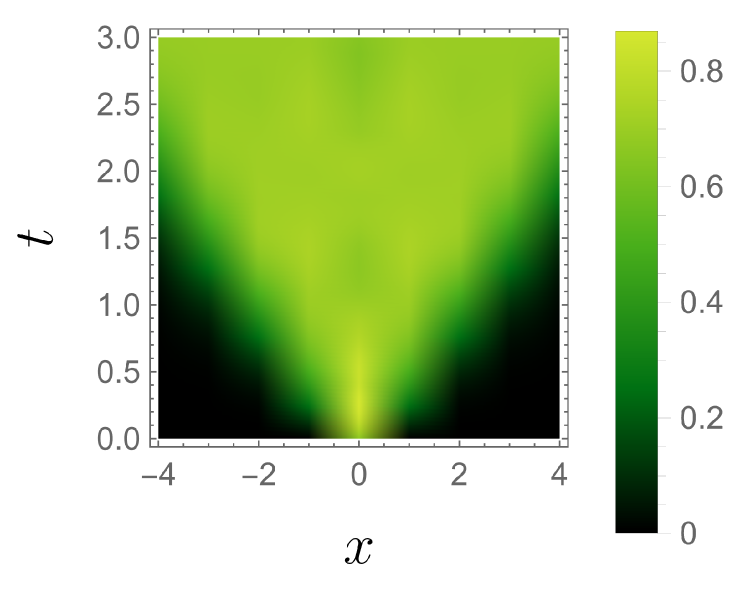
(b) $\gamma=0.3$

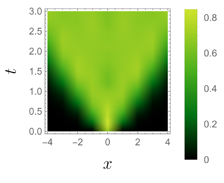
(c) $\gamma=0.6$

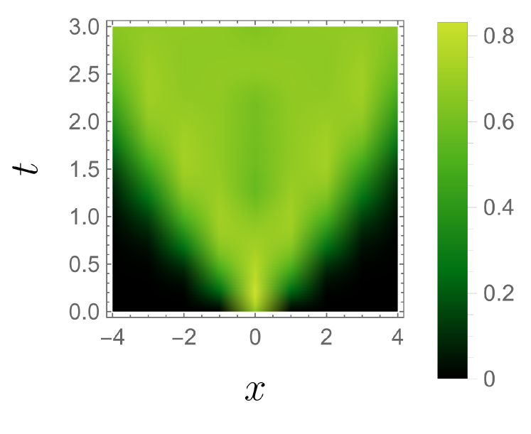
(d) $\gamma=0.9$

Figure 4: Plots of $\frac{1}{2}\|[\tilde{O}_{A}(t),O_{B}]\|/\|\tilde{O}_{A}(t)\|$ for $A=1$ and $B=x$, where $\tilde{O}_{A}(t)=U^{-1}O_{A}U$ is evolved under the imaginary TFIM. Results are averaged over $O_{A},O_{B}\in\{\sigma^{x},\sigma^{y},\sigma^{z}\}$. Plots demonstrate that this operator evolution preserves the LR bound. Decrease in LR velocity $v$ at large $\gamma$ corresponds to the transition in $H$ from chaotic to integrable dynamics that occurs at $\gamma\approx 1$.

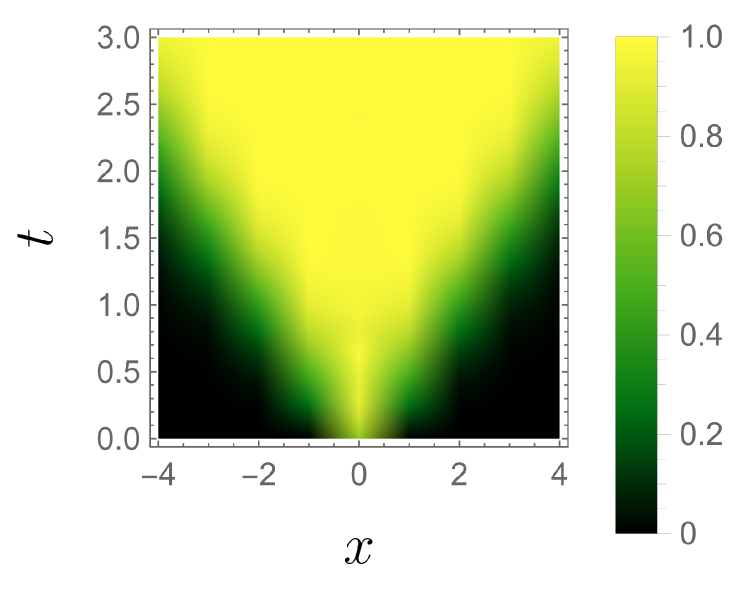
(a) $\gamma=0$

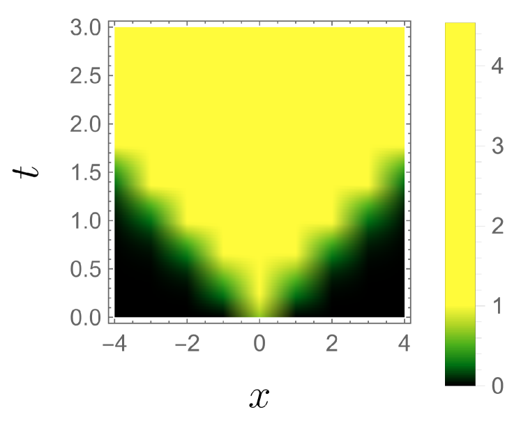
(b) $\gamma=0.3$

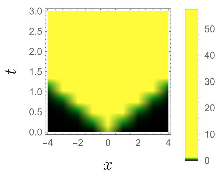
(c) $\gamma=0.6$

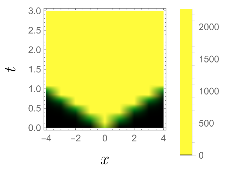
(d) $\gamma=0.9$

Figure 5: Plots of $\frac{1}{2}\|[\tilde{O}_{A}(t),O_{B}]\|$ for $A=1$ and $B=x$, where $\tilde{O}_{A}(t)=U^{-1}O_{A}U$ is evolved under the imaginary TFIM. Results are averaged over $O_{A},O_{B}\in\{\sigma^{x},\sigma^{y},\sigma^{z}\}$. Plots demonstrate that growth of $\|\tilde{O}_{A}(t)\|$ is dominated by exponential decay arising from the LR bound, and lightcone dynamics dominate, albeit at increased effective $v$.

Appendix E Entanglement Preparation Example

As an example case where the Metric CC LR bound is trivially satisfied, as discussed in Sec. VI.1, consider tripartite system $ABC$. Begin with an operator $O_{C}>0$ not proportional to the identity, and use Gram-Schmidt to extend the set $\{O_{C},\mathbb{I_{C}}\}$ to an orthonormal basis $\{\Gamma_{C}^{i}\}_{i=1}^{d^{2}}$ for $\mathscr{L(H}_{C})$. Notice that since $\mathbb{I}_{C}\in\text{span}\{\Gamma_{C}^{1},\Gamma_{C}^{2}\}$, $\text{Tr}[\Gamma_{C}^{k}]=\text{Tr}[\mathbb{I}_{C}\Gamma_{C}^{k}]=0$ for $k>2$. Then we can decompose arbitrary $\rho$ as

$$\rho=\sum_{k=1}^{d^{2}}a_{k}\rho_{AB}^{k}\otimes\Gamma_{C}^{k}$$ (E.1)

The $\rho_{AB}^{k}$ need not be density matrices in general, but for now assume they are. Taking $\eta_{C}=\Gamma_{C}^{1}$, basis orthonormality gives us

$$\begin{split}\text{Tr}_{C}[\rho]&=a_{1}\text{Tr}[\Gamma_{C}^{1}]\rho_{AB}^{1}+a_{2}\text{Tr}[\Gamma_{C}^{2}]\rho_{AB}^{2}\\ \text{Tr}_{C}[\rho\eta_{C}]&=a_{1}\rho_{AB}^{1}\end{split}$$ (E.2)

Any metric CC of the form $\langle O_{A},O_{B}\rangle_{\eta c}$ depends only on $\text{Tr}_{C}[\rho\eta]$. Thus if we take $\rho_{AB}^{1}$ product and $\eta=\eta_{A}\otimes\eta_{B}\otimes\eta_{C}$ for the given $\eta_{C}$, such a Metric CC will always be zero, trivially satisfying the Metric CC LR bound. Notice also this places no restriction on $\rho_{AB}^{2}$, which can be entangled to make $\rho_{AB}=\text{Tr}_{C}[\rho]$ entangled.

As an example of generation of long range entanglement, consider $\rho$ as in Eq. E.1 with $a_{1}=1$ and $a_{2}=0$, and product $\rho_{AB}^{1}$. In this case $\text{Tr}_{C}[\rho]$ is product. Pick some $H=H_{C}$ satisfying $H_{C}^{\dagger}\eta-\eta H_{C}=0$ for $\eta=\eta_{C}$. Finally, define $\delta\Gamma_{C}^{k}=H_{C}\Gamma_{C}^{k}-\Gamma_{C}^{k}H_{C}^{\dagger}$ and let $C_{jk}=\text{Tr}[\Gamma_{C}^{j{\dagger}}\delta\Gamma_{C}^{k}]$ be coefficients of $\delta\Gamma_{C}^{k}$ in the $\{\Gamma_{C}^{j}\}$ basis. Note that for all $k$, Hermiticity of $\Gamma_{C}^{1}\sim O_{C}>0$ gives

$$C_{1k}=C_{k1}=\text{Tr}[\Gamma_{C}^{k{\dagger}}\big{(}H_{C}\Gamma_{C}^{1}-\Gamma_{C}^{1}H_{C}^{\dagger}\big{)}]=0$$ (E.3)

Then, excluding normalization,

$$\begin{split}\text{Tr}_{C}[\partial_{t}\rho]&=-i\text{Tr}_{C}[H_{C}\rho-\rho H_{C}^{\dagger}]=-i\sum_{k\neq 2}a_{k}\rho_{AB}^{k}\text{Tr}[\delta\Gamma_{C}^{k}]\\ &=-i\sum_{k\neq 2}a_{k}\rho_{AB}^{k}\left(\sum_{j}C_{jk}\text{Tr}\left[\Gamma_{C}^{j}\right]\right)\\ &=-i\sum_{k>2}a_{k}\rho_{AB}^{k}\left(C_{2k}\text{Tr}\left[\Gamma_{C}^{2}\right]\right)\\ \end{split}$$ (E.4)

using $\text{Tr}[\Gamma_{C}^{j}]=0$ for $j>2$. Thus for entangled $\rho_{AB}^{k}$, $H_{C}$ generates entanglement between the $A,B$ subsystems at short times.

References

- Ashida et al. (2020) Y. Ashida, Z. Gong, and M. Ueda, Advances in Physics 69, 249 (2020).
- Matsumoto et al. (2020) N. Matsumoto, K. Kawabata, Y. Ashida, S. Furukawa, and M. Ueda, Physical Review Letters 125, 260601 (2020).
- Matsumoto et al. (2022) N. Matsumoto, M. Nakagawa, and M. Ueda, Phys. Rev. Res. 4, 033250 (2022).
- Gopalakrishnan and Gullans (2021) S. Gopalakrishnan and M. J. Gullans, Physical Review Letters 126, 170503 (2021).
- Ashida and Ueda (2018) Y. Ashida and M. Ueda, Physical Review Letters 120 (2018), 10.1103/physrevlett.120.185301.
- Lieb and Robinson (1972) E. H. Lieb and D. W. Robinson, Communications in Mathematical Physics 28, 251 (1972).
- Nachtergaele and Sims (2006a) B. Nachtergaele and R. Sims, Communications in Mathematical Physics 265, 119 (2006a).
- Bravyi et al. (2006) S. Bravyi, M. B. Hastings, and F. Verstraete, Physical Review Letters 97 (2006), 10.1103/PhysRevLett.97.050401.
- Poulin (2010) D. Poulin, Physical Review Letters 104, 190401 (2010).
- Hastings and Koma (2006) M. B. Hastings and T. Koma, Communications in Mathematical Physics 265, 781 (2006).
- Barch et al. (2023) B. Barch, N. Anand, J. Marshall, E. Rieffel, and P. Zanardi, Phys. Rev. B 108, 134305 (2023).
- Gharibyan et al. (2020) H. Gharibyan, M. Hanada, B. Swingle, and M. Tezuka, Physical Review E 102, 022213 (2020).
- Tran et al. (2017) M. C. Tran, J. R. Garrison, Z.-X. Gong, and A. V. Gorshkov, Physical Review A 96 (2017), 10.1103/physreva.96.052334.
- Wolf et al. (2008) M. M. Wolf, F. Verstraete, M. B. Hastings, and J. I. Cirac, Physical Review Letters 100 (2008), 10.1103/PhysRevLett.100.070502.
- Kudler-Flam et al. (2023) J. Kudler-Flam, L. Nie, and A. Vijay, “Rényi mutual information in quantum field theory, tensor networks, and gravity,” (2023), arXiv:2308.08600 [hep-th] .
- Scalet et al. (2021) S. O. Scalet, Á. M. Alhambra, G. Styliaris, and J. I. Cirac, Quantum 5, 541 (2021), arXiv:2103.01709 .
- Sergi and Zloshchastiev (2015) A. Sergi and K. G. Zloshchastiev, Physical Review A 91 (2015), 10.1103/physreva.91.062108.
- Mostafazadeh (2002) A. Mostafazadeh, Journal of Mathematical Physics 43, 205 (2002).
- Mostafazadeh (2003) A. Mostafazadeh, Czechoslovak Journal of Physics 53, 1079–1084 (2003).
- Ju et al. (2019) C.-Y. Ju, A. Miranowicz, G.-Y. Chen, and F. Nori, Physical Review A 100, 062118 (2019).
- Karuvade et al. (2022) S. Karuvade, A. Alase, and B. C. Sanders, Phys. Rev. Res. 4, 013016 (2022).
- Brun (2002) T. A. Brun, American Journal of Physics 70, 719 (2002).
- Bender and Boettcher (1998) C. M. Bender and S. Boettcher, Phys. Rev. Lett. 80, 5243 (1998).
- Bender et al. (2002) C. M. Bender, D. C. Brody, and H. F. Jones, Phys. Rev. Lett. 89, 270401 (2002).
- Fring and Moussa (2016) A. Fring and M. H. Y. Moussa, Phys. Rev. A 93, 042114 (2016).
- Dyson (1956) F. J. Dyson, Phys. Rev. 102, 1230 (1956).
- Biella and Schiró (2021) A. Biella and M. Schiró, Quantum 5, 528 (2021).
- Bañuls et al. (2011) M. C. Bañuls, J. I. Cirac, and M. B. Hastings, Phys. Rev. Lett. 106, 050405 (2011).
- Kim and Huse (2013) H. Kim and D. A. Huse, Phys. Rev. Lett. 111, 127205 (2013).
- Sylvester (1975) G. S. Sylvester, Communications in Mathematical Physics 42, 209 (1975).
- Zanardi (2001) P. Zanardi, Physical Review A 63 (2001), 10.1103/PhysRevA.63.040304.
- Lupo et al. (2008) C. Lupo, P. Aniello, and A. Scardicchio, Journal of Physics A: Mathematical and Theoretical 41, 415301 (2008).
- Aniello and Lupo (2009) P. Aniello and C. Lupo, Open Systems and Information Dynamics 16, 127–143 (2009).
- Popescu et al. (2006) S. Popescu, A. J. Short, and A. Winter, Nature Physics 2, 754 (2006).
- D'Alessio et al. (2016) L. D'Alessio, Y. Kafri, A. Polkovnikov, and M. Rigol, Advances in Physics 65, 239 (2016).
- Borgonovi et al. (2016) F. Borgonovi, F. Izrailev, L. Santos, and V. Zelevinsky, Physics Reports 626, 1 (2016).
- Dymarsky et al. (2018) A. Dymarsky, N. Lashkari, and H. Liu, Phys. Rev. E 97, 012140 (2018).
- Nachtergaele and Sims (2006b) B. Nachtergaele and R. Sims, Communications in Mathematical Physics 265, 119–130 (2006b).
- Nielsen and Chuang (2010) M. A. Nielsen and I. L. Chuang, Quantum Computation and Quantum Information, 10th ed. (Cambridge University Press, Cambridge ; New York, 2010).
- Li et al. (2018) Y. Li, X. Chen, and M. P. A. Fisher, Phys. Rev. B 98, 205136 (2018).
- Skinner et al. (2019) B. Skinner, J. Ruhman, and A. Nahum, Phys. Rev. X 9, 031009 (2019).
- Chan et al. (2019) A. Chan, R. M. Nandkishore, M. Pretko, and G. Smith, Phys. Rev. B 99, 224307 (2019).
- Li et al. (2019) Y. Li, X. Chen, and M. P. A. Fisher, Phys. Rev. B 100, 134306 (2019).
- Gullans and Huse (2020) M. J. Gullans and D. A. Huse, Phys. Rev. X 10, 041020 (2020).
- Choi et al. (2020) S. Choi, Y. Bao, X.-L. Qi, and E. Altman, Phys. Rev. Lett. 125, 030505 (2020).
- Ippoliti et al. (2021) M. Ippoliti, M. J. Gullans, S. Gopalakrishnan, D. A. Huse, and V. Khemani, Phys. Rev. X 11, 011030 (2021).
- Agarwal et al. (2023) K. D. Agarwal, T. K. Konar, L. G. C. Lakkaraju, and A. S. De, “Recognizing critical lines via entanglement in non-hermitian systems,” (2023), arXiv:2305.08374 [quant-ph] .
- Efetov (1997) K. B. Efetov, Physical Review Letters 79, 491 (1997).
- Chalker and Wang (1997) J. T. Chalker and Z. J. Wang, Physical Review Letters 79, 1797 (1997).
- Fyodorov et al. (1997) Y. V. Fyodorov, B. A. Khoruzhenko, and H.-J. Sommers, Physical Review Letters 79, 557 (1997).
- Fyodorov et al. (1998) Y. V. Fyodorov, H.-J. Sommers, and B. A. Khoruzhenko, Annales de l’I.H.P. Physique théorique 68, 449 (1998).
- Fyodorov and Sommers (2003) Y. V. Fyodorov and H.-J. Sommers, Journal of Physics A: Mathematical and General 36, 3303 (2003).
- Preskill (2012) J. Preskill, “Quantum computing and the entanglement frontier,” (2012).
- Anand and Zanardi (2022) N. Anand and P. Zanardi, Quantum 6, 746 (2022).