Approximation of arbitrarily high-order PDEs by first-order hyperbolic relaxation
Abstract
We present a framework for constructing a first-order hyperbolic system whose solution approximates that of a desired higher-order evolution equation. Constructions of this kind have received increasing interest in recent years, and are potentially useful as either analytical or computational tools for understanding the corresponding higher-order equation. We perform a systematic analysis of a family of linear model equations and show that for each member of this family there is a stable hyperbolic approximation whose solution converges to that of the model equation in a certain limit. We then show through several examples that this approach can be applied successfully to a very wide range of nonlinear PDEs of practical interest.
1 Introduction
Virtually any textbook on ordinary differential equations (ODEs) includes the observation that higher-order ODEs can be rewritten as systems of first-order ODEs. This can facilitate the analysis of ODE solutions by placing all ODEs in a unified framework, and it is particularly useful in the realm of numerical approximation, since it allows numerical analysts to focus exclusively on methods for first-order problems. High-order partial differential equations (PDEs) can also superficially be written in first-order form through the introduction of auxiliary variables. However, this is less useful since the theory and analysis of first-order PDEs is developed only for hyperbolic systems, but the first-order form of a higher-order PDE is in general not hyperbolic.
In this work we present a general technique for constructing a system of first-order hyperbolic PDEs (referred to as a hyperbolic relaxation, or hyperbolization) whose solution approximates that of a given system of higher-order evolution PDEs. We begin by presenting some motivating examples in Sections 1.2-1.3. We present these known examples in a way that suggests a more general approach but also raises some key questions. We then develop the general idea by studying a simple family of linear PDEs, in Section 2, where we answer the questions raised previously by determining the necessary and sufficient conditions for stability of the hyperbolization. This leads to a unique hyperbolization for each member of the family of high-order PDEs. In Section 3 we prove a convergence result relating the solution of the stable hyperbolic relaxation constructed in Section 2 and the original high-order PDE. In Section 4 we provide some examples suggesting that our approach can be successfully applied in a straightforward way to a wide range of nonlinear PDEs, including complex-valued equations, systems of equations, equations with mixed derivatives, and equations with up to (at least) 4th-order derivatives. We conclude in Section 5 with a discussion of important open questions.
1.1 Prior work and motivation
The idea of approximation by a hyperbolic system dates back at least to the works of Cattaneo and Vernotte [5, 25], who constructed a hyperbolic relaxation of the heat equation. Much more recently, Toro & Montecinos [24] gave a general approach to and analysis of hyperbolization of second-order advection-reaction-diffusion equations, including a detailed study of the efficiency of the numerical solution of the hyperbolized model compared to the original model. Mazaheri et. al. [21] provided a general approach to hyperbolization of scalar PDEs that include first-, second-, and third-order spatial derivatives (i.e., advection-diffusion-dispersion equations), and demonstrated it through application to the KdV and Burgers equations. Many other hyperbolized versions of PDE models have been proposed, e.g. for Korteweg-de Vries (KdV) [3], Benjamin-Bona-Mahoney (BBM) [15], Serre-Green-Naghdi (SGN) [13, 12, 2], multilayer dispersive shallow water equations [7], the compressible Navier-Stokes equations [20], the Euler-Korteweg equation (in hydrodynamic form) [10], and a range of additional dispersive wave equations [1, 16, 11, 9, 6, 14], as well as elliptic equations [22].
Most of the foregoing works explore hyperbolization as a means to remove numerical stiffness. For an evolution PDE with spatial derivatives of order , stability of any explicit numerical method requires a time step , and typically for it is best to use implicit numerical solvers. For PDEs with mixed space and time derivatives, a numerical solution is usually obtained by performing an elliptic solve at each step. In all of these cases, the complexity and per-step cost of numerical solvers is substantially increased compared to that of first-order hyperbolic systems, which can typically be solved efficiently using only explicit methods. Replacing the stiff high-order PDE by a first order PDE is therefore quite appealing. However, the hyperbolic approximations referenced above all have the property that they approximate the higher-order system accurately only when certain characteristic speeds become large. The stiffness of the original problem can thus return through the mechanism of these large characteristic speeds, so it is not clear a priori that solution of a hyperbolic approximation is more efficient. Many existing works on hyperbolization do not consider this question. The most thorough theoretical comparison of efficiency in this regard shows that (for certain second-order equations) a hyperbolized approximation can be solved more efficiently than the original problem when the spatial grid is relatively coarse, but it becomes inefficient on finer grids [24]. We consider the relative computational efficiency of hyperbolization plus discretization versus direct high-order PDE discretization to be an important matter for future work.
Another potential advantage of hyperbolic formulations is more straightforward: imposition of boundary conditions – especially non-reflecting boundary conditions, which are more developed for hyperbolic problems than for general PDEs. For instance, in [3], some dispersive wave equations are approximated by hyperbolic systems in order to formulate absorbing boundary conditions using perfectly matched layers. As we will see, hyperbolized PDEs do require additional initial conditions, but these can usually be obtained in a very natural way and are similar to those required for PDEs with multiple temporal derivatives.
Finally, a fundamental motivation for approximation by hyperbolic equations is that of causality. PDEs with higher-order terms allow for action at a distance or arbitrarily fast propagation of high-wavenumber perturbations, and are thus incompatible with the theory of relativity. In contrast, for hyperbolic PDEs perturbations travel at or below some maximum speed. This served as the motivation for some of the early work on hyperbolic relaxation of the heat equation.
The approach introduced by Jin and Xin [18] is also referred to as hyperbolic relaxation, but it differs fundamentally from the concept dicsussed herein. In Jin-Xin relaxation, the relaxation terms are usually algebraic, the starting point is a first-order nonlinear hyperbolic system, and the result is a dissipative approximation. Here we start from higher-order (not hyperbolic) PDEs, we use relaxation terms that involve differential operators, and the resulting approximation is non-dissipative if the original problem is non-dissipative. See Section 1.2.1 for discussion of one connection between these ideas.
Before entering into further details, we present two introductory examples that have appeared before and serve to motivate the technique developed later in the present work.
1.2 The Heat Equation
The oldest example of hyperbolization of which we are aware was proposed independently by Cattaneo [5] and Vernotte [25]. The heat equation
| (1) |
can be written superficially as a first-order system by introducing the auxiliary variable :
| (2a) | ||||
| (2b) | ||||
The hyperbolic formulation is obtained by relaxing the constraint (2b) as part of an evolution equation for :
| (3a) | ||||
| (3b) | ||||
The first equation comes directly from (1), while the second equation causes to relax toward . The parameter controls the scale of this relaxation time; as , one expects that the solution of (3) will tend to that of (1). Defining , system (3) can be written in the form
| (4) |
where is diagonalizable with eigenvalues , so this system is hyperbolic. If we assume a solution of the form , we find that the full dispersion relation for (3) is
| (5) |
resulting in
| (6) | ||||
| (7) |
We see that , so that the dispersion relation of (1) is approximately preserved. The accuracy of the approximation is seen to improve as . Notice that has negative real part proportional to , so there is a spurious mode but it decays quickly if is small. Note also that if , then has a real part and a negative imaginary part. This means that solutions are stable but we should expect to see wave-like behavior for high wavenumbers or when is large. Note that if we take , there exist exponentially growing solutions.
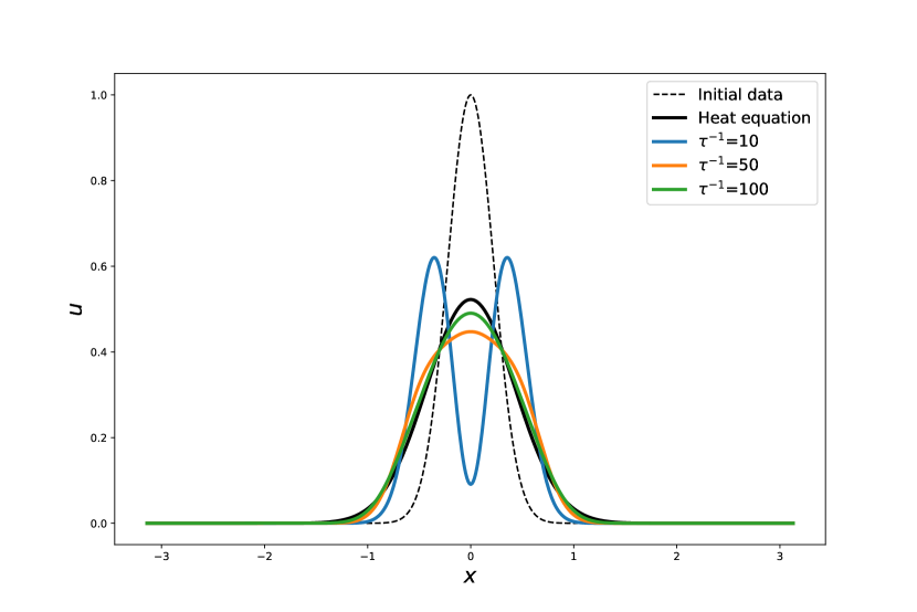
Figure 1 shows a comparison of the solution of the heat equation with that of its hyperbolic approximation, with a Gaussian initial condition. For large values of , the solution behaves similarly to that of the wave equation, with the initial pulse breaking into two waves propagating in opposite directions, consistent with the dispersion relation analysis above. For smaller values of , the solution behaves very similarly to that of the heat equation. We remark that wave-like heat transport under certain conditions has long been theorized and recently been experimentally observed [8, 26].
1.2.1 Relation to Jin-Xin Relaxation
Jin & Xin [18] introduced a technique for approximating a hyperbolic PDE
by the hyperbolic system
| (8a) | ||||
| (8b) | ||||
We can formally cast the hyperbolic relaxation of the heat equation in this form by writing and taking . The result is equivalent to the system (3) (though is defined with the opposite sign). In [18] it was shown that the solution of (8) is approximated by that of
and as a result the stability of (8) requires the sub-characteristic condition . Taking the same approach for the heat equation and including the term in the evolution equation for , one finds that the solution of the resulting relaxation system is approximated (to first order in ) by
| (9) |
This equation is stable for any non-negative (and in fact for any ), so in particular one can simply take as we have done above.
For hyperbolic relaxation of higher-order PDEs (such as that in the next section), there is not a straightforward relationship to Jin-Xin relaxation.
1.3 The Korteweg-de Vries Equation
Next, consider the Korteweg-de Vries (KdV) equation:
| (10) |
We introduce and , so that . We use to write a first-order approximation of (10), and introduce evolution equations for that incorporate relaxation terms that tend to enforce the foregoing approximations
| (11a) | ||||
| (11b) | ||||
| (11c) | ||||
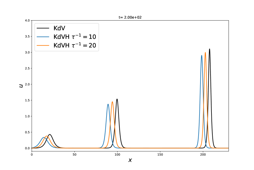
As before, we require and we expect that the solution of (11) approaches that of (10) as . The system (11) was introduced previously as a means to implement non-reflecting numerical boundary conditions [3, Eqn. (13)]. A comparison of the solutions of the KdV equation (10) and its hyperbolic approximation (11) for two different values of is shown in Figure 2.
Although the formulation of (11) seems fairly natural based on our discussion and the similar handling of the heat equation above, it is worth noting that it involves certain choices that at this point might seem arbitrary. Why are the right-hand sides of (11b) and (11c) chosen as they are, rather than the reverse? Why are the signs of those terms chosen as they are? How would the properties of the system change if these signs or order were modified? In the next section, we will answer these questions and devise a general approach to formulating similar hyperbolizations.
The main contributions of the present work are:
-
•
construction of stable hyperbolic approximations to a family of arbitrarily high-order PDEs;
-
•
proof of pointwise convergence of the hyperbolic relaxation in Fourier space;
-
•
successful application of the technique to multiple problems outside the scope of what has been done before.
2 A general approach to hyperbolization
In this section we provide an approach to hyperbolization that generalizes the examples above and other examples in the literature. Let us consider the Cauchy problem for the linear model equation
| (12a) | ||||
| (12b) | ||||
| (12c) | ||||
The restriction on the sign ensures that all solutions remain bounded for . We introduce new variables for . Then we can approximate (12) by the system of equations
| (13a) | |||||
| (13b) | |||||
Here we take , , and the sequence is a permutation of the integers from 1 to . The idea is to introduce an evolution equation for each , and incorporate in each equation one of the constraints . We now investigate how one should choose which constraint appears in which evolution equation (i.e., we determine the permutation sequence ) and the signs of the constraint multipliers.
For instance, consider the linearized KdV equation:
| (14) |
We have , and the system (13) takes one of the two following forms:
| (15a) | ||||
| (15b) | ||||
| (15c) | ||||
or
| (16a) | ||||
| (16b) | ||||
| (16c) | ||||
Altogether the above equations represent 8 possible choices. The question immediately arises: which of these systems (if any) is preferable? At a glance, the most natural choice is (15) with ”-” on the right side of the second and third equation, since then these equations directly impose that and relax to and . However, that system is in fact unstable. As we will see, only one of these 8 systems is stable, and in fact for each value of , there is a unique choice of permutation and signs in (13) such that the resulting approximation of (12) is stable.
2.1 Necessary Conditions for Stability
We can write (13) in matrix form as
| (17a) | |||||||
| where | |||||||
| (17b) | |||||||
and is a signed permutation matrix111A (real) signed permutation matrix is square with all entries equal to -1, 0 or +1, and has exactly one non-zero entry in each row and each column. of size . Applying the ansatz , we find that the dispersion relation is given by the solution of
| (18) |
Since the time-dependence of the ansatz has the form , the solution is stable only if the imaginary part of is non-positive. It is convenient to consider two necessary conditions for stability: stability for , and stability for large . It turns out that it is sufficient to consider the special case , in which case we can write (18) as
| (19) |
2.1.1 Low-wavenumber stability
For , the dispersion relation (19) reduces to
| (20) |
so stability is obtained only if all eigenvalues of lie in the closed left half-plane. The matrix has one eigenvalue equal to zero and the rest equal to the eigenvalues of , so we must choose such that its eigenvalues are in the closed left half-plane. The following lemma characterizes such permutation matrices.
Lemma 1.
Let be a real signed permutation matrix with all eigenvalues in the closed left half-plane. Then
| (21) |
where is skew-symmetric (), and is a diagonal matrix with all entries equal to 1 or 0.
Proof.
Any permutation can be decomposed in terms of disjoint cycles, and the set of eigenvalues of the permutation is just the union of the eigenvalues of each cycle. The eigenvalues of a cycle of length are just the th roots of unity. The same can be said for signed permutation matrices, except that the eigenvalues of a signed cycle of length are in general th roots of either or . The only sets of roots of that lie fully in the closed left half-plane are itself and the square roots of . Therefore, must be the product of cycles of length 1 and/or 2 only, and the 2-cycle components must be antisymmetric. ∎
2.1.2 High-wavenumber stability
As , the dispersion relation tends to the solution of
| (22) |
i.e. the dispersion relation of the homogeneous hyperbolic system , whose solutions are stable if and only if has only real eigenvalues.
Lemma 2.
Let be a real signed permutation matrix and let be given by (17b) with . If has only real eigenvalues then
| (23) |
where is symmetric and is a diagonal matrix with all entries equal to or 0.
Proof.
The proof is similar to that of Lemma 1. Notice that itself is a signed permutation matrix, so to have only real eigenvalues it must consist only of 2-cycles with equal signs and/or 1-cycles. ∎
It is possible to prove an even stronger result: must be anti-diagonal (with non-zero entries only for ). But Lemma 2 is sufficient to prove the main result in the next section.
2.2 The unique stable hyperbolization
Let us continue our example above with the linearized KdV equation (14). Now is a matrix and from Lemma 1 we see that either
| (24) |
From the stability condition (23) for large , we see that the only possibility is
| (25) |
yielding the hyperbolized system (corresponding to (16) with minus in the second equation and plus in the third)
Returning to the general equation (12), since , condition (23) implies . Then condition (21) implies ; hence (23) implies , and so forth. Continuing in this manner, it can be shown that the only way to satisfy the necessary stability conditions is to choose (and ) to be anti-diagonal, with entries
| (26) |
Having applied these necessary conditions, we can now ask if the system (17) with (26) is indeed stable for intermediate values of and for all values of .
Proof.
The “only if” part has been proven already by consideration of the necessary conditions above. It remains to prove sufficiency.
From the general dispersion relation (18) we see that is given by the eigenvalues of , where . Since is symmetric and is skew-symmetric, is Hermitian. Furthermore, since we can write
from which we see that is similar to a Hermitian matrix, hence it has only real eigenvalues. Since is real, the hyperbolized system is stable for all . ∎
The unique stable hyperbolic system, combining (17) with (26), is
| (27a) | |||||
| (27b) | |||||
| (27c) | |||||
Note that (27) is stable for satisfying (12c). It is not stable for even with , since the model equation (12a) is unstable in that case.
In order to approximate the solution of an initial value problem for equation (12), one must also supply initial data for . The natural choice is
| (28) |
2.3 General Linear Scalar Evolution PDEs
Next we consider the more general model equation
| (29) |
where we assume the values are such that solutions remain bounded; in particular this implies that and if is even then . There are many ways to modify (27) to account for the lower-order derivative terms present in (29), since each term could be replaced by either or . Taking always the first choice yields
| (30a) | |||||
| (30b) | |||||
while taking always the second choice yields
| (31a) | |||||
| (31b) | |||||
In the following analysis, and in the examples in Section 4, we follow (31). It is an open question whether there is some advantage to using (30), or some combination of the two.
Theorem 2.
Proof.
Consider the hyperbolization of (29) given by (33). This system can be written in the form (17) but with and replaced by
| (32) |
For , stability requires that the eigenvalues of lie in the left half-plane. The eigenvalues of are the same as those of , but with the zero eigenvalue replaced by . Hence it is necessary that the eigenvalues of lie in the closed left half-plane and that ; the latter condition is required for stability of the original PDE (29).
For large , stability requires that the eigenvalues of be real. Using Laplace expansions, it can be shown that if is given by (26) then the characteristic polynomial of takes the form
The roots of this polynomial are all real. ∎
Taking as in (26) with the hyperbolization (31) yields the system
| (33a) | |||||
| (33b) | |||||
| (33c) | |||||
While we have not found a way to generalize Theorem 1 and prove stability of (33) for all wavenumbers, Theorem 2 suggests that it is a promising choice. Computational experiments indicate that this choice may in fact be stable for all wavenumbers whenever the original problem (29) is stable.
2.4 Further generalizations
In Section 4 we will apply the approach above to more general PDEs, including nonlinear equations and equations with mixed space-time derivatives. For nonlinear problems, it is natural to require stability of the linearized dispersion relation, which leads again to the choice of signed permutation matrix determined above. For problems with mixed space- and time-derivatives, we will again use linear stability as our guiding principle. A detailed investigation of the hyperbolization of such PDEs, and of systems of PDEs, is left to future work.
3 Accuracy of the hyperbolic approximation
As illustrated and discussed above, the solution of the hyperbolized PDE is expected to converge to that of the original PDE as . What is the size of the hyperbolization error , and how quickly does it vanish as decreases?
For the hyperbolized heat equation (3), using equality of mixed partial derivatives we find that
| (34) |
Using equality of mixed partial derivatives again, one obtains , so that (see (9))
| (35) |
This suggests that the hyperbolized solution converges linearly to that of the original equation, and also that one should take
in order to ensure that the error terms are small compared to the leading order terms. For the initial data shown in Figure 1, this suggests one should take , which is in general agreement with the results shown. As time advances, the ratio of derivatives becomes smaller, and one correspondingly observes improved agreement between the solutions (even those with large values of ) after long enough time.
For the family of linear PDEs (12), we have the following result.
Theorem 3.
Theorem 3 shows that the Fourier transform of the hyperbolized solution converges to that of the original problem pointwise. To prove convergence of the solution itself would require more detailed estimates of the difference between the two as a function of the wavenumber . Such an extension, as well as extension to more general PDEs, is left to future work.
3.1 Proof of Theorem 3
The initial data (28) can be written
| (38) |
Let be defined as in (17) with defined by (26). Let ; i.e.
| (39) |
Lemma 3.
The matrix has the following properties:
-
1.
has an eigenvalue zero of multiplicity one, with corresponding eigenvector , where .
-
2.
is diagonalizable with distinct eigenvalues, and the remaining eigenvectors are orthogonal to .
-
3.
is diagonalizable, and all of its eigenvalues have zero real part, for all .
-
4.
has an eigenvector , with eigenvalue .
-
5.
Let denote the matrix of right eigenvectors of . Then
Proof.
Properties 1-2: Taking , the first row of vanishes, so has a zero eigenvalue. The corresponding eigenvector can be found by direct computation. Let denote the matrix obtained by removing the first row and last column of . The remaining eigenvalues of are those of , which has determinant 1, and thus has no zero eigenvalues. Furthermore, is skew-Hermitian, so it is diagonalizable with purely imaginary eigenvalues. To see that the eigenvalues of are distinct, let denote any of its eigenvalues. Then the submatrix obtained by removing the first row and last column of is non-singular, so this eigenvalue has multiplicity one.
Property 3: This follows from the fact that is similar to a skew-Hermitian matrix (see the proof of Theorem 1.
Property 4: The first statement follows from continuous dependence of the eigenvector on . The left eigenvector corresponding to the zero eigenvalue of is . Then [23, Thm. IV.2.3] states that the corresponding eigenvalue of is
Property 5: This follows from the fact that is diagonalizable with distinct eigenvalues; see [19, Thm. 8, p. 130]. ∎
Finally, we prove Theorem 3.
Proof.
The solution of (12) can be written as where is given by the solution of the initial-value ODEs
Here is given by (39). By Lemma 3 property 3, we can write , ordering the eigenvalues to that the top-left entry of is the value referred to in Lemma 3, property 4. Then the solution of (40) is
Note that the entries of remain bounded even for and arbitrary , due to Lemma 3 property 3. So using Lemma 3 property 4, we can write
where and denotes a diagonal matrix whose entries are bounded as and whose top left entry vanishes, so .
4 Examples
In this section we apply and extend the foregoing theory in relation to some widely-studied nonlinear PDEs. Whereas the examples from the introduction follow our theory in a straightforward way, here we focus on examples that have additional complications.
In the following examples, we use a Fourier pseudospectral collocation method in space and explicit 3rd-order Runge-Kutta integration in time. The code to reproduce each example is available online222http://github.com/ketch/hyperbolization-RR.
4.1 The Nonlinear Schrodinger Equation
Let us consider the nonlinear Schrodinger (NLS) equation
| (41) |
with linear dispersion relation . We introduce and . In order to obtain a stable hyperbolic system, in this case we use an imaginary multiplier (), yielding the system
| (42a) | ||||
| (42b) | ||||
Writing this system in the form (4) shows that the characteristic speeds are . Linearizing about yields the dispersion relation
so that
Expanding the square root about shows that one of the roots is equal to , which approximates the dispersion relation of the linear Schrodinger equation.
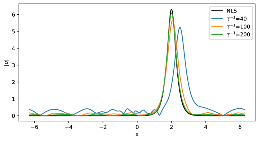
Figure 3 shows a comparison between the solution of the NLS equation (41) and those of the hyperbolic NLS equation (42), with varying values of . The initial condition is a soliton solution of (41):
The solution shown is computed at .
4.2 The Camassa-Holm Equation
Next we consider the Camassa-Holm (CH) equation
| (43) |
with initial data [4], and the periodic boundary condition . Figure 7 in [4] illustrates that the solution of this problem. The initial parabolic pulse steepens and then breaks into a train of peakon solitons, which move at speeds proportional to their amplitudes. This example of hyperbolization is interesting in that it contains two different third-order derivative terms, one of which is nonlinear. Introducing equations for and in the same way as for the KdV equation, we write
This system is not in the usual hyperbolic form, since the first equation contains time derivatives of both and . This is easily remedied by adding times the last equation to the first, leading to the hyperbolized CH (CHH) system
| (44a) | ||||
| (44b) | ||||
| (44c) | ||||
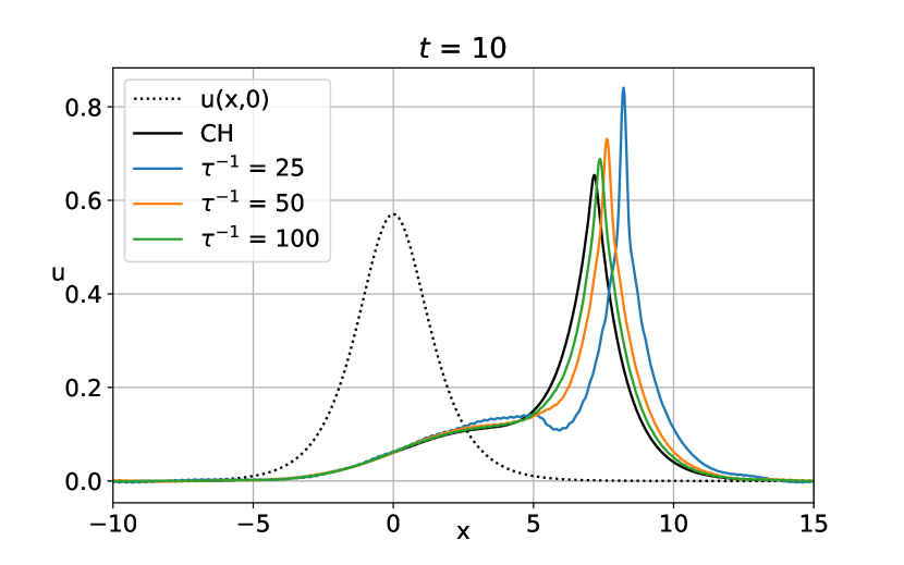
Interestingly, the linear dispersion relation for this system is stable for both positive and negative values of . We choose and solve the corresponding hyperbolized systems on the domain using a pseudo-spectral semi-discretization in space with spatial grid points and the SSPRK33 method in time, with . The solution of the original CH equation is also computed using the pseudo-spectral semi-discretization in space and the SSPRK33 method in time, employing the same number of grid points in space. Figure 4 illustrates that the solution of the CHH tends to the solution of the original CH equation as the hyperbolization parameter decreases.
4.3 The Kuramoto-Sivashinsky Equation
In this section we hyperbolize the Kuramoto-Sivashinsky (KS) equation
| (45) |
To our knowledge, this is the first example of hyperbolization of an equation with derivatives of order greater than three. The linear dispersion relation for (45) is
Note that for small wavenumbers , the linearized KS equation is unstable; only the presence of the nonlinear term prevents blowup of solutions. It is natural to ask whether this feature prevents the generation of a stable hyperbolization.
Based on the analysis in Section 2.1, we propose the hyperbolic system
| (46a) | ||||
| (46b) | ||||
| (46c) | ||||
| (46d) | ||||
with . Solutions of (45) are known to exhibit both periodic behavior and chaotic behavior, depending on the problem setup. A preliminary study of solutions of (46) shows that it behaves similarly, yielding periodic or chaotic solutions under similar circumstances. The solutions of (46) are observed to converge to those of (45) as , when the solution is not chaotic. Under conditions in which (45) becomes chaotic, that of (46) seems to do the same, and the time to onset of chaos is nearly the same.
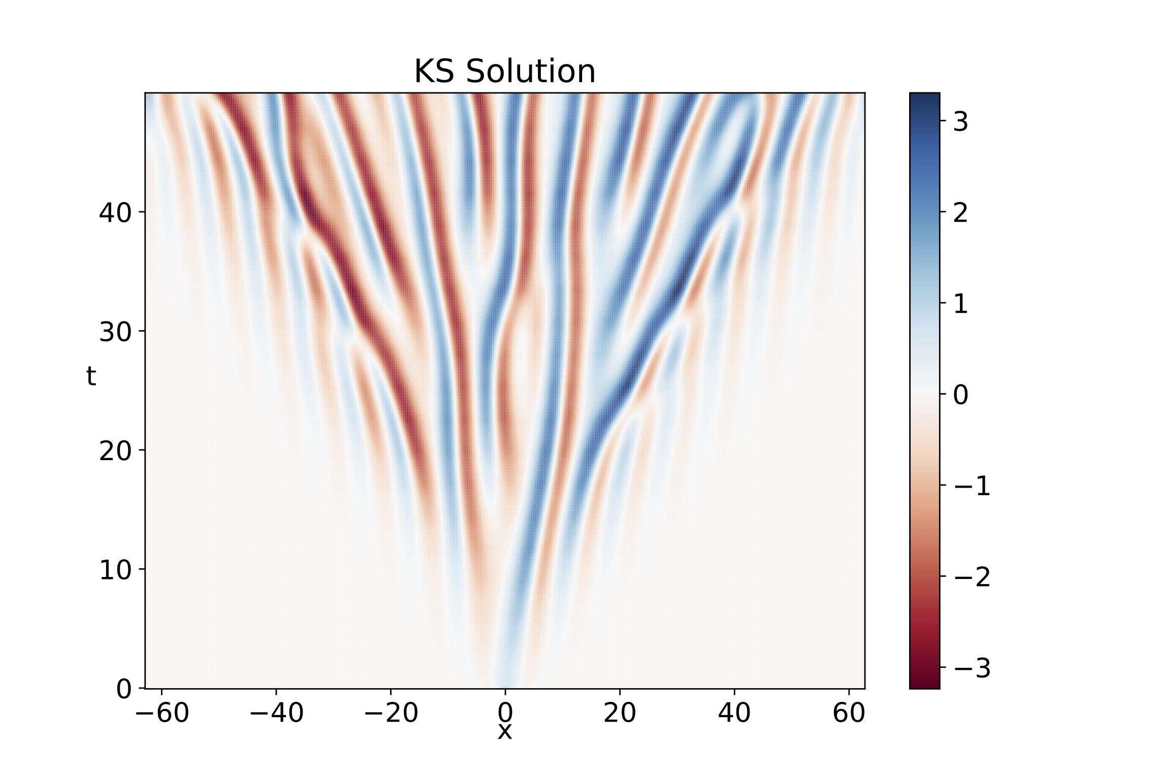
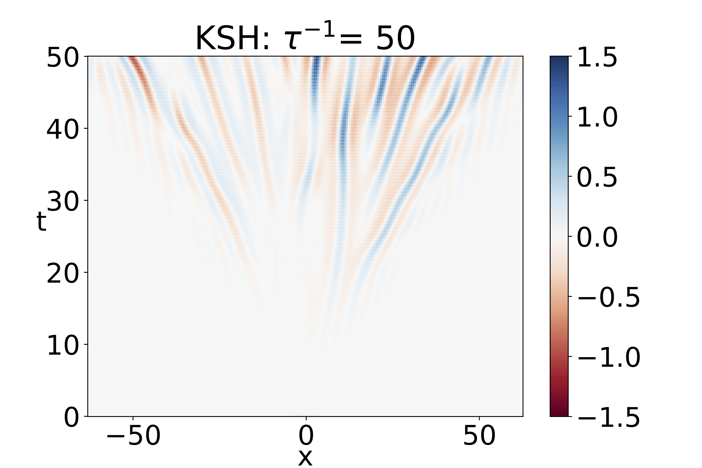
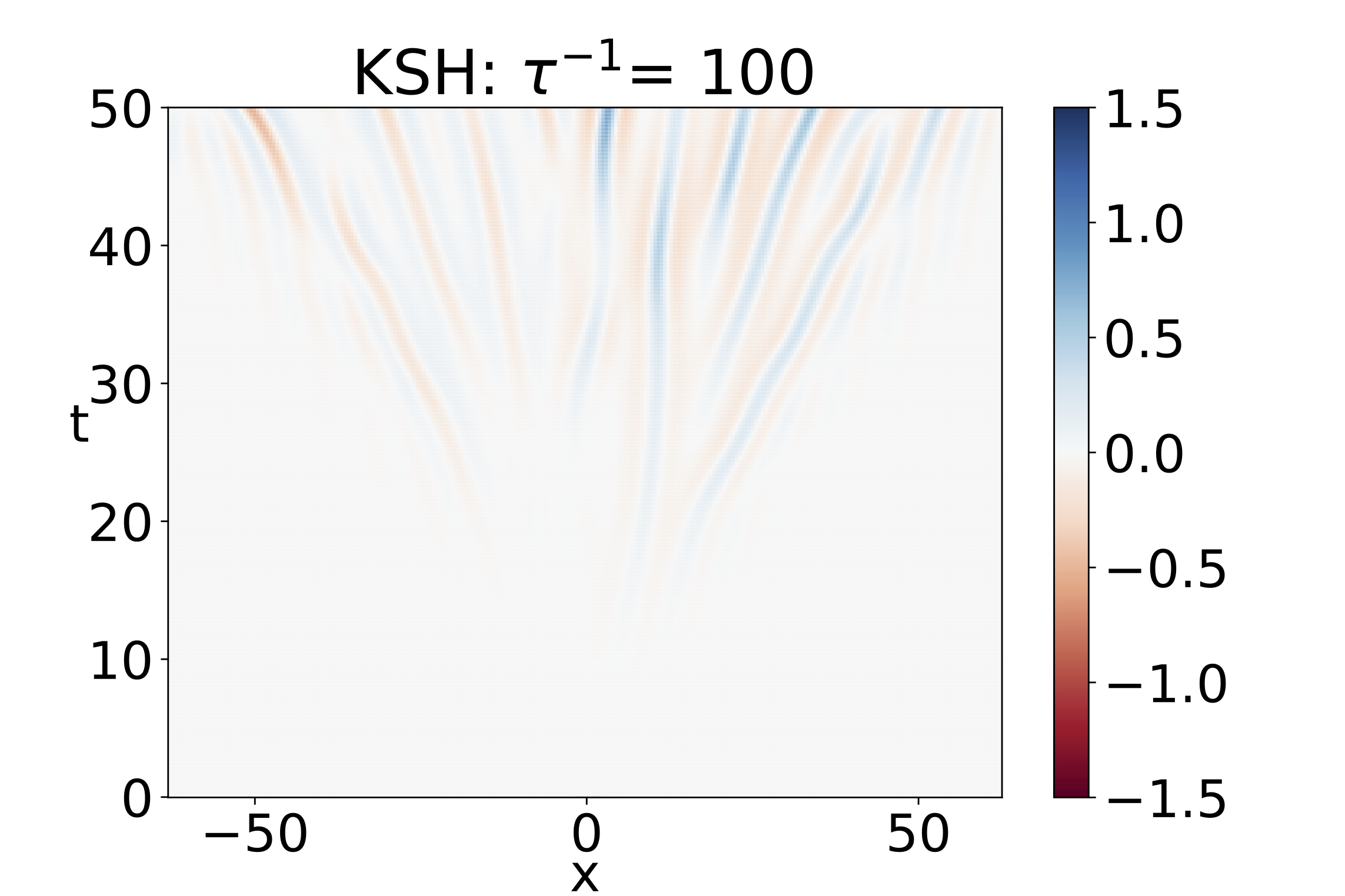
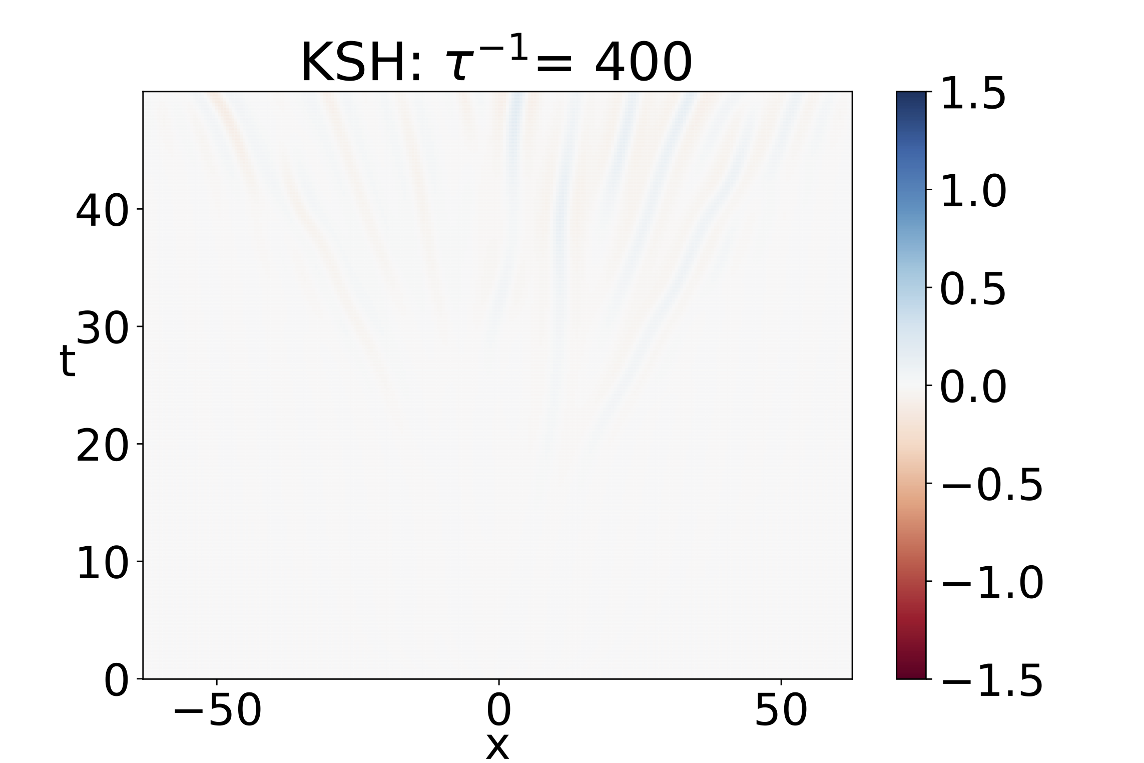
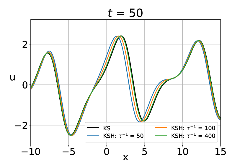
Here we present an example demonstrating the convergence of the solution of the hyperbolized Kuramoto-Sivashinsky (KSH) equation to the solution of the original Kuramoto-Sivashinsky (KS) equation as tends to 0. We consider the problem on the domain with the Gaussian initial condition and periodic boundary conditions. Figure 5 shows the solution to the KS equation (45) with a Gaussian initial condition, up to time . Each KSH system with different relaxation parameters is solved using the pseudospectral method with grid points in space and the classical 4th-order RK method in time, up to a final time of . The corresponding solution of the original KS equation at each time is also obtained using the pseudospectral method in space and a 4th-order ImEx method in time, with the same resolution in space and time. Figure 6 shows the point-wise errors of the solution of the KSH equation compared to the KS equation (45), and we observe that the solution of the KSH equation converges to the solution of the KS equation as tends to 0. The convergence of the solution of the KSH to the solution of the KS equation at is shown in the bottom right panel.
5 Discussion
While the first work on hyperbolization of high-order PDEs dates back to the 1950s, work in this area has accelerated in the last 15 years, during which a variety of techniques in this vein have been applied to a number of different models. Some of these recent works can be seen as particular cases of the general technique discussed herein. Awareness and understanding of hyperbolization as a general tool is likely to facilitate its application to an increasing number of models.
Herein we have shown for the first time that a stable hyperbolization exists for PDEs of arbitrarily high order. We have focused on scalar evolution equations, in order to narrow the scope enough to facilitate development of a comprehensive theory. But a wide variety of other PDE models – including elliptic problems, evolution problems with hyperbolic constraints, and general systems of high-order PDEs – are susceptible to a similar treatment.
Even for scalar evolution equations, there are many interesting open questions and avenues for further research in this area, including:
-
•
General design and analysis of energy conservation or other structural properties in hyperbolized systems;
-
•
development of efficient numerical discretizations;
-
•
more detailed understanding of the relative efficiency of hyperbolized approximations.
Furthermore, the construction of the hyperbolized equations admits additional freedom that has been explored in the literature only in the context of specific models; for instance the inclusion of additional convective terms in the auxiliary equations, or the use of multiple different relaxation times .
It is also worth considering the possibility of gaining insight into higher-order PDE models and solutions by analyzing their hyperbolized counterparts. An interesting corollary of our results is that higher-order PDE models that violate local causality can be approximated arbitrarily well by models that respect causality.
Since hyperbolic PDEs admit similarity solutions (Riemann solutions) that can often be solved by semi-analytical means, the study of the Riemann problem for hyperbolized systems might yield novel insights. For one existing study of this kind, see [17].
References
- [1] M Antuono, V Liapidevskii, and M Brocchini. Dispersive nonlinear shallow-water equations. Studies in Applied Mathematics, 122(1):1–28, 2009.
- [2] Caterina Bassi, Luca Bonaventura, Saray Busto, and Michael Dumbser. A hyperbolic reformulation of the Serre-Green-Naghdi model for general bottom topographies. Computers & Fluids, 212:104716, 2020.
- [3] Christophe Besse, Sergey Gavrilyuk, Maria Kazakova, and Pascal Noble. Perfectly matched layers methods for mixed hyperbolic–dispersive equations. Water Waves, 4(3):313–343, 2022.
- [4] R. Camassa, D. D. Holm, and J. M. Hyman. A new integrable shallow water equation. Advances in Applied Mechanics, 31:1–33, 1994.
- [5] Carlo Cattaneo. Sur une forme de l’equation de la chaleur eliminant la paradoxe d’une propagation instantantee. Compt. Rendu, 247:431–433, 1958.
- [6] AA Chesnokov, VE Ermishina, and V Yu Liapidevskii. Strongly non-linear Boussinesq-type model of the dynamics of internal solitary waves propagating in a multilayer stratified fluid. Physics of Fluids, 35(7), 2023.
- [7] Alexander Chesnokov and Trieu Hai Nguyen. Hyperbolic model for free surface shallow water flows with effects of dispersion, vorticity and topography. Computers & Fluids, 189:13–23, 2019.
- [8] Marvin Chester. Second sound in solids. Physical Review, 131(5):2013, 1963.
- [9] Firas Dhaouadi and Michael Dumbser. A first order hyperbolic reformulation of the Navier-Stokes-Korteweg system based on the GPR model and an augmented Lagrangian approach. Journal of Computational Physics, 470:111544, 2022.
- [10] Firas Dhaouadi, Nicolas Favrie, and Sergey Gavrilyuk. Extended Lagrangian approach for the defocusing nonlinear Schrödinger equation. Studies in Applied Mathematics, 142(3):336–358, 2019.
- [11] Firas Dhaouadi, Sergey Gavrilyuk, and Jean-Paul Vila. Hyperbolic relaxation models for thin films down an inclined plane. Applied Mathematics and Computation, 433:127378, 2022.
- [12] Cipriano Escalante, Michael Dumbser, and Manuel J Castro. An efficient hyperbolic relaxation system for dispersive non-hydrostatic water waves and its solution with high order discontinuous Galerkin schemes. Journal of Computational Physics, 394:385–416, 2019.
- [13] N Favrie and S Gavrilyuk. A rapid numerical method for solving Serre–Green–Naghdi equations describing long free surface gravity waves. Nonlinearity, 30(7):2718, 2017.
- [14] Sergey Gavrilyuk, Boniface Nkonga, and Keh-Ming Shyue. The conduit equation: hyperbolic approximation and generalized Riemann problem. Available at SSRN 4724161, 2024.
- [15] Sergey Gavrilyuk and Keh-Ming Shyue. Hyperbolic approximation of the BBM equation. Nonlinearity, 35(3):1447, 2022.
- [16] Giovanna Grosso, Matteo Antuono, and Maurizio Brocchini. Dispersive nonlinear shallow-water equations: some preliminary numerical results. Journal of Engineering Mathematics, 67:71–84, 2010.
- [17] Giovanna Grosso, Matteo Antuono, and Eleuterio Toro. The Riemann problem for the dispersive nonlinear shallow water equations. Communications in Computational Physics, 7(1):64, 2010.
- [18] Shi Jin and Zhouping Xin. The relaxation schemes for systems of conservation laws in arbitrary space dimensions. Communications on pure and applied mathematics, 48(3):235–276, 1995.
- [19] Peter D Lax. Linear algebra and its applications, volume 78. John Wiley & Sons, 2007.
- [20] Lingquan Li, Jialin Lou, Hong Luo, and Hiroaki Nishikawa. A new formulation of hyperbolic Navier-Stokes solver based on finite volume method on arbitrary grids. In 2018 Fluid Dynamics Conference, page 4160, 2018.
- [21] Alireza Mazaheri, Mario Ricchiuto, and Hiroaki Nishikawa. A first-order hyperbolic system approach for dispersion. J. Comput. Phys., 321(Supplement C):593–605, 2016.
- [22] Hannes R Rüter, David Hilditch, Marcus Bugner, and Bernd Brügmann. Hyperbolic relaxation method for elliptic equations. Physical Review D, 98(8):084044, 2018.
- [23] G. W. Stewart and Ji-Guang Sun. Matrix Perturbation Theory. Academic Press, 1990.
- [24] Eleuterio F Toro and Gino I Montecinos. Advection-diffusion-reaction equations: hyperbolization and high-order ADER discretizations. SIAM Journal on Scientific Computing, 36(5):A2423–A2457, 2014.
- [25] Pierre Vernotte. Les paradoxes de la theorie continue de l’equation de la chaleur. Comptes rendus, 246:3154, 1958.
- [26] Zhenjie Yan, Parth B Patel, Biswaroop Mukherjee, Chris J Vale, Richard J Fletcher, and Martin W Zwierlein. Thermography of the superfluid transition in a strongly interacting Fermi gas. Science, 383(6683):629–633, 2024.