When does compositional structure yield compositional generalization? A kernel theory.

Abstract

Compositional generalization (the ability to respond correctly to novel combinations of familiar components) is thought to be a cornerstone of intelligent behavior. Compositionally structured (e.g. disentangled) representations are essential for this; however, the conditions under which they yield compositional generalization remain unclear. To address this gap, we present a general theory of compositional generalization in kernel models with fixed, potentially nonlinear representations (which also applies to neural networks in the “lazy regime”). We prove that these models are functionally limited to adding up values assigned to conjunctions/combinations of components that have been seen during training (“conjunction-wise additivity”), and identify novel compositionality failure modes that arise from the data and model structure, even for disentangled inputs. For models in the representation learning (or “rich”) regime, we show that networks can generalize on an important non-additive task (associative inference), and give a mechanistic explanation for why. Finally, we validate our theory empirically, showing that it captures the behavior of deep neural networks trained on a set of compositional tasks. In sum, our theory characterizes the principles giving rise to compositional generalization in kernel models and shows how representation learning can overcome their limitations. We further provide a formally grounded, novel generalization class for compositional tasks that highlights fundamental differences in the required learning mechanisms (conjunction-wise additivity).

1 Introduction

Humans’ understanding of the world is inherently compositional: once familiar with the concepts “pink” and “elephant,” we can immediately imagine a pink elephant. Stitching together concepts in this way allows humans to generalize far beyond our prior experience, preparing us to cope with unfamiliar situations and imagine things that do not yet exist [1, 2]. Understanding the basis of compositional generalization in humans and animals, and building it into machine learning models, is a long-standing and historically vexing problem [3, 4, 5, 6, 7]. Accordingly, a broad range of studies have investigated the conditions under which compositionally structured (i.e. “disentangled”) representations can be learned [8, 9, 10, 11, 12, 13, 14]. However, it remains unclear whether learning these representations is actually useful: while some work suggests that disentangled representations improve compositional generalization [12, 15, 16, 17], other studies challenge this view [11, 18, 19, 20]. In particular, it is often unclear how insights on a certain compositional task generalize to others, as the relationship among them remains unclear [6].

To clarify when compositionally structured representations yield compositional generalization, we define a family of compositional tasks, theoretically analyse the compositional generalization of kernel models, and then validate our theory in several relevant deep neural network architectures. Kernel models are an important class of statistical models in their own right (describing e.g. linear readout fine-tuning), provide a simplified approximation to neural network learning under certain conditions [21, 22], and more broadly have provided fundamental insight into generalization behavior in humans and machine learning models [23, 24, 25, 26].

Despite the broad importance and relative simplicity of kernel models, it remains largely unclear how they generalize on compositional tasks [[, though see ]; see Section 2]abbe_generalization_2023,lippl_mathematical_2024. To address this gap, we present a theory of compositional generalization in kernel models. We define a new generalization class for compositional tasks and show that characterizing kernel models on such tasks helps us understand realistic neural network architectures. Our specific contributions are as follows:

• We prove fundamental limits on the generalization behavior of kernel models with disentangled inputs, showing that they are constrained to summing up values implicitly assigned to each component or combination of components seen during training. We define the class of compositional tasks with this form as “conjunction-wise additive” (Section 4.1).

• We define a metric to quantify how salient different component “conjunctions” (entangled features unique to component combinations) are in the representation (Section 4.2).

• For conjunction-wise additive tasks, we then highlight two important failure modes impacting generalization (memorization leak and shortcut bias) (Section 4.3), which describe how biases in the training data can limit compositional generalization even for kernel models with disentangled inputs.

• We validate our theory in several deep neural network architectures, showing that it captures their behavior on conjunction-wise additive tasks (Section 4.4).

• Finally, we show how feature learning can overcome certain limitations of kernel models and learn non-additive tasks (Section 4.5).

2 Related work

Compositional generalization. Compositionality is an important theme across human and machine reasoning problems, including visual reasoning [29, 30, 31, 32, 33], language production [6], rule learning [34, 35], image generation [36], and robotics [37]. Recent breakthroughs (especially in language and computer vision) have led to massive improvements in models’ compositional capacities, but in some cases, these models still fail spectacularly [38, 39, 40, 41, 42]. Attempts to improve compositional generalization often leverage meta-learning [43, 44, 45, 46, 47], or modular architectures, in the hopes that different modules will specialize for different components [48]. End-to-end training of these architectures often does not result in the desired modular specialization [49, 50, 51]; notably, [52] theoretically clarify the necessary conditions for correct modular specialization and compositional generalization in hypernetworks.

Here we highlight that kernel models add up values assigned to each combination of features (or “conjunction”) seen during training. Notably, constraining a network to be additive can be sufficient for compositional generalization [53, 54]. Even without such constraints, language models encode many semantic concepts in an additive manner [55, 56]. Conjunctive codes (representations specific to a particular feature combination), on the other hand, have a long history in neuroscience [57, 58], and are theoretically linked to forming highly specific, episodic memories.

Kernel and rich regime. Prior work has revealed two key strategies by which deep neural networks learn [22, 59]. In the kernel (or “lazy”) regime (which can be induced with large initial weights or wide networks), the networks’ learning is well approximated by gradient descent on a model with a fixed representation [21]. In the rich regime (brought forth, for example, by small initial weights, small width, low-rank connectivity, or loss functions like cross-entropy), the networks learn structured (i.e. abstract and sparse) representations over the course of learning [60, 59, 61, 62, 63, 64, 65]. This is often suggested to give rise to better generalization and more human-like behavior in neural networks [66, 67, 68].

When using gradient descent, ridge regression, or similar learning algorithms to train the readout weights of a model $f_{w}(x)=w^{T}r(x)$, this model depends on its representation $r(x)$ only through its induced kernel $K(x,x^{\prime})=\langle r(x),r(x^{\prime})\rangle$ [69]. Specifically, when trained on a dataset $\{(x_{i},y_{i})\}_{i=1}^{n}$, it can be written in its “dual form” as

$$\textstyle f_{a}(x)=\sum_{i=1}^{n}a_{i}K(x,x_{i}).$$ (1)

Gradient descent and ridge regression learn the readout weights that describe the training data with minimal $\ell_{2}$-norm; this is also true of neural networks in the kernel regime [70, 71, 72]. Norm minimization is a standard theoretical framework for analyzing how representational geometry influences generalization [25, 73] and we here apply it to the compositional task setting. This is similar to [28] who characterize model behavior on a specific compositional task (transitive ordering) and [27] who characterize the inductive bias of norm minimization for inputs with binary components in the limit of infinite components. Compared to [27, 28], we analyze a broader range of compositional tasks and derive exact constraints for finite numbers of components.

Memorization and shortcut learning. The relationship between memorization and generalization has been extensively studied [74, 75]. Memorization sometimes refers to models’ tendency to learn difficult (and even randomly labeled) examples [76, 77, 78]. This may improve generalization on long-tailed data [79, 80]. Alternately, memorization can refer to models learning a narrow mapping on the training data rather than a generalizable rule [81, 82]. We here find models tend to partially memorize their training data even when they extract the correct rule at the same time. Relatedly, [51] [51] analyze how the learning dynamics in deep linear networks can give rise to this phenomenon.

Shortcut learning refers to models exploiting spurious correlations between certain features and the target to learn the training data and has been essential for understanding why the performance of deep neural networks can drop substantially when tested out-of-distribution [83]. Models are more likely to use shortcut features that are easily extracted from the input and highly predictive of the output [84, 85, 86]. Shortcut learning has also been connected to the implicit bias of gradient descent [87, 88]. Our findings highlight a particular compositional shortcut: models tend to use a more salient, partially predictive component conjunction (memorizing the remaining data) over the fully predictive but less salient ground-truth conjunction.

3 Model and task setup

3.1 Task space

We assume that our model extracts a set of components $z=\sum_{c=1}^{C}z_{c}$ from its input $x$. Each $z_{c}\in Z_{c}\subset\mathbb{R}^{d}$ is drawn from a discrete set of possible components. For example, $z$ could specify the color and shape of an object, and the background color of an image (Fig. 1a). Alternately, $z$ may express different words in an input sentence (“the red sphere is in front of the blue background”). We assume that each component $z_{c}$ is represented in an orthogonal subspace (e.g. by concatenating representations of individual components, Fig. 1a). Further, because we consider categorical components, we can assume that for each component $c$, all representations $z_{c}\in Z_{c}$ have equal magnitude $m_{c}$ and are represented with equal similarity $\rho_{c}$ to alternative component values. The target, $y\in\mathbb{R}$, is some function of $z$ (see Section 3.3). After training models on certain component combinations $Z^{\text{train}}\subset Z=\prod_{c=1}^{C}Z_{c}$, we assess generalization on all other combinations, $Z^{\text{test}}:=Z\setminus Z^{\text{train}}$ to understand how biases in the training data affect compositional generalization.

3.2 Models

Linear readout models. We first consider kernel models which take in a disentangled representation $z$, apply a nonlinear transform $\phi(z)\in\mathbb{R}^{h}$ and learn a linear readout using gradient descent or ridge regression, $f_{w}(x):=w^{T}\phi(z)$ (Fig. 1a). For $\phi$, we consider a neural network with random weights:

Definition 3.1.

Given an input $z\in\mathbb{R}^{d}$, a network depth $L\geq 2$, and a set of widths $H_{1},\dotsc,H_{L}\in\mathbb{N}$, we define a neural network by recursively defining the operation $\phi^{(l)}$ of the $l^{\text{th}}$ layer as

$$a^{(0)}:=z,\quad a^{(l)}:=\phi^{(l)}(a^{(l-1)}):=\sigma\left(\tfrac{1}{\sqrt{H_{l}}}\left(W^{(l)}a^{(l-1)}+b^{(l)}\right)\right),\quad W^{(l)}\in\mathbb{R}^{H_{l}\times H_{l-1}}$$ (2)

where $W^{(l)}$ and $b^{(l)}$ are i.i.d. sampled from a random distribution and $\sigma:\mathbb{R}\to\mathbb{R}$ is a nonlinearity. The complete transform is then given by $\phi:=\phi^{(L)}\circ\dotsb\circ\phi^{(1)}$.

We consider the infinite-width limit of $\phi$, where $H_{1},\dotsc,H_{L-1}\to\infty$ (the order of these limits does not matter). Note that our model setup includes as a special case the random feature model studied by [27] [27] and further captures training through backpropagation in the kernel/lazy regime.

Deep neural network models. Additionally, we consider different deep neural network architectures used for vision (convolutional networks, ResNets, and Vision Transformers, Section 4.4) and ReLU networks trained through backpropagation (Section 4.5).

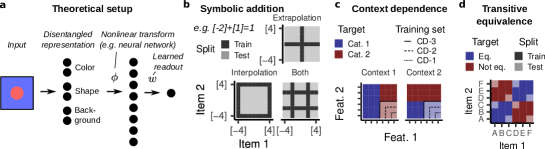
Figure 1: a, Theoretical setup: we consider a disentangled representation of the input, followed by a nonlinear transform $\phi$ and a learned linear readout $w$. b, Training sets for symbolic addition. The grid represents nine components with associated values $-4,-3,\dotsc,4$. Each tile represents a data point in the training set. c, Context dependence. In context 1, feat. 1 determines the category; in context 2, feat. 2 determines the category. The training sets leave out different subsets of the lower right orthant. d, Transitive equivalence: six items are split up into two arbitrary equivalence classes (e.g. A,B,C and D,E,F) and generalization requires transitive inference over equivalence classes.

3.3 Example tasks

In addition to deriving a general theory, we consider a set of example tasks that are important building blocks for compositional reasoning in machine learning and cognitive science (Appendix D discusses additional tasks including logical operations and partial exposure):

Symbolic addition. Many tasks involve inferring a magnitude associated with different underlying components (e.g. handwritten digits) [89, 90]. We consider two components $(z_{1},z_{2})$ with unobserved assigned values $v_{1}(I_{1})$ and $v_{2}(I_{2})$. The target is the sum of those values: $y=v_{1}(z_{1})+v_{2}(z_{2})$. After sufficient exposition to individual items, a model with an additive structure can generalize to novel combinations of items [54]. In particular, we consider nine input elements $[-4],[-3],\dotsc,[4]$ with associated values $-4,-3,\dotsc,4$ and training sets containing all pairs where at least one component is equal to a certain subset of values. This can require interpolation, extrapolation, or both (Fig. 1b).

Context dependence. The relevance of different stimuli often depends on the context we are in. Taking into account this context is a crucial aspect of cognition in humans and animals [91, 92, 93, 34]. We therefore consider a task with three input components $(z_{\text{co}},z_{f1},z_{f2})$. The context ($z_{\text{co}}$) has two possible values specifying whether $z_{f1}$ or $z_{f2}$ determine the response. Both features have six possible values which are split up in two categories. If the model has learned this context dependence, it should be able to generalize to novel feature combinations. We evaluate on the orthant for which $z_{f1}$ indicates Cat. 2 and $z_{f2}$ indicates Cat. 1. In the most extreme generalization test (CD-3), we leave out the entire orthant, in easier versions we leave out conjunctions of two or one of those features (CD-2 and CD-1) (Fig. 1c).

Transitive equivalence. Relational reasoning is an important instance of compositional generalization and often involves extending the learned relations to new item combinations [94, 4]. Given an unobserved (and arbitrary) equivalence relation, the task is to determine whether two presented items $(z_{1},z_{2})$ are equivalent. The model should generalize to novel item pairs using transitivity ($A=B$ and $B=C$ imply $A=C$) (Fig. 1d). This is an important instance of relational cognition (often studied as “associative inference” in cognitive science [95, 96]). Note that prior work has found that kernel models often successfully generalize a transitive ordering relation [28].

4 Results

4.1 Kernel models with compositional structure are conjunction-wise additive

Our primary theoretical contribution in this work is to characterize the full range of compositional computations that can be implemented by kernel models with disentangled inputs: specifically, they assign a value to each combination of components seen during training and generalize to test inputs by adding up the relevant combinations’ values. We call this motif “conjunction-wise additivity.” Below we formally state our finding and then explain its implications.

We first note that the kernel of the disentangled representation, $K(z,z^{\prime})=z^{T}z^{\prime}$, only depends on the components for which the two inputs are overlapping, $O(z,z^{\prime}):=\left\{c|z_{c}=z_{c}^{\prime}\right\}$ where $c\in\{1,\dotsc,C\}$. This is necessitated by the fact that separate components are represented in orthogonal subspaces. We call any representation satisfying this criterion “compositionally structured.” Notably, the hidden representation $\phi(z)$ is also compositionally structured (in the infinite-width limit). This is because the kernel of the neural network’s representation, $K_{\phi}(z,z^{\prime}):=\phi(z)^{T}\phi(z)$, only depends on the inputs $z,z^{\prime}$ through their kernel $K(z,z^{\prime})$ and thus conserves this property [[]; see Appendix B]cho_kernel_2009,tsuchida_invariance_2018,tsuchida_richer_2019,han_fast_2022.

Intriguingly, we find that any kernel model with a compositionally structured representation is constrained to be conjunction-wise additive. To state this finding, we define, for each $z\in Z$, the set of conjunctions for which $z$ overlaps with some element in the training set $z^{\text{tr}}\in Z^{\text{train}}$,

$$O(z|Z^{\text{train}}):=\left\{S\subseteq\{1,\dotsc,C\}|\exists z^{\text{tr}}\in Z^{\text{train}}\text{ s.t. }S\subseteq O(z,z^{\text{tr}})\right\}.$$ (3)

We then prove:

Theorem 4.1.

For $z\in Z$, any kernel model $f$ with a compositionally structured representation and training data $Z^{\text{train}}$ can be expressed as a sum of functions $f_{S}$ over all conjunctions $S\in O(z|Z^{\text{train}})$, where each $f_{S}$ associates a value with each unique combination of features $z_{c}$ for $c\in S$:

$$\textstyle f(z)=\sum_{S\in\mathcal{O}(z|Z^{\text{train}})}f_{S}(z_{S}),\quad z_{S}:=(z_{c})_{c\in S}.$$ (4)

We prove the theorem in Appendix A. Intuitively, it holds because the model associates a distinct weight vector with each conjunction/combination of components. The weight vectors associated with conjunctions not seen during training remain at their initial value and can therefore not be used.

To understand the theorem’s implications, we first consider a direct linear readout, $f(z)=w^{T}z$. This constrains the model to adding up a value for each component (“component-wise additivity”):

$$\textstyle f(z)=w^{T}z=w^{T}\sum_{c=1}^{C}z_{c}=\sum_{c=1}^{C}f_{c}(z_{c}),\quad f_{c}(z_{c}):=w^{T}z_{c}.$$ (5)

Component-wise additivity is a strict subset of conjunction-wise additivity (each $f_{S}$ depending on more than one component is set to zero). It lets the model generalize perfectly on component-wise additive tasks like symbolic addition. However, it also prevents the model from learning any training set that is not component-wise additive, including context dependence and transitive equivalence.

The nonlinear transform $\phi$ can overcome this constraint [101, 102, 103, 104]. Indeed, conjunction-wise additive functions more broadly can learn arbitrary training data, as the full conjunction $S=\{1,\dotsc,C\}$ is in $O(z|Z^{\text{train}})$ for each $z\in Z^{\text{train}}$ and $f_{S}(z)$ can take on a distinct value for each $z$. However, for $z\in Z^{\text{test}}$ the full conjunction is not in $O(z|Z^{\text{train}})$. Thus, while conjunction-wise additivity (unlike component-wise additivity) does not impose a constraint on the kinds of training data the model can learn, it does impose constraints on the kinds of generalizations it can implement.

In particular, for inputs with two components, $f(z)=f_{1}(z_{1})+f_{2}(z_{2})+f_{12}(z)$ for $z\in Z^{\text{train}}$. However, for $z\in Z^{\text{test}}$, $f_{12}(z)$ falls away and kernel models are constrained to an additive computation: $f(z)=f_{1}(z_{1})+f_{2}(z_{2})$. Thus, they cannot generalize on any non-additive task, including transitive equivalence: while they learn the training data (using $f_{12}(z)$), they cannot generalize to the test data.

For inputs with more than two components, a conjunction-wise additive computation does not just encode each component and their full conjunction, but also partial conjunctions between components (e.g. 12, 13, and 23 for three components). For test inputs, the model can still not rely on the full conjunction (123), but it can rely on any partial conjunction it may have seen before.

To see whether such a model can, in principle, generalize on a given task, we must 1) identify the overlaps with the training set, $\mathcal{O}(z|Z^{\text{train}})$, and 2) determine whether the target can be written as a conjunction-wise sum. For example, for context dependence, for all new test inputs, we have seen the context-feature conjunctions (i.e. 12 and 13), but not the feature-feature conjunction (i.e. 23). As a result, model behavior on the test set can be written as $f(z)=f_{1}(z_{\text{co}})+f_{2}(z_{f1})+f_{3}(z_{f2})+f_{12}(z_{\text{co}},z_{f1})+f_{13}(z_{\text{co}},z_{f2})$. While the task is not component-wise additive, we can use $f_{12}$ and $f_{13}$ to encode the task: $f_{12}(z_{\text{co}},z_{f1})$ encodes the target when the context $z_{\text{co}}$ indicates the first feature $z_{f1}$ as relevant and is zero otherwise; $f_{13}(z_{\text{co}},z_{f2})$ works in the opposite way.

Hence, conjunction-wise additivity not only tells us whether kernel models with compositionally structured representations can solve a certain task, but also how they solve it. Further, it tells us to make a task non-additive: in Section D.2.3, we describe a modification that makes context dependence non-additive by requiring generalizations to novel context-feature conjunctions.

Importantly, conjunction-wise additivity only determines whether certain compositional generalizations are, in principle, feasible. Model generalization also depends on whether the model identifies the correct conjunction-wise function. We discuss this in the next two sections.

4.2 Overlap salience characterizes compositional representational geometry

Model generalization is determined by how prominently different component conjunctions are represented. This is measured by the similarity $K(S)$ between inputs with overlap $S\subseteq\{1,\dotsc,C\}$. $K(S)$ depends on responses to that particular conjunction $S$ as well as all of its sub-conjunctions $S^{\prime}\subsetneq S$. We thus define the scalar salience of an overlap $S$ as its unique contribution. We then normalize this salience, so all saliences add up to one:

Definition 4.2.

For a representation with kernel $K$ and a conjunction $S\subseteq\{1,\dotsc,C\}$, we define

$$\textstyle\overline{\text{Sal}}(\emptyset):=K(\emptyset),\quad\overline{\text{Sal}}(S):=K(S)-\sum_{S^{\prime}\subsetneq S}\overline{\text{Sal}}(S^{\prime}),\quad{\text{Sal}}(S)=\tfrac{\overline{\text{Sal}}(S)}{\sum_{\emptyset\neq S\subseteq\{1,\dotsc,C\}}\overline{\text{Sal}}(S)}.$$ (6)

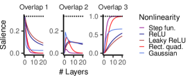
Figure 2: Normalized salience (i.e. $\text{Sal}_{C}(k)$) for neural networks with random weights and different nonlinearities for inputs with three components.

We now analyze how the representational salience evolves over different layers of a random network, considering an uncorrelated disentangled correlation with equal magnitudes (i.e. $\rho_{c}=0$ and $m_{c}=m_{c^{\prime}}$) (see Section B.2 for analysis beyond these assumptions). In that case, the salience only depends on the overlap size $k:=|S|$ and we denote it by $\text{Sal}_{C}(k)$.

Notably, conjunctions are only encoded and can only be used if they have non-zero salience. In particular, the disentangled representation has zero salience for all conjunctions of more than one component. As the network gets deeper, the salience of these conjunctions increases. In fact, for (leaky) ReLU networks, the salience of the full conjunction converges to one:

Proposition 4.3.

For a random neural network with a (leaky) ReLU nonlinearity, as $L\to\infty$, $\text{Sal}_{C}(k)\to 0$ for $k<C$ and $\text{Sal}_{C}(C)\to 1$.

We prove this statement in Section B.1. Empirically, we find that $\text{Sal}_{C}(C)$ indeed increases with depth, whereas $\text{Sal}_{C}(1)$ decreases (Fig. 2). The salience of intermediate conjunctions (e.g. $\text{Sal}_{3}(2)$) first increases and then decreases, its trajectory depending on the nonlinearity.

4.3 Kernel models suffer from two failure modes: memorization leak and shortcut bias

In Section 4.1, we found that kernel models sum up values assigned to different component conjunctions. This leaves ambiguous, however, whether they generalize correctly, as they can learn the training data using different combinations of conjunctions. Notably, kernel models trained with gradient descent or ridge regression generally learn the readout weights with minimal $\ell_{2}$-norm [[, Section 2;]]soudry_implicit_2018,gunasekar_characterizing_2018,ji_gradient_2020. This inductive bias gives rise to weights that are distributed across different predictive features. For in-distribution generalization, this is often useful, as it allows us to integrate different kinds of evidence. However, for compositional generalization, we often need to rely on a small group of conjunctions and the tendency towards distributed weights causes generalization failures.

Here we highlight two particular failure modes arising from this. First, the full conjunctions always serve as predictive features (“memorization leak”). Second, the model can often use statistical shortcuts to predict parts of the training set, using the full conjunction to learn the rest (“shortcut bias”). Below we explain how these failure modes impact symbolic addition and context dependence.

Symbolic addition suffers from a memorization leak. The functional form $f(z)=f_{1}(z_{1})+f_{2}(z_{2})+f_{12}(z)$ implies that using the full conjunction $f_{12}(z)$ to learn the training set will necessarily distort the inferred values $f_{1}(z_{1}),f_{2}(z_{2})$. This, in turn, negatively impacts generalization on the test set. To analyze the impact of such a memorization leak in detail, we characterize model behavior on symbolic addition analytically for training sets that are balanced around zero:

Proposition 4.4.

Consider input elements in $\{[v]\}_{v\in\mathcal{V}},\mathcal{V}\subset\mathbb{R}$ with associated values $v$. We assume that the training set contains all pairs such that at least one component is $z_{c}\in\{[w]\}_{w\in\mathcal{W}},\mathcal{W}\subset\mathbb{R}$ and that the average value in both $\mathcal{V}$ and $\mathcal{W}$ is zero. Then, model behavior on the test set is given by

$$f([i],[j])=m(i+j),\quad m:=\tfrac{p\cdot\text{Sal}_{2}(1)}{1+(p-2)\text{Sal}_{2}(1)},\quad p:=|\mathcal{W}|$$ (7)

We prove the proposition in Section D.1.1. It implies that for any representation that encodes the conjunction (i.e. has $\text{Sal}_{2}(2)>0$ and therefore $\text{Sal}_{2}(1)<\tfrac{1}{2}$), the model underestimates the inferred values by a constant factor $m<1$. Further, $m$ decreases for smaller $\text{Sal}_{2}(1)$ and increases for larger training set size (Fig. 3a,b). Perhaps surprisingly, these are the only two factors influencing $m$. In particular, while we often assume that interpolation is easier than extrapolation, these changes in training set do not impact model behavior here. We found qualitatively similar behavior for randomly generated, dispersed training sets (Section D.1.2, Fig. 7).

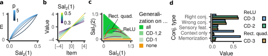
Figure 3: Kernel models’ behavior on (a,b) symbolic addition and (c,d) context dependence. a, Factor $m$ distorting the inferred values as a function of $\text{Sal}_{2}(1)$ and the training set size $p=|\mathcal{W}|$. b, Inferred values on extrapolation task. c, Variants of context dependence for which different representational saliences yield successful generalization. Trajectories of networks with different nonlinearities are highlighted (color scale see Fig. 2). d, Inferred coefficients of the different conjunction types for two example representations: a network with three layers and a rectified linear or quadratic nonlinearity.

Notably, because the full conjunction can always be used to learn the training set, the memorization leak impacts a broad range of compositional tasks, including partial exposure (Section D.4).

Context dependence suffers from a shortcut bias. Next, we empirically analyzed model generalization on context dependence across different representational geometries and training sets. We found that on a given task, each model either generalizes with 100% or 0% accuracy. For CD-3, the model only generalizes when $\text{Sal}_{3}(2)$ is high relative to $\text{Sal}_{3}(1)$ (Fig. 3c). As a result, whether the network generalizes is highly sensitive to the nonlinearity and depth of the network. In contrast, for CD-2 and CD-1, a much wider range of representational geometries generalizes successfully.

To better understand this, we analyzed the total magnitude of model weights associated with the different conjunctions. Notably, there are many possible conjunctions the model could rely on (see Section D.2.4). In particular, context $1$ is more likely to have the target $y=1$ and context $2$ is more likely to have target $y=-1$. The model may thus rely on this statistical shortcut, using the full conjunction to memorize the remaining training data. Indeed, we found that representations that generalized unsuccessfully on CD-3 consistently had a high weight associated with the context component and the full conjunction (Fig. 3d). Notably, for CD-3, the context shortcut yields an accuracy of $\tfrac{2}{3}$. This explains why when $\text{Sal}_{3}(1)$ and $\text{Sal}_{3}(3)$ are high relative to $\text{Sal}_{3}(2)$, the model uses the context-driven shortcut together with the full conjunction, resulting in a failure to generalize. For CD-2, the context-driven shortcut only results in an accuracy of $\tfrac{9}{16}$, making it much less useful. This explains why only very low $\text{Sal}_{3}(2)$ yields failure to generalize on CD-2 or CD-1.

Our analysis illustrates how conjunction-wise additivity lets us identify component conjunctions that yield a shortcut. The representational salience of these conjunctions and the extent to which they can explain the training set then helps us understand when this shortcut impacts generalization.

4.4 Conjunction-wise additivity can describe generalization behavior in deep neural networks

So far, we have analyzed kernel models, for their analytical tractability. We conjecture that large-scale neural network architectures with more complex, interrelated inputs might also be prone to implementing a conjunction-wise additive computation. In that case, our analyis of the kernel models would shed light on when the statistics of the training data enable or prevent compositional generalization in deep neural networks as well. To test our conjecture, we trained convolutional networks (ConvNets, [105]) on a version of the tasks with concatenated MNIST digits [106] and residual networks (ResNets, [107]) and Vision Transformers (ViTs, [108]) on a version of the tasks with concatenated CIFAR-10 images [109]. We considered the same tasks except that each component was now given by images of a particular category, rather than being a single instance. Notably, different image categories are not necessarily equally correlated with each other. To control for this, we randomly permuted the assignment of categories to components for each ($n=10$) experiment. To compare the network behaviors to our theoretical predictions, we fit a conjunction-wise additive function to the network output using linear regression (“additivity analysis”; see Section C.3).

Symbolic addition. We trained the ConvNets on a total of 20,000 randomly generated MNIST samples for 100 epochs and trained the ResNets and ViTs on a total of 40,000 CIFAR-10 samples for 100 and 200 epochs, respectively. Remarkably, we found that the kernel theory matches network behavior almost perfectly: the networks’ average predictions (across the different possible permutations of the digit categories) were well predicted by an additive structure and their inferred values generally underestimated the ground truth (Fig. 4a, Figs. 9 and 10). This suggests that the kernel theory can capture the behavior of relevant neural network architectures trained on natural image inputs.

Next, to investigate the effect of increased conjunctivity, we varied the distance between the two MNIST digits. We hypothesized that the ConvNets’ local weight structure should produce a more conjunctive representation for digits that are closer together. To test this, we determined $\text{Sal}_{2}(1)$ in an intermediate layer of the network, averaging over different instances of all digits. We found that $\text{Sal}_{2}(1)$ was indeed smaller for lower distances (Fig. 4b). Further, the inferred values were more compressed for smaller distances, confirming that more conjunctive inputs exacerbate the memorization leak in ConvNets as well (Fig. 4c and Fig. 9).

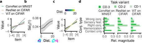
Figure 4: Behavior of networks trained on MNIST and CIFAR versions of compositional tasks. Shaded regions indicate mean $\pm$ two standard errors. a, Inferred values on symbolic addition (extrapolation, distance of zero between digits). b, $\text{Sal}_{2}(1)$ in an intermediate layer of the ConvNet, for different distances between digits. c, Inferred values for the extrapolation task and different distances between digits. d, For the networks trained on variants of context dependence, the inferred coefficients for different conjunction types (distance of 20px).

Context dependence. We then trained the ConvNets on an MNIST version of context dependence using 30,000 training samples and the ResNets and ViTs on a CIFAR-10 version of the task using 40,000 training samples. Again, their behavior was aligned with the kernel theory’s predictions, having better-than-chance accuracy on CD-1 and CD-2, but failing to generalize on CD-3. The additivity analysis revealed that this was due to a context-driven shortcut (Fig. 4d).

4.5 Feature learning can overcome the limitations of kernel models

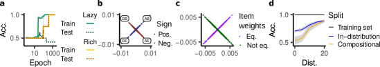
Figure 5: Feature learning enables generalization on transitive equivalence. a, Learning curves in the lazy and rich regime. b, The weights of the network in the subspace corresponding to one underlying XOR-task. c, Weights for the same unit are plotted against each other and colored by whether they correspond to equivalent items (purple) or non-equivalent items (green). d, Accuracy of a ConvNet trained on an MNIST version of transitive equivalence.

We proved above that compositionally structured kernel models do not generalize on non-additive tasks, including transitive equivalence. To see if feature learning can overcome this limitation, we trained ReLU networks through backpropagation on transitive equivalence, using a disentangled and uncorrelated input. By varying the initial weight magnitude, we either trained these networks in the kernel/lazy regime or the feature-learning/rich regime. Notably, when trained on symbolic addition and context dependence, the rich networks were well-described by a conjunction-wise additive model (Figs. 8 and 11). On transitive equivalence, however, while the kernel-regime models failed to generalize (as predicted by our theory), the rich networks generalized correctly (Fig. 5a).

To explain why this is the case, we leveraged the insight that rich neural networks are biased to learning weights with a low overall $\ell_{2}$-norm ([62, 61]; cf. [110]). In particular, a one-hidden-layer ReLU network tends to learn a sparse set of features [60, 61]. Transitive equivalence consists of multiple overlapping equality relations (e.g. $A=B\neq D=E$). Notably, ReLU networks such an XOR-type problem by specializing one unit to each conjunction ([111, 63, 112]; Fig. 5b). Further, their sparse inductive bias incentivizes ReLU networks to use identical units for overlapping conjunctions (e.g. $(A,B),(A,C)$, and $(B,C)$). This causes the unit to generalize to unseen item combinations (e.g. $(A,C)$), enabling the network to generalize. Importantly, our theoretical argument is corroborated by empirical simulations: each network unit has identical weights for equivalent items (Fig. 5c).

Thus, rich networks’ capacity for abstraction gives rise to an additional compositional motif, allowing them to generalize on transitive equivalence. In particular, our findings highlight that transitive equivalence and transitive ordering are solved by fundamentally different network motifs.

To see whether large-scale neural networks can also benefit from this feature-learning mechanism, we trained ConvNets on an MNIST version of transitive equivalence. The networks were trained for 150 epochs on 20,000 samples. We found that if the digits were presented with a distance of zero, the network did not generalize compositionally at all. However, with increasing distance, the network started to improve its compositional generalization (Fig. 5e), demonstrating that a convolutional network can benefit from this rich compositional motif.

5 Discussion

Humans often generalize to new situations by stitching together concepts and knowledge from prior experience. Despite the broad importance of this ability (both for cognitive science and machine learning), it has remained unclear under what conditions compositionally structured representations give rise to compositional generalization. Here we have taken a step toward formalizing this relationship by clarifying the full range of compositional motifs implemented by kernel models with categorical compositionally structured representations (“conjunction-wise additivity”). For conjunction-wise additive tasks, we analyzed how representational geometry and training data impact successful generalization on important compositional building blocks, validating our analysis for deep neural networks trained on natural image data. For non-additive tasks, our results immediately imply that kernel models are unable to generalize. We then analyzed how feature-learning mechanisms can overcome these limitations and demonstrated that deep networks benefit from the same mechanisms. Taken together, this suggests that conjunction-wise additivity provides a useful generalization class for understanding compositional generalization in neural networks and perhaps even humans.

Limitations. We considered tasks with a fixed number of input components and fixed output dimensionality and assumed that all input components are represented orthogonally, excluding continuously varying components such as position. Further, our theoretical analysis focused on kernel models with fixed representations (though we considered deep neural networks through empirical simulations). Future work could extend the presented theory beyond these assumptions, and could further explore the range of compositional motifs in other learning models (e.g. rich neural networks and modular networks) more systematically. Nevertheless, we believe that this work is an important step towards a comprehensive theory of compositional generalization, covering a broad range of tasks and highlighting several phenomena that might help us understand more complex models as well.

Appendix A Proof of Theorem 4.1

See 4.1

Proof.

Because $K$ is compositionally structured, its similarity $K(I,I^{\prime})$ only depends on the overlap $O(I,I^{\prime})\subseteq\{1,\dotsc,C\}$. We denote the similarity for inputs overlapping in $S\subseteq\{1,\dotsc,C\}$ by $\kappa_{S}$ and define the overlap in the training dataset as

$$\mathcal{D}_{S}(I):=\left\{I^{\prime}\in\mathcal{D}^{(\text{train})}|\forall_{c\in S}I_{c}=I^{\prime}_{c}\right\}.$$ (8)

The key idea is to decompose $\mathcal{D}^{(\text{train})}$ into these different overlaps in order to separate the sum into its components. However, by our definition, the datasets $\mathcal{D}_{S}(I)$ are not disjoint. Indeed, $S\subseteq S^{\prime}$ implies $\mathcal{D}_{S^{\prime}}(I)\subseteq\mathcal{D}_{S}(I)$ and in particular $\mathcal{D}_{\emptyset}(I)=\mathcal{D}^{(\text{train})}$. To adjust for this, we define $\delta_{S}$ as the similarity added by $\kappa_{S}$ to the similarity between conjunctions with one component fewer, recursively defining

$$\delta_{\emptyset}=\kappa_{\emptyset},\quad\delta_{S}=\kappa_{S}-\sum_{S^{\prime}\subsetneq S}\delta_{S^{\prime}}.$$ (9)

We then decompose

$$f(I)=\sum_{I^{\prime}\in\mathcal{D}^{(\text{train})}}a_{I^{\prime}}K(I,I^{\prime})=\sum_{S\subseteq\{1,\dotsc,C\}}\delta_{S}\sum_{I^{\prime}\in\mathcal{D}_{S}(I)}a_{I^{\prime}}.$$ (10)

This equality obtains because for each $I^{\prime}\in\mathcal{D}^{(\text{train})}$,

$$\sum_{S:I^{\prime}\in\mathcal{D}_{S}(I)}\delta_{S}=\delta_{O(I,I^{\prime})}+\sum_{S\subsetneq O(I,I^{\prime})}\delta_{S^{\prime}}=\kappa_{O(I,I^{\prime})}=K(I,I^{\prime}),$$ (11)

which is true by definition. We note that for $S\notin\mathcal{O}(I)$, $\mathcal{D}_{S}(I)=\emptyset$. Defining

$$f_{S}(I):=\delta_{S}\sum_{I^{\prime}\in\mathcal{D}_{S}(I)}a_{I^{\prime}},$$ (12)

proves the proposition. ∎

Appendix B Representational geometries across different deep neural network architectures

We computed the saliences by iteratively computing the representational similarities using the kernels derived in prior work [97, 98, 99, 100].

B.1 Proof of Proposition 4.3

See 4.3

Proof.

Note that the proof is a minor extension of Lemma S1.3 in [28]. We present it here in a self-contained manner. We consider a nonlinearity

$$\sigma(u):=A\min(u,0)+\max(u,0),\quad A\in[0,1).$$ (13)

By prior work, [97, 98, 99, 100],

$$\mathbb{E}_{w}\left[\phi({w}^{T}{h}^{(l)}(z))\phi({w}^{T}{h}^{(l)}(z^{\prime}))\right]=\sigma^{2}\|h^{(l)}(z)\|_{2}\|h^{(l)}(z^{\prime})\|_{2}k\left(\hat{h}^{(l)}(z)^{T}\hat{h}^{(l)}(z^{\prime})\right),$$ (14)

where

$$k(u)=\frac{(1-A)^{2}}{2\pi}\left(\sqrt{1-u^{2}}+(\pi-\cos^{-1}(u))u\right)+Au,$$ (15)

$\sigma^{2}$ is the variance of the sampled weights, and $\hat{h}=h/\|\hat{h}\|_{2}$.

This means that for any two inputs that have a certain similarity $u$, their similarity in the $L$-th layer is given by $k^{(L)}(u)$, where $k^{(L)}$ denotes the $L$-times application of $k$. Let distinct trials in the input have a similarity of $\kappa_{d}$ and let identical trials have a similarity of $\kappa_{i}$. Any set of trials with overlapping components will have a similarity $\kappa$, $\kappa_{d}<\kappa<\kappa_{i}$. We denote their corresponding similarity in the $L$-th layer by $\kappa_{i}^{(L)},\kappa_{d}^{(L)},\kappa^{(L)}$. Our goal is now to show that

$$\lim_{L\to\infty}s^{(L)}=0,\quad s^{(L)}:=\frac{\kappa^{(L)}-\kappa^{(L)}_{d}}{\kappa^{(L)}_{i}-\kappa^{(L)}_{d}}=0.$$ (16)

This implies directly that the salience of all partial conjunctions converges to zero, which in turn implies that the salience of the full conjunction converges to one.

(14) implies that $\kappa_{i}^{(L+1)}=\sigma^{2}\kappa_{i}^{(L)}k(1)=\sigma^{2}\kappa_{i}^{(L)}\tfrac{1+A^{2}}{2}$. Notably, all inputs have the same magnitude and therefore have the same magnitude through all layers; this is given by $\sqrt{\kappa_{i}^{(L)}}$. We can therefore denote

$$\kappa^{(L+1)}=\sigma^{2}\kappa_{i}^{(L)}k\left(\kappa^{(L)}/\kappa_{i}^{(L)}\right).$$ (17)

Thus,

$$s^{(L+1)}=\frac{k(\kappa^{(L)}/\kappa_{i}^{(L)})-k(\kappa_{d}^{(L)}/\kappa_{i}^{(L)})}{k(1)-k(\kappa_{d}^{(L)}/\kappa_{i}^{(L)})}$$ (18)

We thus define new normalized variables $\hat{\kappa}^{(L)}:=\kappa^{(L)}/\kappa_{i}^{(L)},\hat{\kappa}_{d}^{(L)}:=\kappa_{d}^{(L)}/\kappa_{i}^{(L)}$, i.e.

$$s^{(L)}=\frac{\hat{\kappa}^{(L)}-\hat{\kappa}^{(L)}_{d}}{1-\hat{\kappa}_{d}^{(L)}},$$ (19)

and therefore

$$\hat{\kappa}^{(L)}=(1-\hat{\kappa}_{d}^{(L)})s^{(L)}+\hat{\kappa}_{d}^{(L)}.$$ (20)

Note that $\hat{\kappa}^{(L+1)}=k(\hat{\kappa}^{(L)})/k(1)$ and $\hat{\kappa}_{d}^{(L+1)}=k^{(}\hat{\kappa}^{(L)}_{d})/k(1)$. We thus define

$$\tilde{k}(u):=\frac{k(u)}{k(1)}=u+\frac{\rho}{\pi}(\sqrt{1-u^{2}}-\cos^{-1}(u)u),\quad\rho:=\frac{(1-A)^{2}}{(1+A)^{2}}.$$ (21)

Note that

$$\tilde{k}^{\prime}(u)=1+\frac{\rho}{\pi}\left(-\frac{u}{\sqrt{1-u^{2}}}-\cos^{-1}(u)+\frac{u}{\sqrt{1-u^{2}}}\right)=1-\frac{\rho}{\pi}\cos^{-1}(u).$$ (22)

Note that $k(1)=1$ and as for all $0\leq u<1$, $\tilde{k}^{\prime}(u)<1$, this is the only fixed point and $\hat{\kappa}^{(L)},\hat{\kappa}_{d}^{(L)}\to\infty$. We can therefore define

$$s^{(L+1)}=\frac{\tilde{k}\left((1-\hat{\kappa}_{d}^{(L)})s^{(L)}+\hat{\kappa}_{d}^{(L)}\right)-\hat{\kappa}_{d}^{(L)}}{1-\kappa_{d}^{(L)}}.$$ (23)

We now determine the fixed mapping to this mapping assuming that $\hat{\kappa}_{d}^{(L)}$ is fixed at some value $d$, i.e.:

$$\begin{split}f(s,d)&=\frac{\tilde{k}((1-d)s+d)-\tilde{k}(d)}{1-\tilde{k}(d)}.\end{split}$$ (24)

$s=0$ is a fixed point. Further,

$$\frac{\partial f(s,d)}{\partial s}=\frac{(1-d)\tilde{k}^{\prime}((1-d)s+d)}{1-\tilde{k}(d)}=\frac{(1-d)(1-\tfrac{\rho}{\pi}\cos^{-1}((1-d)s+d)}{1-d-\tfrac{\rho}{\pi}(\sqrt{1-d^{2}}-\cos^{-1}(d)d)}.$$ (25)

We now prove that this for $0<s\leq\tfrac{1}{2}$, this derivative is smaller than 1. Specifically,

$$\begin{split}&(1-d)(1-\tfrac{\rho}{\pi}\cos^{-1}((1-d)s+d)=\\ &1-d-\tfrac{\rho}{\pi}(\sqrt{1-d^{2}}-\cos^{-1}(d)d)+\tfrac{\rho}{\pi}r(s,d),\end{split}$$ (26)

where the residual is given by

$$\begin{split}r(s,d):=(d-1)\cos^{-1}((1-d)s+d)+\sqrt{1-d^{2}}-d\cos^{-1}d.\end{split}$$ (27)

We now need to prove that $r(s,d)<0$. Note that $r(s,d)$ is monotonically increasing in $s$ and therefore

$$\begin{split}r(s,d)\leq r(\tfrac{1}{2},d)&=(d-1)\cos^{-1}(\tfrac{1}{2}+\tfrac{1}{2}d)+\sqrt{1-d^{2}}-d\cos^{-1}d<0,\end{split}$$ (28)

where we infer the latter inequality by visual inspection of the plot of this function. ∎

B.2 Extended analysis of representational salience

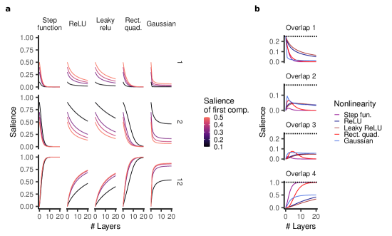
Figure 6: Extended analysis of overlap salience in random neural networks. a, Salience of the first component (1), the second component (2), and their conjunction (12), where we vary the two components’ saliences in the input. b, Salience for inputs with four components.

To complement Section 4.2, we analyze the impact of different magnitudes for different components. In particular, we consider a disentangled representation whose first component has a salience between $s\in[0.1,0.5]$ and whose second component accordingly has a salience $1-s$ (Fig. 6a). As becomes deeper, the more salient component (in this case component 2) increasingly dominates the representation. While the salience of the full conjunction still eventually converges to one for most nonlinearities, it takes longer to do so for a less balanced input representation. Further, for a Gaussian nonlinearity, an imbalanced representation actually decreases the limit salience the representation appears to be converging to for the full conjunction.

In Fig. 6, we plot the different saliences for an input with four components. Now the salience of overlap 2 and 3 both first increase and then decrease and, just like for inputs with three components (Fig. 2), a Gaussian and rectified quadratic nonlinearity yields a particularly high salience for these intermediate conjunctions. Notably, they appear to be trading off the salience of these conjunctions differently: the rectified quadratic nonlinearity more strongly emphasizes overlaps of three whereas the Gaussian nonlinearity more strongly emphasizes overlaps of two.

Appendix C Detailed methods

C.1 Models

Kernel model.

We fit the kernel models by hand-specifying the kernel and fitting either a support vector regression or classification using scikit-learn [113].

Rich and lazy ReLU networks.

All networks were trained with Pytorch and Pytorch Lightning [114]. We consider ReLU networks with one hidden layer and $H=1000$ units. We initialize by $\sigma\sqrt{2/H}$, considering $\sigma\in[10^{-6},1]$. In particular, when reporting results on rich networks (without further specification), we assume $\sigma=10^{-6}$. When reporting results on lazy network, we assume $\sigma=1$.

Convolutional neural networks.

We considered networks with four convolutional layers (kernel size is five, two layers have 32 filters, two have 64 filters) and two densely connected layers (with 512 and 1024 units). Each layer is followed by a ReLU nonlinearity, and the convolutional stage is followed by a max pooling operation. All weights are initialized with He initialization [115].

Residual neural networks.

We trained a residual neural network with eight blocks in total, two with 16, 32, 64, and 128 channels, respectively, using the Adam optimizer with a learning rate of $10^{-3}$ for 100 epochs.

Vision Transformers.

Finally, we trained a Vision Transformer (ViT) with six attention heads, 256 dimensions for both the attention layer and the MLP, and a depth of four, using Adam with a learning rate of $10^{-4}$ for 200 epochs.

Data augmentation.

We did not use data augmentation for MNIST. For CIFAR-10, we used a random flip and a random crop.

C.2 Reproducibility

Computational simulations.

We ran all computational simulations either on a CPU or on a single GPU. Each kernel experiment (total number: 53 experiments) ran within fifteen minutes, each rich network (total number: 450 experiments) and ConvNet experiment (total number: 600 experiments) took between one and two hours, and each ViT or ResNet experiment (total number: 140 experiments) took between five and ten hours. We used a computational cluster to run many of the experiments in parallel. As a rough estimate, the total experiments therefore required 900 hours of CPU computations and 2,600 hours of GPU computations.

Code repository.

The code required to reproduce all experiments can be found under https://github.com/sflippl/compositional-generalization. We additionally uploaded the repository including all simulated data to Zenodo (https://doi.org/10.5281/zenodo.11308156).

C.3 Additivity analysis

To analyze how well a conjunction-wise additive computation can describe network behavior, we considered as the set of possible features a concatenation of one-hot vectors coding for each possible conjunction. We then removed all features that are constant at zero on the training dataset and used linear regression to try and predict network behavior on both training and test set for all remaining features. The resulting $R^{2}$ defines the “additivity” of the network behavior (i.e. $R^{2}=1$ indicates full conjunction-wise additivity). Furthermore, we can use the inferred values assigned to these different conjunctions to compare kernel models, rich and lazy networks, and convolutional networks. Note that for the convolutional networks, we first average the model predictions across all different images instantiating a given compositional input.

Appendix D Compositional tasks

D.1 Symbolic addition

D.1.1 Proof of Proposition 4.4

See 4.4

Proof.

We split up the training data into

$$\mathcal{I}^{(1)}:=\{[w]|w\in\mathcal{W}\}^{2},$$ (29)

and

$$\mathcal{I}^{(2)} :=\bigcup_{w\in\mathcal{W}}\mathcal{I}^{(1,w)}\cup\mathcal{I}^{(2,w)},$$ (30)

$$\mathcal{I}^{(1,w)} :=\left\{([w],[v])|v\in\mathcal{V}\setminus\mathcal{W}\right\},\quad\mathcal{I}^{(2,w)}:=\left\{([v],[w])|v\in\mathcal{V}\setminus\mathcal{W}\right\}.$$ (31)

We denote the dual coefficient associated with each training point $([i],[j])$ by $a_{ij}\in\mathbb{R}$. Note that the problem is symmetric and therefore we know that $a_{ij}=a_{ji}$. We define a few summed coefficients:

$$b_{v}:=\sum_{w\in\mathcal{W}}a_{vw},\quad\overline{b}_{w}:=\sum_{v\in\mathcal{V}\setminus\mathcal{W}}a_{vw},\quad c_{w}:=\sum_{w^{\prime}\in\mathcal{W}}a_{ww^{\prime}},$$ (32)

$$b:=\sum_{v\in\mathcal{V}\setminus\mathcal{W}}b_{v}=\sum_{w\in\mathcal{W}}b_{w},\quad c:=\sum_{w\in\mathcal{W}}c_{w}.$$ (33)

Note that the sum over all dual coefficients is given by $2b+c$. Let $p:=|\mathcal{W}|$ and $q:=|\mathcal{V}|-|\mathcal{W}|$. Then, setting $\delta_{2}:=\kappa_{2}-\kappa_{0}$ and $\delta_{1}:=\kappa_{1}-\kappa_{0}$, the set of dual equations is given by

$$([w],[w^{\prime}])\in\mathcal{I}^{(1)}:\kappa_{0}(2b+c)+\delta_{1}(\overline{b}_{w}+\overline{b}_{w^{\prime}}+c_{w}+c_{w^{\prime}})+(\delta_{2}-2\delta_{1})a_{ww^{\prime}} =w+w^{\prime},$$ (34)

$$([w],[v])\in\mathcal{I}^{(1,w)}:\kappa_{0}(2b+c)+\delta_{1}(b_{v}+\overline{b}_{w}+c_{w})+(\delta_{2}-2\delta_{1})a_{wv} =w+v.$$ (35)

(Note that the equation corresponding to $([v],[w])$ is equivalent due to the problem’s symmetry.)

The prediction is given by

$$f([v_{1}],[v_{2}])=\kappa_{0}(2b+c)+\delta_{1}(b_{v_{1}}+b_{v_{2}}).$$ (36)

We now sum (35) over $w$ (setting $\overline{w}:=\sum_{w\in\mathcal{W}}w$):

$$\begin{split}\overline{w}+pv&=p\kappa_{0}(2b+c)+p\delta_{1}b_{v}+\delta_{1}(b+c)+(\delta_{2}-2\delta_{1})b_{v}\\ &=((p-2)\delta_{1}+\delta_{2})b_{v}+(2p\kappa_{0}+\delta_{1})b+(p\kappa_{0}+\delta_{1})c\end{split}$$ (37)

Thus,

$$\delta_{1}b_{v}=\frac{\delta_{1}p}{(p-2)\delta_{1}+\delta_{2}}v+\delta_{1}(\overline{w}-(2p\kappa_{0}+\delta_{1})b-(p\kappa_{0}+\delta_{1})c).$$ (38)

Thus, setting

$$m:=\frac{\delta_{1}p}{(p-2)\delta_{1}+\delta_{2}},\quad d:=2\delta_{1}(\overline{w}-(2p\kappa_{0}+\delta_{1})b-(p\kappa_{0}+\delta_{1})c)+\kappa_{0}(2b+c),$$ (39)

we can write

$$f([v_{1}],[v_{2}])=m(v_{1}+v_{2})+d.$$ (40)

To simplify $d$, we sum (34) over all $w,w^{\prime}$:

$$\begin{split}2p\overline{w}&=p^{2}\kappa_{0}(2b+c)+2p\delta_{1}(b+c)+(\delta_{2}-2\delta_{1})c\\ &=2p(p\kappa_{0}+\delta_{1})b+(p^{2}\kappa_{0}+2(p-1)\delta_{1}+\delta_{2})c.\end{split}$$ (41)

We further sum (37) over all $v$, setting $\overline{v}:=\sum_{v\in\mathcal{V}\setminus\mathcal{W}}v$:

$$((p+q-2)\delta_{1}+\delta_{2}+2pq\kappa_{0})b+q(p\kappa_{0}+\delta_{1})c=q\overline{w}+p\overline{v}.$$ (42)

We can now compute $b$ and $c$ from this system of equations and plug it into $d$.

Finally, $\overline{w}=\overline{v}=0$ immediately implies that $b=c=0$ and therefore $d=0$. ∎

D.1.2 Behavior of kernel models on other tasks

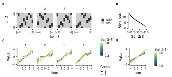
Figure 7: Kernel models on dispersed training sets. a, Four example training sets containing two random instances containing each item. b, Generalization loss as a function of the representation’s overlap salience. c,d, Inferred values for c) four example tasks and d) the average across fifty randomly drawn training sets.

To test whether the observed behavior was specific to the kinds of training sets investigated in Proposition 4.4 and the main text, we additionally considered dispersed, randomly generated training sets with two randomly drawn trials containing each item (Fig. 7a). We found that the generalized loss (averaged across all cases) increased roughly linearly with salience (Fig. 7b). For individual training sets, the inferred values were distorted in a complex, irregular manner (Fig. 7c). Further, because the training sets were no longer symmetric, the items took on different values when presented as the first or second component. On average, however, the inferred values were roughly proportional to their actual value and the factor of proportionality still decreased with salience (Fig. 7d).

D.1.3 Behavior of rich networks

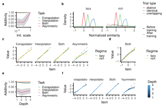
Figure 8: Behavior of rich networks on symbolic addition. a, Additivity as a function of initialization scale in networks with one hidden layer. b, Similarity between distinct, identical, and overlapping trials, before and after training in the lazy or rich regime. c, Inferred values in the lazy and rich regime for networks with one hidden layer. d, Zoomed-in inferred values for interpolation part of the task involving interpolation and extrapolation. e, Additivity as a function of the number of hidden layers. f, Inferred values for networks with different numbers of layers.

We first trained rich networks with one hidden layer on the different variants of symbolic addition. We found that they generally were highly additive ($R^{2}>0.992$, Fig. 8a). Fig. 8b confirms that the ReLU networks indeed change their representation in the rich regime: at initialization, the similarity between different trials is approximately clustered by whether those trials are distinct, overlapping, or identical. After lazy training, this remains unchanged, whereas after rich training, the similarities look entirely different. Finally, the inferred values look similar on extrapolation, but do not exhibit a memorization leak on interpolation (Fig. 8c). On the task involving both interpolation and extrapolation, the networks suffer from a memorization leak on the extrapolaton region but not the interpolation region (Fig. 8d). This indicates that rich networks tend to perform better at interpolation, unlike lazy networks which are not sensitive to this difference.

D.1.4 Behavior of deep networks

Next, we trained networks with one to four hidden layers, using $\sigma=0.1$. We found that the networks were generally highly additive ($R^{2}>0.985$, Fig. 8e) and inferred highly similar values. In particular, deeper networks also suffered from a memorization leak on extrapolation but not interpolation.

D.1.5 Behavior of vision models trained on MNIST and CIFAR-10

We now discuss in more detail the behavior of the different vision models.

First, we trained ConvNets on an MNIST version of symbolic addition for the different training sets. For all tasks, we found that compositional generalization was worse than in-distribution generalization (Fig. 9a) and become worse with smaller distance between the digits (i.e. higher conjunctivity). Further all networks were highly additive ($R^{2}>0.98$). Finally, the values inferred by the network were well consistent with the kernel theory: First, they were an affine function of the true item value for all training sets. Second, extrapolation was worse than interpolation and the task involving extrapolation and interpolation. Notably, interpolation and the task involving both yielded equally good values indicating that these networks may also not behave worse just based on extrapolation vs. interpolation. Further, smaller distance between digits (i.e. more conjunctive inputs) generally exacerbated the value misestimation. Finally, we also considered an asymmetric extrapolation task (“Asymmetric”), which trained on all trials containing an item $[-4]$. Consistent with our theory, we found that this resulted in an affine distortion in values.

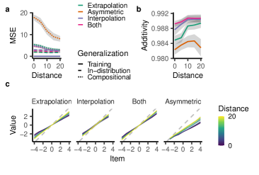
Figure 9: Behavior of ConvNets trained on MNIST versions of symbolic addition. a, Mean squared error for different training sets and different evaluation sets. b, Additivity on the different tasks. c, Inferred values.

We then trained a ResNet and a ViT on a CIFAR-10 version of the task. We found that the error on the compositional test dataset was consistently higher than on in-distribution generalization (Fig. 10a). Further, similarly to the ConvNets trained on MNIST, it was particularly high on the asymmetric training set. Notably, the additivity of all of these models was reasonably high ($R^{2}>0.93$, Fig. 10b). Finally, we found that the models all inferred values that were distorted in a roughly affine manner (Fig. 10c).

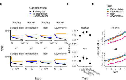
Figure 10: Behavior of ResNets and ViTs on CIFAR versions of symbolic addition. a, Mean squared error over training. b, Additivity. c, Inferred values for the different tasks.

D.2 Context dependence

D.2.1 General task definition

We consider inputs with three components, $(z_{\text{co}},z_{f1},z_{f2})$. We assume that $z_{\text{co}}\in C_{1}\cup C_{2}$, where $C_{1}$ is the set of possible contexts under which $z_{f1}$ is relevant and $C_{2}$ is the set of possible contexts under which $z_{f2}$ is relevant. We further assume that there are decision functions $d_{1}(z_{f1}),d_{2}(z_{f2})\in\mathbb{R}$. (For example, in the example in the main text, these function map three features to the first category (i.e. $y=-1$) and three features to the second category (i.e. $y=1$).) The target is then given by

$$y(z_{\text{co}},z_{f1},z_{f2})=\begin{cases}d_{1}(z_{f1})&\text{ if }z_{\text{co}}\in C_{1},\\ d_{2}(z_{f2})&\text{ if }z_{\text{co}}\in C_{2}.\end{cases}$$ (43)

Note that in the main text, we consider $C_{1}=\{1\}$, $C_{2}=\{2\}$, and six possible values for $z_{f1},z_{f2}$, where the decision function maps three onto $1$ and three onto $-1$.

D.2.2 Novel stimulus compositions are conjunction-wise additive

If the test set consists in novel combinations of stimuli, this is a conjunction-wise additive computation. Namely, suppose that for all test inputs $(z_{\text{co}},z_{f1},z_{f2})$, the two features have never been observed in conjunction, but both $(z_{\text{co}},z_{f1})$ and $(z_{\text{co}},z_{f2})$ have been. (This includes the case considered in the main text.) In this case, we can define functions $f_{12}$ and $f_{13}$ to implement the appropriate mapping:

$$f_{12}(z_{\text{co}},z_{f1}) :=\begin{cases}d_{1}(z_{f1})&\text{ if }z_{\text{co}}\in C_{1},\\ 0&\text{ if }z_{\text{co}}\in C_{2},\end{cases}\quad f_{13}(z_{\text{co}},z_{f2}):=\begin{cases}0&\text{ if }z_{\text{co}}\in C_{1},\\ d_{2}(z_{f2})&\text{ if }z_{\text{co}}\in C_{2},\end{cases}$$ (44)

$$f(z_{\text{co}},z_{f1},z_{f2}) =f_{12}(z_{\text{co}},z_{f1})+f_{13}(z_{\text{co}},z_{f2}).$$ (45)

D.2.3 Novel rule compositions are not conjunction-wise additive

We could also imagine an alternative generalization rule in a task where there are multiple components indicating the same context: $C_{1}=\{\text{co}_{1},\text{co}_{2}\}$ and $C_{2}=\{\text{co}_{3},\text{co}_{4}\}$. We then leave out certain features with certain contexts. For example, suppose we had never seen two values for $z_{f1}$ and $z_{f2}$ in conjunction with $z_{\text{co}}\in\{\text{co}_{2},\text{co}_{4}\}$. In principle, if the model understood that $z_{\text{co}}=\text{co}_{1},\text{co}_{2}$ (and $z_{\text{co}}=\text{co}_{3},\text{co}4$ resp.) signify the same context (i.e. learned to abstract the context from the context cue), it could generalize successfully as it had observed these features in conjunction with $z_{\text{co}}=\text{co}_{1},\text{co}_{3}$. However, the conjunction-wise additive mapping depends on having observed each context in conjunction with each feature and this task is therefore non-additive.

D.2.4 Coefficient groups

In Fig. 3d, we grouped the inferred coefficients into categories. We here explain these categories:

• Right conj.: This is the correct conjunction the model should use to solve the task, i.e. between $z_{\text{co}}=\text{co}_{1}$ and $z_{f1}$ and between $z_{\text{co}}=\text{co}_{2}$ and $z_{f2}$.

• Wrong conj.: This is the incorrect conjunction between context and feature, i.e. between $z_{\text{co}}=\text{co}_{1}$ and $z_{f2}$ and between $z_{\text{co}}=\text{co}_{2}$ and $z_{f1}$.

• Sensory feat.: This is any conjunction involving sensory features, i.e. $z_{f1},z_{f2},(z_{f1},z_{f2})$.

• Context only: This is the component $z_{\text{co}}$ by itself.

• Memorization: This is the full conjunction of all three components $(z_{\text{co}},z_{f1},z_{f2})$.

We then compute the average absolute magnitude within each of these groups in order to determine their overall relevance to model behavior.

D.2.5 Rich networks

We find that rich networks generalize consistently on CD-1 and CD-2 but not CD-3. They are also perfectly conjunction-wise additive and fail due to a context shortcut (Fig. 11).

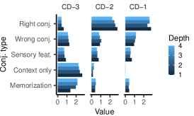
Figure 11: Inferred values for different conjunctive groups on context dependence.

D.2.6 Deep neural networks trained on vision data

We found that convolutional neural networks trained on MNIST successfully generalized on CD-1 and CD-2, but not CD-3 (Fig. 12). For smaller distances between digits, the models tended to generalize worse on CD-1 and CD-2 and gradually reverted to chance accuracy (i.e. 0.5) for CD-3. Further, the networks were generally highly additive ($R^{2}>0.95$), but became worse for lower distance (Fig. 12b). Finally, across all distances, they had a high magnitude associated with the context cue, though this magnitude decreased for small distances — consistent with the accuracy of the network increasing from below chance to chance level (Fig. 12c).

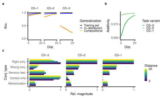
Figure 12: Performance of convolutional neural networks trained on an MNIST version of context dependence. For different distances and training sets, we plot a, the accuracy on different splits, b, the additivity of the networks, and c, the magnitude of the different inferred coefficients.

Finally, we considered ResNets and ViTs trained on a CIFAR version of the task. We found that they generally performed above chance for CD-2 and CD-1, but below chance for CD-3 (Fig. 13a). Further, their additivity was generally high for ResNets ($R^{2}>0.95$) and slightly lower for ViTs ($R^{2}>0.9$) (Fig. 13b) and both networks had a large magnitude associated with the context cue for CD-3, but not CD-2 or CD-1 (Fig. 13c).

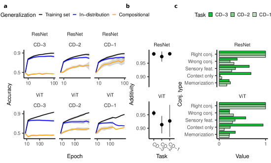
Figure 13: Performance of ResNets and ViTs trained on a CIFAR version of context dependence. We plot a, their accuracy on different splits over training, b, the additivity of the networks, and c, the magnitude of the different inferred coefficients.

D.3 Transitive equivalence

We additionally trained ReLU networks of various depth on the transitive equivalence (using $\sigma=0.1$ as initialization magnitude). We consistently found that they were able to generalize to the test set (Fig. 14).

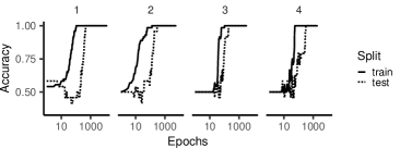
Figure 14: Performance of networks with 100 hidden units per layer and varying depth on transitive equivalence. We used an initialization constant $\sigma=0.1$.

D.4 Invariance and partial exposure

We consider invariance and partial exposure as simple case studies for the memorization leak and shortcut distortion. In both cases, the input consists of two components and the mapping only depends on the first (Fig. 15a). In the invariance case, we don’t see the second component vary at all, in the partial exposure case, we see one instance of the second component. Note that the partial exposure task has previously been studied in the context of network generalization [81, 82].

To understand the impact of different representational saliences, we consider the generalization margin $m:=y\hat{y}$ on the test set, where $y$ is the ground-truth label and $\hat{y}$ is the model’s estimate. Because we consider support vector machines, the margin on the training set is one; a smaller margin on the test set indicates worse performance. We determined a mathematical formula for the margins as a function of $\text{Sal}_{2}(1)$. Below we first describe its implications and then how we derived this.

Invariance suffers from a memorization leak.

On invariance, we find that the model’s test margin is expressed as $m=\tfrac{\text{Sal}_{2}(1)}{1-\text{Sal}_{2}(1)}$. This means that for a fully compositional representation ($\hat{\kappa}_{1}=0.5$), its training and test margins are both one. However, as $\hat{\kappa}_{1}$ decreases, the model increasingly memorizes the training set, resulting in a decreased margin (Fig. 15b).

Shortcut distortion.

On the partial exposure task, if the model used item 1 to solve the task, it would get two out of three training examples correct and could memorize the last data point. This is a statistical shortcut and we find that norm minimization (just as for context dependence) ends up partially relying on this strategy as this decreases the $\ell_{2}$-norm of the readout weights. As a result, the test margin for the partial exposure task decreases even more strongly as a function of $\text{Sal}_{2}(1)$: $m=\tfrac{2\text{Sal}_{2}(1)^{2}}{1-2\text{Sal}_{2}(1)^{2}}$ (where we assume that the similarity between identical trials is one and the similarity between distinct trials is zero) (Fig. 15b).

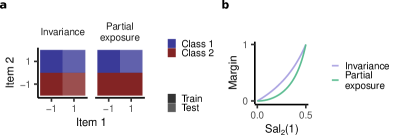
Figure 15: a, Schema for invariance and partial exposure. b, Generalization margin for the two tasks.

Derivations.

We analytically compute the kernel models’ test set prediction on the invariance task. The training set is given by $\{(-1,-1),(-1,1)\}$ and its kernel is therefore

$$K=\begin{pmatrix}\kappa_{2}&\kappa_{1}\\ \kappa_{1}&\kappa_{2}\end{pmatrix},$$ (46)

where $\kappa_{2}$ is the similarity between identical trials and $\kappa_{1}$ is the similarity between overlapping trials. Hence, the dual coefficients are given by

$$a=K^{-1}\begin{pmatrix}1\\ -1\end{pmatrix}=\frac{1}{\kappa_{2}^{2}-\kappa_{1}^{2}}\begin{pmatrix}\kappa_{2}&-\kappa_{1}\\ -\kappa_{1}&\kappa_{2}\end{pmatrix}\begin{pmatrix}1\\ -1\end{pmatrix}=\frac{1}{\kappa_{2}^{2}-\kappa_{1}^{2}}\begin{pmatrix}\kappa_{2}+\kappa_{1}\\ -(\kappa_{2}+\kappa_{1})\end{pmatrix}.$$ (47)

The test set is given by $\{(1,-1),(1,1)\}$ and its kernel with respect to the training set is therefore

$$\tilde{K}=\begin{pmatrix}\kappa_{1}&\kappa_{0}\\ \kappa_{0}&\kappa_{1}\end{pmatrix},$$ (48)

where $\kappa_{0}$ is the similarity between distinct trials. Hence the test set predictions are given by

$$\hat{y}=\tilde{K}a=\frac{1}{\kappa_{2}^{2}-\kappa_{1}^{2}}\begin{pmatrix}(\kappa_{2}+\kappa_{1})(\kappa_{1}-\kappa_{0})\\ -(\kappa_{2}+\kappa_{1})(\kappa_{1}-\kappa_{0}).\end{pmatrix}$$ (49)

As the ground truth labels are $y=\{1,-1\}$, the margin $m=y\hat{y}$ is identical for both test set points:

$$m=\frac{(\kappa_{2}+\kappa_{1})(\kappa_{1}-\kappa_{0})}{\kappa_{2}^{2}-\kappa_{1}^{2}}=\frac{\kappa_{1}-\kappa_{0}}{\kappa_{2}-\kappa_{1}}=\frac{(\kappa_{2}-\kappa_{0})\text{Sal}_{2}(1)}{(\kappa_{2}-\kappa_{0})-(\kappa_{1}-\kappa_{0})}=\frac{\text{Sal}_{2}(1)}{1-\text{Sal}_{2}(1)}.$$ (50)

For partial exposure, the training set is given by $\{(-1,-1),(-1,1),(1,-1)\}$ and its kernel is therefore

$$K=\begin{pmatrix}\kappa_{2}&\kappa_{1}&\kappa_{1}\\ \kappa_{1}&\kappa_{2}&\kappa_{0}\\ \kappa_{1}&\kappa_{0}&\kappa_{2}\end{pmatrix}.$$ (51)

The test set is given by $\{(1,1)\}$ and the test set kernel is therefore

$$\tilde{K}=\begin{pmatrix}\kappa_{0}&\kappa_{1}&\kappa_{1}\end{pmatrix}$$ (52)

The margin is therefore given by

$$m=y\hat{y}=-\hat{y}=-\tilde{K}K^{-1}\begin{pmatrix}1\\ -1\\ 1\end{pmatrix}.$$ (53)

We solve this equation for the special case where $\kappa_{0}=0$ and $\kappa_{1}=1$ using Mathematica and find that

$$m=\frac{2\text{Sal}_{2}(1)^{2}}{1-2\text{Sal}_{2}(1)^{2}}.$$ (54)

D.5 Other mathematical operations

We could consider mathematical operations other than addition as well, considering unobserved assigned values $v_{1}[I_{1}]$ and $v_{2}[I_{2}]$ together with some composition function $C(v_{1}[I_{1}],v_{2}[I_{2}])$. This task will only be additive if the composition function is additive (e.g. if it is subtraction). If it is, e.g. multiplication, division, or exponentiation, the task will be non-additive.

D.6 Logical operations

In this task, inputs with two components are presented. Each component $I_{c}$ has an unobserved truth value $T[I_{c}]$ associated with it and the target is some logical operation over these two truth values, for example AND: $T[I_{1}]\wedge T[I_{2}]$. After inferring the truth value of each component, the model could generalize towards novel item combinations. As long as the logical operation is additive (e.g. AND, OR, NEITHER, $\dotsc$), this is an additive task. If the logical operation is non-additive (e.g. XOR), this would be a non-additive task. Indeed, this case would correspond to the transitive equivalence task.

D.7 Transitive ordering

Transitive ordering is a popular task in cognitive science (often called transitive inference, [116]). Here the subject is presented with two items $I_{1}$, $I_{2}$ drawn from an unobserved hierarchy $>$. It should then categorize whether $I_{1}>I_{2}$ or $I_{2}>I_{1}$. Crucially, this task can be solved by assigning a rank $r(I_{c})$ to each item and computing the response as $f(I)=r(I_{1})-r(I_{2})$ [28]. It is therefore additive, in contrast to transitive equivalence. This is also the case if we assume that there are multiple such hierarchies (e.g. $a_{1}>\dotsc,a_{5}$ and $b_{1}>\dotsc,b_{5}$). In this case, the model would generalize to comparisons between these different hierarchies as well.

References

- [1] Brenden M. Lake, Tomer D. Ullman, Joshua B. Tenenbaum and Samuel J. Gershman “Building machines that learn and think like people” Publisher: Cambridge University Press In Behavioral and Brain Sciences 40, 2017, pp. e253 DOI: 10.1017/S0140525X16001837
- [2] Steven M. Frankland and Joshua D. Greene “Concepts and Compositionality: In Search of the Brain’s Language of Thought” _eprint: https://doi.org/10.1146/annurev-psych-122216-011829 In Annual Review of Psychology 71.1, 2020, pp. 273–303 DOI: 10.1146/annurev-psych-122216-011829
- [3] Jerry A. Fodor and Zenon W. Pylyshyn “Connectionism and cognitive architecture: A critical analysis” In Cognition 28.1, 1988, pp. 3–71 DOI: 10.1016/0010-0277(88)90031-5
- [4] Peter W. Battaglia et al. “Relational inductive biases, deep learning, and graph networks” arXiv:1806.01261 [cs, stat] arXiv, 2018 DOI: 10.48550/arXiv.1806.01261
- [5] Brenden Lake and Marco Baroni “Generalization without systematicity: 35th International Conference on Machine Learning, ICML 2018” Publisher: International Machine Learning Society (IMLS) In 35th International Conference on Machine Learning, ICML 2018, 35th International Conference on Machine Learning, ICML 2018, 2018, pp. 4487–4499 URL: http://www.scopus.com/inward/record.url?scp=85057241154&partnerID=8YFLogxK
- [6] Dieuwke Hupkes, Verna Dankers, Mathijs Mul and Elia Bruni “Compositionality Decomposed: How do Neural Networks Generalise?” In Journal of Artificial Intelligence Research 67, 2020, pp. 757–795 DOI: 10.1613/jair.1.11674
- [7] Daniel Keysers et al. “Measuring Compositional Generalization: A Comprehensive Method on Realistic Data” arXiv:1912.09713 [cs, stat] arXiv, 2020 DOI: 10.48550/arXiv.1912.09713
- [8] Geoffrey E. Hinton, Alex Krizhevsky and Sida D. Wang “Transforming Auto-Encoders” In Artificial Neural Networks and Machine Learning – ICANN 2011 Berlin, Heidelberg: Springer, 2011, pp. 44–51 DOI: 10.1007/978-3-642-21735-7_6
- [9] Yoshua Bengio, Aaron Courville and Pascal Vincent “Representation learning: A review and new perspectives” Publisher: IEEE In IEEE transactions on pattern analysis and machine intelligence 35.8, 2013, pp. 1798–1828
- [10] Irina Higgins et al. “beta-VAE: Learning Basic Visual Concepts with a Constrained Variational Framework” In International Conference on Learning Representations, 2017 URL: https://openreview.net/forum?id=Sy2fzU9gl
- [11] Francesco Locatello et al. “Challenging common assumptions in the unsupervised learning of disentangled representations” In international conference on machine learning PMLR, 2019, pp. 4114–4124
- [12] Babak Esmaeili et al. “Structured Disentangled Representations” ISSN: 2640-3498 In Proceedings of the Twenty-Second International Conference on Artificial Intelligence and Statistics PMLR, 2019, pp. 2525–2534 URL: https://proceedings.mlr.press/v89/esmaeili19a.html
- [13] Frederik Träuble et al. “On Disentangled Representations Learned from Correlated Data” ISSN: 2640-3498 In Proceedings of the 38th International Conference on Machine Learning PMLR, 2021, pp. 10401–10412 URL: https://proceedings.mlr.press/v139/trauble21a.html
- [14] James C.. Whittington, Will Dorrell, Surya Ganguli and Timothy Behrens “Disentanglement with Biological Constraints: A Theory of Functional Cell Types” In The Eleventh International Conference on Learning Representations, 2023 URL: https://openreview.net/forum?id=9Z_GfhZnGH
- [15] Pavel Tokmakov, Yu-Xiong Wang and Martial Hebert “Learning Compositional Representations for Few-Shot Recognition”, 2019, pp. 6372–6381 URL: https://openaccess.thecvf.com/content_ICCV_2019/html/Tokmakov_Learning_Compositional_Representations_for_Few-Shot_Recognition_ICCV_2019_paper.html
- [16] Sjoerd Steenkiste, Francesco Locatello, Jürgen Schmidhuber and Olivier Bachem “Are Disentangled Representations Helpful for Abstract Visual Reasoning?” In Advances in Neural Information Processing Systems 32 Curran Associates, Inc., 2019 URL: https://proceedings.neurips.cc/paper_files/paper/2019/hash/bc3c4a6331a8a9950945a1aa8c95ab8a-Abstract.html
- [17] James C.. Whittington et al. “Constellation: Learning relational abstractions over objects for compositional imagination” arXiv:2107.11153 [cs, stat] arXiv, 2021 DOI: 10.48550/arXiv.2107.11153
- [18] Milton Llera Montero et al. “The role of Disentanglement in Generalisation” In International Conference on Learning Representations, 2021 URL: https://openreview.net/forum?id=qbH974jKUVy
- [19] Lukas Schott et al. “Visual Representation Learning Does Not Generalize Strongly Within the Same Domain” In International Conference on Learning Representations, 2022 URL: https://openreview.net/forum?id=9RUHPlladgh
- [20] Zhenlin Xu, Marc Niethammer and Colin A Raffel “Compositional generalization in unsupervised compositional representation learning: A study on disentanglement and emergent language” In Advances in Neural Information Processing Systems 35, 2022, pp. 25074–25087
- [21] Arthur Jacot, Franck Gabriel and Clément Hongler “Neural tangent kernel: Convergence and generalization in neural networks” In Advances in neural information processing systems 31, 2018
- [22] Lénaïc Chizat, Edouard Oyallon and Francis Bach “On Lazy Training in Differentiable Programming” In Advances in Neural Information Processing Systems 32 Curran Associates, Inc., 2019 URL: https://proceedings.neurips.cc/paper/2019/hash/ae614c557843b1df326cb29c57225459-Abstract.html
- [23] Frank Jäkel, Bernhard Schölkopf and Felix A Wichmann “Generalization and similarity in exemplar models of categorization: Insights from machine learning” Publisher: Springer In Psychonomic Bulletin & Review 15, 2008, pp. 256–271
- [24] Frank Jäkel, Bernhard Schölkopf and Felix A. Wichmann “Does Cognitive Science Need Kernels?” Publisher: Elsevier In Trends in Cognitive Sciences 13.9, 2009, pp. 381–388 DOI: 10.1016/j.tics.2009.06.002
- [25] Abdulkadir Canatar, Blake Bordelon and Cengiz Pehlevan “Spectral bias and task-model alignment explain generalization in kernel regression and infinitely wide neural networks” Publisher: Nature Publishing Group In Nature Communications 12.1, 2021, pp. 2914 DOI: 10.1038/s41467-021-23103-1
- [26] Abdulkadir Canatar, Blake Bordelon and Cengiz Pehlevan “Out-of-Distribution Generalization in Kernel Regression” In Advances in Neural Information Processing Systems 34 Curran Associates, Inc., 2021, pp. 12600–12612 URL: https://proceedings.neurips.cc/paper/2021/hash/691dcb1d65f31967a874d18383b9da75-Abstract.html
- [27] Emmanuel Abbe, Samy Bengio, Aryo Lotfi and Kevin Rizk “Generalization on the Unseen, Logic Reasoning and Degree Curriculum”, 2023 URL: https://openreview.net/forum?id=3dqwXb1te4
- [28] Samuel Lippl et al. “A mathematical theory of relational generalization in transitive inference” Pages: 2023.08.22.554287 Section: New Results bioRxiv, 2024 DOI: 10.1101/2023.08.22.554287
- [29] Brenden M. Lake, Ruslan Salakhutdinov and Joshua B. Tenenbaum “Human-level concept learning through probabilistic program induction” Publisher: American Association for the Advancement of Science In Science 350.6266, 2015, pp. 1332–1338 DOI: 10.1126/science.aab3050
- [30] Justin Johnson et al. “CLEVR: A Diagnostic Dataset for Compositional Language and Elementary Visual Reasoning”, 2017, pp. 2901–2910 URL: https://openaccess.thecvf.com/content_cvpr_2017/html/Johnson_CLEVR_A_Diagnostic_CVPR_2017_paper.html
- [31] Kenneth Marino, Mohammad Rastegari, Ali Farhadi and Roozbeh Mottaghi “OK-VQA: A Visual Question Answering Benchmark Requiring External Knowledge”, 2019, pp. 3195–3204 URL: https://openaccess.thecvf.com/content_CVPR_2019/html/Marino_OK-VQA_A_Visual_Question_Answering_Benchmark_Requiring_External_Knowledge_CVPR_2019_paper.html
- [32] Philipp Schwartenbeck et al. “Generative replay underlies compositional inference in the hippocampal-prefrontal circuit” Place: United States In Cell, 2023 URL: https://doi.org/10.1016/j.cell.2023.09.004
- [33] Yanli Zhou, Reuben Feinman and Brenden M. Lake “Compositional diversity in visual concept learning” In Cognition 244, 2024, pp. 105711 DOI: 10.1016/j.cognition.2023.105711
- [34] Takuya Ito et al. “Compositional generalization through abstract representations in human and artificial neural networks” arXiv:2209.07431 [q-bio] arXiv, 2022 DOI: 10.48550/arXiv.2209.07431
- [35] Mustafa Abdool, Andrew J Nam and James L McClelland “Continual learning and out of distribution generalization in a systematic reasoning task” In MATH-AI: The 3rd Workshop on Mathematical Reasoning and AI at NeurIPS 23, 2023
- [36] Maya Okawa, Ekdeep Singh Lubana, Robert P. Dick and Hidenori Tanaka “Compositional Abilities Emerge Multiplicatively: Exploring Diffusion Models on a Synthetic Task”, 2023 URL: https://openreview.net/forum?id=ZXH8KUgFx3
- [37] Allan Zhou, Vikash Kumar, Chelsea Finn and Aravind Rajeswaran “Policy Architectures for Compositional Generalization in Control” arXiv:2203.05960 [cs] arXiv, 2022 DOI: 10.48550/arXiv.2203.05960
- [38] Aarohi Srivastava et al. “Beyond the Imitation Game: Quantifying and extrapolating the capabilities of language models” arXiv:2206.04615 [cs, stat] arXiv, 2023 DOI: 10.48550/arXiv.2206.04615
- [39] Martha Lewis et al. “Does CLIP Bind Concepts? Probing Compositionality in Large Image Models” arXiv:2212.10537 [cs] arXiv, 2023 DOI: 10.48550/arXiv.2212.10537
- [40] Colin G. West “Advances in apparent conceptual physics reasoning in GPT-4” Publication Title: arXiv e-prints ADS Bibcode: 2023arXiv230317012W, 2023 DOI: 10.48550/arXiv.2303.17012
- [41] Zixian Ma et al. “CREPE: Can Vision-Language Foundation Models Reason Compositionally?”, 2023, pp. 10910–10921 URL: https://openaccess.thecvf.com/content/CVPR2023/html/Ma_CREPE_Can_Vision-Language_Foundation_Models_Reason_Compositionally_CVPR_2023_paper.html
- [42] Jiaao Chen et al. “Skills-in-Context Prompting: Unlocking Compositionality in Large Language Models” arXiv:2308.00304 [cs] arXiv, 2023 DOI: 10.48550/arXiv.2308.00304
- [43] Brenden M. Lake, Tal Linzen and Marco Baroni “Human few-shot learning of compositional instructions: 41st Annual Meeting of the Cognitive Science Society: Creativity + Cognition + Computation, CogSci 2019” Publisher: The Cognitive Science Society In Proceedings of the 41st Annual Meeting of the Cognitive Science Society, Proceedings of the 41st Annual Meeting of the Cognitive Science Society: Creativity + Cognition + Computation, CogSci 2019, 2019, pp. 611–617 URL: http://www.scopus.com/inward/record.url?scp=85091234961&partnerID=8YFLogxK
- [44] Eric Mitchell, Chelsea Finn and Chris Manning “Challenges of acquiring compositional inductive biases via meta-learning” In AAAI Workshop on Meta-Learning and MetaDL Challenge PMLR, 2021, pp. 138–148
- [45] Sreejan Kumar et al. “Meta-Learning of Structured Task Distributions in Humans and Machines” In International Conference on Learning Representations, 2021 URL: https://openreview.net/forum?id=--gvHfE3Xf5
- [46] Bin Wu et al. “Adaptive compositional continual meta-learning” In International Conference on Machine Learning PMLR, 2023, pp. 37358–37378
- [47] Brenden M. Lake and Marco Baroni “Human-like systematic generalization through a meta-learning neural network” Publisher: Nature Publishing Group In Nature 623.7985, 2023, pp. 115–121 DOI: 10.1038/s41586-023-06668-3
- [48] Jacob Andreas, Marcus Rohrbach, Trevor Darrell and Dan Klein “Neural Module Networks” arXiv:1511.02799 [cs] arXiv, 2017 DOI: 10.48550/arXiv.1511.02799
- [49] Dzmitry Bahdanau et al. “Systematic Generalization: What Is Required and Can It Be Learned?” arXiv:1811.12889 [cs] arXiv, 2019 DOI: 10.48550/arXiv.1811.12889
- [50] Sarthak Mittal, Yoshua Bengio and Guillaume Lajoie “Is a Modular Architecture Enough?” In Advances in Neural Information Processing Systems 35, 2022, pp. 28747–28760 URL: https://proceedings.neurips.cc/paper_files/paper/2022/hash/b8d1d741f137d9b6ac4f3c1683791e4a-Abstract-Conference.html
- [51] Devon Jarvis, Richard Klein, Benjamin Rosman and Andrew M. Saxe “On The Specialization of Neural Modules” In The Eleventh International Conference on Learning Representations, 2023 URL: https://openreview.net/forum?id=Fh97BDaR6I
- [52] Simon Schug et al. “Discovering modular solutions that generalize compositionally” arXiv:2312.15001 [cs] arXiv, 2024 DOI: 10.48550/arXiv.2312.15001
- [53] Sebastien Lachapelle, Divyat Mahajan, Ioannis Mitliagkas and Simon Lacoste-Julien “Additive Decoders for Latent Variables Identification and Cartesian-Product Extrapolation”, 2023 URL: https://openreview.net/forum?id=R6KJN1AUAR
- [54] Thaddäus Wiedemer, Prasanna Mayilvahanan, Matthias Bethge and Wieland Brendel “Compositional Generalization from First Principles” In Advances in Neural Information Processing Systems 36, 2023, pp. 6941–6960 URL: https://proceedings.neurips.cc/paper_files/paper/2023/hash/15f6a10899f557ce53fe39939af6f930-Abstract-Conference.html
- [55] Tomas Mikolov et al. “Distributed Representations of Words and Phrases and their Compositionality” In Advances in Neural Information Processing Systems 26 Curran Associates, Inc., 2013 URL: https://proceedings.neurips.cc/paper/2013/hash/9aa42b31882ec039965f3c4923ce901b-Abstract.html
- [56] Masahiro Naito, Sho Yokoi, Geewook Kim and Hidetoshi Shimodaira “Revisiting Additive Compositionality: AND, OR and NOT Operations with Word Embeddings” In arXiv.org, 2021 URL: https://arxiv.org/abs/2105.08585v2
- [57] Maria C. Alvarado and Jerry W. Rudy “Some properties of configural learning: An investigation of the transverse-patterning problem” Place: US Publisher: American Psychological Association In Journal of Experimental Psychology: Animal Behavior Processes 18.2, 1992, pp. 145–153 DOI: 10.1037/0097-7403.18.2.145
- [58] Chris I Baker, Marlene Behrmann and Carl R Olson “Impact of learning on representation of parts and wholes in monkey inferotemporal cortex” Publisher: Nature Publishing Group US New York In Nature neuroscience 5.11, 2002, pp. 1210–1216
- [59] Blake Woodworth et al. “Kernel and rich regimes in overparametrized models” In Conference on Learning Theory PMLR, 2020, pp. 3635–3673
- [60] Pedro Savarese, Itay Evron, Daniel Soudry and Nathan Srebro “How do infinite width bounded norm networks look in function space?” In Proceedings of the Thirty-Second Conference on Learning Theory 99, Proceedings of Machine Learning Research PMLR, 2019, pp. 2667–2690 URL: https://proceedings.mlr.press/v99/savarese19a.html
- [61] Lénaïc Chizat and Francis Bach “Implicit Bias of Gradient Descent for Wide Two-layer Neural Networks Trained with the Logistic Loss” ISSN: 2640-3498 In Proceedings of Thirty Third Conference on Learning Theory PMLR, 2020, pp. 1305–1338 URL: https://proceedings.mlr.press/v125/chizat20a.html
- [62] Kaifeng Lyu and Jian Li “Gradient Descent Maximizes the Margin of Homogeneous Neural Networks” In International Conference on Learning Representations, 2020 URL: https://openreview.net/forum?id=SJeLIgBKPS
- [63] Andrew Saxe, Shagun Sodhani and Sam Jay Lewallen “The Neural Race Reduction: Dynamics of Abstraction in Gated Networks” ISSN: 2640-3498 In Proceedings of the 39th International Conference on Machine Learning PMLR, 2022, pp. 19287–19309 URL: https://proceedings.mlr.press/v162/saxe22a.html
- [64] Yuhan Helena Liu et al. “How connectivity structure shapes rich and lazy learning in neural circuits” In arXiv preprint arXiv:2310.08513, 2023
- [65] Clémentine CJ Dominé, Lukas Braun, James E Fitzgerald and Andrew M Saxe “Exact learning dynamics of deep linear networks with prior knowledge” Publisher: IOP Publishing In Journal of Statistical Mechanics: Theory and Experiment 2023.11, 2023, pp. 114004
- [66] Stanislav Fort et al. “Deep learning versus kernel learning: an empirical study of loss landscape geometry and the time evolution of the Neural Tangent Kernel” In Advances in Neural Information Processing Systems 33 Curran Associates, Inc., 2020, pp. 5850–5861 URL: https://proceedings.neurips.cc/paper/2020/hash/405075699f065e43581f27d67bb68478-Abstract.html
- [67] Nikhil Vyas, Yamini Bansal and Preetum Nakkiran “Limitations of the NTK for Understanding Generalization in Deep Learning” arXiv:2206.10012 [cs] arXiv, 2022 DOI: 10.48550/arXiv.2206.10012
- [68] Timo Flesch et al. “Orthogonal representations for robust context-dependent task performance in brains and neural networks” In Neuron 110.7, 2022, pp. 1258–1270.e11 DOI: 10.1016/j.neuron.2022.01.005
- [69] Bernhard Schölkopf “The Kernel Trick for Distances” In Advances in Neural Information Processing Systems 13 MIT Press, 2000 URL: https://papers.nips.cc/paper_files/paper/2000/hash/4e87337f366f72daa424dae11df0538c-Abstract.html
- [70] Daniel Soudry et al. “The implicit bias of gradient descent on separable data” Publisher: JMLR. org In The Journal of Machine Learning Research 19.1, 2018, pp. 2822–2878
- [71] Suriya Gunasekar, Jason Lee, Daniel Soudry and Nathan Srebro “Characterizing implicit bias in terms of optimization geometry” In International Conference on Machine Learning PMLR, 2018, pp. 1832–1841
- [72] Ziwei Ji, Miroslav Dudík, Robert E Schapire and Matus Telgarsky “Gradient descent follows the regularization path for general losses” In Conference on Learning Theory PMLR, 2020, pp. 2109–2136
- [73] Abdulkadir Canatar, Jenelle Feather, Albert Wakhloo and SueYeon Chung “A Spectral Theory of Neural Prediction and Alignment”, 2023 URL: https://openreview.net/forum?id=5B1ZK60jWn
- [74] Chiyuan Zhang et al. “Identity Crisis: Memorization and Generalization under Extreme Overparameterization” arXiv:1902.04698 [cs, stat] arXiv, 2020 DOI: 10.48550/arXiv.1902.04698
- [75] Aparna Elangovan, Jiayuan He and Karin Verspoor “Memorization vs. Generalization: Quantifying Data Leakage in NLP Performance Evaluation” arXiv:2102.01818 [cs] arXiv, 2021 DOI: 10.48550/arXiv.2102.01818
- [76] Peter L. Bartlett, Philip M. Long, Gábor Lugosi and Alexander Tsigler “Benign overfitting in linear regression” Publisher: Proceedings of the National Academy of Sciences In Proceedings of the National Academy of Sciences 117.48, 2020, pp. 30063–30070 DOI: 10.1073/pnas.1907378117
- [77] Neil Mallinar et al. “Benign, Tempered, or Catastrophic: A Taxonomy of Overfitting” arXiv:2207.06569 [cs, stat] arXiv, 2022 DOI: 10.48550/arXiv.2207.06569
- [78] Pratyush Maini et al. “Can Neural Network Memorization Be Localized?” arXiv:2307.09542 [cs] arXiv, 2023 DOI: 10.48550/arXiv.2307.09542
- [79] Vitaly Feldman “Does learning require memorization? a short tale about a long tail” In Proceedings of the 52nd Annual ACM SIGACT Symposium on Theory of Computing, STOC 2020 New York, NY, USA: Association for Computing Machinery, 2020, pp. 954–959 DOI: 10.1145/3357713.3384290
- [80] Vitaly Feldman and Chiyuan Zhang “What Neural Networks Memorize and Why: Discovering the Long Tail via Influence Estimation” In Advances in Neural Information Processing Systems 33, 2020, pp. 2881–2891 URL: https://proceedings.neurips.cc/paper/2020/hash/1e14bfe2714193e7af5abc64ecbd6b46-Abstract.html?ref=the-batch-deeplearning-ai
- [81] Ishita Dasgupta, Erin Grant and Tom Griffiths “Distinguishing rule and exemplar-based generalization in learning systems” ISSN: 2640-3498 In Proceedings of the 39th International Conference on Machine Learning PMLR, 2022, pp. 4816–4830 URL: https://proceedings.mlr.press/v162/dasgupta22b.html
- [82] Stephanie C.. Chan et al. “Transformers generalize differently from information stored in context vs in weights” arXiv:2210.05675 [cs] arXiv, 2022 DOI: 10.48550/arXiv.2210.05675
- [83] Robert Geirhos et al. “Shortcut learning in deep neural networks” Number: 11 Publisher: Nature Publishing Group In Nature Machine Intelligence 2.11, 2020, pp. 665–673 DOI: 10.1038/s42256-020-00257-z
- [84] Katherine Hermann and Andrew Lampinen “What shapes feature representations? exploring datasets, architectures, and training” In Advances in Neural Information Processing Systems 33, 2020, pp. 9995–10006
- [85] Alexa R Tartaglini, Wai Keen Vong and Brenden M Lake “A developmentally-inspired examination of shape versus texture bias in machines” In arXiv preprint arXiv:2202.08340, 2022
- [86] Katherine L. Hermann, Hossein Mobahi, Thomas Fel and Michael C. Mozer “On the Foundations of Shortcut Learning” arXiv:2310.16228 [cs] arXiv, 2023 DOI: 10.48550/arXiv.2310.16228
- [87] Harshay Shah et al. “The Pitfalls of Simplicity Bias in Neural Networks” arXiv:2006.07710 [cs, stat] arXiv, 2020 DOI: 10.48550/arXiv.2006.07710
- [88] Vaishnavh Nagarajan, Anders Andreassen and Behnam Neyshabur “Understanding the Failure Modes of Out-of-Distribution Generalization” arXiv:2010.15775 [cs, stat] arXiv, 2021 DOI: 10.48550/arXiv.2010.15775
- [89] Elena Lorenzi, Matilde Perrino and Giorgio Vallortigara “Numerosities and Other Magnitudes in the Brains: A Comparative View” Publisher: Frontiers In Frontiers in Psychology 12, 2021 DOI: 10.3389/fpsyg.2021.641994
- [90] Hannah Sheahan et al. “Neural state space alignment for magnitude generalization in humans and recurrent networks” In Neuron 109.7, 2021, pp. 1214–1226.e8 DOI: 10.1016/j.neuron.2021.02.004
- [91] Mark E. Bouton, James B. Nelson and Juan M. Rosas “Stimulus generalization, context change, and forgetting” Place: US Publisher: American Psychological Association In Psychological Bulletin 125.2, 1999, pp. 171–186 DOI: 10.1037/0033-2909.125.2.171
- [92] Jordan A. Taylor and Richard B. Ivry “Context-dependent generalization” Publisher: Frontiers In Frontiers in Human Neuroscience 7, 2013 DOI: 10.3389/fnhum.2013.00171
- [93] Jeanne E Parker and Debra L Hollister “The Cognitive Science Basis for Context” In Context in Computing: A Cross-Disciplinary Approach for Modeling the Real World New York, NY: Springer, 2014, pp. 205–219 DOI: 10.1007/978-1-4939-1887-4_14
- [94] Graeme S. Halford, William H. Wilson and Steven Phillips “Relational knowledge: the foundation of higher cognition” In Trends in Cognitive Sciences 14.11, 2010, pp. 497–505 DOI: 10.1016/j.tics.2010.08.005
- [95] Margaret L Schlichting and Alison R Preston “Memory integration: neural mechanisms and implications for behavior” Publisher: Elsevier In Current opinion in behavioral sciences 1, 2015, pp. 1–8
- [96] Kelsey N Spalding et al. “Ventromedial prefrontal cortex is necessary for normal associative inference and memory integration” Publisher: Soc Neuroscience In Journal of Neuroscience 38.15, 2018, pp. 3767–3775
- [97] Youngmin Cho and Lawrence Saul “Kernel Methods for Deep Learning” In Advances in Neural Information Processing Systems 22 Curran Associates, Inc., 2009 URL: https://papers.nips.cc/paper/2009/hash/5751ec3e9a4feab575962e78e006250d-Abstract.html
- [98] Russell Tsuchida, Farbod Roosta-Khorasani and Marcus Gallagher “Invariance of Weight Distributions in Rectified MLPs” arXiv:1711.09090 [cs, stat] arXiv, 2018 DOI: 10.48550/arXiv.1711.09090
- [99] Russell Tsuchida, Fred Roosta and Marcus Gallagher “Richer priors for infinitely wide multi-layer perceptrons” arXiv:1911.12927 [cs, stat] arXiv, 2019 DOI: 10.48550/arXiv.1911.12927
- [100] Insu Han et al. “Fast Neural Kernel Embeddings for General Activations” arXiv:2209.04121 [cs, stat] arXiv, 2022 DOI: 10.48550/arXiv.2209.04121
- [101] Kurt Hornik, Maxwell Stinchcombe and Halbert White “Multilayer feedforward networks are universal approximators” In Neural Networks 2.5, 1989, pp. 359–366 DOI: 10.1016/0893-6080(89)90020-8
- [102] G. Cybenko “Approximation by superpositions of a sigmoidal function” In Mathematics of Control, Signals and Systems 2.4, 1989, pp. 303–314 DOI: 10.1007/BF02551274
- [103] Moshe Leshno, Vladimir Ya. Lin, Allan Pinkus and Shimon Schocken “Multilayer feedforward networks with a nonpolynomial activation function can approximate any function” In Neural Networks 6.6, 1993, pp. 861–867 DOI: 10.1016/S0893-6080(05)80131-5
- [104] Mattia Rigotti et al. “The importance of mixed selectivity in complex cognitive tasks” Publisher: Nature Publishing Group UK London In Nature 497.7451, 2013, pp. 585–590
- [105] Y. LeCun et al. “Backpropagation Applied to Handwritten Zip Code Recognition” In Neural Computation 1.4, 1989, pp. 541–551 DOI: 10.1162/neco.1989.1.4.541
- [106] Y. Lecun, L. Bottou, Y. Bengio and P. Haffner “Gradient-based learning applied to document recognition” In Proceedings of the IEEE 86.11, 1998, pp. 2278–2324 DOI: 10.1109/5.726791
- [107] Kaiming He, Xiangyu Zhang, Shaoqing Ren and Jian Sun “Deep Residual Learning for Image Recognition”, 2016, pp. 770–778 URL: https://openaccess.thecvf.com/content_cvpr_2016/html/He_Deep_Residual_Learning_CVPR_2016_paper.html
- [108] Alexey Dosovitskiy et al. “An image is worth 16x16 words: Transformers for image recognition at scale” In arXiv preprint arXiv:2010.11929, 2020
- [109] Alex Krizhevsky and Geoffrey Hinton “Learning multiple layers of features from tiny images” Publisher: Toronto, ON, Canada, 2009
- [110] Gal Vardi and Ohad Shamir “Implicit Regularization in ReLU Networks with the Square Loss” ISSN: 2640-3498 In Proceedings of Thirty Fourth Conference on Learning Theory PMLR, 2021, pp. 4224–4258 URL: https://proceedings.mlr.press/v134/vardi21b.html
- [111] Alon Brutzkus and Amir Globerson “Why do Larger Models Generalize Better? A Theoretical Perspective via the XOR Problem” ISSN: 2640-3498 In Proceedings of the 36th International Conference on Machine Learning PMLR, 2019, pp. 822–830 URL: https://proceedings.mlr.press/v97/brutzkus19b.html
- [112] Zhiwei Xu et al. “Benign Overfitting and Grokking in ReLU Networks for XOR Cluster Data” arXiv:2310.02541 [cs, stat] arXiv, 2023 DOI: 10.48550/arXiv.2310.02541
- [113] F. Pedregosa et al. “Scikit-learn: Machine Learning in Python” In Journal of Machine Learning Research 12, 2011, pp. 2825–2830
- [114] Adam Paszke et al. “Pytorch: An imperative style, high-performance deep learning library” In Advances in neural information processing systems 32, 2019
- [115] Kaiming He, Xiangyu Zhang, Shaoqing Ren and Jian Sun “Delving Deep into Rectifiers: Surpassing Human-Level Performance on ImageNet Classification”, 2015, pp. 1026–1034 URL: https://openaccess.thecvf.com/content_iccv_2015/html/He_Delving_Deep_into_ICCV_2015_paper.html
- [116] Brendan O. McGonigle and Margaret Chalmers “Are monkeys logical?” Place: United Kingdom Publisher: Nature Publishing Group In Nature 267, 1977, pp. 694–696 DOI: 10.1038/267694a0