Safe and Balanced: A Framework for Constrained Multi-Objective Reinforcement Learning

Abstract

In numerous reinforcement learning (RL) problems involving safety-critical systems, a key challenge lies in balancing multiple objectives while simultaneously meeting all stringent safety constraints. To tackle this issue, we propose a primal-based framework that orchestrates policy optimization between multi-objective learning and constraint adherence. Our method employs a novel natural policy gradient manipulation method to optimize multiple RL objectives and overcome conflicting gradients between different tasks, since the simple weighted average gradient direction may not be beneficial for specific tasks’ performance due to misaligned gradients of different task objectives. When there is a violation of a hard constraint, our algorithm steps in to rectify the policy to minimize this violation. We establish theoretical convergence and constraint violation guarantees in a tabular setting. Empirically, our proposed method also outperforms prior state-of-the-art methods on challenging safe multi-objective reinforcement learning tasks.

organization=Department of Computer Science, Technical University of Munich,country=Germany

organization=Electrical and Computer Engineering Department, Virginia Tech,country=USA

organization=Department of Industrial Engineering and Operations Research, UC Berkeley,country=USA

organization=Microsoft Research Asia,country=China

1 Introduction

Reinforcement Learning (RL) has made significant strides and is used widely in various domains [14, 16], e.g., robotics [15, 21], autonomous driving [20, 13], large language model [29], and finance [7]. However, a significant challenge arises when a policy must address multiple objectives within a single task or manage multiple tasks concurrently. Direct optimization of scalarized objectives can lead to suboptimal performance, with the optimizer often struggling to make progress, resulting in a considerable decline in learning performance [40]. A significant cause of this issue is the phenomenon of conflicting gradients [47]. Here, gradients associated with different objectives may vary in scale, potentially leading the largest gradient to dominate the update. Moreover, they might point in different directions, i.e., $\nabla f_{i}\left(\pi\right)^{\top}\nabla f_{j}\left(\pi\right)<0,i\neq j,i,j\in[m]=$ $\{1,\ldots,m\}$, causing the performance of one objective to deteriorate during the optimization of another. While recent studies have shown that linear scalarization can be competitive [23], it may fall short when faced with safety-critical constraints. Indeed, ensuring the safe application of RL algorithms in real-world settings, especially those dealing with multiple objectives, is paramount [17]. This study seeks to answer the key question:

How can we balance each objective while ensuring safety constraints?

Addressing this problem, akin to a multi-dimensional tug of war, requires nuance. Each task is a team pulling in its own direction, yet confined by the boundaries of safety—a balancing act of objectives and safety. Inspired by this dynamic, we devise a comprehensive framework for Constrained Multi-Objective Reinforcement Learning (CMORL) using gradient manipulation and constraint rectification. It operates in three stages: (1) Estimating Q-functions from the existing policy. (2) If all constraints are satisfactorily met, the policy is updated via the manipulated natural policy gradient (NPG) of multiple objectives to minimize the gradient conflicts. (3) If not, the policy is updated following the NPG of the unsatisfied constraint. These steps are iteratively repeated until convergence is achieved.

Accompanying this framework, we provide a theoretical analysis, including convergence analysis and violation guarantee analysis. Using the insights from this analysis, we develop a practical algorithm to manage multi-objective RL while ensuring safety during learning. We further deploy our algorithm on safe multi-objective tasks in the MuJoCo environment [37] and compare our method with the state-of-the-art (SOTA) safe baseline, CRPO [44], and SOTA safe multi-objective reinforcement learning methods, such as LP3 [17]. Our experimental results suggest that our method outperforms CRPO and LP3 in striking a balance between reward performance and safety violation.

Our study offers several significant contributions to the field of safe multi-objective RL, which are delineated as follows: (1) A novel framework for safe multi-objective RL, wherein a comprehensive analysis of both theoretical convergence and constraint violation guarantees is conducted. (2) The development of a benchmark grounded in MuJoCo environments (Named Safe Multi-Objective MuJoCo), aimed at scrutinizing the efficacy of safe multi-objective learning. (3) The superior performance by our proposed method in terms of striking a balance between safety concerns and the accomplishment of multiple reward objectives, as evidenced across numerous challenging tasks within the realm of safe multi-objective RL.

2 Related Work

In recent years, several methods have been proposed to help deploy RL in real-world applications [15, 17, 43, 14], which try to solve the safe exploration problem [16] or satisfy multi-objective requirements during RL exploration [41] from the perspective of safe or multi-objective RL.

Safe Reinforcement Learning. Safe RL received remarkable attention since it can help address learning safety problems during RL deployment in real-world applications. Safe RL can be viewed as a constrained optimization problem [16]. For instance, several safe RL methods leverage Gaussian Processes to model safe state space during exploration [38, 4, 33, 42]. Different from the modeling safe state, some safe RL methods try to search the safe policy from constrained action space [8, 9, 22, 24, 27, 12], e.g., based on formal methods, the exploration action is verified via temporal logic verification during exploration [24]. Moreover, by optimizing the average cumulative cost of each trajectory, some constrained policy optimization-based methods are proposed, such as CPO [2], PCPO [46], RCPO [36] and CRPO [44].

Multi-Objective Reinforcement Learning (MORL). There are two settings in MORL [17]. One is just a single policy in the multi-objective optimization; another is a multi-policy set that satisfies multi-objective requirements. Most MORL methods are developed based on the first setting, where a single policy needs to meet multi-objective conditions simultaneously [1]. Furthermore, various multi-task learning methods are proposed to optimize the policy performance, such as the method of multi-task learning as a bargaining game [28], Cagrad [25], the Multiple-Gradient descent Algorithm (MGDA) [11], PCGrad [47]. The second setting’s methods try to learn a complete set of Pareto frontier and leverage a posteriors selection to satisfy multi-objective requirements [39], such as MORL optimization based on a Manifold space to find a better solution of Pareto frontier [31, 30].

The methods mentioned above tackle RL safety or multi-task requirements separately without considering both simultaneously. Our focus is on the task of achieving safe MORL, which involves ensuring exploration safety in multi-task RL settings. The most similar work to ours is the Learning Preferences and Policies in Parallel (LP3) algorithm [17], which is proposed based on the Multi-Objective Maximum Posterior Policy optimization (MO-MPO)[1], in which a supervised learning algorithm is used to learn the preferences, and then they train a policy based on the Lagrangian optimization. However, their method heavily depends on the Q-estimation, which may not accurately present the safe preferences; the gradient conflict between each objective is not analyzed, and the convergence analysis and safety violation guarantee are not provided. In contrast with LP3 [17], we proposed a primal-based framework that can balance policy optimization between multi-task learning and constraint satisfaction based on the conflict-averse NPG, in which the conflict gradient is analyzed between each objective performance, and convergence analysis and safety violation guarantee are provided based on gradient manipulation and constraint rectification.

3 Preliminaries and Problem Formulation

3.1 Multi-Objective RL (MORL)

A MORL is a tuple $\left(\mathcal{S},\mathcal{A},\{r_{i}\}_{i=1}^{m},\mathrm{P},\rho,\gamma\right)$, where $\mathcal{S}$ and $\mathcal{A}$ are state and action spaces; $r_{i}:\mathcal{S}\times\mathcal{A}\rightarrow[0,r_{\max}]$ is the reward function; $m\geq 2$ denotes the number of tasks or objectives; $\mathrm{P}:\mathcal{S}\times\mathcal{A}\times\mathcal{S}\rightarrow[0,1]$ is the transition kernel, with $\mathrm{P}\left(s^{\prime}\mid s,a\right)$ denoting the probability of transitioning to state $s^{\prime}$ from previous state $s$ given action $a;\rho:\mathcal{S}\rightarrow[0,1]$ is the initial state distribution; and $\gamma\in(0,1)$ is the discount factor. A policy $\pi\in\Pi:\mathcal{S}\rightarrow\mathcal{P}(\mathcal{A})$ is a mapping from the state space to the space of probability distributions over the actions, with $\pi(\cdot\mid s)$ denoting the probability of selecting action $a$ in state $s$. When the associated Markov chain $\mathrm{P}\left(s^{\prime}\mid s\right)=\sum_{\mathcal{A}}P\left(s^{\prime}\mid s,a\right)\pi(a\mid s)$ is ergodic, we denote $\mu_{\pi}$ as the stationary distribution of this MDP, i.e. $\int_{\mathcal{S}}\mathrm{P}\left(s^{\prime}\mid s\right)\mu_{\pi}(ds)=\mu_{\pi}\left(s^{\prime}\right)$. Moreover, we define the visitation measure induced by the policy $\pi$ as $\nu_{\pi}(s,a)=$ $(1-\gamma)\sum_{t=0}^{\infty}\gamma^{t}\mathrm{P}\left(s_{t}=s,a_{t}=a\right)$.

For a given policy $\pi$ and a reward function $r_{i}$, we define the state value function as $V^{\pi}_{i}(s)=\mathbb{E}\left[\sum_{t=0}^{\infty}\gamma^{t}r_{i}\left(s_{t},a_{t}\right)\mid s_{0}=s,\pi\right]$, the state-action value function as $Q^{\pi}_{i}(s,a)=$ $\mathbb{E}\left[\sum_{t=0}^{\infty}\gamma^{t}r_{i}\left(s_{t},a_{t}\right)\mid s_{0}=s,a_{0}=a,\pi\right]$, the advantage function as $A^{\pi}_{i}(s,a)=Q^{\pi}_{i}(s,a)-V^{\pi}_{i}(s)$, and the expected total reward function $f_{i}(\pi)=\mathbb{E}\left[\sum_{t=0}^{\infty}\gamma^{t}r_{i}\left(s_{t},a_{t}\right)\right]=\mathbb{E}_{\rho}\left[V^{\pi}_{i}(s)\right]=$ $\mathbb{E}_{\rho\cdot\pi}\left[Q^{\pi}_{i}(s,a)\right]$.

In MORL, we aim to find a single optimal policy that maximizes multiple expected total reward functions simultaneously, termed as

$$\max_{\pi\in\Pi}\ \boldsymbol{F}(\pi)=\left(f_{1}(\pi),\ldots,f_{m}(\pi)\right)^{\top}.$$ (1)

3.2 Constrained Multi-Objective RL (CMORL)

The CMORL problem refers to a formulation of MORL that involves additional hard constraints that restrict the allowable policies. The constraints take the form of costs that the agent may incur when taking actions at certain states, denoted by the functions $r_{m+1},\cdots,r_{m+p}$. Each of these cost functions maps a tuple $\left(s,a\right)$ to a corresponding cost value. The function $f_{m+i}(\pi)$ represents the expected total cost incurred by the agent with respect to cost function $r_{m+i}$. The objective of the agent in CMORL is to solve a multi-objective RL problem subject to the aforementioned hard constraints:

$$\max_{\pi\in\Pi}\ \boldsymbol{F}(\pi),\text{ s.t. }f_{i}(\pi)\leq c_{i},\forall i=m+1,\cdots,m+p,$$ (2)

where $c_{i}$ is a fixed limit for the $i$-th constraint. We define the safety set $\Pi_{\text{safe}}=\left\{\pi\in\Pi\mid f_{i}\left(\pi\right)\leq c_{i},\forall i=m+1,\cdots,m+p\right\}$, and the optimal policy $\pi^{*}=\mathop{\arg\max}\limits_{\pi\in\Pi_{\text{safe}}}\boldsymbol{F}(\pi)$ for CMORL in (2). In practice, a convenient way to solve RL is to parameterize the policy and then iteratively optimize the policy over the parameter space. Let $\left\{\pi_{w}:\mathcal{S}\rightarrow\mathcal{P}(\mathcal{A})\mid w\in\mathcal{W}\right\}$ be a parameterized policy class, where $\mathcal{W}$ is the parameter space. Then, the problem in (2) can be written as

$$\max_{w\in\mathcal{W}}\ \boldsymbol{F}(\pi_{w})\ \text{, s.t. }\ f_{i}\left(\pi_{w}\right)\leq c_{i},\ \forall i=m+1,\cdots,m+p.$$

In CMORL, we extend the notion of the Pareto frontier, which is defined to compare the policies, from the unconstrained MDP [49] to the safety-constrained MDP.

Definition 3.1 (Safe Pareto Frontier)

For any two policies $\pi,\pi^{\prime}\in\Pi$, we say that $\pi$ dominates $\pi^{\prime}$ if $f_{i}(\pi)\leq f_{i}\left(\pi^{\prime}\right)$ for all $i$, and there exists one $i$ such that $f_{i}(\pi)<f_{i}\left(\pi^{\prime}\right)$; otherwise, we say that $\pi$ does not dominate $\pi^{\prime}$. A solution $\pi^{*}\in\Pi_{\text{safe}}$ is called safe Pareto optimal if it is not dominated by any other safe policy in $\Pi_{\text{safe}}$. The set of all safe Pareto optimal policies is the safe Pareto frontier.

The goal of CMORL is to find a safe Pareto optimal policy. However, the simultaneous learning of numerous tasks presents a complex optimization issue due to the involvement of multiple objectives [40]. The most popular multi-objective/multi-task formulation in practice is the linear scalarization of all tasks given relative preferences for each task $\xi_{i},i\in[m]$:

$$\max_{w\in\mathcal{W}}\boldsymbol{\xi}^{\top}\boldsymbol{F}(\pi_{w})\ \text{, s.t. }\ f_{i}\left(\pi_{w}\right)\leq c_{i},\ \forall i=m+1,\cdots,m+p.$$

Even when this linear scalarization formulation gives exactly the true objective, directly optimizing it could lead to undesirable performance due to conflicting gradients, dominating gradients, and high curvature [47].

In this paper, we aim to find a safe Pareto optimal solution using the gradient-based method by starting from an arbitrary initialization policy $\pi_{t}$ and iteratively finding the next policy $\pi_{t+1}$ by moving against a direction $\boldsymbol{d}_{t}$ with step size $\eta$, i.e., $\pi_{t+1}=\pi_{t}+\eta\boldsymbol{d}_{t}$. The design of the direction $\boldsymbol{d}_{t}$ is the key to the success of CMORL. A good direction $\boldsymbol{d}_{t}$ should enable us to move from a policy $\pi_{t+1}$ to $\pi_{t}$ such that either $\pi_{t+1}$ dominates $\pi_{t}$ or $\pi_{t+1}$ improves the hard constraint satisfaction compared with $\pi_{t}$, or both.

4 Constraint-Rectified Multi-Objective Policy Optimization (CR-MOPO)

In this section, we introduce a general framework called CR-MOPO which decomposes safe Pareto optimal policy learning into three sub-problems and iterates until convergence:

1. Policy evaluation: estimate Q-functions given the current policy.

2. Policy improvement for the multi-objectives: update policy based on the manipulated NPG of multi-objectives when constraints are all approximately satisfied.

3. Constraint rectification: update policy based on the NPG of an unsatisfied constraint when constraints are not all approximately satisfied.

Algorithm 1 summarizes this three-step constrained multi-objective policy improvement framework and Algorithm 2 provides a concrete realization with our novel conflict-averse NPG method. Note, based on our theoretical guarantee on the time-average convergence, policy $\pi_{\text{out}}$ can be uniformly chosen from $\mathcal{N}_{0}$, the detail proof is provided in appendix A. To ease the presentation and better illustrate the main idea, we will focus on the tabular MDP setting in this section. The extension to the more practical setting of deep RL will be discussed in appendix A.

Algorithm 1 CR-MOPO: Constraint-Rectified Multi-Objective Policy Optimization Framework

1:  Inputs: initial parameter $\pi_{w_{0}}$, empty set $\mathcal{N}_{0}$.

2:  for $t=0,\dots,T-1$ do

3:     Policy evaluation under $\pi_{w_{t}}$ for all objectives and constraints.

4:     if constraints are all satisfied then

5:        Add $\pi_{w_{t}}$ into set $\mathcal{N}_{0}$.

6:        Compute the multi-objective policy update direction $\boldsymbol{d}$ and update policy using $\boldsymbol{d}$.

7:     else

8:        Choose any unsatisfied constraint $i_{t}$ and update policy towards minimize $f_{i_{t}}(\pi_{w_{t}})$.

9:     end if

10:  end for

11:  Outputs: $\pi_{\text{out}}$ uniformly chosen from $\mathcal{N}_{0}$.

4.1 Policy Evaluation

In this step, we aim to learn Q-functions that can effectively evaluate the preceding policy $\pi_{t}$. To achieve this, we train individual Q-functions for each objective and constraint. In principle, any Q-learning algorithm can be used, as long as the target Q-value is computed with respect to $\pi_{t}$.

Temporal difference (TD) learning.

In TD learning, each iteration takes the form of

$$Q^{\pi_{w}}_{i,k+1}(s,a)=Q^{\pi_{w}}_{i,k}+\ell_{k}\left[r_{i}(s,a)+\gamma Q^{\pi_{w}}_{i,k}(s^{\prime},a^{\prime})-Q^{\pi_{w}}_{i,k}(s,a)\right],$$ (3)

where $s\sim\mu_{\pi_{w}},a\sim\pi_{w}(s),s^{\prime}\sim\mathrm{P}(\cdot\mid s,a),a^{\prime}\sim\pi_{w}(s^{\prime})$, and $\ell_{k}$ is the learning rate. It has been shown in [5, 10] that the iteration in (3) converges to the fixed point which is the state-action value $Q_{i}^{\pi_{w}}$. After performing $K_{\text{TD}}$ iterations of (3), we let the estimation $\bar{Q}_{i}(s,a)=Q^{\pi_{w}}_{i,K_{\text{TD}}}(s,a)$.

Unbiased Q-estimation.

To obtain an unbiased estimation of the state-action value [48], we can perform Monte-Carlo rollouts for a trajectory with the horizon $H\sim\text{Geom}(1-\gamma^{1/2})$, where $\text{Geom}(x)$ denotes a geometric distribution with parameter $x$, and estimate the state-action value function along the trajectory $(s_{0},a_{0},\ldots,s_{H},a_{H})$ as follows:

$$\bar{Q}_{i}(s_{0},a_{0})=r_{i}(s_{0},a_{0})+\sum_{h=1}^{H}\gamma^{h/2}r_{i}(s_{h},a_{h}).$$ (4)

4.2 Policy Improvement for Multi-Objectives

4.2.1 Conflict-Averse Natural Policy Gradient (CA-NPG)

The policy gradient [34] of the value function $f_{i}\left(\pi_{w}\right)$ has been derived as $\nabla f_{i}\left(\pi_{w}\right)=\mathbb{E}\left[Q^{\pi_{w}}_{i}(s,a)\phi_{w}(s,a)\right]$, where $\phi_{w}(s,a):=\nabla_{w}\log\pi_{w}(a\mid s)$ is the score function. However, the standard policy gradient does not effectively reflect the statistical manifold (the family of probability distributions that represents the policy function) that the policy operates on. To prevent the policy itself from changing too much during an update, we need to consider how sensitive the policy is to parameter changes.

Thus, in the multi-objectives policy optimization, we aim to choose an update direction $\boldsymbol{d}$ to increase every individual value function while imposing the constraint on the allowed changes of an update in terms of the KL divergence of the policy. To do so, we consider the following constrained optimization problem:

$$\max_{d:D_{\text{KL}}\left(\pi_{w}\mid\pi_{w+\boldsymbol{d}}\right)\leq\epsilon_{0}}\min_{i\in[m]}\left\{\xi_{i}\left(f_{i}(w+\boldsymbol{d})-f_{i}(w)\right)\right\}$$ (5)

where $\epsilon_{0}$ is the pre-defined threshold for allowed policy changes. By using the first-order Taylor approximation for the value improvement, the second-order Taylor approximation for the KL divergence constraint and the Lagrangian relaxation, the problem (5) can be rewritten as

$$\max_{d}\min_{i\in[m]}\left\{\xi_{i}\nabla f_{i}(w)^{\top}\boldsymbol{d}-\frac{\psi_{1}}{2}\boldsymbol{d}^{\top}\tilde{F}(w)\boldsymbol{d}\right\}$$ (6)

where $\psi_{1}>0$ is a pre-specified hyper-parameter to control the allowed changes in policy space and $\tilde{F}(w)$ is the Fisher information matrix defined as $\tilde{F}(w)=\left.\nabla_{w^{\prime}}^{2}D_{\text{KL}}\left(\pi_{w}\mid\pi_{w^{\prime}}\right)\right|_{w^{\prime}=w}=\mathbb{E}_{\nu_{\pi_{w}}}\left[\phi_{w}(s,a)\phi_{w}(s,a)^{\top}\right]$. For a single objective $f_{i}$, the solution of (6) leads to the well-known NPG update [19] which is defined as $\tilde{F}(w)^{\dagger}\nabla f_{i}\left(\pi_{w}\right)$. Note that TRPO [32] can be viewed as the NPG approach with adaptive stepsize.

With the above problem formulation, we aim to find an update direction that minimizes the gradient conflicts. Furthermore, inspired by the recent advances in gradient manipulation method [25] which looks for the best update direction within a local ball centered at the weighted averaged gradient, we also constraint search region for the common direction as a circle around the weighted average policy gradient $\boldsymbol{v}_{0}=\sum_{i=1}^{m}\xi_{i}\nabla f_{i}(w)$. This yields Conflict-Averse Natural Policy Gradient (CA-NPG) which determines the update direction $\boldsymbol{d}$ by solving the following optimization problem

$$\underset{\boldsymbol{d}}{\max}\min_{i\in[m]}\ \left\{\xi_{i}\nabla f_{i}(w)^{\top}\boldsymbol{d}-\frac{\psi_{1}}{2}\boldsymbol{d}^{\top}\tilde{F}(w)\boldsymbol{d}-\frac{\psi_{2}}{2}\left\|\boldsymbol{d}-\boldsymbol{v}_{0}\right\|^{2}\right\},$$ (7)

where $\psi_{2}>0$ is a pre-specified hyper-parameter that controls the deviation from the weighted average policy gradient $\boldsymbol{v}_{0}$. Furthermore, notice that $\min_{i}\xi_{i}\nabla f_{i}(w)^{\top}\boldsymbol{d}=\min_{\boldsymbol{\theta}\in S_{m}}\sum_{i\in[m]}\theta_{i}\xi_{i}\nabla f_{i}(w)^{\top}\boldsymbol{d}$, where $\boldsymbol{\theta}=(\theta_{1},\ldots,\theta_{m})$ and $S_{m}=\left\{\boldsymbol{\theta}:\sum_{i=1}^{m}\theta_{i}=1,\theta_{i}\geq 0\right\}$. Denote $\nabla f_{\boldsymbol{\theta}}(w)=\sum_{i\in[m]}\theta_{i}\xi_{i}\nabla f_{i}(w)$. The objective in (7) can be written as

$$\underset{\boldsymbol{d}}{\max}\min_{\boldsymbol{\theta}\in S_{m}}\left\{\nabla f_{\boldsymbol{\theta}}(w)^{\top}\boldsymbol{d}-\frac{\psi_{1}}{2}\boldsymbol{d}^{\top}\tilde{F}(w)\boldsymbol{d}-\frac{\psi_{2}}{2}\left\|\boldsymbol{d}-\boldsymbol{v}_{0}\right\|^{2}\right\}.$$

Since the above objective is concave with respect to $\boldsymbol{d}$ and linear with respect to $\boldsymbol{\theta}$, by switching the min and max, we reach the dual form without changing the solution:

$$\min_{\boldsymbol{\theta}\in S_{m}}\underset{\boldsymbol{d}}{\max}\left\{\nabla f_{\boldsymbol{\theta}}(w)^{\top}\boldsymbol{d}-\frac{\psi_{1}}{2}\boldsymbol{d}^{\top}\tilde{F}(w)\boldsymbol{d}-\frac{\psi_{2}}{2}\left\|\boldsymbol{d}-\boldsymbol{v}_{0}\right\|^{2}\right\}.$$

After a few steps of calculus, we derive the following optimization problem with respect to the variable $\boldsymbol{\theta}$:

$$\boldsymbol{\theta}^{*}=\arg\min_{\boldsymbol{\theta}\in S_{m}} \nabla f_{\boldsymbol{\theta}}^{\top}\left(\psi_{1}\tilde{F}+\psi_{2}I\right)^{-1}\left(\nabla f_{\boldsymbol{\theta}}+\psi_{2}\boldsymbol{v}_{0}\right)$$

$$-\frac{\psi_{1}}{2}\left(\nabla f_{\boldsymbol{\theta}}+\psi_{2}\boldsymbol{v}_{0}\right)^{\top}\left(\psi_{1}\tilde{F}+\psi_{2}I\right)^{-1}$$

$$\tilde{F}\left(\psi_{1}\tilde{F}+\psi_{2}I\right)^{-1}\left(\nabla f_{\boldsymbol{\theta}}+\psi_{2}\boldsymbol{v}_{0}\right)$$

$$-\frac{\psi_{2}}{2}\left\|\left(\psi_{1}\tilde{F}+\psi_{2}I\right)^{-1}\left(\nabla f_{\boldsymbol{\theta}}+\psi_{2}\boldsymbol{v}_{0}\right)\right\|^{2},$$

and the optimal update direction is given by

$$\boldsymbol{d}^{*}\coloneqq\boldsymbol{\lambda}^{\top}\nabla\boldsymbol{F}=\sum_{i\in[m]}\lambda_{i}\nabla f_{i},\quad$$ (8)

$$\text{ where }\lambda_{i}=\xi_{i}\left(\theta_{i}^{*}+\psi_{2}\right)\left(\psi_{1}\tilde{F}+\psi_{2}I\right)^{-1}.$$

4.2.2 Correlation-Reduction for Stochastic Gradient Manipulation

In practice, we only obtain noisy policy gradient feedback $\widehat{\nabla\boldsymbol{F}}(w_{t})$, where the stochastic noise is due to the finite sampled trajectories for the estimation of $Q^{\pi_{w_{t}}}_{i}$. It has been shown in [49] that the gradient manipulation methods may fail to converge to a Pareto optimal solution under the stochastic setting. This convergence gap is mainly caused by the strong correlation between the weights $\boldsymbol{\lambda}_{t}$ and the stochastic gradients $\widehat{\nabla\boldsymbol{F}}(w_{t})$ which yields a biased composite gradient. To address this issue in CA-NPG, we consider two conditions. The first is that the NPG estimator variance asymptotically converges to $0$. For example, this can be achieved by estimating $Q^{\pi_{w_{t}}}_{i}$ using TD learning in (3) with sufficiently large $K_{\text{TD}}$. The second is to reduce the variances of $\boldsymbol{\lambda}_{\tau}$ by adopting a momentum mechanism [49] with coefficient $\alpha_{t}$ on the update of composite weights

$$\widehat{\boldsymbol{\lambda}}_{\tau}=\alpha_{\tau}\widehat{\boldsymbol{\lambda}}_{\tau-1}+(1-\alpha_{\tau}){\boldsymbol{\lambda}}_{\tau},$$ (9)

where ${\boldsymbol{\lambda}}_{\tau}$ is computed by CA-NPG algorithms .

4.3 Constraint Rectification

We then check whether there exists a hard constraint $i\in\{m+1,\ldots,m+p\}$ such that the (approximated) constraint function violates the condition. If so, we take one-step update of the policy using NPG towards minimizing the corresponding constraint function $f_{i}(\pi_{w_{t}})$ to enforce the constraint:

$$w_{t+1}=w_{t}-\eta\tilde{F}(w)^{\dagger}\nabla f_{i}\left(\pi_{w}\right).$$

If multiple constraints are violated, we can choose to minimize any one of them. Otherwise, we take one update of the policy towards maximizing the multi-objectives.

4.4 Comparison with Learning Preferences and Policies in Parallel (LP3) [17]

Compared with SOTA safe multi-objective RL method, LP3, our new framework is different in both multi-objective optimization and hard constraint satisfaction. Firstly, LP3 chooses MO-MPO [1] as the multi-objective optimizer which encodes the objective preferences in a scale-invariant way through the allowed KL divergence for the updated policy using each objective. On the other hand, our multi-objective optimization method is based on linear scalarization coupled with novel NPG manipulation which encodes the preference in a more straightforward way and is tailored to RL to address the conflicting gradients and dominating gradients. Secondly, LP3 can be regarded as a primal-dual approach where the additional dual variables are introduced as the adaptive weights for the constraints. This relaxes hard constraints in safe multi-objective RL problems to new objectives where the associated weights are adjusted based on the constraint violation conditions. On the other hand, our primal-based method does not suffer from extra hyperparameter tuning and dual update and can be implemented as easily as unconstrained policy optimization algorithms.

Algorithm 2 CR-MOPO with CA-NPG as multi-objective optimizer.

1:  Inputs: initial parameter $w_{0}$, empty set $\mathcal{N}_{0}$, $\tau=0$.

2:  for $t=0,\dots,T-1$ do

3:     Policy evaluation under $\pi_{w_{t}}:\bar{Q}^{t}_{i}(s,a)\approx Q^{\pi_{w_{t}}}_{i}(s,a)$ for all $i=1,\ldots,m+p$.

4:     Collect pairs $(s^{j},a^{j})\in\mathcal{B}_{t}\sim\rho\cdot\pi_{w_{t}}$, compute constrain estimation $\bar{J}_{i,\mathcal{B}_{t}}=\sum_{j\in\mathcal{B}_{t}}\frac{1}{\left|\mathcal{B}_{t}\right|}\bar{Q}_{t}^{i}(s^{j},a^{j})$ for all $i=1,\ldots,m+p$, where $j$ is the index for the sampled pairs in $\mathcal{B}_{t}$.

5:     if $\bar{J}_{i,\mathcal{B}_{t}}\leq c_{i}+\beta$ for all $i=m+1,\ldots,m+p$ then

6:        $\tau\leftarrow\tau+1$; add $w_{t}$ into set $\mathcal{N}_{0}$.

7:        Compute the weights ${\boldsymbol{\lambda}}_{\tau}$ using (8) and reduce the correlation by (9).

8:        Compute the multi-objective policy gradient $\boldsymbol{d}_{\tau}=\widehat{\boldsymbol{\lambda}}_{\tau}^{\top}$$\widehat{\nabla\boldsymbol{F}}(w_{t})$.

9:        Take one-step policy update: $w_{t+1}=w_{t}+\eta\boldsymbol{d}_{\tau}$.

10:     else

11:        Choose any $i_{t}\in\left\{m+1,\dots,m+p\right\}$ such that $\bar{J}_{i_{t},\mathcal{B}_{t}}>c_{i_{t}}+\beta$.

12:        Take one-step policy update towards minimize $J_{i_{t}}(w_{t})$: $w_{t+1}\leftarrow w_{t}-\eta\tilde{F}(w_{t})^{\dagger}\nabla f_{i}\left(w_{t}\right)$.

13:     end if

14:  end for

15:  Outputs: $w_{\text{out}}$ uniformly chosen from $\mathcal{N}_{0}$.

5 Theoretical Analysis

In this section, we establish the convergence and the constraint violation guarantee for CR-MOPO in the tabular settings under the softmax parameterization and CA-NPG. In the tabular setting, we consider the softmax parameterization. For any $w\in\mathbb{R}^{|\mathcal{S}|\times|\mathcal{A}|}$, the corresponding softmax policy $\pi_{w}$ is defined as $\pi_{w}(a\mid s):=\frac{\exp(w(s,a))}{\sum_{a^{\prime}\in\mathcal{A}}\exp\left(w\left(s,a^{\prime}\right)\right)},\forall(s,a)\in\mathcal{S}\times\mathcal{A}.$ Clearly, the policy class defined above is complete, as any stochastic policy in the tabular setting can be represented in this class. Since the adaptive weights $\boldsymbol{\lambda}_{t}$ of CA-NPG may not be constrained in the probability simplex. Hence, we consider the following mild assumption on the boundedness of $\boldsymbol{\lambda}_{t}$.

Assumption 5.1

For the CA-NPG mechanism, there exists finite constants $B_{1}>0$ and $B_{2}>0$ such that $0\leq\lambda_{t}^{i}\leq B_{1},\sum_{i=1}^{m}\lambda_{t}^{i}\geq B_{2}$ for all $t=1,\ldots,T$, $i=1,\ldots,m$.

For multi-objective optimization, if there exists $\boldsymbol{\lambda}^{*}\in S_{m}$ such that $w^{*}=\arg\min_{w}\boldsymbol{\lambda}^{*\top}\boldsymbol{F}\left(\pi_{w}\right)$, then $w^{*}$ is (weak) Pareto optimal [Theorem 5.13 and Lemma 5.14 in [18]]. Thus, we use $\min_{\boldsymbol{\lambda}^{*}\in S_{m}}\left(\boldsymbol{\lambda}^{*\top}\boldsymbol{F}\left(\pi^{*}\right)-\boldsymbol{\lambda}^{*\top}\boldsymbol{F}\left(\pi_{w_{\text{out}}}\right)\right)$ to measure the convergence to a Pareto optimal policy where minimization operator of $\boldsymbol{\lambda}^{*}$ is from the existence condition. The following theorem characterizes the convergence rate of Algorithm 2 in terms of the Pareto optimal policy convergence and hard constraint violations. The proof can be found in the appendix A.

Theorem 5.2

Consider Algorithm 2 in the tabular setting with softmax policy parameterization and any policy initialization $w_{0}\in\mathcal{R}^{\left|\mathcal{S}\right|\left|\mathcal{A}\right|}$. Let the tolerance be $\beta=\mathcal{O}\left(\frac{mB_{1}\sqrt{\left|\mathcal{S}\right|\left|\mathcal{A}\right|}}{(1-\gamma)^{2}\sqrt{T}}\right)$ and the learning rate for the CA-NPG and NPG be $\eta=\mathcal{O}\left(\frac{(1-\gamma)^{2}}{mB_{1}\sqrt{|\mathcal{S}||\mathcal{A}|T}}\right)$. Depending on the choice of the state-action value estimator, the following holds.

• If TD-learning in (3) is used for policy evaluation with $K_{\text{TD}}=\widetilde{\mathcal{O}}\left(\left(\frac{T}{(1-\gamma)^{2}\left|\mathcal{S}\right|\left|\mathcal{A}\right|}\right)^{\frac{1}{\sigma}}\right)$ , $\ell_{k}=\mathcal{O}(\frac{1}{k^{\sigma}})$ and $\alpha_{\tau}=0$ for $0<\sigma<1$, then with probability $1-\delta$, we have

  $$\mathbb{E}\left[\min_{\boldsymbol{\lambda}^{*}\in S_{m}}\left(\boldsymbol{\lambda}^{*\top}\boldsymbol{F}\left(\pi^{*}\right)-\boldsymbol{\lambda}^{*\top}\boldsymbol{F}\left(\pi_{w_{\text{out}}}\right)\right)\right]\leq\frac{\beta}{B_{2}},\quad$$

  $$\mathbb{E}\left[f_{i}\left(\pi_{w_{\text{out }}}\right)\right]-c_{i}\leq\beta,$$

  for all $i=\{m+1,\ldots,m+p\}$, where the expectation is taken only with respect to selecting $w_{\text{out}}$ from $\mathcal{N}_{0}$.

• If unbiased Q-estimation in (4) is used for policy evaluation with $\alpha_{\tau}\geq 1-\frac{1-\gamma}{{m\tau\sqrt{\left|\mathcal{S}\right|\left|\mathcal{A}\right|}}}$, we have

  $$\mathbb{E}\left[\min_{\boldsymbol{\lambda}^{*}\in S_{m}}\left(\boldsymbol{\lambda}^{*\top}\boldsymbol{F}\left(\pi^{*}\right)-\boldsymbol{\lambda}^{*\top}\boldsymbol{F}\left(\pi_{w_{\text{out}}}\right)\right)\right]\leq\frac{\beta}{B_{2}},\quad$$

  $$\mathbb{E}\left[f_{i}\left(\pi_{w_{\text{out }}}\right)\right]-c_{i}\leq\beta,$$

  for all $i=\{m+1,\ldots,m+p\}$, where the expectation is taken with respect to selecting $w_{\text{out}}$ from $\mathcal{N}_{0}$ and the randomness of $Q^{i}_{\pi_{w_{t}}}$ estimation.

As shown in Theorem 5.2, our method is guaranteed to find a safe Pareto optimal policy under some mild conditions while there is no convergence guarantee for LP3 [17]. Furthermore, results for unbiased Q-estimation imply that the correlation reduction mechanism could help the convergence even if we do not have an asymptotically increasing trajectory for policy evaluation, such as $K_{\text{TD}}=\widetilde{\mathcal{O}}(T^{1/\sigma})$ in TD-learning.

6 Experiments

Environment Settings. We designed a benchmark, termed Safe Multi-Objective MuJoCo, for the purpose of scrutinizing our algorithms within the context of the MuJoCo framework [6, 37]. A comprehensive overview of this benchmark can be found in Appendix B.1, where Safe Multi-Objective HalfCheetah, Safe Multi-Objective Hopper, Safe Multi-Objective Humanoid, Safe Multi-Objective Swimmer, Safe Multi-Objective Walker, Safe Multi-Objective Pusher are introduced to evaluate the effectiveness of our methods. Two of the Safe Multi-Objective MuJoCo environments, Safe Multi-Objective Humanoid and Pusher, are introduced in Figure 2 (a) and (b). Please see Appendix B.1 for the detailed environment settings.

CR-MOPO Performance on Challenging Safe Multi-Objective Environments. As shown in Figure 1, we conduct experiments with our algorithm, CR-MOPO, on challenging Safe Multi-Objective MuJoCo Environments. The each step’s cost limit of HalfCheetah-v4 is $0.1$, HalfCheetah-v4-different-limit is $0.3$, Humanoid-v4 is $0.9$, Humanoid-dm is $1.5$, Walke-v4 is $0.03$, Hopper-v4 is $0.03$, Pusher-v4 is $0.49$, Swimmer is $0.049$. We optimize safety violations after $40$ Epochs except for the Humanoid-dm task; in the Humanoid-dm task, we optimize the safety violations after 5 Epochs. On all the challenging tasks, the experiment results indicate our method can guarantee each task’s reward monotonic improvement while ensuring safety. Please see Appendix B.1 for more experiments.

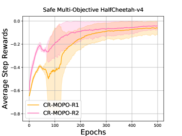
(a)

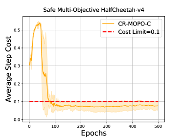
(b)

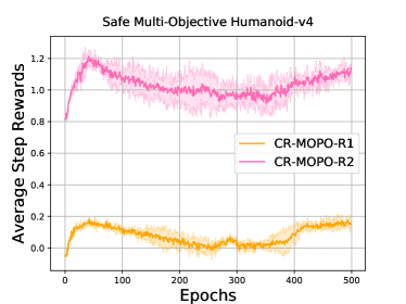
(c)

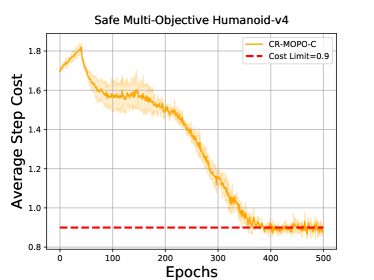
(d)

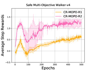
(e)

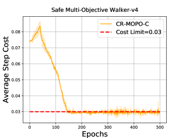
(f)

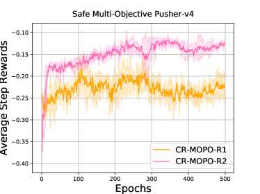
(g)

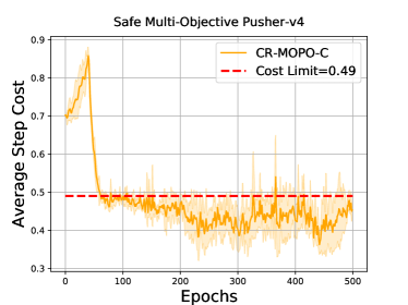
(h)

Figure 1: CR-MOPO on Safe Multi-Objective MuJoCo environments regarding the reward and safety performance.

Comparison experiments with CRPO [44] on Safe Multi-Objective HalfCheetah Environments. We develop a novel algorithm, the CR-MOPO-Soft (CR-MOPO-S) constraints’ algorithm, that can handle the safety constraint as one of the objectives. In CR-MOPO-S, we do not need to include the constraint in the objective. Instead, we incorporate the constraint in our method with a weight for performance (e.g., the weight can be 1.0). We hypothesize that by considering the constraint, we can navigate into a deep safe set, allowing us to concentrate on improving performance. This is especially relevant when the system is highly constrained, as operating near the boundary of the safe set can easily lead to constraint violations and "oscillations" behaviors from safe learning methods, e.g., CRPO [44], CPO [2], PCPO [46]. Intuitively, if we consistently operate at the safety boundary, we may encounter a conflict between safety and performance. Drawing an analogy to running on a road, if we position ourselves close to the edge, stepping out of the road would require effort to retreat, potentially compromising speed. However, suppose we realize the importance of running in the center of the road. In that case, we can prioritize safety and maximizing speed simultaneously. To hammer in the insight, we expand on the examples and scenarios we consider. We focus on a simple CMDP setup, prioritizing the maximization of rewards by incorporating safety violations as one of the objectives. We compare our algorithms, CR-MOPO and CR-MOPO-S, with a strong safe RL baseline, CRPO. In CRPO[44], the multiple tasks are scaled linearly into one objective. CRPO is a safe RL algorithm that can show better performance than safe RL algorithms, such as CPO [2], IPO [26], and unsafe RL algorithms such as TRPO [32] in terms of the balance between reward and safety violation. As shown in Figure 2, the experiment results demonstrate that our algorithms, CR-MOPO and CR-MOPO-S show better performance than CRPO regarding the reward and safety performance. And also, Our algorithms show a faster convergence rate than CRPO[44]. The detailed implementation is provided in Appendix B.2.

(a)

(b)

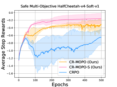
(c)

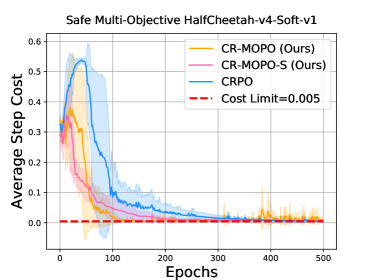
(d)

Figure 2: (a) and (b) show two of the Safe Multi-Objective MuJoCO environments, Safe Multi-Objective Humanoid and Pusher. (c) and (d) show the comparison results in terms of CR-MOPO, CR-MOPO-S and CRPO [44] on a Safe Multi-Objective MuJoCo environment, Safe Multi-Objective HalfCheetah, the cost limit is $0.005$, we start to optimize safety violation after $40$ Epochs.

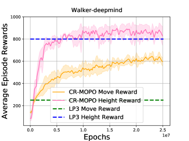
(a)

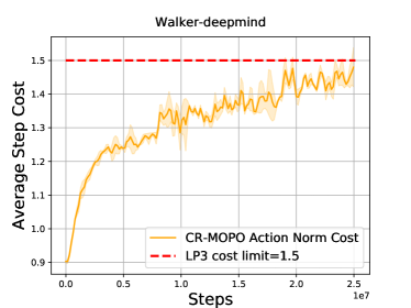
(b)

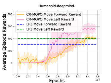
(c)

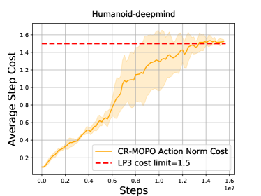
(d)

Figure 3: Compared with the DeepMind’s method, LP3 [17], on Safe Multi-Objective Walker-dm and Safe Multi-Objective Humanoid-dm environments.

Comparison experiments with LP3 [17] on Different Safe Multi-Objective Humanoid-dm and Walker-dm. LP3 [17] is a SOTA-safe multi-objective RL baseline proposed by DeepMind. They achieve safe multi-objective RL by leveraging the learning preferences, and they also deploy their methods on several challenging tasks, e.g., Humanoid-dm and Walker-dm that are from the DeepMind Control Suite [35]. In this section, we compare our algorithm with LP3 on the same environment settings. As shown in Figure 3, our algorithm can show remarkably better performance than LP3 [17] while guaranteeing safety. As shown in Figure 3 (a) and (b), in the Walker-dm task, when the cost limit is $1.5$, and our method can perform very well, e.g., the move reward is more than 800, and the height reward is more than 600; in the same setting, using LP3 [17], the move reward can only be more than 250, and the height reward is about 800. For Humanoid-dm, LP3 can achieve about 400 and 300 regarding the move left and move forward reward when the cost limit is 1.5. However, our method can achieve at least 400 regarding the move left reward and about 600 regarding the move forward reward. The experiment results demonstrate that our method performs significantly better than LP3 [17].

One explanation of the better results compared to LP3, could be that our methods can optimize policies to the boundaries of the constraint thresholds. Although this results in not conservative policies, this can easily be remedied by choosing more conservative constraint thresholds.

7 Conclusion

In this study, we try to balance each task’s performance in a multi-task RL setting. Further, we achieve each task rewards monotonic improvement and ensure policy safety. A primal-based safe multi-task RL framework is proposed, where multiple objectives between different tasks are optimized by analyzing the conflict gradient manipulation, and the constraint rectification is leveraged to search for the safety policy during multiple objectives’ exploration. Moreover, the convergence and safety violation analysis are provided. Finally, we deploy our practical algorithms on several challenging, safe multi-task RL environments and compare our method with the SOTA safe RL baseline and safe multi-task RL algorithms. The experiment results indicate that our method can perform better than SOTA-safe RL baselines and SOTA-safe multi-task RL algorithms regarding the balance between each task performance and safety violation. It is necessary to address how to deploy our algorithm in real-world scenarios and try to leverage the foundation models [45] with our method to address safe multi-task RL robustness problems. A conceivable adverse societal consequence arises from the potential misapplication of this work within safety-critical contexts, which could lead to unforeseen damages. It is our aspiration that our discoveries catalyze further investigations into the safety and generalizability of reinforcement learning in secure environments.

Appendix

Appendix A Proof

We prove the results of Theorem 5.2 in two parts. We give the TD-Learning results in Theorem A.6 in section A.1, and the unbiased q-estimation estimator results in Theorem A.10 in section A.2.

Lemma A.1 (Multi-objective NPG)

Given the preference vector $\boldsymbol{\lambda}$ and considering the multi-objective NPG update $w_{t+1}=w_{t}-\eta\tilde{F}(w_{t})^{\dagger}\sum_{i=1}^{m}\lambda^{i}\nabla f_{i}\left(\pi_{w_{t}}\right)$, where $\tilde{F}(w)=\mathbb{E}_{\nu_{\pi_{w}}}\left[\phi_{w}(s,a)\phi_{w}(s,a)^{\top}\right]$ in the tabular setting, the multi-objective NPG update also takes the form:

$$w_{t+1}=w_{t}+\frac{\eta}{1-\gamma}\sum_{i=1}^{m}\lambda^{i}Q_{i}^{\pi_{w_{t}}},\quad\quad\pi_{w_{t+1}}(a\mid s)=\pi_{w_{t}}(a\mid s)\frac{\exp\left(\eta\sum_{i=1}^{m}\lambda_{i}Q_{i}^{\pi_{w_{t}}}/(1-\gamma)\right)}{Z_{t}(s)}.$$

where

$$Z_{t}(s)=\sum_{a\in\mathcal{A}}\pi_{w_{t}}(a\mid s)\exp{\left(\frac{\eta\sum_{i=1}^{m}\lambda_{i}{Q}_{i}^{\pi_{w_{t}}}(s,a)}{1-\gamma}\right)}$$

Proof. From Lemma 5.1 in [3], we know

$$\tilde{F}(w_{t})^{\dagger}\nabla f_{i}\left(\pi_{w_{t}}\right)=\frac{A_{i}^{\pi_{w_{t}}}}{1-\gamma}+v$$

where $v\in\mathbb{R}^{|\mathcal{S}||\mathcal{A}|}$ and $v_{s,a}=c_{s}\text{ for some }c_{s}\in\mathbb{R}\text{ for each state }s$ and action $a$. This yields the updates

$$w_{t+1}=w_{t}+\frac{\eta}{1-\gamma}\sum_{i=1}^{m}\lambda^{i}A_{i}^{\pi_{w_{t}}}+\eta v\sum_{i=1}^{m}\lambda^{i}\quad$$

and

$$\pi_{w_{t+1}}(a\mid s)=\pi_{w_{t}}(a\mid s)\frac{\exp\left(\eta\sum_{i=1}^{m}\lambda_{i}A_{i}^{\pi_{w_{t}}}/(1-\gamma)+\eta c_{s}\sum_{i=1}^{m}\lambda_{i}\right)}{Z_{t}(s)}.$$

Owing to the normalization factor $Z_{t}(s)$, the state-dependent offset $c_{s}$ cancels in the updates for $\pi$, so that resulting policy is invariant to the specific choice of $c_{s}$. Hence, we pick $c_{s}\equiv 0$, which yields the updates

$$w_{t+1}=w_{t}+\frac{\eta}{1-\gamma}\sum_{i=1}^{m}\lambda^{i}A_{i}^{\pi_{w_{t}}}$$

and

$$\pi_{w_{t+1}}(a\mid s)=\pi_{w_{t}}(a\mid s)\frac{\exp\left(\eta\sum_{i=1}^{m}\lambda^{i}A_{i}^{\pi_{w_{t}}}/(1-\gamma)\right)}{Z_{t}(s)}$$

Finally, the advantage function $A_{i}^{\pi_{w}}(s,a)=Q_{i}^{\pi_{w}}(s,a)-V_{i}^{\pi_{w}}(s,a)$ can be replaced by the Q-function $Q_{i}^{\pi_{w}}(s,a)$ due to the normalization factor $Z_{t}(s)$, which yields the the statement of the lemma.

$\Box$

Lemma A.2

Performance improvement bound for approximated multi-objective NPG. For the iterates $\pi_{w_{t}}$ generated by the approximated multi-objective NPG updates in the tabular setting, we have the following holds

$$\sum_{i=1}^{m}\lambda^{i}\left(f_{i}\left(w_{t+1}\right)-f_{i}\left(w_{t}\right)\right)$$

$${\geq} \frac{1-\gamma}{\eta}\mathbb{E}_{s\sim\rho}\left(\log Z_{t}(s)-\frac{\eta}{1-\gamma}\sum_{i=1}^{m}\lambda^{i}V^{\pi_{w_{t}}}_{i}(s)+\frac{\eta}{1-\gamma}\sum_{a\in\mathcal{A}}\pi_{w_{t}}(a\mid s)\sum_{i=1}^{m}\lambda^{i}\left(Q^{\pi_{w_{t}}}_{i}(s,a)-\bar{Q}^{t}_{i}(s,a)\right)\right)$$

$$-\frac{1}{1-\gamma}\mathbb{E}_{s\sim\nu_{\rho}}\sum_{a\in\mathcal{A}}\pi_{w_{t}}(a\mid s)\sum_{i=1}^{m}\lambda^{i}\left(Q^{\pi_{w_{t}}}_{i}(s,a)-\bar{Q}^{t}_{i}(s,a)\right)$$

$$+\frac{1}{1-\gamma}\mathbb{E}_{s\sim\nu_{\rho}}\sum_{a\in\mathcal{A}}\pi_{w_{t+1}}(a\mid s)\sum_{i=1}^{m}\lambda^{i}\left(Q^{\pi_{w_{t}}}_{i}(s,a)-\bar{Q}^{t}_{i}(s,a)\right).$$

Proof. We first provide the following lower bound.

$$\log Z_{t}(s)-\frac{\eta}{1-\gamma}\sum_{i=1}^{m}\lambda^{i}V^{\pi_{w_{t}}}_{i}(s)$$

$$=\log\sum_{a\in\mathcal{A}}\pi_{w_{t}}(a\mid s)\exp\left(\frac{\eta\sum_{i=1}^{m}\lambda^{i}\bar{Q}^{t}_{i}(s,a)}{1-\gamma}\right)-\frac{\eta}{1-\gamma}\sum_{i=1}^{m}\lambda^{i}V^{\pi_{w_{t}}}_{i}(s)$$

$$\geq\sum_{a\in\mathcal{A}}\pi_{w_{t}}(a\mid s)\log\exp\left(\frac{\eta\sum_{i=1}^{m}\lambda^{i}\bar{Q}^{t}_{i}(s,a)}{1-\gamma}\right)-\frac{\eta}{1-\gamma}\sum_{i=1}^{m}\lambda^{i}V^{\pi_{w_{t}}}_{i}(s)$$

$$=\frac{\eta}{1-\gamma}\sum_{a\in\mathcal{A}}\pi_{w_{t}}(a\mid s)\sum_{i=1}^{m}\lambda^{i}\left(\bar{Q}^{t}_{i}(s,a)-Q^{\pi_{w_{t}}}_{i}(s,a)\right)$$

$$+\frac{\eta}{1-\gamma}\sum_{a\in\mathcal{A}}\pi_{w_{t}}(a\mid s)\sum_{i=1}^{m}\lambda^{i}Q^{\pi_{w_{t}}}_{i}(s,a)-\frac{\eta}{1-\gamma}\sum_{i=1}^{m}\lambda^{i}V^{\pi_{w_{t}}}_{i}(s)$$

$$=\frac{\eta}{1-\gamma}\sum_{a\in\mathcal{A}}\pi_{w_{t}}(a\mid s)\sum_{i=1}^{m}\lambda^{i}\left(\bar{Q}^{t}_{i}(s,a)-Q^{\pi_{w_{t}}}_{i}(s,a)\right)$$

Thus, we conclude that

$$\log Z_{t}(s)-\frac{\eta}{1-\gamma}\sum_{i=1}^{m}\lambda^{i}V^{\pi_{w_{t}}}_{i}(s)+\frac{\eta}{1-\gamma}\sum_{a\in\mathcal{A}}\pi_{w_{t}}(a\mid s)\sum_{i=1}^{m}\lambda^{i}\left(Q^{\pi_{w_{t}}}_{i}(s,a)-\bar{Q}^{t}_{i}(s,a)\right)\geq 0.$$ (10)

We then proceed to prove this lemma. The performance difference lemma [19] implies:

$$\sum_{i=1}^{m}\lambda^{i}\left(f_{i}\left(w_{t+1}\right)-f_{i}\left(w_{t}\right)\right)$$

$$=\frac{1}{1-\gamma}\mathbb{E}_{s\sim\nu_{\rho}}\sum_{a\in\mathcal{A}}\pi_{w_{t+1}}(a\mid s)\sum_{i=1}^{m}\lambda^{i}A^{\pi_{w_{t}}}_{i}(s,a)$$

$$=\frac{1}{1-\gamma}\mathbb{E}_{s\sim\nu_{\rho}}\sum_{a\in\mathcal{A}}\pi_{w_{t+1}}(a\mid s)\sum_{i=1}^{m}\lambda^{i}Q^{\pi_{w_{t}}}_{i}(s,a)-\frac{1}{1-\gamma}\mathbb{E}_{s\sim\nu_{\rho}}\sum_{i=1}^{m}\lambda^{i}V^{\pi_{w_{t}}}_{i}(s)$$

$$=\frac{1}{1-\gamma}\mathbb{E}_{s\sim\nu_{\rho}}\sum_{a\in\mathcal{A}}\pi_{w_{t+1}}(a\mid s)\sum_{i=1}^{m}\lambda^{i}\bar{Q}^{t}_{i}(s,a)$$

$$+\frac{1}{1-\gamma}\mathbb{E}_{s\sim\nu_{\rho}}\sum_{a\in\mathcal{A}}\pi_{w_{t+1}}(a\mid s)\sum_{i=1}^{m}\lambda^{i}\left(Q^{\pi_{w_{t}}}_{i}(s,a)-\bar{Q}^{t}_{i}(s,a)\right)-\frac{1}{1-\gamma}\mathbb{E}_{s\sim\nu_{\rho}}\sum_{i=1}^{m}\lambda^{i}V^{\pi_{w_{t}}}_{i}(s)$$

$$\stackrel{{\scriptstyle(i)}}{{=}}\frac{1}{\eta}\mathbb{E}_{s\sim\nu_{\rho}}\sum_{a\in\mathcal{A}}\pi_{w_{t+1}}(a\mid s)\log\left(\frac{\pi_{w_{t+1}}(a\mid s)Z_{t}(s)}{\pi_{w_{t}}(a\mid s)}\right)$$

$$+\frac{1}{1-\gamma}\mathbb{E}_{s\sim\nu_{\rho}}\sum_{a\in\mathcal{A}}\pi_{w_{t+1}}(a\mid s)\sum_{i=1}^{m}\lambda^{i}\left(Q^{\pi_{w_{t}}}_{i}(s,a)-\bar{Q}^{t}_{i}(s,a)\right)-\frac{1}{1-\gamma}\mathbb{E}_{s\sim\nu_{\rho}}\sum_{i=1}^{m}\lambda^{i}V^{\pi_{w_{t}}}_{i}(s)$$

$$=\frac{1}{\eta}\mathbb{E}_{s\sim\nu_{\rho}}D_{\mathrm{KL}}\left(\pi_{w_{t+1}}||\pi_{w_{t}}\right)+\frac{1}{\eta}\mathbb{E}_{s\sim\nu_{\rho}}\log Z_{t}(s)$$

$$+\frac{1}{1-\gamma}\mathbb{E}_{s\sim\nu_{\rho}}\sum_{a\in\mathcal{A}}\pi_{w_{t+1}}(a\mid s)\sum_{i=1}^{m}\lambda^{i}\left(Q^{\pi_{w_{t}}}_{i}(s,a)-\bar{Q}^{t}_{i}(s,a)\right)-\frac{1}{1-\gamma}\mathbb{E}_{s\sim\nu_{\rho}}\sum_{i=1}^{m}\lambda^{i}V^{\pi_{w_{t}}}_{i}(s)$$

$$\geq\frac{1}{\eta}\mathbb{E}_{s\sim\nu_{\rho}}\left(\log Z_{t}(s)-\frac{\eta}{1-\gamma}\sum_{i=1}^{m}\lambda^{i}V^{\pi_{w_{t}}}_{i}(s)+\frac{\eta}{1-\gamma}\sum_{a\in\mathcal{A}}\pi_{w_{t}}(a\mid s)\sum_{i=1}^{m}\lambda^{i}\left(Q^{\pi_{w_{t}}}_{i}(s,a)-\bar{Q}^{t}_{i}(s,a)\right)\right)$$

$$-\frac{1}{1-\gamma}\mathbb{E}_{s\sim\nu_{\rho}}\sum_{a\in\mathcal{A}}\pi_{w_{t}}(a\mid s)\sum_{i=1}^{m}\lambda^{i}\left(Q^{\pi_{w_{t}}}_{i}(s,a)-\bar{Q}^{t}_{i}(s,a)\right)$$

$$+\frac{1}{1-\gamma}\mathbb{E}_{s\sim\nu_{\rho}}\sum_{a\in\mathcal{A}}\pi_{w_{t+1}}(a\mid s)\sum_{i=1}^{m}\lambda^{i}\left(Q^{\pi_{w_{t}}}_{i}(s,a)-\bar{Q}^{t}_{i}(s,a)\right)$$

$$\stackrel{{\scriptstyle(ii)}}{{\geq}}\frac{1-\gamma}{\eta}\mathbb{E}_{s\sim\rho}\left(\log Z_{t}(s)-\frac{\eta}{1-\gamma}\sum_{i=1}^{m}\lambda^{i}V^{\pi_{w_{t}}}_{i}(s)+\frac{\eta}{1-\gamma}\sum_{a\in\mathcal{A}}\pi_{w_{t}}(a\mid s)\sum_{i=1}^{m}\lambda^{i}\left(Q^{\pi_{w_{t}}}_{i}(s,a)-\bar{Q}^{t}_{i}(s,a)\right)\right)$$

$$-\frac{1}{1-\gamma}\mathbb{E}_{s\sim\nu_{\rho}}\sum_{a\in\mathcal{A}}\pi_{w_{t}}(a\mid s)\sum_{i=1}^{m}\lambda^{i}\left(Q^{\pi_{w_{t}}}_{i}(s,a)-\bar{Q}^{t}_{i}(s,a)\right)$$

$$+\frac{1}{1-\gamma}\mathbb{E}_{s\sim\nu_{\rho}}\sum_{a\in\mathcal{A}}\pi_{w_{t+1}}(a\mid s)\sum_{i=1}^{m}\lambda^{i}\left(Q^{\pi_{w_{t}}}_{i}(s,a)-\bar{Q}^{t}_{i}(s,a)\right)$$

where $(i)$ follows from the update rule in Lemma A.1 and $(ii)$ follows from the facts that $\left\lVert\nu_{\rho}/\rho\right\rVert\geq 1-\gamma$ and (10). $\Box$

Lemma A.3

Expected optimality gap for approximated multi-objective NPG. Consider the approximated NPG updates in the tabular setting. We have

$$\sum_{i=1}^{m}\lambda^{i}\left(f_{i}\left(\pi^{*}\right)-f_{i}\left(\pi_{w_{t}}\right)\right)$$

$${\leq}\frac{1}{\eta}\mathbb{E}_{s\sim\nu^{*}}\left(D_{\mathrm{KL}}\left(\pi^{*}\|\pi_{w_{t}}\right)-D_{\mathrm{KL}}\left(\pi^{*}\|\pi_{w_{t+1}}\right)\right)+\frac{2\eta r_{\max}}{(1-\gamma)^{2}}\sum_{i=1}^{m}\lambda^{i}\left\|\sum_{i=1}^{m}\lambda^{i}\bar{Q}_{t}^{i}\right\|_{2}$$

$$+\frac{1}{(1-\gamma)^{2}}\mathbb{E}_{s\sim\nu_{\rho}}\sum_{a\in\mathcal{A}}\pi_{w_{t}}(a\mid s)\sum_{i=1}^{m}\lambda^{i}\left(Q^{\pi_{w_{t}}}_{i}(s,a)-\bar{Q}^{t}_{i}(s,a)\right)$$

$$-\frac{1}{(1-\gamma)^{2}}\mathbb{E}_{s\sim\nu_{\rho}}\sum_{a\in\mathcal{A}}\pi_{w_{t+1}}(a\mid s)\sum_{i=1}^{m}\lambda^{i}\left(Q^{\pi_{w_{t}}}_{i}(s,a)-\bar{Q}^{t}_{i}(s,a)\right)$$

$$+\frac{1}{1-\gamma}\mathbb{E}_{s\sim\nu^{*}}\sum_{a\in\mathcal{A}}\pi^{*}(a\mid s)\sum_{i=1}^{m}\lambda^{i}\left(Q^{\pi^{w_{t}}}_{i}(s,a)-\bar{Q}^{t}_{i}(s,a)\right)$$

Proof.

$$\sum_{i=1}^{m}\lambda^{i}\left(f_{i}\left(\pi^{*}\right)-f_{i}\left(\pi_{w_{t}}\right)\right)$$

$$=\frac{1}{1-\gamma}\mathbb{E}_{s\sim\nu^{*}}\sum_{a\in\mathcal{A}}\pi^{*}(a\mid s)\sum_{i=1}^{m}\lambda^{i}A^{\pi_{w_{t}}}_{i}(s,a)$$

$$=\frac{1}{1-\gamma}\mathbb{E}_{s\sim\nu^{*}}\sum_{a\in\mathcal{A}}\pi^{*}(a\mid s)\sum_{i=1}^{m}\lambda^{i}Q^{\pi_{w_{t}}}_{i}(s,a)-\frac{1}{1-\gamma}\mathbb{E}_{s\sim\nu^{*}}\sum_{i=1}^{m}\lambda^{i}V^{\pi_{w_{t}}}_{i}(s)$$

$$=\frac{1}{1-\gamma}\mathbb{E}_{s\sim\nu^{*}}\sum_{a\in\mathcal{A}}\pi^{*}(a\mid s)\sum_{i=1}^{m}\lambda^{i}\bar{Q}^{t}_{i}(s,a)+\frac{1}{1-\gamma}\mathbb{E}_{s\sim\nu^{*}}\sum_{a\in\mathcal{A}}\pi^{*}(a\mid s)\sum_{i=1}^{m}\lambda^{i}\left(Q^{\pi_{w_{t}}}_{i}(s,a)-\bar{Q}^{t}_{i}(s,a)\right)$$

$$-\frac{1}{1-\gamma}\mathbb{E}_{s\sim\nu^{*}}\sum_{i=1}^{m}\lambda^{i}V^{\pi_{w_{t}}}_{i}(s)$$

$$\stackrel{{\scriptstyle(i)}}{{=}}\frac{1}{\eta}\mathbb{E}_{s\sim\nu^{*}}\sum_{a\in\mathcal{A}}\pi^{*}(a\mid s)\log\frac{\pi_{w_{t+1}}(a\mid s)Z_{t}(s)}{\pi_{w_{t}}(a\mid s)}+\frac{1}{1-\gamma}\mathbb{E}_{s\sim\nu^{*}}\sum_{a\in\mathcal{A}}\pi^{*}(a\mid s)\sum_{i=1}^{m}\lambda^{i}\left(Q^{\pi_{w_{t}}}_{i}(s,a)-\bar{Q}^{t}_{i}(s,a)\right)$$

$$-\frac{1}{1-\gamma}\mathbb{E}_{s\sim\nu^{*}}\sum_{i=1}^{m}\lambda^{i}V^{\pi_{w_{t}}}_{i}(s)$$

$$=\frac{1}{\eta}\mathbb{E}_{s\sim\nu^{*}}\left(D_{\mathrm{KL}}\left(\pi^{*}||\pi_{w_{t}}\right)-D_{\mathrm{KL}}\left(\pi^{*}||\pi_{w_{t+1}}\right)\right)+\frac{1}{1-\gamma}\mathbb{E}_{s\sim\nu^{*}}\sum_{a\in\mathcal{A}}\pi^{*}(a\mid s)\sum_{i=1}^{m}\lambda^{i}\left(Q^{\pi_{w_{t}}}_{i}(s,a)-\bar{Q}^{t}_{i}(s,a)\right)$$

$$+\frac{1}{\eta}\mathbb{E}_{s\sim\nu^{*}}\left(\log Z_{t}(s)-\frac{\eta}{1-\gamma}\sum_{i=1}^{m}\lambda^{i}V^{\pi_{w_{t}}}_{i}(s)\right)$$

$$\leq\frac{1}{\eta}\mathbb{E}_{s\sim\nu^{*}}\left(D_{\mathrm{KL}}\left(\pi^{*}||\pi_{w_{t}}\right)-D_{\mathrm{KL}}\left(\pi^{*}||\pi_{w_{t+1}}\right)\right)$$

$$+\frac{1}{\eta}\mathbb{E}_{s\sim\nu^{*}}\left(\log Z_{t}(s)-\frac{\eta}{1-\gamma}\sum_{i=1}^{m}\lambda^{i}V^{\pi_{w_{t}}}_{i}(s)+\frac{\eta}{1-\gamma}\sum_{a\in\mathcal{A}}\pi_{w_{t}}(a\mid s)\sum_{i=1}^{m}\lambda^{i}\left(Q^{\pi_{w_{t}}}_{i}(s,a)-\bar{Q}^{t}_{i}(s,a)\right)\right)$$

$$+\frac{1}{1-\gamma}\mathbb{E}_{s\sim\nu^{*}}\sum_{a\in\mathcal{A}}\pi^{*}(a\mid s)\sum_{i=1}^{m}\lambda^{i}\left(Q^{\pi_{w_{t}}}_{i}(s,a)-\bar{Q}^{t}_{i}(s,a)\right)$$

$$\stackrel{{\scriptstyle(ii)}}{{\leq}}\frac{1}{\eta}\mathbb{E}_{s\sim\nu^{*}}\left(D_{\mathrm{KL}}\left(\pi^{*}\|\pi_{w_{t}}\right)-D_{\mathrm{KL}}\left(\pi^{*}\|\pi_{w_{t+1}}\right)\right)+\frac{1}{1-\gamma}\sum_{i=1}^{m}\lambda^{i}\left(f_{i}^{\nu^{*}}\left(w_{t+1}\right)-f_{i}^{\nu^{*}}\left(w_{t}\right)\right)$$

$$+\frac{1}{(1-\gamma)^{2}}\mathbb{E}_{s\sim\nu_{\rho}}\sum_{a\in\mathcal{A}}\pi_{w_{t}}(a\mid s)\sum_{i=1}^{m}\lambda^{i}\left(Q^{\pi_{w_{t}}}_{i}(s,a)-\bar{Q}^{t}_{i}(s,a)\right)$$

$$-\frac{1}{(1-\gamma)^{2}}\mathbb{E}_{s\sim\nu_{\rho}}\sum_{a\in\mathcal{A}}\pi_{w_{t+1}}(a\mid s)\sum_{i=1}^{m}\lambda^{i}\left(Q^{\pi_{w_{t}}}_{i}(s,a)-\bar{Q}^{t}_{i}(s,a)\right)$$

$$+\frac{1}{1-\gamma}\mathbb{E}_{s\sim\nu^{*}}\sum_{a\in\mathcal{A}}\pi^{*}(a\mid s)\sum_{i=1}^{m}\lambda^{i}\left(Q^{\pi^{w_{t}}}_{i}(s,a)-\bar{Q}^{t}_{i}(s,a)\right)$$

$$\stackrel{{\scriptstyle(iii)}}{{\leq}}\frac{1}{\eta}\mathbb{E}_{s\sim\nu^{*}}\left(D_{\mathrm{KL}}\left(\pi^{*}\|\pi_{w_{t}}\right)-D_{\mathrm{KL}}\left(\pi^{*}\|\pi_{w_{t+1}}\right)\right)+\frac{2r_{\max}}{(1-\gamma)^{2}}\sum_{i=1}^{m}\lambda^{i}\left\|w_{t+1}-w_{t}\right\|_{2}$$

$$+\frac{1}{(1-\gamma)^{2}}\mathbb{E}_{s\sim\nu_{\rho}}\sum_{a\in\mathcal{A}}\pi_{w_{t}}(a\mid s)\sum_{i=1}^{m}\lambda^{i}\left(Q^{\pi_{w_{t}}}_{i}(s,a)-\bar{Q}^{t}_{i}(s,a)\right)$$

$$-\frac{1}{(1-\gamma)^{2}}\mathbb{E}_{s\sim\nu_{\rho}}\sum_{a\in\mathcal{A}}\pi_{w_{t+1}}(a\mid s)\sum_{i=1}^{m}\lambda^{i}\left(Q^{\pi_{w_{t}}}_{i}(s,a)-\bar{Q}^{t}_{i}(s,a)\right)$$

$$+\frac{1}{1-\gamma}\mathbb{E}_{s\sim\nu^{*}}\sum_{a\in\mathcal{A}}\pi^{*}(a\mid s)\sum_{i=1}^{m}\lambda^{i}\left(Q^{\pi^{w_{t}}}_{i}(s,a)-\bar{Q}^{t}_{i}(s,a)\right)$$

$$\stackrel{{\scriptstyle(iiii)}}{{\leq}}\frac{1}{\eta}\mathbb{E}_{s\sim\nu^{*}}\left(D_{\mathrm{KL}}\left(\pi^{*}\|\pi_{w_{t}}\right)-D_{\mathrm{KL}}\left(\pi^{*}\|\pi_{w_{t+1}}\right)\right)+\frac{2\eta r_{\max}}{(1-\gamma)^{2}}\sum_{i=1}^{m}\lambda^{i}\left\|\sum_{i=1}^{m}\lambda^{i}\bar{Q}_{t}^{i}\right\|_{2}$$

$$+\frac{1}{(1-\gamma)^{2}}\mathbb{E}_{s\sim\nu_{\rho}}\sum_{a\in\mathcal{A}}\pi_{w_{t}}(a\mid s)\sum_{i=1}^{m}\lambda^{i}\left(Q^{\pi_{w_{t}}}_{i}(s,a)-\bar{Q}^{t}_{i}(s,a)\right)$$

$$-\frac{1}{(1-\gamma)^{2}}\mathbb{E}_{s\sim\nu_{\rho}}\sum_{a\in\mathcal{A}}\pi_{w_{t+1}}(a\mid s)\sum_{i=1}^{m}\lambda^{i}\left(Q^{\pi_{w_{t}}}_{i}(s,a)-\bar{Q}^{t}_{i}(s,a)\right)$$

$$+\frac{1}{1-\gamma}\mathbb{E}_{s\sim\nu^{*}}\sum_{a\in\mathcal{A}}\pi^{*}(a\mid s)\sum_{i=1}^{m}\lambda^{i}\left(Q^{\pi^{w_{t}}}_{i}(s,a)-\bar{Q}^{t}_{i}(s,a)\right)$$

where $(i)$ and $(iiii)$ follow from Lemma A.1, $(ii)$ follows from Lemma A.2, and $(iii)$ follows from the Lipschitz property of $f_{i}^{\nu^{*}}\left(w\right)$ such that $f_{i}^{\nu^{*}}\left(w_{t+1}\right)-f_{i}^{\nu^{*}}\left(w_{t}\right)\leq\frac{2c_{\text{max}}}{1-\gamma}\left\lVert w_{t+1}-w_{t}\right\rVert_{2}$. $\Box$

A.1 TD-Learning

Lemma A.4 ([10])

Consider the iteration given in (3) with arbitrary initialization $Q_{0}^{i}$. Assume that the stationary distribution $\mu_{\pi_{w}}$ is not degenerate for all $w\in\mathbb{R}^{|\mathcal{S}|\times|\mathcal{A}|}$. Let stepsize $\ell_{k}=\Theta\left(\frac{1}{k^{\sigma}}\right)(0<\sigma<1)$. Then, with probability at least $1-\delta$, we have

$$\left\|Q_{K}^{i}-Q_{\pi_{w}}^{i}\right\|_{2}=\mathcal{O}\left(\frac{\log\left(|\mathcal{S}|^{2}|\mathcal{A}|^{2}K^{2}/\delta\right)}{(1-\gamma)K^{\sigma/2}}\right).$$

Note that $\sigma$ can be arbitrarily close to 1 . Lemma 2 implies that we can obtain an approximation $\bar{Q}_{t}^{i}$ such that $\left\|\bar{Q}_{t}^{i}-Q_{\pi_{w}}^{i}\right\|_{2}=\widetilde{\mathcal{O}}\left(1/\sqrt{K_{\text{TD}}}\right)$ with high probability.

Lemma A.5

If

$$\beta> \frac{2}{\eta T}\mathbb{E}_{s\sim\nu^{*}}D_{\mathrm{KL}}\left(\pi^{*}||\pi_{w_{0}}\right)+\frac{4\eta r_{\max}^{2}|\mathcal{S}||\mathcal{A}|}{(1-\gamma)^{4}T}\left(\left[\sum_{t\in\mathcal{N}_{0}}\left(\sum_{i=1}^{m}\lambda^{i}_{t}\right)^{2}\right]+T-\left|\mathcal{N}_{0}\right|\right)$$ (11)

$$+\frac{6}{(1-\gamma)^{2}T}\left(\sum_{t\in\mathcal{N}_{0}}\sum_{i=1}^{m}\lambda_{t}^{i}\left\|Q_{\pi_{w_{t}}}^{i}-\bar{Q}_{t}^{i}\right\|_{2}+\sum_{i=m+1}^{m+p}\sum_{t\in\mathcal{N}_{i}}\left\|Q_{\pi_{w_{t}}^{i}}^{i}-\bar{Q}_{t}^{i}\right\|_{2}\right),$$

then we have the following holds:

1. $\mathcal{N}_{0}\neq\emptyset$,

2. One of the following two statements must hold,

   1. $\left|\mathcal{N}_{0}\right|\geq\frac{T}{2}$,

   2. $\sum_{t\in\mathcal{N}_{0}}\sum_{i=1}^{m}\lambda_{t}^{i}\left(f_{i}\left(\pi^{*}\right)-f_{i}\left(\pi_{w_{t}}\right)\right)\leq 0$.

Proof. When $t\in\mathcal{N}_{0}$, from Lemma A.3 we have

$$\sum_{i=1}^{m}\lambda^{i}\left(f_{i}\left(\pi^{*}\right)-f_{i}\left(\pi_{w_{t}}\right)\right) \leq\frac{1}{\eta}\mathbb{E}_{s\sim\nu^{*}}\left(D_{\mathrm{KL}}\left(\pi^{*}||\pi_{w_{t}}\right)-D_{\mathrm{KL}}\left(\pi^{*}||\pi_{w_{t+1}}\right)\right)+\frac{2\eta c_{\max}^{2}|\mathcal{S}||\mathcal{A}|}{(1-\gamma)^{4}}(\sum_{i=1}^{m}\lambda^{i})^{2}$$

$$+\frac{3}{(1-\gamma)^{2}}\sum_{i=1}^{m}\lambda^{i}\left\|Q_{\pi_{w_{t}}}^{i}-\bar{Q}_{t}^{i}\right\|_{2}.$$ (12)

Similarly, when $t\in\mathcal{N}_{i}(i\neq 0)$ we have

$$f_{i}\left(\pi_{w_{t}}\right)-f_{i}\left(\pi^{*}\right) \leq\frac{1}{\eta}\mathbb{E}_{s\sim\nu^{*}}\left(D_{\mathrm{KL}}\left(\pi^{*}||\pi_{w_{t}}\right)-D_{\mathrm{KL}}\left(\pi^{*}||\pi_{w_{t+1}}\right)\right)+\frac{2\eta c_{\max}^{2}|\mathcal{S}||\mathcal{A}|}{(1-\gamma)^{4}}$$

$$+\frac{3}{(1-\gamma)^{2}}\left\|Q_{\pi_{w_{t}}}^{i}-\bar{Q}_{t}^{i}\right\|_{2}.$$ (13)

Taking the summation of (A.1) and (A.1) from $t=0$ to $T-1$ gives

$$\sum_{t\in\mathcal{N}_{0}}\sum_{i=1}^{m}\lambda_{t}^{i}\left(f_{i}\left(\pi^{*}\right)-f_{i}\left(\pi_{w_{t}}\right)\right)+\sum_{i=1}^{p}\sum_{t\in\mathcal{N}_{i}}\left(f_{i}\left(\pi_{w_{t}}\right)-f_{i}\left(\pi^{*}\right)\right)$$ (14)

$$\leq\frac{1}{\eta}\mathbb{E}_{s\sim\nu^{*}}D_{\mathrm{KL}}\left(\pi^{*}||\pi_{w_{0}}\right)+\frac{2\eta c_{\max}^{2}|\mathcal{S}||\mathcal{A}|}{(1-\gamma)^{4}}\left(\sum_{t\in\mathcal{N}_{0}}\left(\sum_{i=1}^{m}\lambda^{i}_{t}\right)^{2}+T-\left|\mathcal{N}_{0}\right|\right)$$

$$+\frac{3}{(1-\gamma)^{2}}\left(\sum_{t\in\mathcal{N}_{0}}\sum_{i=1}^{m}\lambda^{i}\left\|Q_{\pi_{w_{t}}}^{i}-\bar{Q}_{t}^{i}\right\|_{2}+\sum_{i=m+1}^{m+p}\sum_{t\in\mathcal{N}_{i}}\left\|Q_{\pi_{w_{t}}^{i}}^{i}-\bar{Q}_{t}^{i}\right\|_{2}\right).$$

Note that when $t\in\mathcal{N}_{i}(i\neq 0)$, we have $\bar{f}_{i}\left(w_{t}\right)>c_{i}+\beta$ (line 9 in Algorithm 1), which implies that

$$f_{i}\left(\pi_{w_{t}}\right)-f_{i}\left(\pi^{*}\right) \geq\bar{f}_{i}\left(w_{t}^{i}\right)-f_{i}\left(\pi^{*}\right)-\left|\bar{f}_{i}\left(w_{t}^{i}\right)-f_{i}\left(\pi_{w_{t}}\right)\right|$$

$$\geq c_{i}+\beta-J_{i}\left(\pi^{*}\right)-\left|\bar{f}_{i}\left(w_{t}^{i}\right)-f_{i}\left(\pi_{w_{t}}\right)\right|$$

$$\geq\beta-\left\|Q_{\pi_{w}}^{i}-\bar{Q}_{t}^{i}\right\|_{2}.$$ (15)

Substituting (A.1) into (14) gives

$$\sum_{t\in\mathcal{N}_{0}}\sum_{i=1}^{m}\lambda_{t}^{i}\left(f_{i}\left(\pi^{*}\right)-f_{i}\left(\pi_{w_{t}}\right)\right)+\beta\sum_{i=1}^{p}\left|\mathcal{N}_{i}\right|-\sum_{i=m+1}^{m+p}\sum_{t\in\mathcal{N}_{i}}\left\|Q_{\pi_{w}}^{i}-\bar{Q}_{t}^{i}\right\|_{2}$$

$$\leq \frac{1}{\eta}\mathbb{E}_{s\sim\nu^{*}}D_{\mathrm{KL}}\left(\pi^{*}||\pi_{w_{0}}\right)+\frac{2\eta c_{\max}^{2}|\mathcal{S}||\mathcal{A}|}{(1-\gamma)^{4}}\left(\sum_{t\in\mathcal{N}_{0}}\left(\sum_{i=1}^{m}\lambda^{i}_{t}\right)^{2}+T-\left|\mathcal{N}_{0}\right|\right)$$

$$+\frac{3}{(1-\gamma)^{2}}\left(\sum_{t\in\mathcal{N}_{0}}\sum_{i=1}^{m}\lambda^{i}\left\|Q_{\pi_{w_{t}}}^{i}-\bar{Q}_{t}^{i}\right\|_{2}+\sum_{i=m+1}^{m+p}\sum_{t\in\mathcal{N}_{i}}\left\|Q_{\pi_{w_{t}}^{i}}^{i}-\bar{Q}_{t}^{i}\right\|_{2}\right),$$

which implies

$$\sum_{t\in\mathcal{N}_{0}}\sum_{i=1}^{m}\lambda_{t}^{i}\left(f_{i}\left(\pi^{*}\right)-f_{i}\left(\pi_{w_{t}}\right)\right)+\beta\sum_{i=1}^{p}\left|\mathcal{N}_{i}\right|$$ (16)

$$\leq \frac{1}{\eta}\mathbb{E}_{s\sim\nu^{*}}D_{\mathrm{KL}}\left(\pi^{*}||\pi_{w_{0}}\right)+\frac{2\eta c_{\max}^{2}|\mathcal{S}||\mathcal{A}|}{(1-\gamma)^{4}}\left(\sum_{t\in\mathcal{N}_{0}}\left(\sum_{i=1}^{m}\lambda^{i}_{t}\right)^{2}+T-\left|\mathcal{N}_{0}\right|\right)$$

$$+\frac{4}{(1-\gamma)^{2}}\left(\sum_{t\in\mathcal{N}_{0}}\sum_{i=1}^{m}\lambda^{i}\left\|Q_{\pi_{w_{t}}}^{i}-\bar{Q}_{t}^{i}\right\|_{2}+\sum_{i=m+1}^{m+p}\sum_{t\in\mathcal{N}_{i}}\left\|Q_{\pi_{w_{t}}^{i}}^{i}-\bar{Q}_{t}^{i}\right\|_{2}\right).$$

We then first verify item 1. If $\mathcal{N}_{0}=\emptyset$, then $\sum_{i=1}^{p}\left|\mathcal{N}_{i}\right|=T$, and (16) implies that

$$\beta T \leq\frac{1}{\eta}\mathbb{E}_{s\sim\nu^{*}}D_{\mathrm{KL}}\left(\pi^{*}||\pi_{w_{0}}\right)+\frac{2\eta c_{\max}^{2}|\mathcal{S}||\mathcal{A}|}{(1-\gamma)^{4}}\left(\sum_{t\in\mathcal{N}_{0}}\left(\sum_{i=1}^{m}\lambda^{i}_{t}\right)^{2}+T-\left|\mathcal{N}_{0}\right|\right)$$

$$+\frac{4}{(1-\gamma)^{2}}\left(\sum_{t\in\mathcal{N}_{0}}\sum_{i=1}^{m}\lambda^{i}\left\|Q_{\pi_{w_{t}}}^{i}-\bar{Q}_{t}^{i}\right\|_{2}+\sum_{i=m+1}^{m+p}\sum_{t\in\mathcal{N}_{i}}\left\|Q_{\pi_{w_{t}}^{i}}^{i}-\bar{Q}_{t}^{i}\right\|_{2}\right),$$

which contradicts (11). Thus, we must have $\mathcal{N}_{0}\neq\emptyset$.

We then proceed to verify item 2. If $\sum_{t\in\mathcal{N}_{0}}\sum_{i=1}^{m}\lambda_{t}^{i}\left(f_{i}\left(\pi^{*}\right)-f_{i}\left(\pi_{w_{t}}\right)\right)\leq 0$, then (b) in item 2 holds. If $\sum_{t\in\mathcal{N}_{0}}\sum_{i=1}^{m}\lambda_{t}^{i}\left(f_{i}\left(\pi^{*}\right)-f_{i}\left(\pi_{w_{t}}\right)\right)+\beta\sum_{i=1}^{p}\left|\mathcal{N}_{i}\right|\geq 0$ and suppose that $\left|\mathcal{N}_{0}\right|<T/2$, i.e., $\sum_{i=1}^{p}\left|\mathcal{N}_{i}\right|\geq T/2$., then (16) implies that

$$\frac{1}{2}\beta T \leq\beta\sum_{i=1}^{p}\left|\mathcal{N}_{i}\right|$$

$$\leq\frac{1}{\eta}\mathbb{E}_{s\sim\nu^{*}}D_{\mathrm{KL}}\left(\pi^{*}||\pi_{w_{0}}\right)+\frac{2\eta c_{\max}^{2}|\mathcal{S}||\mathcal{A}|}{(1-\gamma)^{4}}\left(\sum_{t\in\mathcal{N}_{0}}\left(\sum_{i=1}^{m}\lambda^{i}_{t}\right)^{2}+T-\left|\mathcal{N}_{0}\right|\right)$$

$$+\frac{4}{(1-\gamma)^{2}}\left(\sum_{t\in\mathcal{N}_{0}}\sum_{i=1}^{m}\lambda^{i}\left\|Q_{\pi_{w_{t}}}^{i}-\bar{Q}_{t}^{i}\right\|_{2}+\sum_{i=m+1}^{m+p}\sum_{t\in\mathcal{N}_{i}}\left\|Q_{\pi_{w_{t}}^{i}}^{i}-\bar{Q}_{t}^{i}\right\|_{2}\right),$$

which contradicts (11). Hence, (a) in item 2 holds. $\Box$

Theorem A.6

For a given number of iterations $T$ of CR-MOPO algorithm, with the choices of $\eta=\frac{(1-\gamma)^{2}}{r_{\max}mB_{1}}\sqrt{\frac{\mathbb{E}_{s\sim\nu^{*}}D_{\mathrm{KL}}\left(\pi^{*}||\pi_{w_{0}}\right)}{|\mathcal{S}||\mathcal{A}|T}}$ and $\beta=\frac{4mB_{1}\sqrt{|\mathcal{S}||\mathcal{A}|}}{(1-\gamma)^{2}\sqrt{T}}(r_{\max}\sqrt{\mathbb{E}_{s\sim\nu^{*}}D_{\mathrm{KL}}\left(\pi^{*}||\pi_{w_{0}}\right)}+2)$, with a probability at least $1-\delta$, we have

$$\min_{\boldsymbol{\lambda}^{*}\in S_{m}}\left(\boldsymbol{\lambda}^{*\top}\boldsymbol{F}\left(\pi^{*}\right)-\boldsymbol{\lambda}^{*\top}\boldsymbol{F}\left(\pi_{w_{\text{out}}}\right)\right)\leq\frac{4mB_{1}\sqrt{|\mathcal{S}||\mathcal{A}|}}{B_{2}(1-\gamma)^{2}\sqrt{T}}(r_{\max}\sqrt{\mathbb{E}_{s\sim\nu^{*}}D_{\mathrm{KL}}\left(\pi^{*}||\pi_{w_{0}}\right)}+2),$$ (17)

$$f_{i}\left(\pi_{w_{\text{out}}}\right)-c_{i}\leq\frac{4mB_{1}\sqrt{|\mathcal{S}||\mathcal{A}|}}{(1-\gamma)^{2}\sqrt{T}}\left(r_{\max}\sqrt{\mathbb{E}_{s\sim\nu^{*}}D_{\mathrm{KL}}\left(\pi^{*}||\pi_{w_{0}}\right)}+2+\frac{\sqrt{(1-\gamma)^{5}}}{2mB_{1}}\right).$$ (18)

Proof. First we show that the given values for $\eta$ and $\beta$ satisfy Lemma A.5 as follows,

$$\frac{2}{\eta T}\mathbb{E}_{s\sim\nu^{*}}D_{\mathrm{KL}}\left(\pi^{*}||\pi_{w_{0}}\right)+\frac{4\eta c_{\max}^{2}|\mathcal{S}||\mathcal{A}|}{(1-\gamma)^{4}T}\left(\sum_{t\in\mathcal{N}_{0}}\left(\sum_{i=1}^{m}\lambda^{i}_{t}\right)^{2}+T-\left|\mathcal{N}_{0}\right|\right)$$ (19)

$$+\frac{8}{(1-\gamma)^{2}T}\left(\sum_{t\in\mathcal{N}_{0}}\sum_{i=1}^{m}\lambda_{t}^{i}\left\|Q_{\pi_{w_{t}}}^{i}-\bar{Q}_{t}^{i}\right\|_{2}+\sum_{i=m+1}^{m+p}\sum_{t\in\mathcal{N}_{i}}\left\|Q_{\pi_{w_{t}}^{i}}^{i}-\bar{Q}_{t}^{i}\right\|_{2}\right)$$

$$\leq \frac{2}{\eta T}\mathbb{E}_{s\sim\nu^{*}}D_{\mathrm{KL}}\left(\pi^{*}||\pi_{w_{0}}\right)+\frac{4\eta c_{\max}^{2}|\mathcal{S}||\mathcal{A}|}{(1-\gamma)^{4}}\left(m^{2}B_{1}^{2}+1\right)+\frac{8mB_{1}}{(1-\gamma)^{2}T}\left(\sum_{t\in\mathcal{N}_{0}}\left\|Q_{\pi_{w_{t}}}^{i}-\bar{Q}_{t}^{i}\right\|_{2}\right)$$

$$\leq \frac{2}{\eta T}\mathbb{E}_{s\sim\nu^{*}}D_{\mathrm{KL}}\left(\pi^{*}||\pi_{w_{0}}\right)+\frac{4\eta c_{\max}^{2}|\mathcal{S}||\mathcal{A}|}{(1-\gamma)^{4}}\left(m^{2}B_{1}^{2}+1\right)+\frac{8mB_{1}\sqrt{\left|\mathcal{S}\right|\left|\mathcal{A}\right|}}{(1-\gamma)^{2}\sqrt{T}}$$

$$\leq \frac{2}{\eta T}\mathbb{E}_{s\sim\nu^{*}}D_{\mathrm{KL}}\left(\pi^{*}||\pi_{w_{0}}\right)+\frac{4\eta c_{\max}^{2}|\mathcal{S}||\mathcal{A}|}{(1-\gamma)^{4}}\left(m^{2}B_{1}^{2}+1\right)+\frac{8mB_{1}\sqrt{\left|\mathcal{S}\right|\left|\mathcal{A}\right|}}{(1-\gamma)^{2}\sqrt{T}}$$

$$< \frac{4r_{\max}mB_{1}\sqrt{|\mathcal{S}||\mathcal{A}|\mathbb{E}_{s\sim\nu^{*}}D_{\mathrm{KL}}\left(\pi^{*}||\pi_{w_{0}}\right)}}{(1-\gamma)^{2}\sqrt{T}}+\frac{8mB_{1}\sqrt{\left|\mathcal{S}\right|\left|\mathcal{A}\right|}}{(1-\gamma)^{2}\sqrt{T}}$$

$$= \beta$$ (20)

where the last inequality follows from $\eta=\frac{(1-\gamma)^{2}}{r_{\max}mB_{1}}\sqrt{\frac{\mathbb{E}_{s\sim\nu^{*}}D_{\mathrm{KL}}\left(\pi^{*}||\pi_{w_{0}}\right)}{|\mathcal{S}||\mathcal{A}|T}}$. This verifies that the condition in Lemma A.5 is satisfied.

We now consider the convergence rate of the multi-objective optimization. By the property for the min operator, it holds that

$$\min_{\boldsymbol{\lambda}^{*}\in S_{m}}\left(\boldsymbol{\lambda}^{*\top}\boldsymbol{F}\left(\pi_{w_{\text{out}}}\right)-\boldsymbol{\lambda}^{*\top}\boldsymbol{F}\left(\pi^{*}\right)\right)\leq \frac{\sum_{i=1}^{m}\lambda_{\text{out}}^{i}f^{i}\left(\pi_{\text{out}}\right)}{\sum_{i=1}^{m}\lambda_{\text{out}}^{i}}-\frac{\sum_{i=1}^{m}\lambda_{\text{out}}^{i}f^{i}\left(\pi^{*}\right)}{\sum_{i=1}^{m}\lambda_{\text{out}}^{i}}$$

$$\leq \frac{1}{B_{2}}\sum_{i=1}^{m}\lambda_{\text{out}}^{i}f^{i}\left(\pi_{\text{out}}\right)-\sum_{i=1}^{m}\lambda_{\text{out}}^{i}f^{i}\left(\pi^{*}\right)$$

$$\leq \frac{1}{B_{2}\left|\mathcal{N}_{0}\right|}\sum_{t\in\mathcal{N}_{0}}\sum_{i=1}^{m}\lambda_{t}^{i}\left(f_{i}\left(\pi^{*}\right)-f_{i}\left(\pi_{w_{t}}\right)\right)$$

where the second inequality follows from $\sum_{i=1}^{m}\lambda_{t}^{i}\geq B_{2}$ for $t=1,\ldots,T$ in Assumption 5.1. If $\sum_{t\in\mathcal{N}_{0}}\sum_{i=1}^{m}\lambda_{t}^{i}\left(f_{i}\left(\pi^{*}\right)-f_{i}\left(\pi_{w_{t}}\right)\right)\leq 0$, then we have

$$\min_{\boldsymbol{\lambda}^{*}\in S_{m}}\left(\boldsymbol{\lambda}^{*\top}\boldsymbol{F}\left(\pi_{w_{\text{out}}}\right)-\boldsymbol{\lambda}^{*\top}\boldsymbol{F}\left(\pi^{*}\right)\right)\leq 0.$$

If

$$\sum_{t\in\mathcal{N}_{0}}\sum_{i=1}^{m}\lambda_{t}^{i}\left(f_{i}\left(\pi^{*}\right)-f_{i}\left(\pi_{w_{t}}\right)\right)\geq 0$$

we have $\left|\mathcal{N}_{0}\right|\geq\frac{T}{2}$, which implies the following convergence rate

$$\min_{\boldsymbol{\lambda}^{*}\in S_{m}}\left(\boldsymbol{\lambda}^{*\top}\boldsymbol{F}\left(\pi_{w_{\text{out}}}\right)-\boldsymbol{\lambda}^{*\top}\boldsymbol{F}\left(\pi^{*}\right)\right)$$

$$\leq \frac{4r_{\max}mB_{1}\sqrt{|\mathcal{S}||\mathcal{A}|\mathbb{E}_{s\sim\nu^{*}}D_{\mathrm{KL}}\left(\pi^{*}||\pi_{w_{0}}\right)}}{(1-\gamma)^{2}\sqrt{T}}+\frac{8mB_{1}\sqrt{m}\left|\mathcal{S}\right|\left|\mathcal{A}\right|}{(1-\gamma)^{3}\sqrt{T}}.$$

We then proceed to bound the constraints violation. For any $i\in\{m+1,\ldots,m+p\}$, it holds that

$$f_{i}\left(\pi_{w_{\text{out }}}\right)-c_{i} =\frac{1}{\left|\mathcal{N}_{0}\right|}\sum_{t\in\mathcal{N}_{0}}f_{i}\left(\pi_{w_{t}}\right)-c_{i}$$

$$\leq\frac{1}{\left|\mathcal{N}_{0}\right|}\sum_{t\in\mathcal{N}_{0}}\left(\bar{f}_{i}\left(\theta_{t}^{i}\right)-c_{i}\right)+\frac{1}{\left|\mathcal{N}_{0}\right|}\sum_{t\in\mathcal{N}_{0}}\left(f_{i}\left(\pi_{w_{t}}\right)-\bar{f}_{i}\left(\theta_{t}^{i}\right)\right)$$

$$\leq\beta+\frac{1}{\left|\mathcal{N}_{0}\right|}\sum_{t=0}^{T-1}\left(f_{i}\left(\pi_{w_{t}}\right)-\bar{f}_{i}\left(\theta_{t}^{i}\right)\right)$$

$$\leq\beta+\frac{2}{T}\sum_{t=0}^{T-1}f_{i}\left(\pi_{w_{t}}\right)-\bar{f}_{i}\left(\theta_{t}^{i}\right)$$

$$\leq\beta+\frac{2}{T}\sum_{t=0}^{T-1}\left\lVert Q_{\pi_{w_{t}}}^{i}-\bar{Q}_{t}^{i}\right\rVert_{2}.$$

Under the condition defined in (11), we have $\frac{2}{T}\sum_{t=0}^{T-1}\left\lVert Q_{\pi_{w_{t}}}^{i}-\bar{Q}_{t}^{i}\right\rVert_{2}\leq\frac{2\sqrt{(1-\gamma)\left|\mathcal{S}\right|\left|\mathcal{A}\right|}}{\sqrt{T}}$, which gives us convergence rates given in the statement. $\Box$

A.2 Unbiased Q-Estimation Estimator

Lemma A.7

For a given $t\in[T]$, we have the following

$$\left\lVert\mathbb{E}\left[\sum_{i=1}^{m}\lambda^{i}\left(Q_{\pi_{w_{t}}}^{i}-\bar{Q}_{t}^{i}\right)\right]\right\rVert_{2}\leq \sqrt{\mathbb{V}(\boldsymbol{\lambda})\sum_{i=1}^{m}\mathbb{V}(\bar{Q}_{t}^{i})}.$$

Proof.

$$\left\lVert\mathbb{E}\left[\sum_{i=1}^{m}\lambda^{i}\left(Q_{\pi_{w_{t}}}^{i}-\bar{Q}_{t}^{i}\right)\right]\right\rVert_{2}= \left\lVert\mathbb{E}\left[\sum_{i=1}^{m}\left(\lambda^{i}-\mathbb{E}[\lambda^{i}]\right)\left(Q_{\pi_{w_{t}}}^{i}-\bar{Q}_{t}^{i}\right)\right]+\sum_{i=1}^{m}\mathbb{E}[\lambda^{i}]\mathbb{E}\left[\left(Q_{\pi_{w_{t}}}^{i}-\bar{Q}_{t}^{i}\right)\right]\right\rVert_{2}$$

$$= \left\lVert\mathbb{E}\left[\sum_{i=1}^{m}\left(\lambda^{i}-\mathbb{E}[\lambda^{i}]\right)\left(Q_{\pi_{w_{t}}}^{i}-\bar{Q}_{t}^{i}\right)\right]\right\rVert_{2}$$

$$\leq \mathbb{E}\left[\left\lVert\sum_{i=1}^{m}\left(\lambda^{i}-\mathbb{E}[\lambda^{i}]\right)\left(Q_{\pi_{w_{t}}}^{i}-\bar{Q}_{t}^{i}\right)\right\rVert_{2}\right]$$

$$\leq \mathbb{E}\left[\left\lVert\sum_{i=1}^{m}\left(\lambda^{i}-\mathbb{E}[\lambda^{i}]\right)\left(Q_{\pi_{w_{t}}}^{i}-\bar{Q}_{t}^{i}\right)\right\rVert_{2}\right]$$

$$\leq \mathbb{E}\left[\sum_{i=1}^{m}\left\lVert\left(\lambda^{i}-\mathbb{E}[\lambda^{i}]\right)\left(Q_{\pi_{w_{t}}}^{i}-\bar{Q}_{t}^{i}\right)\right\rVert_{2}\right]$$

$$\leq \mathbb{E}\left[\sum_{i=1}^{m}\left\lVert\lambda^{i}-\mathbb{E}[\lambda^{i}]\right\rVert_{2}\left\lVert Q_{\pi_{w_{t}}}^{i}-\bar{Q}_{t}^{i}\right\rVert_{2}\right]$$

$$\leq \sum_{i=1}^{m}\mathbb{E}\left[\frac{\beta_{t}}{2}\left\lVert\lambda^{i}-\mathbb{E}[\lambda^{i}]\right\rVert_{2}^{2}+\frac{1}{2\beta_{t}}\left\lVert Q_{\pi_{w_{t}}}^{i}-\bar{Q}_{t}^{i}\right\rVert_{2}^{2}\right]$$

$$= \frac{\beta_{t}}{2}\mathbb{V}(\boldsymbol{\lambda})+\frac{1}{2\beta_{t}}\sum_{i=1}^{m}\mathbb{V}(\bar{Q}_{t}^{i})$$

$$\leq \sqrt{\mathbb{V}(\boldsymbol{\lambda})\sum_{i=1}^{m}\mathbb{V}(\bar{Q}_{t}^{i})}$$

$\Box$

Lemma A.8 (Lemma 2 of [49])

Under Assumption 5.1, the variance of $\boldsymbol{\lambda}_{t}\text{ in Algorithm }\ref{alg:MOPO-CR}\text{ is bounded }\mathbb{V}\left[\boldsymbol{\lambda}_{t}\right]\leq m^{2}B_{1}^{2}\left(1-\alpha_{t}\right)^{2}$.

Lemma A.9

If

$$\beta> \frac{2}{\eta T}\mathbb{E}_{s\sim\nu^{*}}D_{\mathrm{KL}}\left(\pi^{*}||\pi_{w_{0}}\right)+\frac{4\eta c_{\max}^{2}|\mathcal{S}||\mathcal{A}|}{(1-\gamma)^{4}T}\left(\mathbb{E}\left[\sum_{t\in\mathcal{N}_{0}}\left(\sum_{i=1}^{m}\lambda^{i}_{t}\right)^{2}\right]+T-\left|\mathcal{N}_{0}\right|\right)$$ (21)

$$+\frac{8}{(1-\gamma)^{2}T}\left(\sum_{t\in\mathcal{N}_{0}}\left\|\mathbb{E}\left[\sum_{i=1}^{m}\lambda_{t}^{i}\left(Q_{\pi_{w_{t}}}^{i}-\bar{Q}_{t}^{i}\right)\right]\right\|_{2}+\sum_{i=m+1}^{m+p}\sum_{t\in\mathcal{N}_{i}}\left\|\mathbb{E}\left[Q_{\pi_{w_{t}}^{i}}^{i}-\bar{Q}_{t}^{i}\right]\right\|_{2}\right),$$

then we have the following holds:

1. $\mathcal{N}_{0}\neq\emptyset$,

2. One of the following two statements must hold,

   1. $\left|\mathcal{N}_{0}\right|\geq\frac{T}{2}$,

   2. $\mathbb{E}\left[\sum_{t\in\mathcal{N}_{0}}\sum_{i=1}^{m}\lambda_{t}^{i}\left(f_{i}\left(\pi^{*}\right)-f_{i}\left(\pi_{w_{t}}\right)\right)\right]\leq 0$.

Proof. When $t\in\mathcal{N}_{0}$, from Lemma A.3 we have

$$\mathbb{E}\left[\sum_{i=1}^{m}\lambda^{i}\left(f_{i}\left(\pi^{*}\right)-f_{i}\left(\pi_{w_{t}}\right)\right)\right]$$ (22)

$$\leq\frac{1}{\eta}\mathbb{E}_{s\sim\nu^{*}}\left(\mathbb{E}\left[D_{\mathrm{KL}}\left(\pi^{*}||\pi_{w_{t}}\right)-D_{\mathrm{KL}}\left(\pi^{*}||\pi_{w_{t+1}}\right)\right]\right)+\frac{2\eta c_{\max}^{2}|\mathcal{S}||\mathcal{A}|}{(1-\gamma)^{4}}\mathbb{E}\left[(\sum_{i=1}^{m}\lambda^{i})^{2}\right]$$

$$+\frac{3}{(1-\gamma)^{2}}\left\|\mathbb{E}\left[\sum_{i=1}^{m}\lambda^{i}\left(Q_{\pi_{w_{t}}}^{i}-\bar{Q}_{t}^{i}\right)\right]\right\|_{2}.$$

Similarly, when $t\in\mathcal{N}_{i}(i\neq 0)$ we have

$$\mathbb{E}\left[\left(f_{i}\left(\pi_{w_{t}}\right)-f_{i}\left(\pi^{*}\right)\right)\right] \leq\frac{1}{\eta}\mathbb{E}_{s\sim\nu^{*}}\left(\mathbb{E}\left[D_{\mathrm{KL}}\left(\pi^{*}||\pi_{w_{t}}\right)-D_{\mathrm{KL}}\left(\pi^{*}||\pi_{w_{t+1}}\right)\right]\right)+\frac{2\eta c_{\max}^{2}|\mathcal{S}||\mathcal{A}|}{(1-\gamma)^{4}}$$

$$+\frac{3}{(1-\gamma)^{2}}\left\|\mathbb{E}\left[\left(Q_{\pi_{w_{t}}}^{i}-\bar{Q}_{t}^{i}\right)\right]\right\|_{2}.$$ (23)

Taking the summation of (22) and (A.2) from $t=0$ to $T-1$ gives

$$\mathbb{E}\left[\sum_{t\in\mathcal{N}_{0}}\sum_{i=1}^{m}\lambda_{t}^{i}\left(f_{i}\left(\pi^{*}\right)-f_{i}\left(\pi_{w_{t}}\right)\right)+\sum_{i=1}^{p}\sum_{t\in\mathcal{N}_{i}}\left(f_{i}\left(\pi_{w_{t}}\right)-f_{i}\left(\pi^{*}\right)\right)\right]$$ (24)

$$\leq\frac{1}{\eta}\mathbb{E}_{s\sim\nu^{*}}D_{\mathrm{KL}}\left(\pi^{*}||\pi_{w_{0}}\right)+\frac{2\eta c_{\max}^{2}|\mathcal{S}||\mathcal{A}|}{(1-\gamma)^{4}}\left(\mathbb{E}\left[\sum_{t\in\mathcal{N}_{0}}\left(\sum_{i=1}^{m}\lambda^{i}_{t}\right)^{2}\right]+T-\left|\mathcal{N}_{0}\right|\right)$$

$$+\frac{3}{(1-\gamma)^{2}}\left(\sum_{t\in\mathcal{N}_{0}}\left\|\mathbb{E}\left[\sum_{i=1}^{m}\lambda^{i}\left(Q_{\pi_{w_{t}}}^{i}-\bar{Q}_{t}^{i}\right)\right]\right\|_{2}+\sum_{i=m+1}^{m+p}\sum_{t\in\mathcal{N}_{i}}\left\|\mathbb{E}\left[Q_{\pi_{w_{t}}^{i}}^{i}-\bar{Q}_{t}^{i}\right]\right\|_{2}\right).$$

Note that when $t\in\mathcal{N}_{i}(i\neq 0)$, we have $\bar{f}_{i}\left(w_{t}\right)>c_{i}+\beta$ (line 9 in Algorithm 1), which implies that

$$f_{i}\left(\pi_{w_{t}}\right)-f_{i}\left(\pi^{*}\right) \geq\bar{f}_{i}\left(w_{t}^{i}\right)-f_{i}\left(\pi^{*}\right)-\left|\bar{f}_{i}\left(w_{t}^{i}\right)-f_{i}\left(\pi_{w_{t}}\right)\right|$$

$$\geq c_{i}+\beta-J_{i}\left(\pi^{*}\right)-\left|\bar{f}_{i}\left(w_{t}^{i}\right)-f_{i}\left(\pi_{w_{t}}\right)\right|$$

$$\geq\beta-\left\|Q_{\pi_{w}}^{i}-\bar{Q}_{t}^{i}\right\|_{2}.$$ (25)

Substituting (A.2) into (24) gives

$$\mathbb{E}\left[\sum_{t\in\mathcal{N}_{0}}\sum_{i=1}^{m}\lambda_{t}^{i}\left(f_{i}\left(\pi^{*}\right)-f_{i}\left(\pi_{w_{t}}\right)\right)+\beta\sum_{i=1}^{p}\left|\mathcal{N}_{i}\right|-\sum_{i=m+1}^{m+p}\sum_{t\in\mathcal{N}_{i}}\left\|Q_{\pi_{w}}^{i}-\bar{Q}_{t}^{i}\right\|_{2}\right]$$

$$\leq \frac{1}{\eta}\mathbb{E}_{s\sim\nu^{*}}D_{\mathrm{KL}}\left(\pi^{*}||\pi_{w_{0}}\right)+\frac{2\eta c_{\max}^{2}|\mathcal{S}||\mathcal{A}|}{(1-\gamma)^{4}}\left(\mathbb{E}\left[\sum_{t\in\mathcal{N}_{0}}\left(\sum_{i=1}^{m}\lambda^{i}_{t}\right)^{2}\right]+T-\left|\mathcal{N}_{0}\right|\right)$$

$$+\frac{3}{(1-\gamma)^{2}}\left(\sum_{t\in\mathcal{N}_{0}}\left\|\mathbb{E}\left[\sum_{i=1}^{m}\lambda^{i}\left(Q_{\pi_{w_{t}}}^{i}-\bar{Q}_{t}^{i}\right)\right]\right\|_{2}+\sum_{i=m+1}^{m+p}\sum_{t\in\mathcal{N}_{i}}\left\|\mathbb{E}\left[Q_{\pi_{w_{t}}^{i}}^{i}-\bar{Q}_{t}^{i}\right]\right\|_{2}\right),$$

which implies

$$\mathbb{E}\left[\sum_{t\in\mathcal{N}_{0}}\sum_{i=1}^{m}\lambda_{t}^{i}\left(f_{i}\left(\pi^{*}\right)-f_{i}\left(\pi_{w_{t}}\right)\right)+\beta\sum_{i=1}^{p}\left|\mathcal{N}_{i}\right|\right]$$ (26)

$$\leq \frac{1}{\eta}\mathbb{E}_{s\sim\nu^{*}}D_{\mathrm{KL}}\left(\pi^{*}||\pi_{w_{0}}\right)+\frac{2\eta c_{\max}^{2}|\mathcal{S}||\mathcal{A}|}{(1-\gamma)^{4}}\left(\mathbb{E}\left[\sum_{t\in\mathcal{N}_{0}}\left(\sum_{i=1}^{m}\lambda^{i}_{t}\right)^{2}\right]+T-\left|\mathcal{N}_{0}\right|\right)$$

$$+\frac{4}{(1-\gamma)^{2}}\left(\sum_{t\in\mathcal{N}_{0}}\left\|\mathbb{E}\left[\sum_{i=1}^{m}\lambda^{i}\left(Q_{\pi_{w_{t}}}^{i}-\bar{Q}_{t}^{i}\right)\right]\right\|_{2}+\sum_{i=m+1}^{m+p}\sum_{t\in\mathcal{N}_{i}}\left\|\mathbb{E}\left[Q_{\pi_{w_{t}}^{i}}^{i}-\bar{Q}_{t}^{i}\right]\right\|_{2}\right).$$

We then first verify item 1. If $\mathcal{N}_{0}=\emptyset$, then $\sum_{i=1}^{p}\left|\mathcal{N}_{i}\right|=T$, and (26) implies that

$$\beta T \leq\frac{1}{\eta}\mathbb{E}_{s\sim\nu^{*}}D_{\mathrm{KL}}\left(\pi^{*}||\pi_{w_{0}}\right)+\frac{2\eta c_{\max}^{2}|\mathcal{S}||\mathcal{A}|}{(1-\gamma)^{4}}\left(\mathbb{E}\left[\sum_{t\in\mathcal{N}_{0}}\left(\sum_{i=1}^{m}\lambda^{i}_{t}\right)^{2}\right]+T-\left|\mathcal{N}_{0}\right|\right)$$

$$+\frac{4}{(1-\gamma)^{2}}\left(\sum_{t\in\mathcal{N}_{0}}\left\|\mathbb{E}\left[\sum_{i=1}^{m}\lambda^{i}\left(Q_{\pi_{w_{t}}}^{i}-\bar{Q}_{t}^{i}\right)\right]\right\|_{2}+\sum_{i=m+1}^{m+p}\sum_{t\in\mathcal{N}_{i}}\left\|\mathbb{E}\left[Q_{\pi_{w_{t}}^{i}}^{i}-\bar{Q}_{t}^{i}\right]\right\|_{2}\right),$$

which contradicts (21). Thus, we must have $\mathcal{N}_{0}\neq\emptyset$.

We then proceed to verify item 2. If $\mathbb{E}\left[\sum_{t\in\mathcal{N}_{0}}\sum_{i=1}^{m}\lambda_{t}^{i}\left(f_{i}\left(\pi^{*}\right)-f_{i}\left(\pi_{w_{t}}\right)\right)\right]\leq 0$, then (b) in item 2 holds. If $\mathbb{E}\left[\sum_{t\in\mathcal{N}_{0}}\sum_{i=1}^{m}\lambda_{t}^{i}\left(f_{i}\left(\pi^{*}\right)-f_{i}\left(\pi_{w_{t}}\right)\right)+\beta\sum_{i=1}^{p}\left|\mathcal{N}_{i}\right|\right]\geq 0$ and suppose that $\left|\mathcal{N}_{0}\right|<T/2$, i.e., $\sum_{i=1}^{p}\left|\mathcal{N}_{i}\right|\geq T/2$., then (26) implies that

$$\frac{1}{2}\beta T \leq\beta\sum_{i=1}^{p}\left|\mathcal{N}_{i}\right|$$

$$\leq\frac{1}{\eta}\mathbb{E}_{s\sim\nu^{*}}D_{\mathrm{KL}}\left(\pi^{*}||\pi_{w_{0}}\right)+\frac{2\eta c_{\max}^{2}|\mathcal{S}||\mathcal{A}|}{(1-\gamma)^{4}}\left(\mathbb{E}\left[\sum_{t\in\mathcal{N}_{0}}\left(\sum_{i=1}^{m}\lambda^{i}_{t}\right)^{2}\right]+T-\left|\mathcal{N}_{0}\right|\right)$$

$$+\frac{4}{(1-\gamma)^{2}}\left(\sum_{t\in\mathcal{N}_{0}}\left\|\mathbb{E}\left[\sum_{i=1}^{m}\lambda^{i}\left(Q_{\pi_{w_{t}}}^{i}-\bar{Q}_{t}^{i}\right)\right]\right\|_{2}+\sum_{i=m+1}^{m+p}\sum_{t\in\mathcal{N}_{i}}\left\|\mathbb{E}\left[Q_{\pi_{w_{t}}^{i}}^{i}-\bar{Q}_{t}^{i}\right]\right\|_{2}\right),$$

which contradicts (21). Hence, (a) in item 2 holds. $\Box$

Theorem A.10

For a given number of iterations $T$ of CR-MOPO algorithm, with the choices of $\eta=\frac{(1-\gamma)^{2}}{r_{\max}mB_{1}}\sqrt{\frac{\mathbb{E}_{s\sim\nu^{*}}D_{\mathrm{KL}}\left(\pi^{*}||\pi_{w_{0}}\right)}{|\mathcal{S}||\mathcal{A}|T}}$ and $\beta=\frac{4mB_{1}\sqrt{|\mathcal{S}||\mathcal{A}|}}{(1-\gamma)^{2}\sqrt{T}}(r_{\max}\sqrt{\mathbb{E}_{s\sim\nu^{*}}D_{\mathrm{KL}}\left(\pi^{*}||\pi_{w_{0}}\right)}+1)$, we have

$$\mathbb{E}\left[\min_{\boldsymbol{\lambda}^{*}\in S_{m}}\left(\boldsymbol{\lambda}^{*\top}\boldsymbol{F}\left(\pi^{*}\right)-\boldsymbol{\lambda}^{*\top}\boldsymbol{F}\left(\pi_{w_{\text{out}}}\right)\right)\right] \leq\frac{4mB_{1}\sqrt{|\mathcal{S}||\mathcal{A}|}}{B_{2}(1-\gamma)^{2}\sqrt{T}}(r_{\max}\sqrt{\mathbb{E}_{s\sim\nu^{*}}D_{\mathrm{KL}}\left(\pi^{*}||\pi_{w_{0}}\right)}+1)$$ (27)

$$\mathbb{E}\left[f_{i}\left(\pi_{w_{\text{out}}}\right)\right]-c_{i} \leq\frac{4mB_{1}\sqrt{|\mathcal{S}||\mathcal{A}|}}{(1-\gamma)^{2}\sqrt{T}}(r_{\max}\sqrt{\mathbb{E}_{s\sim\nu^{*}}D_{\mathrm{KL}}\left(\pi^{*}||\pi_{w_{0}}\right)}+1)$$ (28)

Proof. First we show that the given values for $\eta$ and $\beta$ satisfy Lemma A.9 as follows,

$$\frac{2}{\eta T}\mathbb{E}_{s\sim\nu^{*}}D_{\mathrm{KL}}\left(\pi^{*}||\pi_{w_{0}}\right)+\frac{4\eta c_{\max}^{2}|\mathcal{S}||\mathcal{A}|}{(1-\gamma)^{4}T}\left(\mathbb{E}\left[\sum_{t\in\mathcal{N}_{0}}\left(\sum_{i=1}^{m}\lambda^{i}_{t}\right)^{2}\right]+T-\left|\mathcal{N}_{0}\right|\right)$$

$$+\frac{8}{(1-\gamma)^{2}T}\left(\sum_{t\in\mathcal{N}_{0}}\left\|\mathbb{E}\left[\sum_{i=1}^{m}\lambda^{i}\left(Q_{\pi_{w_{t}}}^{i}-\bar{Q}_{t}^{i}\right)\right]\right\|_{2}+\sum_{i=m+1}^{m+p}\sum_{t\in\mathcal{N}_{i}}\left\|\mathbb{E}\left[Q_{\pi_{w_{t}}^{i}}^{i}-\bar{Q}_{t}^{i}\right]\right\|_{2}\right)$$

$$\leq \frac{2}{\eta T}\mathbb{E}_{s\sim\nu^{*}}D_{\mathrm{KL}}\left(\pi^{*}||\pi_{w_{0}}\right)+\frac{4\eta c_{\max}^{2}|\mathcal{S}||\mathcal{A}|}{(1-\gamma)^{4}}\left(m^{2}B_{1}^{2}+1\right)+\frac{8}{(1-\gamma)^{2}T}\left(\sum_{t\in\mathcal{N}_{0}}\left\|\mathbb{E}\left[\sum_{i=1}^{m}\lambda^{i}\left(Q_{\pi_{w_{t}}}^{i}-\bar{Q}_{t}^{i}\right)\right]\right\|_{2}\right)$$

$$\leq \frac{2}{\eta T}\mathbb{E}_{s\sim\nu^{*}}D_{\mathrm{KL}}\left(\pi^{*}||\pi_{w_{0}}\right)+\frac{4\eta c_{\max}^{2}|\mathcal{S}||\mathcal{A}|}{(1-\gamma)^{4}}\left(m^{2}B_{1}^{2}+1\right)+\frac{8}{(1-\gamma)^{2}T}\left(\sum_{t\in\mathcal{N}_{0}}\sqrt{\mathbb{V}(\boldsymbol{\lambda})\sum_{i=1}^{m}\mathbb{V}(\bar{Q}_{t}^{i})}\right)$$

$$\leq \frac{2}{\eta T}\mathbb{E}_{s\sim\nu^{*}}D_{\mathrm{KL}}\left(\pi^{*}||\pi_{w_{0}}\right)+\frac{4\eta c_{\max}^{2}|\mathcal{S}||\mathcal{A}|}{(1-\gamma)^{4}}\left(m^{2}B_{1}^{2}+1\right)+\frac{8mB_{1}}{(1-\gamma)^{2}T}\left(\sum_{t\in\mathcal{N}_{0}}(1-\alpha_{t})\sqrt{\sum_{i=1}^{m}\mathbb{V}(\bar{Q}_{t}^{i})}\right)$$

$$\leq \frac{2}{\eta T}\mathbb{E}_{s\sim\nu^{*}}D_{\mathrm{KL}}\left(\pi^{*}||\pi_{w_{0}}\right)+\frac{4\eta c_{\max}^{2}|\mathcal{S}||\mathcal{A}|}{(1-\gamma)^{4}}\left(m^{2}B_{1}^{2}+1\right)+\frac{4mB_{1}\sqrt{m}\left|\mathcal{S}\right|\left|\mathcal{A}\right|}{(1-\gamma)^{3}T}\sum_{t\in\mathcal{N}_{0}}(1-\alpha_{t})$$

$$\leq \frac{2}{\eta T}\mathbb{E}_{s\sim\nu^{*}}D_{\mathrm{KL}}\left(\pi^{*}||\pi_{w_{0}}\right)+\frac{4\eta c_{\max}^{2}|\mathcal{S}||\mathcal{A}|}{(1-\gamma)^{4}}\left(m^{2}B_{1}^{2}+1\right)+\frac{4mB_{1}\sqrt{m}\left|\mathcal{S}\right|\left|\mathcal{A}\right|}{(1-\gamma)^{3}T}\sum_{t\in[T]}(1-\alpha_{t})$$

$$= \frac{2}{\eta T}\mathbb{E}_{s\sim\nu^{*}}D_{\mathrm{KL}}\left(\pi^{*}||\pi_{w_{0}}\right)+\frac{4\eta c_{\max}^{2}|\mathcal{S}||\mathcal{A}|}{(1-\gamma)^{4}}\left(m^{2}B_{1}^{2}+1\right)+\frac{4mB_{1}\sqrt{m}\left|\mathcal{S}\right|\left|\mathcal{A}\right|}{(1-\gamma)^{3}T}\sum_{t\in[T]}(1-\alpha_{t})$$

$$= \frac{2}{\eta T}\mathbb{E}_{s\sim\nu^{*}}D_{\mathrm{KL}}\left(\pi^{*}||\pi_{w_{0}}\right)+\frac{4\eta c_{\max}^{2}|\mathcal{S}||\mathcal{A}|}{(1-\gamma)^{4}}\left(m^{2}B_{1}^{2}+1\right)+\frac{4mB_{1}\sqrt{\left|\mathcal{S}\right|\left|\mathcal{A}\right|}}{(1-\gamma)^{2}T}\sum_{t\in[T]}\frac{1}{\sqrt{t}}$$

$$\leq \frac{2}{\eta T}\mathbb{E}_{s\sim\nu^{*}}D_{\mathrm{KL}}\left(\pi^{*}||\pi_{w_{0}}\right)+\frac{4\eta c_{\max}^{2}|\mathcal{S}||\mathcal{A}|}{(1-\gamma)^{4}}\left(m^{2}B_{1}^{2}+1\right)+\frac{4mB_{1}\sqrt{\left|\mathcal{S}\right|\left|\mathcal{A}\right|}}{(1-\gamma)^{2}\sqrt{T}}$$

$$\leq \frac{2}{\eta T}\mathbb{E}_{s\sim\nu^{*}}D_{\mathrm{KL}}\left(\pi^{*}||\pi_{w_{0}}\right)+\frac{4\eta c_{\max}^{2}|\mathcal{S}||\mathcal{A}|}{(1-\gamma)^{4}}\left(m^{2}B_{1}^{2}+1\right)+\frac{4mB_{1}\sqrt{\left|\mathcal{S}\right|\left|\mathcal{A}\right|}}{(1-\gamma)^{2}\sqrt{T}}$$

$$< \frac{4r_{\max}mB_{1}\sqrt{|\mathcal{S}||\mathcal{A}|\mathbb{E}_{s\sim\nu^{*}}D_{\mathrm{KL}}\left(\pi^{*}||\pi_{w_{0}}\right)}}{(1-\gamma)^{2}\sqrt{T}}+\frac{4mB_{1}\sqrt{\left|\mathcal{S}\right|\left|\mathcal{A}\right|}}{(1-\gamma)^{2}\sqrt{T}}$$

$$= \frac{4mB_{1}\sqrt{|\mathcal{S}||\mathcal{A}|}}{(1-\gamma)^{2}\sqrt{T}}(r_{\max}\sqrt{\mathbb{E}_{s\sim\nu^{*}}D_{\mathrm{KL}}\left(\pi^{*}||\pi_{w_{0}}\right)}+1)$$

$$= \beta$$ (29)

where the last inequality follows from $\eta=\frac{(1-\gamma)^{2}}{r_{\max}mB_{1}}\sqrt{\frac{\mathbb{E}_{s\sim\nu^{*}}D_{\mathrm{KL}}\left(\pi^{*}||\pi_{w_{0}}\right)}{|\mathcal{S}||\mathcal{A}|T}}$. This verifies that the condition in Lemma A.9 is satisfied.

We now consider the convergence rate of the multi-objective optimization. By the property for the min operator, it holds that

$$\mathbb{E}\left[\min_{\boldsymbol{\lambda}^{*}\in S_{m}}\left(\boldsymbol{\lambda}^{*\top}\boldsymbol{F}\left(\pi_{w_{\text{out}}}\right)-\boldsymbol{\lambda}^{*\top}\boldsymbol{F}\left(\pi^{*}\right)\right)\right]\leq \mathbb{E}\left[\frac{\sum_{i=1}^{m}\lambda_{\text{out}}^{i}f^{i}\left(\pi_{\text{out}}\right)}{\sum_{i=1}^{m}\lambda_{\text{out}}^{i}}-\frac{\sum_{i=1}^{m}\lambda_{\text{out}}^{i}f^{i}\left(\pi^{*}\right)}{\sum_{i=1}^{m}\lambda_{\text{out}}^{i}}\right]$$

$$\leq \frac{1}{B_{2}}\mathbb{E}\left[\sum_{i=1}^{m}\lambda_{\text{out}}^{i}f^{i}\left(\pi_{\text{out}}\right)-\sum_{i=1}^{m}\lambda_{\text{out}}^{i}f^{i}\left(\pi^{*}\right)\right]$$

$$\leq \frac{1}{B_{2}\left|\mathcal{N}_{0}\right|}\mathbb{E}\left[\sum_{t\in\mathcal{N}_{0}}\sum_{i=1}^{m}\lambda_{t}^{i}\left(f_{i}\left(\pi^{*}\right)-f_{i}\left(\pi_{w_{t}}\right)\right)\right]$$

where the second inequality follows from $\sum_{i=1}^{m}\lambda_{t}^{i}\geq B_{2}$ for $t=1,\ldots,T$ in Assumption 5.1. If $\mathbb{E}\left[\sum_{t\in\mathcal{N}_{0}}\sum_{i=1}^{m}\lambda_{t}^{i}\left(f_{i}\left(\pi^{*}\right)-f_{i}\left(\pi_{w_{t}}\right)\right)\right]\leq 0$, then we have $\mathbb{E}\left[\min_{\boldsymbol{\lambda}^{*}\in S_{m}}\left(\boldsymbol{\lambda}^{*\top}\boldsymbol{F}\left(\pi_{w_{\text{out}}}\right)-\boldsymbol{\lambda}^{*\top}\boldsymbol{F}\left(\pi^{*}\right)\right)\right]\leq 0$. If $\mathbb{E}\left[\sum_{t\in\mathcal{N}_{0}}\sum_{i=1}^{m}\lambda_{t}^{i}\left(f_{i}\left(\pi^{*}\right)-f_{i}\left(\pi_{w_{t}}\right)\right)\right]\geq 0$, we have $\left|\mathcal{N}_{0}\right|\geq\frac{T}{2}$, which implies the following convergence rate

$$\mathbb{E}\left[\min_{\boldsymbol{\lambda}^{*}\in S_{m}}\left(\boldsymbol{\lambda}^{*\top}\boldsymbol{F}\left(\pi_{w_{\text{out}}}\right)-\boldsymbol{\lambda}^{*\top}\boldsymbol{F}\left(\pi^{*}\right)\right)\right]\leq \frac{4r_{\max}mB_{1}\sqrt{|\mathcal{S}||\mathcal{A}|\mathbb{E}_{s\sim\nu^{*}}D_{\mathrm{KL}}\left(\pi^{*}||\pi_{w_{0}}\right)}}{B_{2}(1-\gamma)^{2}\sqrt{T}}+\frac{4mB_{1}\sqrt{\left|\mathcal{S}\right|\left|\mathcal{A}\right|}}{B_{2}(1-\gamma)^{2}\sqrt{T}}.$$

We then proceed to bound the constraints violation. For any $i\in\{m+1,\ldots,m+p\}$, it holds that

$$\mathbb{E}\left[f_{i}\left(\pi_{w_{\text{out }}}\right)\right]-c_{i} =\mathbb{E}\left[\frac{1}{\left|\mathcal{N}_{0}\right|}\sum_{t\in\mathcal{N}_{0}}f_{i}\left(\pi_{w_{t}}\right)\right]-c_{i}$$

$$\leq\mathbb{E}\left[\frac{1}{\left|\mathcal{N}_{0}\right|}\sum_{t\in\mathcal{N}_{0}}\left(\bar{f}_{i}\left(\theta_{t}^{i}\right)-c_{i}\right)+\frac{1}{\left|\mathcal{N}_{0}\right|}\sum_{t\in\mathcal{N}_{0}}\left(f_{i}\left(\pi_{w_{t}}\right)-\bar{f}_{i}\left(\theta_{t}^{i}\right)\right)\right]$$

$$\leq\beta+\mathbb{E}\left[\frac{1}{\left|\mathcal{N}_{0}\right|}\sum_{t=0}^{T-1}\left(f_{i}\left(\pi_{w_{t}}\right)-\bar{f}_{i}\left(\theta_{t}^{i}\right)\right)\right]$$

$$\leq\beta+\frac{2}{T}\sum_{t=0}^{T-1}\mathbb{E}\left[f_{i}\left(\pi_{w_{t}}\right)-\bar{f}_{i}\left(\theta_{t}^{i}\right)\right]$$

$$\leq\beta+\frac{2}{T}\sum_{t=0}^{T-1}\left\lVert\mathbb{E}\left[Q_{\pi_{w_{t}}}^{i}-\bar{Q}_{t}^{i}\right]\right\rVert_{2}$$

$$=\beta$$

This completes the proof. $\Box$

Appendix B Details of Experiments

B.1 Environment Settings

Based on MuJoCo [6, 37], several Safe Multi-Objective environments are developed to evaluate safe MORL algorithms. As shown in Figure 4, where Safe Multi-Objective HalfCheetah (Figure 4 (a)), Safe Multi-Objective Hopper (Figure 4 (b)), Safe Multi-Objective Humanoid (Figure 4 (c)), Safe Multi-Objective Swimmer (Figure 4 (d)), Safe Multi-Objective Walker (Figure 4 (e)), Safe Multi-Objective Pusher (Figure 4 (f)) are introduced to evaluate the effectiveness of our methods. Moreover, as shown in Figure 5, we provide more experiments to evaluate the effectiveness of our method.

(a)

(b)

(c)

(d)

(e)

(f)

Figure 4: Safe Multi-Objective MuJoCo Environments. Specificaly, these environments are Safe Multi-Objective HalfCheetah (a), Safe Multi-Objective Hopper (b), Safe Multi-Objective Humanoid (c), Safe Multi-Objective Swimmer (d), Safe Multi-Objective Walker (e) and Safe Multi-Objective Pusher (f).

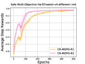
(a)

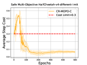
(b)

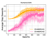
(c)

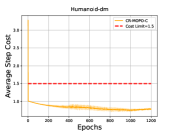
(d)

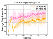
(e)

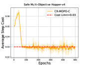
(f)

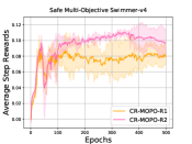
(g)

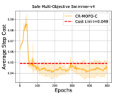
(h)

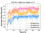
(i)

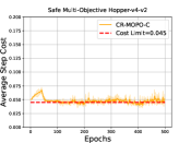
(j)

Figure 5: More Experiments to evaluate the effectiveness of our method on Safe Multi-Objective MuJoCo environments regarding the reward and safety performance.

Safe Multi-Objective HalfCheetah. As shown in Figure 4 (a), the constraint of Safe Multi-Objective halfCheetah is the difference between the robot real-time head height and the robot desired head height, as shown in Equation (30), $C_{h}^{i}$ denotes each step’s cost value, $H_{cheetah}^{i}$ denotes the real-time robot head’s height, $H_{target}^{i}$ denotes the target height. We set two reward functions for the robot’s two tasks. One reward is Energy saving. The robot needs to save Energy by optimizing its action, which means that to achieve the Goal, the robot needs to use the smallest Energy, $\alpha_{a}$ denotes the energy weight. As shown in Equation (32), $R_{e}^{i}$ denotes the action $a_{cheetah}^{i}$ energy at each step $i$. Another reward is velocity; the robot needs to achieve the velocity goal by learning to run as fast as possible. As shown in Equation (31), $R_{v}^{i}$ denotes each step’s velocity reward of the robot, $V_{cheetah}^{i}$ denotes the real-time each step’s velocity, $V_{target}^{i}$ denotes each step target velocity.

$$C_{h}^{i}=|H_{cheetah}^{i}-H_{target}^{i}|.$$ (30)

$$R_{v}^{i}=-|V_{cheetah}^{i}-V_{target}^{i}|.$$ (31)

$$R_{e}^{i}=-\alpha_{a}\|\textbf{$a_{cheetah}$}^{i}\|^{2}.$$ (32)

Safe Multi-Objective Hopper. As shown in Figure 4 (b), the constraint of Safe Multi-Objective Hopper is Energy that is computed via actions’ value, as shown in Equation (33), $C_{e-hopper}^{i}$ denotes the cost value. There are two objectives in the settings. The first reward function is the forward reward function, as shown in Equation (34). $R_{f}^{i}$ denotes the forward reward function, $\alpha_{v}$ denotes the forward reward weight, $X_{v}$ denotes the forward velocity. The second reward function is the healthy reward, e.g., the robot angle and state need to satisfy the requirements. As shown in Equation (35), $R_{he}^{i}$ denotes the healthy reward, and $R_{he-state}$ denotes the healthy state. This means the robot state needs to satisfy requirements; $R_{z}$ is the Z-axis robot healthy; $R_{angle}$ is the robot angle’s healthy. That is, the robot angle needs to satisfy the minimum and maximum angle requirements. Moreover, we modify reward settings as three objective tasks, named Safe Multi-Objective Hopper-v2, in which $R_{f}^{i},(R_{he-state}+R_{z}),R_{angle}$ are the three objective rewards respectively.

$$C_{e-hopper}^{i}=-\|\textbf{$a_{hopper}$}^{i}\|.$$ (33)

$$R_{f}^{i}=\alpha_{v}X_{V}.$$ (34)

$$R_{he}^{i}=R_{he-state}+R_{z}+R_{angle}.$$ (35)

$$R_{he-state}=\left\{\begin{aligned} 1&,&State_{min}\leq State_{real}\leq State_{max},\\ 0&,&Others.\end{aligned}\right.$$ (36)

$$R_{z}=\left\{\begin{aligned} 1&,&Z_{min}\leq Z_{real}\leq Z_{max},\\ 0&,&Others.\end{aligned}\right.$$ (37)

$$R_{angle}=\left\{\begin{aligned} 1&,&Angle_{min}\leq Angle_{real}\leq Angle_{max},\\ 0&,&Others.\end{aligned}\right.$$ (38)

Safe Multi-Objective Humanoid. As shown in Figure 4 (c), the constraint of Safe Multi-Objective Humanoid is the control cost value regarding saving Energy, as shown in Equation (39), $C_{e-humanoid}^{i}$ denotes the cost value at each step $i$. The first reward is the forward reward regarding velocity, similar to Equation (34). The higher velocity, the better the forward reward. The second reward is the healthy reward, which is about the robot stand. Thus, the higher the axis-z direction height, the better the healthy reward, as shown in Equation (40), $R_{he}^{i}$ denotes the healthy reward value, $H_{z}^{i}$ denotes the X-axis direction height.

$$C_{e-humanoid}^{i}=-\|\textbf{$a_{humanoid}$}^{i}\|^{2}.$$ (39)

$$R_{he}^{i}=H_{z}^{i}.$$ (40)

Safe Multi-Objective Swimmer. As shown in Figure 4 (d), the constraint is about action Energy, as shown in Equation 41, $C_{e-swimmer}^{i}$ denotes the cost value at each step, $\alpha_{swimmer}$ denotes the cost weight, $a_{swimmer}^{i}$ denotes the action value. There are two reward functions in the environment. One is the move forward reward, which is about the X-axis direction velocity, as shown in Equation (42), $R_{x-v}^{i}$ denotes the Y-axis direction reward at each step $i$, $\alpha_{v}$ denotes the weight of X-axis velocity, $X_{V}$ denotes the X-axis velocity; another is the move left reward, which is about the Y-axis direction velocity, as shown in Equation (43), $R_{y-v}^{i}$ denotes the Y-axis direction reward at each step $i$, $Y_{V}$ denotes the Y-axis velocity. The higher the velocities, the better the reward.

$$C_{e-swimmer}^{i}=-\alpha_{swimmer}\|\textbf{$a_{swimmer}$}^{i}\|.$$ (41)

$$R_{x-v}^{i}=\alpha_{v}X_{V}.$$ (42)

$$R_{y-v}^{i}=Y_{V}.$$ (43)

Safe Multi-Objective Walker. As shown in Figure 4 (e), the constraint of Safe Multi-Objective Walker is about action Energy, as shown in Equation (44). The first reward function is about move forward reward, similar to Equation (42). The second reward function is about the healthy reward, e.g., healthy angle and healthy Z-axis height. as shown in Equation (45), and the settings of $R_{z}$ and $R_{angle}$ are similar to Equation (37) and Equation (38).

$$C_{e-walker}^{i}=-\|\textbf{$a_{walker}$}^{i}\|.$$ (44)

$$R_{he}^{i}=R_{z}+R_{angle}.$$ (45)

Safe Multi-Objective Pusher. As shown in Figure 4 (f), the constraint of the Safe Multi-Objective Pusher is about the action Energy, as shown in Equation (46), $C_{e-pusher}^{i}$ denotes the cost value of each step $i$, $a_{pusher}^{i}$ is the set of actions at each step $i$. The first reward function is about the targeting object to the goal’s position, as shown in Equation (47), $R_{goal-pusher}^{i}$ denotes the first reward, $D_{object-goal}^{i}$ denotes the distance from targeting object to goal position at each step $i$. The second reward function is about the robot’s end effector position to the targeting object’s position, as shown in Equation (48), $R_{object-pusher}^{i}$ denotes the second reward at each step $i$, $D_{robot-object}^{i}$ denotes the distance from the robot to the object at each step $i$.

$$C_{e-pusher}^{i}=\|\textbf{$a_{pusher}$}^{i}\|^{2}.$$ (46)

$$R_{goal-pusher}^{i}=-\|\textbf{$D_{object-goal}$}^{i}\|.$$ (47)

$$R_{object-pusher}^{i}=-\|\textbf{$D_{robot-object}$}^{i}\|.$$ (48)

B.2 Implementation Details

Tables 1 and 2 provide the safety-bound parameters and algorithm parameters used in the study. The server with 40 CPU cores (Intel® Xeon(R) Gold 5218R CPU @ 2.10GHz × 80) and 1 GTX-970 GPU (NVIDIA GeForce GTX 970/PCIe/SSE2) is used to run the experiments on a Ubuntu 18.04 system.

Environment	value
Safe Multi-Objective HalfCheetah-v4	0.1
Safe Multi-Objective Humanoid-v4	0.9
Safe Multi-Objective Walker-v4	0.03
Safe Multi-Objective Humanoid-dm	1.5
Safe Multi-Objective HalfCheetah-v4-different-limit	0.3
Safe Multi-Objective Hopper-v4	0.03
Safe Multi-Objective Swimmer-v4	0.049
Safe Multi-Objective Pusher-v4	0.49
Safe Multi-Objective Walker-dm	1.5
Safe Multi-Objective-v4- soft-v1	0.005

Table 1: Safety bound of each step used in the Safe Multi-Objective Environments.

Parameters	value	Parameters	value
gamma	0.995	tau	0.97
l2-reg	1e-3	kl	0.05
damping	1e-1	batch-size	16000
epoch	500	episode length	1000
grad-c	0.5	neural network	MLP
hidden layer dim	64	accept ratio	0.1
energy weight	1.0	forward reward weight	1.0

Table 2: Key hyparameters used in experiments.

References

• [1] Abbas Abdolmaleki, Sandy Huang, Leonard Hasenclever, Michael Neunert, Francis Song, Martina Zambelli, Murilo Martins, Nicolas Heess, Raia Hadsell, and Martin Riedmiller. A distributional view on multi-objective policy optimization. In International Conference on Machine Learning, pages 11–22. PMLR, 2020.
• [2] Joshua Achiam, David Held, Aviv Tamar, and Pieter Abbeel. Constrained policy optimization. In International conference on machine learning, pages 22–31. PMLR, 2017.
• [3] Alekh Agarwal, Sham M Kakade, Jason D Lee, and Gaurav Mahajan. On the theory of policy gradient methods: Optimality, approximation, and distribution shift. The Journal of Machine Learning Research, 22(1):4431–4506, 2021.
• [4] Felix Berkenkamp and Angela P Schoellig. Safe and robust learning control with gaussian processes. In 2015 European Control Conference (ECC), pages 2496–2501. IEEE, 2015.
• [5] Jalaj Bhandari, Daniel Russo, and Raghav Singal. A finite time analysis of temporal difference learning with linear function approximation. In Conference on learning theory, pages 1691–1692. PMLR, 2018.
• [6] Greg Brockman, Vicki Cheung, Ludwig Pettersson, Jonas Schneider, John Schulman, Jie Tang, and Wojciech Zaremba. Openai gym. arXiv preprint arXiv:1606.01540, 2016.
• [7] Arthur Charpentier, Romuald Elie, and Carl Remlinger. Reinforcement learning in economics and finance. Computational Economics, pages 1–38, 2021.
• [8] Yinlam Chow, Ofir Nachum, Edgar Duenez-Guzman, and Mohammad Ghavamzadeh. A lyapunov-based approach to safe reinforcement learning. Advances in neural information processing systems, 31, 2018.
• [9] Yinlam Chow, Ofir Nachum, Aleksandra Faust, Edgar Duenez-Guzman, and Mohammad Ghavamzadeh. Lyapunov-based safe policy optimization for continuous control. arXiv preprint arXiv:1901.10031, 2019.
• [10] Gal Dalal, Balázs Szörényi, Gugan Thoppe, and Shie Mannor. Finite sample analyses for td (0) with function approximation. In Proceedings of the AAAI Conference on Artificial Intelligence, volume 32, 2018.
• [11] Jean-Antoine Désidéri. Multiple-gradient descent algorithm (mgda) for multiobjective optimization. Comptes Rendus Mathematique, 350(5-6):313–318, 2012.
• [12] Nathan Fulton and André Platzer. Safe reinforcement learning via formal methods: Toward safe control through proof and learning. In Proceedings of the AAAI Conference on Artificial Intelligence, volume 32, 2018.
• [13] Shangding Gu, Guang Chen, Lijun Zhang, Jing Hou, Yingbai Hu, and Alois Knoll. Constrained reinforcement learning for vehicle motion planning with topological reachability analysis. Robotics, 11(4):81, 2022.
• [14] Shangding Gu, Alap Kshirsagar, Yali Du, Guang Chen, Jan Peters, and Alois Knoll. A human-centered safe robot reinforcement learning framework with interactive behaviors. Frontiers in Neurorobotics, 17, 2023.
• [15] Shangding Gu, Jakub Grudzien Kuba, Yuanpei Chen, Yali Du, Long Yang, Alois Knoll, and Yaodong Yang. Safe multi-agent reinforcement learning for multi-robot control. Artificial Intelligence, 319:103905, 2023.
• [16] Shangding Gu, Long Yang, Yali Du, Guang Chen, Florian Walter, Jun Wang, Yaodong Yang, and Alois Knoll. A review of safe reinforcement learning: Methods, theory and applications. arXiv preprint arXiv:2205.10330, 2022.
• [17] Sandy Huang, Abbas Abdolmaleki, Giulia Vezzani, Philemon Brakel, Daniel J Mankowitz, Michael Neunert, Steven Bohez, Yuval Tassa, Nicolas Heess, Martin Riedmiller, et al. A constrained multi-objective reinforcement learning framework. In Conference on Robot Learning, pages 883–893. PMLR, 2022.
• [18] J John. Vector optimization, theory, application, and extensions, 2004.
• [19] Sham M Kakade. A natural policy gradient. Advances in neural information processing systems, 14, 2001.
• [20] B Ravi Kiran, Ibrahim Sobh, Victor Talpaert, Patrick Mannion, Ahmad A Al Sallab, Senthil Yogamani, and Patrick Pérez. Deep reinforcement learning for autonomous driving: A survey. IEEE Transactions on Intelligent Transportation Systems, 23(6):4909–4926, 2021.
• [21] Jens Kober, J Andrew Bagnell, and Jan Peters. Reinforcement learning in robotics: A survey. The International Journal of Robotics Research, 32(11):1238–1274, 2013.
• [22] Torsten Koller, Felix Berkenkamp, Matteo Turchetta, and Andreas Krause. Learning-based model predictive control for safe exploration. In 2018 IEEE conference on decision and control (CDC), pages 6059–6066. IEEE, 2018.
• [23] Vitaly Kurin, Alessandro De Palma, Ilya Kostrikov, Shimon Whiteson, and Pawan K Mudigonda. In defense of the unitary scalarization for deep multi-task learning. Advances in Neural Information Processing Systems, 35:12169–12183, 2022.
• [24] Xiao Li and Calin Belta. Temporal logic guided safe reinforcement learning using control barrier functions. arXiv preprint arXiv:1903.09885, 2019.
• [25] Bo Liu, Xingchao Liu, Xiaojie Jin, Peter Stone, and Qiang Liu. Conflict-averse gradient descent for multi-task learning. Advances in Neural Information Processing Systems, 34:18878–18890, 2021.
• [26] Yongshuai Liu, Jiaxin Ding, and Xin Liu. Ipo: Interior-point policy optimization under constraints. In Proceedings of the AAAI conference on artificial intelligence, volume 34, pages 4940–4947, 2020.
• [27] Zahra Marvi and Bahare Kiumarsi. Safe reinforcement learning: A control barrier function optimization approach. International Journal of Robust and Nonlinear Control, 31(6):1923–1940, 2021.
• [28] Aviv Navon, Aviv Shamsian, Idan Achituve, Haggai Maron, Kenji Kawaguchi, Gal Chechik, and Ethan Fetaya. Multi-task learning as a bargaining game. In International Conference on Machine Learning, pages 16428–16446. PMLR, 2022.
• [29] Long Ouyang, Jeffrey Wu, Xu Jiang, Diogo Almeida, Carroll Wainwright, Pamela Mishkin, Chong Zhang, Sandhini Agarwal, Katarina Slama, Alex Ray, et al. Training language models to follow instructions with human feedback. Advances in Neural Information Processing Systems, 35:27730–27744, 2022.
• [30] Simone Parisi, Matteo Pirotta, and Jan Peters. Manifold-based multi-objective policy search with sample reuse. Neurocomputing, 263:3–14, 2017.
• [31] Simone Parisi, Matteo Pirotta, and Marcello Restelli. Multi-objective reinforcement learning through continuous pareto manifold approximation. Journal of Artificial Intelligence Research, 57:187–227, 2016.
• [32] John Schulman, Sergey Levine, Pieter Abbeel, Michael Jordan, and Philipp Moritz. Trust region policy optimization. In International conference on machine learning, pages 1889–1897. PMLR, 2015.
• [33] Yanan Sui, Alkis Gotovos, Joel Burdick, and Andreas Krause. Safe exploration for optimization with gaussian processes. In International conference on machine learning, pages 997–1005. PMLR, 2015.
• [34] Richard S Sutton, David McAllester, Satinder Singh, and Yishay Mansour. Policy gradient methods for reinforcement learning with function approximation. Advances in neural information processing systems, 12, 1999.
• [35] Yuval Tassa, Yotam Doron, Alistair Muldal, Tom Erez, Yazhe Li, Diego de Las Casas, David Budden, Abbas Abdolmaleki, Josh Merel, Andrew Lefrancq, et al. Deepmind control suite. arXiv preprint arXiv:1801.00690, 2018.
• [36] Chen Tessler, Daniel J Mankowitz, and Shie Mannor. Reward constrained policy optimization. In International Conference on Learning Representations, 2018.
• [37] Emanuel Todorov, Tom Erez, and Yuval Tassa. Mujoco: A physics engine for model-based control. In 2012 IEEE/RSJ international conference on intelligent robots and systems, pages 5026–5033. IEEE, 2012.
• [38] Matteo Turchetta, Felix Berkenkamp, and Andreas Krause. Safe exploration in finite markov decision processes with gaussian processes. Advances in Neural Information Processing Systems, 29, 2016.
• [39] Peter Vamplew, Richard Dazeley, Adam Berry, Rustam Issabekov, and Evan Dekker. Empirical evaluation methods for multiobjective reinforcement learning algorithms. Machine Learning, 84(1-2):51–80, 2011.
• [40] Simon Vandenhende, Stamatios Georgoulis, Wouter Van Gansbeke, Marc Proesmans, Dengxin Dai, and Luc Van Gool. Multi-task learning for dense prediction tasks: A survey. IEEE transactions on pattern analysis and machine intelligence, 44(7):3614–3633, 2021.
• [41] Nelson Vithayathil Varghese and Qusay H Mahmoud. A survey of multi-task deep reinforcement learning. Electronics, 9(9):1363, 2020.
• [42] Akifumi Wachi, Yanan Sui, Yisong Yue, and Masahiro Ono. Safe exploration and optimization of constrained mdps using gaussian processes. In Proceedings of the AAAI Conference on Artificial Intelligence, volume 32, 2018.
• [43] Runzhe Wu, Yufeng Zhang, Zhuoran Yang, and Zhaoran Wang. Offline constrained multi-objective reinforcement learning via pessimistic dual value iteration. Advances in Neural Information Processing Systems, 34:25439–25451, 2021.
• [44] Tengyu Xu, Yingbin Liang, and Guanghui Lan. Crpo: A new approach for safe reinforcement learning with convergence guarantee. In International Conference on Machine Learning, pages 11480–11491. PMLR, 2021.
• [45] Sherry Yang, Ofir Nachum, Yilun Du, Jason Wei, Pieter Abbeel, and Dale Schuurmans. Foundation models for decision making: Problems, methods, and opportunities. arXiv preprint arXiv:2303.04129, 2023.
• [46] Tsung-Yen Yang, Justinian Rosca, Karthik Narasimhan, and Peter J. Ramadge. Projection-based constrained policy optimization. In International Conference on Learning Representations, 2020.
• [47] Tianhe Yu, Saurabh Kumar, Abhishek Gupta, Sergey Levine, Karol Hausman, and Chelsea Finn. Gradient surgery for multi-task learning. Advances in Neural Information Processing Systems, 33:5824–5836, 2020.
• [48] Kaiqing Zhang, Alec Koppel, Hao Zhu, and Tamer Basar. Global convergence of policy gradient methods to (almost) locally optimal policies. SIAM Journal on Control and Optimization, 58(6):3586–3612, 2020.
• [49] Shiji Zhou, Wenpeng Zhang, Jiyan Jiang, Wenliang Zhong, Jinjie Gu, and Wenwu Zhu. On the convergence of stochastic multi-objective gradient manipulation and beyond. Advances in Neural Information Processing Systems, 35:38103–38115, 2022.