Bending-Neutral Deformations of Minimal Surfaces

Abstract

Minimal surfaces are ubiquitous in nature. Here they are considered as geometric objects that bear a deformation content. By refining the resolution of the surface deformation gradient afforded by the polar decomposition theorem, we identify a bending content and a class of deformations that leave it unchanged. These are the bending-neutral deformations, fully characterized by an integrability condition. We prove that (1) every minimal surface is transformed into a minimal surface by a bending-neutral deformation and (2) given two minimal surfaces, there is a bending-neutral deformation that maps one into the other. Thus, all minimal surfaces have indeed a universal bending content.

I Introduction

The universe is parsimonious: so says the title of a celebrated book [1], which among many other things contains a fascinating account on minimal surfaces (disguised as soap bubbles). The theory of plates and shells should make no exception to this universal rule. However, researchers are still debating the most appropriate kinematic measures of deformation that would enter the elastic energy functional in an intrinsic (direct) theory of these bodies. In the language of the book [2], an intrinsic theory represents plates and shells as truly two-dimensional bodies, with mass distributed on a surface $\mathscr{S}$ in three-dimensional Euclidean space $\mathscr{E}$. The following works provide but a partial sample of the current debate [3, 4, 5, 6, 7, 8, 9, 10].

Here we build on an earlier proposal for measures of pure bending of a surface $\mathscr{S}$ [7], which was formulated as an invariance requirement under the class of bending-neutral deformations. In this paper, we identify as bending content of $\mathscr{S}$ the geometric object (a vector field) left unchanged by these deformations.

We prove that all minimal surfaces share one and the same bending content, so that each non-planar minimal surface can be seen as the image of another non-planar minimal surface under a bending-neutral deformation. Thus, making it impossible to properly bend one minimal surface into another.

The paper is organized as follows. In Sect. II, to make our development self-contained, we collect a few results about surface tensor calculus that are used in the rest of the paper. In Sect. III, we lay out our kinematic analysis: we recall the definition of bending-neutral deformations and identify the bending content of a surface. In Sect. IV, we show how minimal surfaces are tightly connected by bending-neutral deformations, which tie together all members of this class of surfaces. Section V collects the conclusions of this work and a few comments on their possible bearing on the theory of plates and shells, which was our original motivation and remains our primary intent.

The paper is closed by two appendices, where we give details about proofs left out of the main text to ease the flow of our presentation. Two animations and a Maple script are also provided as supplementary material for the reader. The animations show motions traversing minimal surfaces: they visibly convey an impression of gliding instead of bending, in accord with the theory. The Maple script was used to generate the animations and can be modified by the reader to explore further minimal surfaces and their deformations.

II Glimpses of Surface Differential Calculus

To make our paper self-contained, we recall some basic notions of differential calculus on smooth surfaces in three-dimensional space, especially those playing a role in the development that follows.

Let $\mathscr{S}$ be a smooth, orientable surface in three-dimensional Euclidean space $\mathscr{E}$; it can be represented (at least locally) by a mapping of class $C^{2}$ defined on a domain $S\subset\mathbb{R}^{2}$ described by a system of coordinates. Here, however, we shall keep our discussion independent of any particular choice of coordinates.

A scalar field $\varphi:\mathscr{S}\to\mathbb{R}$ is differentiable at a point $p\in\mathscr{S}$, if for every curve $\mathcal{c}:t\mapsto\mathcal{c}(t)\in\mathscr{S}$ such that $\mathcal{c}(t_{0})=p$ there is a vector $\nabla\!_{\mathrm{s}}\varphi$ on the tangent plane $\mathscr{T}_{p}$ to $\mathscr{S}$ at $p$ such that

$$\left.\frac{\mathrm{d}}{\mathrm{d}t}\varphi(\mathcal{c}(t))\right|_{t=t_{0}}=\nabla\!_{\mathrm{s}}\varphi\cdot\bm{t},$$ (1)

where $\bm{t}$ is the unit tangent vector to $\mathcal{c}$ at $p$. We call $\nabla\!_{\mathrm{s}}\varphi$ the surface gradient of $\varphi$.

Equivalently, $\nabla\!_{\mathrm{s}}\varphi$ can be introduced by extending $\varphi$ in a three-dimensional neighborhood that contains $\mathscr{S}$ to a smooth function $\tilde{\varphi}$ such that $\tilde{\varphi}|_{\mathscr{S}}=\varphi$. Letting $\nabla\tilde{\varphi}$ denote the ordinary, three-dimensional gradient of $\tilde{\varphi}$, we can uniquely decompose it in its tangential and normal components relative to $\mathscr{S}$:

$$\nabla\tilde{\varphi}=\mathbf{P}(\bm{\nu})\nabla\tilde{\varphi}+(\nabla\tilde{\varphi}\cdot\bm{\nu})\bm{\nu},$$ (2)

where $\bm{\nu}$ is a selected unit normal to $\mathscr{S}$ at $p\in\mathscr{S}$ and $\mathbf{P}(\bm{\nu}):=\mathbf{I}-\bm{\nu}\otimes\bm{\nu}$ is the projection onto the tangent plane $\mathscr{T}_{p}$. We can then set

$$\nabla\!_{\mathrm{s}}\varphi:=\mathbf{P}(\bm{\nu})\nabla\tilde{\varphi}\quad\text{and}\quad\nabla\!_{\nu}\tilde{\varphi}:=\nabla\tilde{\varphi}\cdot\bm{\nu},$$ (3)

the former depending only on $\varphi$ and the latter on its extension $\tilde{\varphi}$. One can devise $\tilde{\varphi}$ so that $\nabla\!_{\nu}\tilde{\varphi}=0$, as in [12]: this is called a normal extension of $\varphi$. Here, we shall not make use of such a restricted class of extensions.

The advantage of defining $\nabla\!_{\mathrm{s}}\varphi$ as in (3) is that this definition is easily extended to higher derivatives. Denoting by the same symbol also the extension of $\varphi$ (no confusion can arise, as only the normal derivative depends on the extension), we have that

$$\nabla^{2}\!\!\!\!_{\mathrm{s}}\varphi:=\nabla[\nabla\varphi-(\nabla\varphi\cdot\bm{\nu})\bm{\nu}]\mathbf{P}(\bm{\nu}),$$ (4)

where $\nabla$ denotes the standard gradient. By expanding (4) and setting $\nabla\!_{\mathrm{s}}\bm{\nu}:=(\nabla\bm{\nu})\mathbf{P}(\bm{\nu})$, having also extended $\bm{\nu}$ out of $\mathscr{S}$, by use of (3), we arrive at

$$\nabla^{2}\!\!\!\!_{\mathrm{s}}\varphi=\mathbf{P}(\bm{\nu})(\nabla^{2}\!\varphi)\mathbf{P}(\bm{\nu})-(\nabla\!_{\nu}\varphi)\nabla\!_{\mathrm{s}}\bm{\nu}-\bm{\nu}\otimes(\nabla\!_{\mathrm{s}}\bm{\nu})(\nabla\!_{\mathrm{s}}\varphi).$$ (5)

Two consequences follow immediately from (5). First, $\nabla^{2}\!\!\!\!_{\mathrm{s}}\varphi$ clearly depends on the extension of $\varphi$ outside $\mathscr{S}$; an intrinsic definition can be achieved by resorting to normal extensions of $\varphi$. Second, since both $\nabla^{2}\varphi$ and the curvature tensor $\nabla\!_{\mathrm{s}}\bm{\nu}$, which at each point $p\in\mathscr{S}$ maps $\mathscr{T}_{p}$ into itself, are symmetric, the skew-symmetric part of $\nabla^{2}\!\!\!\!_{\mathrm{s}}\varphi$ does not generally vanish, but it is independent of the extension of $\varphi$,

$$\operatorname{skw}(\nabla^{2}\!\!\!\!_{\mathrm{s}}\varphi)=\operatorname{skw}[(\nabla\!_{\mathrm{s}}\bm{\nu})(\nabla\!_{\mathrm{s}}\varphi)\otimes\bm{\nu}],$$ (6)

which is both intrinsic and fully determined by $\nabla\!_{\mathrm{s}}\varphi$ and the curvature of $\mathscr{S}$ (see also [13, 14]). Letting the axial vector associated with the skew-symmetric part of $\nabla^{2}\!\!\!\!_{\mathrm{s}}\varphi$ be the surface curl of $\nabla\!_{\mathrm{s}}\varphi$, we can rewrite (6) as

$$\operatorname{curl}_{\mathrm{s}}\!\nabla\!_{\mathrm{s}}\varphi=\bm{\nu}\times(\nabla\!_{\mathrm{s}}\bm{\nu})(\nabla\!_{\mathrm{s}}\varphi).$$ (7)

More generally, for $\bm{h}$ a given tangential vector field of class $C^{1}$ on $\mathscr{S}$, (6) is replaced by

$$\operatorname{skw}(\nabla\!_{\mathrm{s}}\bm{h})=\operatorname{skw}((\nabla\!_{\mathrm{s}}\bm{\nu})\bm{h}\otimes\bm{\nu}).$$ (8)

Similarly, for a given surface second-rank tensor field $\mathbf{F}$ of class $C^{1}$ on $\mathscr{S}$ such that $\mathbf{F}\bm{\nu}=\bm{0}$,

$$\operatorname{skw}(\nabla\!_{\mathrm{s}}\mathbf{F})=\operatorname{skw}(\mathbf{F}(\nabla\!_{\mathrm{s}}\bm{\nu})\otimes\bm{\nu}),$$ (9)

where the skew-symmetric part is taken on the last two legs of the third-rank tensors involved.

Consider now a closed curve $\mathcal{c}$ over $\mathscr{S}$ and denote by $\mathcal{s}\subset\mathscr{S}$ the portion of $\mathscr{S}$ that it encloses. The circulation theorem (see, for example, [11, p. 243]) says that for a (not necessarily tangential) vector field $\bm{h}$ defined on $\mathscr{S}$ the following identity holds

$$\oint_{\mathcal{c}}\bm{h}\cdot\bm{t}\mathrm{d}s=\int_{\mathcal{s}}\operatorname{curl}_{\mathrm{s}}\!\bm{h}\cdot\bm{\nu}\mathrm{d}A,$$ (10)

where $\bm{t}$ is the unit tangent to $\mathcal{c}$ (oriented anti-clockwise relative to $\bm{\nu}$), $s$ is the arc-length measure along $\mathcal{c}$, and $A$ is the area measure on $\mathscr{S}$.

It readily follows from (10) and (7) that a sufficient and necessary condition for a surface vector field $\bm{h}$ to be the surface gradient of a scalar field $\varphi$ is that both $\bm{h}$ and $\operatorname{curl}_{\mathrm{s}}\!\bm{h}$ are tangential to $\mathscr{S}$ [15, p. 244]. Said differently, for a tangential surface vector field $\bm{h}$, (8) is also a sufficient integrability condition, which guarantees the existence (at least locally) of a scalar field $\varphi$ such that $\bm{h}=\nabla\!_{\mathrm{s}}\varphi$. Similarly, (9) is also a sufficient integrability condition for a surface second-rank tensor field $\mathbf{F}$ that annihilates the normal: it guarantees the existence of a surface vector field $\bm{h}$ such that $\mathbf{F}=\nabla\!_{\mathrm{s}}\bm{h}$.

Finally, we define the surface Laplacian as $\mathop{{}\bigtriangleup_{\mathrm{s}}\!}\nolimits\varphi:=\operatorname{div}_{\mathrm{s}}\nabla\!_{\mathrm{s}}\varphi$ and we shall say that a scalar function $\varphi$ of class $C^{2}$ on $\mathscr{S}$ such that $\mathop{{}\bigtriangleup_{\mathrm{s}}\!}\nolimits\varphi=0$ is surface harmonic.

III Bending-Neutral Deformations

In this section we are concerned with the kinematics of plates. We think of $\mathscr{S}$ as the image of the mid-surface of a plate $S\subset\mathbb{R}^{2}$ in the $(x_{1},x_{2})$ plane of a Cartesian frame $(\bm{e}_{1},\bm{e}_{2},\bm{e}_{3})$ under a deformation $\bm{f}:S\to\mathscr{E}$, which is assumed to be of class $C^{2}$ (see Fig. 1).

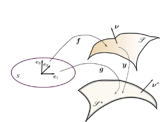
Figure 1: The surface $\mathscr{S}$ is obtained from the reference configuration $S$ in the $(x_{1},x_{2})$ plane of a Cartesian frame $(\bm{e}_{1},\bm{e}_{2},\bm{e}_{3})$ via the deformation $\bm{f}$. $\mathscr{S}^{\ast}$ is similarly obtained via the deformation $\bm{g}$. $\mathscr{S}$ is mapped onto $\mathscr{S}^{\ast}$ by the deformation $\bm{y}$; $\bm{\nu}$ and $\bm{\nu}^{\ast}$ are the unit vector fields that orient $\mathscr{S}$ and $\mathscr{S}^{\ast}$, respectively, while $\bm{e}_{3}$ is the unit normal orienting $S$.

In turn, $\mathscr{S}$ can be regarded as the reference configuration of a shell, which can be further deformed, as it will be at a later stage.

III.1 Kinematics

Letting $\bm{x}=x_{1}\bm{e}_{1}+x_{2}\bm{e}_{2}$ denote the position vector in $S$ and extending to the present geometric setting results well-known from three-dimensional kinematics (see, e.g., Chap. 6 of [17]), the deformation gradient $\nabla\bm{f}$ can be represented as

$$\nabla\bm{f}=\lambda_{1}\bm{b}_{1}\otimes\bm{c}_{1}+\lambda_{2}\bm{b}_{2}\otimes\bm{c}_{2},$$ (11)

where $\nabla$ denotes the gradient in $\bm{x}$, the positive scalars $\lambda_{1}$, $\lambda_{2}$ are the principal stretches and the unit vectors $\bm{c}_{i}$, $\bm{b}_{i}$ are the corresponding right and left principal directions of stretching. While $\bm{c}_{1}(\bm{x})$ and $\bm{c}_{2}(\bm{x})$ live on the $(\bm{e}_{1},\bm{e}_{2})$ plane for all $\bm{x}\in S$, $\bm{b}_{1}(\bm{x})$ and $\bm{b}_{2}(\bm{x})$ live on the tangent plane $\mathscr{T}_{\bm{f}(\bm{x})}$ to $\mathscr{S}$ at $\bm{f}(\bm{x})$. The right and left Cauchy-Green tensors are correspondingly given by

$$\mathbf{C}_{\bm{f}} :=(\nabla\bm{f})^{\mathsf{T}}(\nabla\bm{f})=\lambda_{1}^{2}\bm{c}_{1}\otimes\bm{c}_{1}+\lambda_{2}^{2}\bm{c}_{2}\otimes\bm{c}_{2},$$ (12a)

$$\mathbf{B}_{\bm{f}} :=(\nabla\bm{f})(\nabla\bm{f})^{\mathsf{T}}=\lambda_{1}^{2}\bm{b}_{1}\otimes\bm{b}_{1}+\lambda_{2}^{2}\bm{b}_{2}\otimes\bm{b}_{2}.$$ (12b)

By the polar decomposition theorem for the deformation of surfaces established in [18] within the general coordinate-free theory introduced in [19] (see also [20]), the deformation gradient $\nabla\bm{f}$ can be written as

$$\nabla\bm{f}=\mathbf{R}_{\bm{f}}\mathbf{U}_{\bm{f}}=\mathbf{V}_{\bm{f}}\mathbf{R}_{\bm{f}},$$ (13)

where $\mathbf{R}_{\bm{f}}$ is a rotation of the special orthogonal group in three dimensions $\mathsf{SO}(3)$ and

$$\mathbf{U}_{\bm{f}}=\lambda_{1}\bm{c}_{1}\otimes\bm{c}_{1}+\lambda_{2}\bm{c}_{2}\otimes\bm{c}_{2}\quad\text{and}\quad\mathbf{V}_{\bm{f}}=\lambda_{1}\bm{b}_{1}\otimes\bm{b}_{1}+\lambda_{2}\bm{b}_{2}\otimes\bm{b}_{2}$$ (14)

are the stretching tensors. It readily follows from (13) that $\bm{b}_{i}=\mathbf{R}_{\bm{f}}\bm{c}_{i}$.

III.2 Bending and drilling rotations

In (13), the rotation $\mathbf{R}_{\bm{f}}$, which can be different at different places $\bm{x}$, represents the non-metric component of the deformation $\bm{f}$. It follows from Euler’s theorem on rotations (see, for example, [21] for a modern discussion) that for every $\mathbf{R}\in\mathsf{SO}(3)$ there is an axis, designated by a unit vector $\bm{e}\in\mathbb{S}^{2}$, and a scalar $\alpha\in[0,\pi]$ such that $\mathbf{R}$ is a (conventionally anticlockwise) rotation about $\bm{e}$ by angle $\alpha$. More precisely, the following representation applies,

$$\mathbf{R}=\mathbf{I}+\sin\alpha\mathbf{W}(\bm{e})+(1-\cos\alpha)\mathbf{W}(\bm{e})^{2},$$ (15)

where $\mathbf{I}$ is the identity tensor, $\mathbf{W}(\bm{e})$ is the skew-symmetric tensor associated with $\bm{e}$ (so that $\mathbf{W}(\bm{e})\bm{v}=\bm{e}\times\bm{v}$ for all vectors $\bm{v}$). $\mathsf{SO}(3)$ is set by (15) into a one-to-one correspondence with the ball $\mathbb{B}^{3}_{\pi}\subset\mathscr{E}$ of radius $\pi$ centred at the origin. This latter corresponds to the identity $\mathbf{I}$, whereas the points on $\partial\mathbb{B}^{3}_{\pi}$ are $\pi$-turns, that is, rotations by an angle $\pi$, which are the only symmetric members of $\mathsf{SO}(3)$ other than $\mathbf{I}$.

As shown in Appendix A, $\mathbf{R}_{\bm{f}}$ can be uniquely decomposed into two rotations, $\mathbf{R}_{\bm{f}}^{(\mathrm{d})}$ with axis along the normal $\bm{e}_{3}$ to $S$ and $\mathbf{R}_{\bm{f}}^{(\mathrm{b})}$ with axis in the $(\bm{e}_{1},\bm{e}_{2})$ plane. We shall interpret $\mathbf{R}_{\bm{f}}^{(\mathrm{b})}$ as the bending content of $\mathbf{R}_{\bm{f}}$ and $\mathbf{R}_{\bm{f}}^{(\mathrm{d})}$ as the drilling content. Formally, we write

$$\mathbf{R}_{\bm{f}}=\mathbf{R}_{\bm{f}}^{(\mathrm{b})}\mathbf{R}_{\bm{f}}^{(\mathrm{d})},$$ (16)

where the order of composition matters, as bending and drilling rotations are about different axes. A pure drilling rotation, for which $\mathbf{R}_{\bm{f}}^{(\mathrm{b})}$ is uniform but $\mathbf{R}_{\bm{f}}^{(\mathrm{d})}$ is not, would pertain to a deformation $\bm{f}$ that strains $S$ but leaves it planar. A pure bending rotation, for which $\mathbf{R}_{\bm{f}}^{(\mathrm{d})}$ is uniform but $\mathbf{R}_{\bm{f}}^{(\mathrm{b})}$ is not, would instead pertain to a deformation $\bm{f}$ that brings $S$ out of a plane.

To identify both $\mathbf{R}_{\bm{f}}^{(\mathrm{d})}$ and $\mathbf{R}_{\bm{f}}^{(\mathrm{b})}$ for a given $\mathbf{R}_{\bm{f}}$, it is expedient to represent a member $\mathbf{R}\in\mathsf{SO}(3)$ via Rodrigues’ formula,

$$\mathbf{R}(\bm{a})=\frac{1}{1+a^{2}}\left\{(1-a^{2})\mathbf{I}+2\bm{a}\otimes\bm{a}+2\mathbf{W}(\bm{a})\right\},$$ (17)

where $\bm{a}$ is a vector of arbitrary length $a:=\sqrt{\bm{a}\cdot\bm{a}}$. This is the vector representation of a rotation, where $\mathsf{SO}(3)$ is set into a one-to-one correspondence with the whole translation space $\mathscr{V}$ of $\mathscr{E}$: the identity is still represented by the origin, but here $\pi$-turns are points at infinity.

Equation (17) follows from (15) by setting $\bm{a}=\tan(\alpha/2)\bm{e}$ and remarking that $\mathbf{W}(\bm{e})^{2}=-\mathbf{I}+\bm{e}\otimes\bm{e}$. It can also be easily inverted: for given $\mathbf{R}\in\mathsf{SO}(3)$, the representing vector $\bm{a}$ is identified by

$$\mathbf{W}(\bm{a})=\frac{\mathbf{R}-\mathbf{R}^{\mathsf{T}}}{1+\operatorname{tr}\mathbf{R}},$$ (18)

whence

$$a^{2}=\frac{3-\operatorname{tr}\mathbf{R}}{1+\operatorname{tr}\mathbf{R}},$$ (19)

which shows that a $\pi$-turn is characterized by having $\operatorname{tr}\mathbf{R}=-1$.

Rodrigues [26] proved a composition formula, which in modern terms can be phrased as follows (see, for example, also [27]): for $\mathbf{R}(\bm{a}_{1})$ and $\mathbf{R}(\bm{a}_{2})$ in $\mathsf{SO}(3)$ represented as in (17),

$$\mathbf{R}(\bm{a}_{2})\mathbf{R}(\bm{a}_{1})=\mathbf{R}(\bm{a}),$$ (20)

where

$$\bm{a}=\frac{\bm{a}_{1}+\bm{a}_{2}+\bm{a}_{2}\times\bm{a}_{1}}{1-\bm{a}_{1}\cdot\bm{a}_{2}}.$$ (21)

In particular, (21) shows that the composed rotation $\mathbf{R}(\bm{a})$ is a $\pi$-turn whenever $\bm{a}_{1}$ and $\bm{a}_{2}$ belong to the cone defined by $\bm{a}_{1}\cdot\bm{a}_{2}=1$.

Let $\mathbf{R}(\bm{a})$ be given in $\mathsf{SO}(3)$; we prove in Appendix A that it can uniquely be decomposed as in (20) into a rotation $\mathbf{R}(\bm{a}_{1})$ with $\bm{a}_{1}$ parallel to a given unit vector $\bm{e}$ and a rotation $\mathbf{R}(\bm{a}_{2})$ with $\bm{a}_{2}$ orthogonal to $\bm{e}$. The vectors $\bm{a}_{1}$ and $\bm{a}_{2}$ are explicitly determined as

$$\bm{a}_{1}=(\bm{a}\cdot\bm{e})\bm{e},\quad\bm{a}_{2}=\frac{1}{1+(\bm{a}\cdot\bm{e})^{2}}\{\mathbf{I}+(\bm{a}\cdot\bm{e})\mathbf{W}(\bm{e})\}\mathbf{P}(\bm{e})\bm{a},$$ (22)

where $\mathbf{P}(\bm{e}):=\mathbf{I}-\bm{e}\otimes\bm{e}$ is the projector on the plane orthogonal to $\bm{e}$. It easily follows from (22) that

$$a_{1}^{2}=(\bm{a}\cdot\bm{e})^{2}\quad\text{and}\quad a_{2}^{2}=\frac{a^{2}-a_{1}^{2}}{1+a_{1}^{2}}.$$ (23)

It is interesting to note that the rotation $\mathbf{R}(\bm{a}_{1})$ just determined can also be characterized as the member in the subgroup $\mathsf{SO}(\bm{e})\subset\mathsf{SO}(3)$ of all rotations with axis $\bm{e}$ that is the closest to $\mathbf{R}(\bm{a})$ in the sense made precise in Appendix A, where this result is proved in detail.

For $\mathbf{R}_{\bm{f}}\in\mathsf{SO}(3)$, we set $\mathbf{R}_{\bm{f}}^{(\mathrm{d})}:=\mathbf{R}(\bm{d}_{\bm{f}})$ and $\mathbf{R}_{\bm{f}}^{(\mathrm{b})}:=\mathbf{R}(\bm{b}_{\bm{f}})$, where, repeating (22) verbatim,

$$\bm{d}_{\bm{f}}=(\bm{a}_{\bm{f}}\cdot\bm{e}_{3})\bm{e}_{3},\quad\bm{b}_{\bm{f}}=\frac{1}{1+(\bm{a}_{\bm{f}}\cdot\bm{e}_{3})^{2}}\{\mathbf{I}+(\bm{a}_{\bm{f}}\cdot\bm{e}_{3})\mathbf{W}(\bm{e}_{3})\}\mathbf{P}(\bm{e}_{3})\bm{a}_{\bm{f}},$$ (24)

and $\bm{a}_{\bm{f}}$ is the vector associated with $\mathbf{R}_{\bm{f}}$ via (17), so that (16) applies.

III.3 Bending neutrality

We wish to identify a class of deformations that do not alter the bending content of a surface $\mathscr{S}$ (relative to its flat reference configuration $S$). Let $\mathscr{S}$ be obtained as above from $S$ via the deformation $\bm{f}$ and let $\bm{y}:\mathscr{S}\to\mathscr{E}$ be a deformation of $\mathscr{S}$ that transforms it into $\mathscr{S}^{\ast}$ (see Fig. 1). We say that $\bm{y}$ is a bending-neutral deformation if

$$\mathbf{R}_{\bm{y}}=\mathbf{R}_{\bm{\nu}}\in\mathsf{SO}(\bm{\nu})\quad\text{on}\ \mathscr{S},$$ (25)

where $\bm{\nu}$ is the unit normal to $\mathscr{S}$ oriented coherently with the orientation of $S$. This amounts to require that the bending component $\mathbf{R}_{\bm{y}}^{(\mathrm{b})}$ of $\bm{y}$ be any uniform rotation $\mathbf{R}_{0}$, which can always be chosen to be the identity $\mathbf{I}$ by an appropriate change of observer.

The surface $\mathscr{S}^{\ast}$ can also be regarded as the image of $S$ under the deformation $\bm{g}:=\bm{y}\circ\bm{f}$. We now show that for every bending-neutral deformation $\bm{y}$ of $\mathscr{S}$ the deformations $\bm{g}$ and $\bm{f}$ have one and the same bending content. To this end, we first remark that the unit normal $\bm{\nu}$ at $\bm{f}(\bm{x})$ is given by

$$\bm{\nu}=\frac{(\nabla\bm{f})\bm{e}_{1}\times(\nabla\bm{f})\bm{e}_{2}}{|{(\nabla\bm{f})\bm{e}_{1}\times(\nabla\bm{f})\bm{e}_{2}}|}=\frac{\operatorname{co}(\nabla\bm{f})\bm{e}_{3}}{|\operatorname{co}(\nabla\bm{f})\bm{e}_{3}|},$$ (26)

where $\operatorname{co}(\cdot)$ denotes the cofactor tensor (a definition is given, for exmaple, in Sect. 2.11 of [17]). Since, for any two tensors $\mathbf{L}$ and $\mathbf{M}$, $\operatorname{co}(\mathbf{L}\mathbf{M})=\operatorname{co}(\mathbf{L})\operatorname{co}(\mathbf{M})$ and $\operatorname{co}(\mathbf{R})=\mathbf{R}$ for all $\mathbf{R}\in\mathsf{SO}(3)$, it follows from (13) and (26) that

$$\bm{\nu}(\bm{f}(\bm{x}))=\mathbf{R}_{\bm{f}}\bm{e}_{3}\quad\forall\ \bm{x}\in S,$$ (27a)

as, by (14), $$\operatorname{co}(\mathbf{U}_{\bm{f}})=(\det\mathbf{U}_{\bm{f}})\bm{e}_{3}\otimes\bm{e}_{3} \bm{\nu}^{\ast} \mathscr{S}^{\ast}$$. Similarly, denoting by the unit normal to , we also have that

$$\bm{\nu}^{\ast}(\bm{g}(\bm{x}))=\mathbf{R}_{\bm{g}}\bm{e}_{3}\quad\forall\ \bm{x}\in S.$$ (27b)

On the other hand, since $\mathscr{S}^{\ast}=\bm{y}(\mathscr{S})$,

$$\bm{\nu}^{\ast}(\bm{\xi})=\frac{\operatorname{co}(\nabla\!_{\mathrm{s}}\bm{y})\bm{\nu}}{|\operatorname{co}(\nabla\!_{\mathrm{s}}\bm{y})\bm{\nu}|}\quad\forall\ \bm{\xi}\in\mathscr{S}$$ (28)

and decomposing $(\nabla\!_{\mathrm{s}}\bm{y})$ as $\nabla\!_{\mathrm{s}}\bm{y}=\mathbf{R}_{\bm{y}}\mathbf{U}_{\bm{y}}$, where

$$\mathbf{U}_{\bm{y}}(\bm{\xi})=\mu_{1}\bm{u}_{1}\otimes\bm{u}_{1}+\mu_{2}\bm{u}_{2}\otimes\bm{u}_{2}\quad\text{with}\quad\mu_{1},\mu_{2}>0$$ (29)

is the surface stretching tensor represented in its eigenframe $(\bm{u}_{1},\bm{u}_{2})$ on the tangent plane $\mathscr{T}_{\bm{\xi}}$ to $\mathscr{S}$, we see that $\bm{\nu}^{\ast}=\mathbf{R}_{\bm{y}}\bm{\nu}$, as $\operatorname{co}(\mathbf{U}_{\bm{y}})=(\det\mathbf{U}_{\bm{y}})\bm{\nu}\otimes\bm{\nu}$. Then (25) implies that $\bm{\nu}^{\ast}(\bm{g}(\bm{x}))=\bm{\nu}(\bm{f}(\bm{x}))$ for all $\bm{x}\in S$, which by (27) and (17) amounts to the equation

$$(\bm{b}_{\bm{f}}-\bm{b}_{\bm{g}})\times\bm{e}_{3}=\bm{0}\quad\Rightarrow\quad\bm{b}_{\bm{f}}=\bm{b}_{\bm{g}}=\bm{b}\quad\text{since}\quad\bm{b}_{\bm{f}}\cdot\bm{e}_{3}=\bm{b}_{\bm{g}}\cdot\bm{e}_{3}=0.$$ (30)

This is the desired result, which justifies our identifying the vector $\bm{b}$ as the bending content common to all surfaces related via a bending-neutral deformation.

The definition of bending-neutral deformations was introduced in [7] in an attempt to provide a solid foundation to the notion of pure measures of bending in plate theory. These were defined as deformation measures (either scalars or tensors) invariant under the action of all bending-neutral deformations. For example, it was shown in [7] that the tensor

$$\mathbf{A}:=(\nabla\bm{\nu})^{\mathsf{T}}(\nabla\bm{\nu})$$ (31)

is a pure measure of bending, whereas the tensor $\mathbf{K}:=(\nabla\bm{\nu})(\nabla\bm{\nu})^{\mathsf{T}}$ is not, even if it shares with $\mathbf{A}$ all scalar invariants.

III.4 Compatibility condition

The existence of a bending-neutral deformation is subject to a compatibility condition that involves the curvature of $\mathscr{S}$: as shown in [7], the rotation $\mathbf{R}_{\bm{\nu}}$ and the surface stretching $\mathbf{U}_{\bm{y}}$ that decompose $\nabla\!_{\mathrm{s}}\bm{y}$ must be such that

$$\nabla\!_{\mathrm{s}}\bm{\nu}=\mathbf{R}_{\bm{\nu}}\mathbf{U}_{\bm{y}}^{-1}(\nabla\!_{\mathrm{s}}\bm{\nu})\mathbf{R}_{\bm{\nu}}\mathbf{U}_{\bm{y}}.$$ (32)

This condition ensures that the tensor $\nabla\!_{\mathrm{s}}\bm{\nu}^{\ast}$ be symmetric, as it should. We represent $\nabla\!_{\mathrm{s}}\bm{\nu}$ as

$$\nabla\!_{\mathrm{s}}\bm{\nu}=\kappa_{1}\bm{n}_{1}\otimes\bm{n}_{1}+\kappa_{2}\bm{n}_{2}\otimes\bm{n}_{2},$$ (33)

where $(\kappa_{1},\kappa_{2})$ are the principal curvatures of $\mathscr{S}$ and $(\bm{n}_{1},\bm{n}_{2})$ the corresponding principal directions of curvature, and we let $\beta$ be the angle the eigenframe $(\bm{n}_{1},\bm{n}_{2})$ of $\nabla\!_{\mathrm{s}}\bm{\nu}$ makes with the eigenframe $(\bm{u}_{1},\bm{u}_{2})$ of $\mathbf{U}_{\bm{y}}$ in (29). By writing $\mathbf{R}_{\bm{\nu}}$ as in (15),

$$\mathbf{R}_{\bm{\nu}}(\alpha)=\mathbf{I}+\sin\alpha\mathbf{W}(\bm{\nu})-(1-\cos\alpha)\mathbf{P}(\bm{\nu})\quad\text{with}\quad\alpha\in[-\pi,\pi],$$ (34)

equation (32) can then be reduced to a single scalar equation, see [7],

$$\frac{\mu_{2}}{\mu_{1}}=1-\frac{(\kappa_{1}+\kappa_{2})\sin\alpha}{\kappa_{2}\sin\alpha+(\kappa_{1}-\kappa_{2})\cos\beta\sin(\alpha+\beta)},$$ (35)

which is thus the general compatibility condition for the existence of a bending-neutral deformation of $\mathscr{S}$. Since only the ratio between the principal surface stretches is prescribed by (35), $\mathbf{U}_{\bm{y}}$ can only determined to within a multiplicative surface dilation $\lambda\mathbf{P}(\bm{\nu})$, with $\lambda$ an arbitrary positive scalar field on $\mathscr{S}$.

A special class of solutions of (35) is obtained for $\beta=0$ and $\alpha\notin\{0,\pi\}$. This requires $\mathscr{S}$ to be a hyperbolic surface, that is, such that the Gaussian curvature $K:=\kappa_{1}\kappa_{2}<0$, as (35) reduces to

$$\frac{\mu_{2}}{\mu_{1}}=-\frac{\kappa_{2}}{\kappa_{1}}>0.$$ (36)

In this class of solutions of (35), $\mathbf{U}_{\bm{y}}$ can be represented as

$$\mathbf{U}_{\bm{y}}=\lambda(\kappa_{1}\bm{n}_{1}\otimes\bm{n}_{1}-\kappa_{2}\bm{n}_{2}\otimes\bm{n}_{2}).$$ (37)

It is not restrictive to assume that both $\kappa_{1}>0$ and $\lambda>0$. As proved in [7], for $\mathbf{U}_{\bm{y}}$ as in (37), the curvature tensor of $\mathscr{S}^{\ast}$ can be written as

$$\nabla\!_{\mathrm{s}}\bm{\nu}^{\ast}=\frac{\kappa_{1}}{\mu_{1}}\bm{n}_{1}\otimes\mathbf{R}_{\bm{\nu}}\bm{n}_{1}+\frac{\kappa_{2}}{\mu_{2}}\bm{n}_{2}\otimes\mathbf{R}_{\bm{\nu}}\bm{n}_{2},$$ (38)

which, by (34) and (36), implies that the total curvature of $\mathscr{S}^{\ast}$ is

$$2H^{\ast}:=\operatorname{tr}(\nabla\!_{\mathrm{s}}\bm{\nu}^{\ast})=\cos\alpha\left(\frac{\kappa_{1}}{\mu_{1}}+\frac{\kappa_{2}}{\mu_{2}}\right)=0.$$ (39)

Thus, if there exists a bending-neutral deformation $\bm{y}$ of a hyperbolic surface $\mathscr{S}$ with stretching tensor $\mathbf{U}_{\bm{y}}$ as in (37), it necessarily maps $\mathscr{S}$ into a minimal surface $\mathscr{S}^{\ast}$.

III.5 Integrability condition

Having solved (in a special case) the compatibility condition (32), we found a class of possible bending-neutral deformations $\bm{y}$ of a hyperbolic surface $\mathscr{S}$ characterized by

$$\nabla\!_{\mathrm{s}}\bm{y}=\mathbf{R}_{\bm{\nu}}(\alpha)\mathbf{U}_{\bm{y}},$$ (40)

where $\mathbf{U}_{\bm{y}}$ is given by (37) and both $\lambda$ and $\alpha$ are surface fields to be determined. However, there is no guarantee that (40) actually represents a surface gradient. For this to be the case, the tensor field $\mathbf{F}:=\mathbf{R}_{\bm{\nu}}(\alpha)\mathbf{U}_{\bm{y}}$ must satisfy the integrability condition (9). It is shown in Appendix B that (9) is satisfied if and only if $\lambda$ and $\alpha$ obey the following system of equations,

$$\begin{cases}\nabla\!_{\mathrm{s}}(\lambda\kappa_{1}\cos\alpha)\cdot\bm{n}_{2}-\nabla\!_{\mathrm{s}}(\lambda\kappa_{2}\sin\alpha)\cdot\bm{n}_{1}=\lambda(\kappa_{1}+\kappa_{2})(\cos\alpha\,\bm{c}\cdot\bm{n}_{1}+\sin\alpha\,\bm{c}\cdot\bm{n}_{2}),\\ \nabla\!_{\mathrm{s}}(\lambda\kappa_{1}\sin\alpha)\cdot\bm{n}_{2}+\nabla\!_{\mathrm{s}}(\lambda\kappa_{2}\cos\alpha)\cdot\bm{n}_{1}=\lambda(\kappa_{1}+\kappa_{2})(\sin\alpha\,\bm{c}\cdot\bm{n}_{1}-\cos\alpha\,\bm{c}\cdot\bm{n}_{2}),\end{cases}$$ (41)

where $\bm{c}$ is the Cartesian connector field defined as

$$\bm{c}:=(\nabla\!_{\mathrm{s}}\bm{n}_{1})^{\mathsf{T}}\bm{n}_{2}=-(\nabla\!_{\mathrm{s}}\bm{n}_{2})^{\mathsf{T}}\bm{n}_{1}.$$ (42)

The system (41) acquires a more compact form when $\mathscr{S}$ itself is a minimal surface,

$$\nabla\!_{\mathrm{s}}(\mu\sin\alpha)=\bm{\nu}\times\nabla\!_{\mathrm{s}}(\mu\cos\alpha),$$ (43)

where $\mu:=\lambda\kappa>0$ and $\kappa:=\kappa_{1}=-\kappa_{2}$, so that (40) reduces to

$$\nabla\!_{\mathrm{s}}\bm{y}=\mu\mathbf{R}_{\bm{\nu}}(\alpha)\mathbf{P}(\bm{\nu}).$$ (44)

It follows from (43) that

$$\begin{cases}\nabla\!_{\mathrm{s}}(\mu\sin\alpha)\cdot\nabla\!_{\mathrm{s}}(\mu\cos\alpha)=0,\\ |\nabla\!_{\mathrm{s}}(\mu\sin\alpha)|=|\nabla\!_{\mathrm{s}}(\mu\cos\alpha)|.\end{cases}$$ (45)

Expanding this system, we arrive at

$$\begin{cases}\mu\nabla\!_{\mathrm{s}}\mu\cdot\nabla\!_{\mathrm{s}}\alpha=0,\\ |\nabla\!_{\mathrm{s}}\mu|^{2}=\mu^{2}|\nabla\!_{\mathrm{s}}\alpha|^{2},\end{cases}$$ (46)

which amounts to the alternative $\nabla\!_{\mathrm{s}}\mu=\pm\mu\bm{\nu}\times\nabla\!_{\mathrm{s}}\alpha$. Insertion of either forms in (43) shows that the latter is only solved by $\nabla\!_{\mathrm{s}}\mu=-\mu\bm{\nu}\times\nabla\!_{\mathrm{s}}\alpha$, which can equivalently be written as

$$\nabla\!_{\mathrm{s}}\alpha=\bm{\nu}\times\nabla\!_{\mathrm{s}}\varphi,$$ (47)

where we have set $\varphi:=\ln\mu$.

As recalled in Sect. II, for (47) to be integrable, the field $\bm{h}=\bm{\nu}\times\nabla\!_{\mathrm{s}}\varphi$, which is tangential to $\mathscr{S}$, must also be such that $\operatorname{curl}_{\mathrm{s}}\!\bm{h}\cdot\bm{\nu}=0$. For $\varphi$ of class $C^{2}$, we easily see that

$$\operatorname{curl}_{\mathrm{s}}\!\bm{h}=(\nabla\!_{\mathrm{s}}\bm{\nu})\nabla\!_{\mathrm{s}}\varphi-(\nabla^{2}\!\!\!\!_{\mathrm{s}}\varphi)\bm{\nu}+(\mathop{{}\bigtriangleup_{\mathrm{s}}\!}\nolimits\varphi)\bm{\nu}-(\operatorname{div}_{\mathrm{s}}\bm{\nu})\nabla\!_{\mathrm{s}}\varphi,$$ (48)

where $\operatorname{div}_{\mathrm{s}}\bm{\nu}:=\operatorname{tr}(\nabla\!_{\mathrm{s}}\bm{\nu})=2H$ is the total curvature of $\mathscr{S}$, which vanishes for a minimal surface. By use of (5) in (48), we conclude that $\operatorname{curl}_{\mathrm{s}}\!\bm{h}\cdot\bm{\nu}=0$ whenever

$$\mathop{{}\bigtriangleup_{\mathrm{s}}\!}\nolimits\varphi=0.$$ (49)

Thus, for any surface harmonic function $\varphi$ on $\mathscr{S}$, we can set $\mu=\exp(\varphi)$ in (44). Correspondingly, (47) is integrable and it too delivers a surface harmonic function $\alpha$, as it implies that, for $\alpha$ of class $C^{2}$,

$$\mathop{{}\bigtriangleup_{\mathrm{s}}\!}\nolimits\alpha=\operatorname{curl}_{\mathrm{s}}\!\bm{\nu}\cdot\nabla\!_{\mathrm{s}}\varphi-\bm{\nu}\cdot\operatorname{curl}_{\mathrm{s}}\!\nabla\!_{\mathrm{s}}\varphi=0$$ (50)

because $\operatorname{curl}_{\mathrm{s}}\!\bm{\nu}=\bm{0}$, by the symmetry of the curvature tensor. This identifies (at least locally) a drilling rotation $\mathbf{R}_{\bm{\nu}}$ that makes equation (44) integrable, so as to determine locally (to within a translation) a bending-neutral deformation of $\mathscr{S}$. We have actually found a whole class of bending-neutral deformations of $\mathscr{S}$, each represented by a surface harmonic function $\varphi$ on $\mathscr{S}$.

We shall see in the following section that this bond between bending-neutral deformations of minimal surfaces and surface harmonic functions is indeed much stronger.

IV Minimal Surfaces

Here we show that every two minimal surfaces of class $C^{2}$ are one the image of the other under a bending-neutral deformation in the family described in Sect. III. To this end, it is particularly instrumental to resort to the celebrated Enneper-Weierstrass representation of minimal surfaces (see, for example, Sect. 3.3 of [34]), which requires the use of isothermal parameters $(u,v)$ to describe a surface $\mathscr{S}$.

In an isothermal parameterization, the mapping $\bm{r}:\Omega\to\mathscr{E}$ that represents $\mathscr{S}$ as image of a simply connected set $\Omega$ of the $(u,v)$ plane enjoys the following properties,

$$|\bm{r}_{,u}|=|\bm{r}_{,v}|\quad\text{and}\quad\bm{r}_{,u}\cdot\bm{r}_{,v}=0,$$ (51)

where a comma denotes differentiation. Moreover, since also

$$\mathop{{}\bigtriangleup}\nolimits\bm{r}=\bm{r}_{,uu}+\bm{r}_{,vv}=\bm{0}$$ (52)

(see, for example, [37, p. 268]), for any scalar-valued function $\varphi$ defined on $\mathscr{S}$ in terms of the $(u,v)$ parameters,

$$\mathop{{}\bigtriangleup_{\mathrm{s}}\!}\nolimits\varphi=\frac{1}{|\bm{r}_{,u}|^{2}}\mathop{{}\bigtriangleup}\nolimits\varphi=\frac{1}{|\bm{r}_{,u}|^{2}}(\varphi_{,uu}+\varphi_{,vv}),$$ (53)

so that $\varphi$ is surface harmonic on $\mathscr{S}$ whenever it is harmonic in $\Omega$.

IV.1 Weierstrass representation

Let $w:=u+iv\in\mathbb{C}$ be a complex representation of the $(u,v)$ plane. A minimal surface $\mathscr{S}$ such that the normal $\bm{\nu}$ regarded as a map from $\Omega$ into the unit sphere $\mathbb{S}^{2}$ is injective, but does not cover the whole of $\mathbb{S}^{2}$, can be represented (to within a translation) by a holomorphic function $F:\Omega\to\mathbb{C}$ as

$$\bm{r}(w)=\Re\left(\frac{1}{2}\int(1-w^{2})F(w)\mathrm{d}w\,\bm{e}_{1}+\frac{i}{2}\int(1+w^{2})F(w)\mathrm{d}w\,\bm{e}_{2}+\int wF(w)\mathrm{d}w\,\bm{e}_{3}\right),$$ (54)

where $(\bm{e}_{1},\bm{e}_{2},\bm{e}_{3})$ is a Cartesian frame in $\mathscr{V}$ and $\Re$ denotes the real part (see, for example, [34, p. 117]). $F$ is also called the Weierstrass function that represents $\mathscr{S}$ (see also [38, 39]).

A number of interesting consequences follow from (54), which can easily be interpreted geometrically.

We first write $F$ as

$$F=\mathrm{e}^{\Phi+i\chi}=\mathrm{e}^{\Phi}(\cos\chi+i\sin\chi).$$ (55)

Since $F$ is holomorphic, the Cauchy-Riemann relations imply that both $\Phi$ and $\chi$ are harmonic in $\Omega$. Explicit computations give

$$\bm{r}_{,u} =\mathrm{e}^{\Phi}\Big{\{}\Big{[}uv\sin\chi+\frac{1}{2}(1-u^{2}+v^{2})\cos\chi\Big{]}\bm{e}_{1}-\Big{[}uv\cos\chi+\frac{1}{2}(1+u^{2}-v^{2})\sin\chi\Big{]}\bm{e}_{2}$$

$$+(u\cos\chi-v\sin\chi)\bm{e}_{3}\Big{\}},$$ (56a)

$$\bm{r}_{,v} =\mathrm{e}^{\Phi}\Big{\{}\Big{[}uv\cos\chi-\frac{1}{2}(1-u^{2}+v^{2})\sin\chi\Big{]}\bm{e}_{1}+\Big{[}uv\sin\chi-\frac{1}{2}(1+u^{2}-v^{2})\cos\chi\Big{]}\bm{e}_{2}$$

$$-(u\sin\chi+v\cos\chi)\bm{e}_{3}\Big{\}},$$ (56b)

which satisfy

$$|\bm{r}_{,u}|=|\bm{r}_{,v}|=\frac{1}{2}\mathrm{e}^{\Phi}(u^{2}+v^{2}+1)\quad\text{and}\quad\bm{r}_{,u}\cdot\bm{r}_{,v}=0.$$ (56c)

Letting $\bm{e}_{u}$ and $\bm{e}_{v}$ denote the unit vectors of $\bm{r}_{,u}$ and $\bm{r}_{,v}$, respectively, we form an orthonormal frame $(\bm{e}_{u},\bm{e}_{v})$ on the tangent plane $\mathscr{T}_{\bm{r}(w)}$ on $\mathscr{S}$; the unit normal $\bm{\nu}$ is then obtained from

$$\bm{\nu}=\bm{e}_{u}\times\bm{e}_{v}=\frac{1}{u^{2}+v^{2}+1}\{2u\bm{e}_{1}+2v\bm{e}_{2}+(u^{2}+v^{2}-1)\bm{e}_{3}\}.$$ (57)

Consider now a trajectory in $\Omega$ parameterized by $(u(t),v(t))$; $\bm{r}$ maps it into a trajectory on $\mathscr{S}$ for which

$$\dot{\bm{r}}=|\bm{r}_{,u}|(\dot{u}\bm{e}_{u}+\dot{v}\bm{e}_{v}),$$ (58)

where a superimposed dot denotes differentiation with respect to $t$. Correspondingly,

$$\dot{\bm{\nu}}=\dot{u}\bm{\nu}_{,u}+\dot{v}\bm{\nu}_{,v}=(\nabla\!_{\mathrm{s}}\bm{\nu})\dot{\bm{r}}.$$ (59)

By differentiating with respect to $u$ and $v$ both sides of (57) and projecting both $\bm{\nu}_{,u}$ and $\bm{\nu}_{,v}$ in the frame $(\bm{e}_{u},\bm{e}_{v})$, we obtain that

$$\bm{\nu}_{,u} =\frac{2}{u^{2}+v^{2}+1}(\cos\chi\bm{e}_{u}-\sin\chi\bm{e}_{v}),$$ (60a)

$$\bm{\nu}_{,v} =-\frac{2}{u^{2}+v^{2}+1}(\sin\chi\bm{e}_{u}+\cos\chi\bm{e}_{v}).$$ (60b)

Inserting (60) and (57) into (59), with the aid of (56c), since $\dot{u}$ and $\dot{v}$ are arbitrary, we arrive at the following representation of the curvature tensor in terms of the functions $\Phi$ and $\chi$,

$$\nabla\!_{\mathrm{s}}\bm{\nu}=\frac{4}{\mathrm{e}^{\Phi}(u^{2}+v^{2}+1)^{2}}\mathbf{R}_{\bm{\nu}}(-\chi)(\bm{e}_{u}\otimes\bm{e}_{u}-\bm{e}_{v}\otimes\bm{e}_{v}),$$ (61)

from which we obtain at once that

$$2H=\operatorname{tr}(\nabla\!_{\mathrm{s}}\bm{\nu})=0\quad\text{and}\quad K=\det(\nabla\!_{\mathrm{s}}\bm{\nu})=-\frac{16}{\mathrm{e}^{2\Phi}(u^{2}+v^{2}+1)^{4}}.$$ (62)

Comparing (61) and (33), we easily see that

$$\kappa_{1}=-\kappa_{2}=\frac{4}{\mathrm{e}^{\Phi}(u^{2}+v^{2}+1)^{2}},\quad\bm{n}_{1}=\cos\frac{\chi}{2}\bm{e}_{u}-\sin\frac{\chi}{2}\bm{e}_{v},\quad\bm{n}_{2}=\sin\frac{\chi}{2}\bm{e}_{u}+\cos\frac{\chi}{2}\bm{e}_{v}.$$ (63)

IV.2 Bending-neutral associates

Let $\mathscr{S}^{\ast}$ be a minimal surface, different from $\mathscr{S}$, represented by the holomorphic function

$$F^{\ast}=\mathrm{e}^{\Phi^{\ast}+i\chi^{\ast}}=\mathrm{e}^{\Phi^{\ast}}(\cos\chi^{\ast}+i\sin\chi^{\ast}),$$ (64)

where both $\Phi^{\ast}$ and $\chi^{\ast}$ are harmonic functions in $\Omega$. Precisely as in (54), $F^{\ast}$ induces the mapping $\bm{r}^{\ast}:\Omega\to\mathscr{E}$ that represents $\mathscr{S}^{\ast}$. The vectors $\bm{r}^{\ast}_{,u}$ and $\bm{r}^{\ast}_{,v}$ are still given by (56) with $\Phi$ replaced by $\Phi^{\ast}$ and $\chi$ by $\chi^{\ast}$. The unit vectors $(\bm{e}_{u}^{\ast},\bm{e}_{v}^{\ast})$ that identify a frame on the tangent plane $\mathscr{T}_{\bm{r}^{\ast}(w)}$ to $\mathscr{S}^{\ast}$ are defined accordingly and the unit normal $\bm{\nu}^{\ast}=\bm{e}_{u}^{\ast}\times\bm{e}_{v}^{\ast}$ is still given by (57) in the Cartesian frame $(\bm{e}_{1},\bm{e}_{2},\bm{e}_{3})$, so that $\bm{\nu}^{\ast}\equiv\bm{\nu}$, although $\bm{r}^{\ast}\neq\bm{r}$. It is not difficult to show by direct computation that

$$\bm{e}_{u}^{\ast}\cdot\bm{e}_{u}=\bm{e}_{v}^{\ast}\cdot\bm{e}_{v}=\cos(\chi^{\ast}-\chi).$$ (65)

Let $\bm{y}$ be a deformation that maps $\mathscr{S}$ onto $\mathscr{S}^{\ast}$. For any trajectory $(u(t),v(t))$ in $\Omega$, we have that

$$\dot{\bm{r}}^{\ast}=(\nabla\bm{y})\dot{\bm{r}},$$ (66)

which by (56c) and (58), along with the corresponding equations for $\bm{r}^{\ast}$, can also be written as

$$\mathrm{e}^{\Phi^{\ast}}(\dot{u}\bm{e}_{u}^{\ast}+\dot{v}\bm{e}_{v}^{\ast})=\mathrm{e}^{\Phi}(\dot{u}\bm{e}_{u}+\dot{v}\bm{e}_{v}).$$ (67)

Since the frames $(\bm{e}_{u}^{\ast},\bm{e}_{v}^{\ast})$ and $(\bm{e}_{u},\bm{e}_{v})$ are on parallel planes (both orthogonal to $\bm{\nu}$) and both $\dot{u}$ and $\dot{v}$ are arbitrary, (67) and (65) imply that

$$\nabla\!_{\mathrm{s}}\bm{y}=\mathrm{e}^{\Phi^{\ast}-\Phi}\mathbf{R}_{\bm{\nu}}(\chi^{\ast}-\chi)\mathbf{P}(\bm{\nu}).$$ (68)

By comparing (68) and (44), we readily conclude that $\bm{y}$ is a bending-neutral deformation with

$$\mu=\mathrm{e}^{\varphi}=\mathrm{e}^{\Phi^{\ast}-\Phi}\quad\text{and}\quad\alpha=\chi^{\ast}-\chi$$ (69)

directly derived from the Weierstrass functions representing the surfaces $\mathscr{S}^{\ast}$ and $\mathscr{S}$. This proves our claim that any two minimal surfaces are associated through a bending-neutral deformation.

In the classical theory of minimal surfaces a special role is played by the families of associate surfaces. Given a minimal surface $\mathscr{S}$, the family of its associates $\mathscr{S}_{\theta}=\bm{y}_{\theta}(\mathscr{S})$, described by a real parameter $\theta$, consists of minimal surfaces in isometric correspondence with one another and such that for any given $\bm{\xi}\in\mathscr{S}$ all tangent planes $\mathscr{T}_{\bm{y}_{\theta}({\bm{\xi}})}$ are parallel to one another for all $\theta$. The mapping that changes $\mathscr{S}$ into $\mathscr{S}_{\theta}$ is also called Bonnet’s transformation (see, for example, Sect. 3.1 of [34]); in the Weierstrass representation, it has the following simple form [34, p. 119],

$$F(w)\mapsto F_{\theta}(w):=\mathrm{e}^{i\theta}F(w)$$ (70)

with $\theta$ a constant.

Perhaps the best-known of these families is that transforming catenoids into helicoids, for which

$$F_{\theta}=\frac{c}{w^{2}}(\cos\theta+i\sin\theta),$$ (71)

where $c\in\mathbb{R}$ is a constant and $\theta\in[0,\frac{\pi}{2}]$. For $\theta=0$ or $\theta=\frac{\pi}{2}$, $F_{\theta}$ represents a catenoid or a helicoid, respectively; for $0<\theta<\frac{\pi}{2}$, the intermediate associate surface $\mathscr{S}_{\theta}$ is Scherk’s second surface (see, for example, [34, p. 148]).

Bending-neutral deformations generate far more general families of associate minimal surfaces through the transformation

$$F(w)\mapsto F^{\ast}(w):=\mathrm{e}^{\varphi+i\vartheta}F(w),$$ (72)

where both $\varphi$ and $\vartheta$ are harmonic functions. Furthermore, in this broad sense, any minimal surface is the associate of another. Like Bonnet’s, the transformation (72) preserves tangent planes in general, and it is isometric for $\varphi\equiv 0$. In particular, by (69), we may say that for any $\theta\in(0,\frac{\pi}{2})$ Scherk’s second surface $\mathscr{S}_{\theta}$ is the image of a catenoid (or a helicoid) under an isometric bending-neutral deformation with $\mu\equiv 1$ and $\alpha\equiv\theta$.

IV.3 Universal bending content

We learned in Sect. III that in general two surfaces related by a bending-neutral deformation have one and the same bending content. Since all minimal surfaces are related by bending-neutral deformations, they must all have the same bending content $\bm{b}$, which we now proceed to identify explicitly.

Interpreting $\bm{r}$ as a deformation from a reference configuration $\Omega$, by (13), we can write $\nabla\bm{r}=\mathbf{R}_{\bm{r}}\mathbf{U}_{\bm{r}}$, where

$$\mathbf{U}_{\bm{r}}=\frac{1}{2}\mathrm{e}^{\Phi}(u^{2}+v^{2}+1)\mathbf{P}(\bm{e}_{3})\quad\text{and}\quad\mathbf{R}_{\bm{r}}=\bm{e}_{u}\otimes\bm{e}_{1}+\bm{e}_{v}\otimes\bm{e}_{2}+\bm{\nu}\otimes\bm{e}_{3},$$ (73)

having chosen $(\bm{e}_{1},\bm{e}_{2})$ as the frame of the $(u,v)$ coordinates in $\Omega$ with $\bm{e}_{3}=\bm{e}_{1}\times\bm{e}_{2}$. By use of (18), we identify the vector $\bm{a}_{\bm{r}}$ that represents $\mathbf{R}_{\bm{r}}$ in (17),

$$\bm{a}_{\bm{r}}=\frac{1}{u\sin\chi+v(1+\cos\chi)}\{-(1+\cos\chi)\bm{e}_{1}+\sin\chi\bm{e}_{2}+[v\sin\chi-u(1+\cos\chi)]\bm{e}_{3}\}.$$ (74a)

Then we obtain from (24) the vectors $$\bm{d}_{\bm{r}} \bm{b}_{\bm{r}} \mathbf{R}_{\bm{r}}^{(\mathrm{b})} \mathbf{R}_{\bm{r}}^{(\mathrm{d})} \mathbf{R}_{\bm{r}}$$ and that represent the drilling and bending components and of ,

$$\bm{d}_{\bm{r}} =\frac{v\sin\chi-u(1+\cos\chi)}{u\sin\chi+v(1+\cos\chi)}\bm{e}_{3}=-\cot\left(\frac{\chi}{2}+\phi\right)\bm{e}_{3},$$ (74b)

$$\bm{b}_{\bm{r}} =\frac{1}{u^{2}+v^{2}}(-v\bm{e}_{1}+u\bm{e}_{2})=\frac{1}{\rho}\bm{e}_{\phi},$$ (74c)

where we have expressed $(u,v)$ in polar form,

$$u=\rho\cos\phi,\quad v=\rho\sin\phi,$$ (75)

and set $\bm{e}_{\phi}:=-\sin\phi\,\bm{e}_{1}+\cos\phi\,\bm{e}_{2}$. It is clear from (74c) that $\bm{b}_{\bm{r}}=\bm{b}$ is the same for all minimal surfaces, as it is independent of both $\Phi$ and $\chi$.

In a similar way, we can prove directly that the pure measure of bending $\mathbf{A}$ in (31) is the same for all minimal surfaces. Since

$$\nabla\bm{\nu}=\bm{\nu}_{,u}\otimes\bm{e}_{1}+\bm{\nu}_{,v}\otimes\bm{e}_{2},$$ (76)

by use of (60), we give $\mathbf{A}$ the following explicit form,

$$\mathbf{A}=\frac{4}{(u^{2}+v^{2}+1)^{2}}\mathbf{P}(\bm{e}_{3}).$$ (77)

IV.4 Illustration by Bour’s surfaces

To illustrate graphically our findings, we consider an exemplary family $\mathscr{S}_{t}$ of bending-neutral associates of two minimal surfaces $\mathscr{S}$ and $\mathscr{S}^{\ast}$, both with historical pedigree. The parameter $t$ ranges in the interval $[0,1]$, so that $\mathscr{S}_{t}$ is $\mathscr{S}$ for $t=0$, and $\mathscr{S}^{\ast}$ for $t=1$. The Weierstrass function representing $\mathscr{S}_{t}$ is

$$F_{t}(w)=w^{t}=\rho^{t}\mathrm{e}^{it\phi},$$ (78)

where we have set $w=\rho\exp(i\phi)$. It is immediately seen that $\mathscr{S}_{t}$ is the image of $\mathscr{S}$ under the bending-neutral deformation characterized by $\mu=\rho^{t}$ and $\alpha=t\phi$.

Here $\mathscr{S}$ is Enneper’s surface, while $\mathscr{S}^{\ast}$ is Bour’s surface of index $m=3$. The Weierstrass function of the former is $F(w)\equiv 1$, while that of the latter is obtained by setting $m=3$ into the general formula

$$F_{\mathrm{B}}(w):=cw^{m-2},$$ (79)

where $c\neq 0$ is a complex constant and $m\in\mathbb{R}$ (see [34, p. 156]). Actually, $\mathscr{S}_{t}$ is a Bour’s surface for all $t\in[0,1]$, with $m=t+2$.

Figure 2 shows a gallery of surfaces extracted from the family $\mathscr{S}_{t}$ represented by (79): these are images of a disk $\mathbb{B}_{R}$ centred at $w=0$ (described in polar coordinates by $0<\rho<R$ and $-\pi\leqslant\phi\leqslant\pi$); the colour coding is such that each individual radius of $\mathbb{B}_{R}$ conveys on $\mathscr{S}_{t}$ a specific colour.

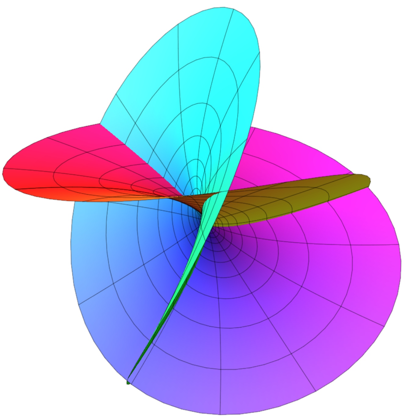
(a) $t=0$

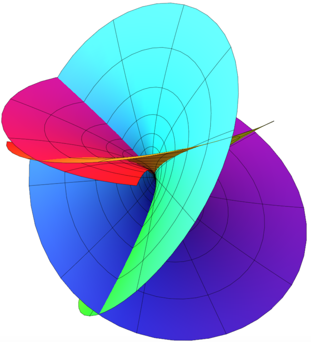
(b) $t=\frac{1}{4}$

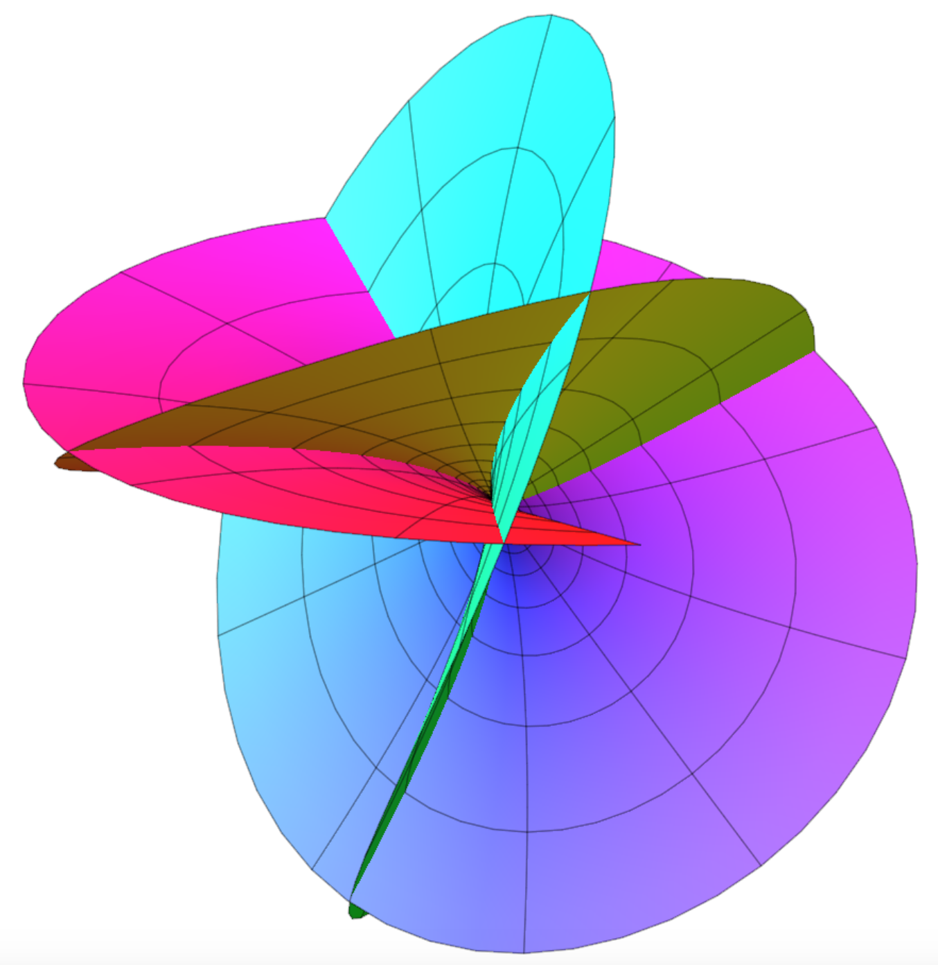
(c) $t=\frac{1}{2}$

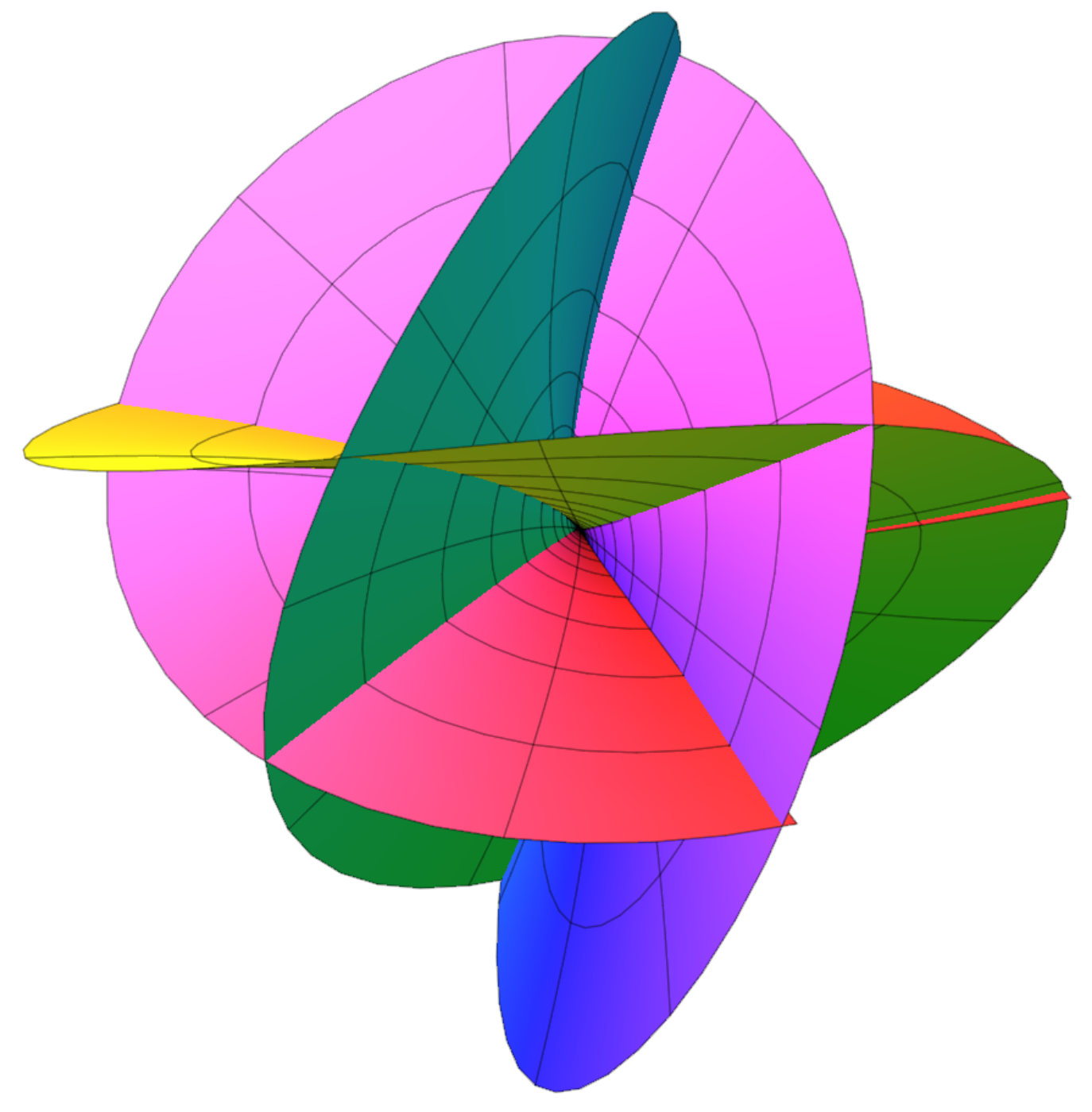
(d) $t=\frac{3}{4}$

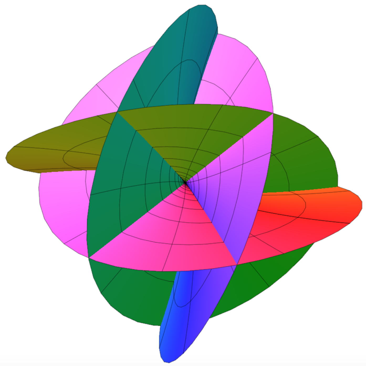
(e) $t=1$

Figure 2: Surfaces $\mathscr{S}_{t}$ extracted from the family described by the Weierstrass function $F_{t}$ in (78). They are images via the mapping $\bm{r}_{t}(w)$ induced by $F_{t}(w)$ through (54) of the disk $\mathbb{B}_{R}$ of radius $R$ centred at $w=0$; the scaling factor of each image is $|\bm{r}_{t}(R)|$.

As a supplement to this paper, we also provide an animation showing the whole family $\mathscr{S}_{t}$. We think that this makes it apparent how the moving surface progressively unfolds gliding over itself, with no sign of bending. In a companion animation, we also capture the motion that illustrates the classical association between catenoid and helicoid described by (71): it clearly conveys the same gliding impression.

We finally remark that by the change of variable $w\mapsto 1/w$ in (54) for $F=F_{\mathrm{B}}$ as in (79) Bour’s surfaces are shown to be invariant (to within a reflection) under the transformation $m\mapsto-m$. This makes catenoids and helicoids somehow special members of Bour’s family, as they are obtained from (79) for $m=0$.

V Conclusions

Understanding how surfaces deform is the proper foundation for a sound, intrinsic theory of plates and shells (as abundantly discussed, for example, in Sect. XIV.13 of [2]). Expressing the appropriate energy contents involved in the elasticity of these bodies requires a clear identification of the local independent modes for changing their shape.

Intuitively, we may say that there are only two such modes, that is, stretching and bending. Rigorously, we may associate unambiguously the former mode with the stretching component $\mathbf{U}$ of the surface deformation gradient $\mathbf{F}$, as delivered by the polar decomposition theorem. But associating the bending mode with the whole orthogonal component $\mathbf{R}$ of $\mathbf{F}$ cannot be right, as this deformation measure would in general fail to be intrinsic to the surface.

By decomposing uniquely $\mathbf{R}$ into a drilling rotation $\mathbf{R}^{\mathrm{(d)}}$ about the surface normal $\bm{\nu}$ and a complementary rotation $\mathbf{R}^{(\mathrm{b})}$ about an axis orthogonal to $\bm{\nu}$, we identified the latter as the correct bending measure. Bending-neutral deformations were then naturally defined as those deformations that would leave the bending content unchanged, while affecting the drilling one. In a variational elastic theory for shells, these deformations, if existent, would not affect the bending energy, while still prompting effective changes in shape, at the expenses of a drilling energy.

Whether bending-neutral deformations do actually exist is not a trivial issue. In this paper, we gave a necessary and sufficient integrability condition that guarantees their existence, al least locally. A large class of surfaces can indeed be subjected to bending-neutral deformations: all minimal surfaces. Actually, there is more to it: (1) every minimal surface is transformed into a minimal surface by a bending-neutral deformation and (2) given two generic minimal surfaces, there is a bending-neutral deformation mapping one into the other.

This implies that all minimal surfaces have a universal bending content.

All conceivable motions driving a minimal surface into another are such that drilling and stretching components of the deformation decomposition are the only ones responsible, as is apparent from the gliding motions shown in the animations accompanying this paper.

In the light of our finer decomposition of surface deformations, speaking of “a bending procedure which, at every stage, passes through a minimal surface” [34, p. 102], as done in almost every textbook, would be inaccurate: there is indeed no way to bend a minimal surface leaving it minimal; you can only drill it.

Although we deem our kinematic analysis of surfaces possibly also relevant to the energetics of elastic plates and shells, we have not attempted any systematic treatment of this issue. We are also guilty of another omission. Our deformation study was local in nature: we left out all global considerations. This came with the price of allowing self-intersecting surfaces as deformed images, which is forbidden in continuum mechanics by the principle of identification of material body points.

Appendix A Rotation Decomposition

Here we use equation (20) for the decomposition of a rotation $\mathbf{R}(\bm{a})\in\mathsf{SO}(3)$ to prove that the vectors $\bm{a}_{1}$ and $\bm{a}_{2}$ can be identified uniquely by requiring the former to be parallel to a given unit vector $\bm{e}$ and the latter orthogonal to it.

Let $\bm{a}\in\mathscr{V}$ and $\bm{e}\in\mathbb{S}^{2}$ be given so that $\bm{a}\times\bm{e}\neq\bm{0}$. We solve (21) with $\bm{a}_{1}=u\bm{e}$ and $\bm{a}_{2}\cdot\bm{e}=0$. Projecting both sides of (21) along $\bm{e}$ and on the plane orthogonal to it, we find that

$$u =\bm{a}\cdot\bm{e},$$ (80a)

$$\mathbf{P}(\bm{e})\bm{a} =\bm{a}_{2}-u\bm{e}\times\bm{a}_{2}.$$ (80b)

Representing $\bm{a}_{2}$ as

$$\bm{a}_{2}=b_{1}\mathbf{P}(\bm{e})\bm{a}+b_{2}\bm{e}\times\mathbf{P}(\bm{e})\bm{a},$$ (81)

where $b_{1}$ anb $b_{2}$ are scalar parameters to be determined, we easily see that the only solution of (80b) is obtained for

$$b_{1}=\frac{1}{1+u^{2}}\quad\text{and}\quad b_{2}=\frac{u}{1+u^{2}}.$$ (82)

Use of (82) and (80a) in (81) readily leads us to (22) in the main text.

To prove that $\mathbf{R}(\bm{a}_{1})$ with $\bm{a}_{1}$ as in (22) is indeed the rotation of $\mathsf{SO}(\bm{e})$ closest to $\mathbf{R}(\bm{a})$, we introduce the (squared) distance

$$d(u):=|\mathbf{R}(\bm{a})-\mathbf{R}(u\bm{e})|^{2}:=\operatorname{tr}\{[\mathbf{R}(\bm{a})-\mathbf{R}(u\bm{e})]^{\mathsf{T}}[\mathbf{R}(\bm{a})-\mathbf{R}(u\bm{e})]\}.$$ (83)

A direct computation shows that

$$d(u)=6+\frac{2}{1+a^{2}}\frac{1}{1+u^{2}}\{[1+a^{2}-4(\bm{a}\cdot\bm{e})^{2}]u^{2}-8(\bm{a}\cdot\bm{e})u+a^{2}-3\}$$ (84)

and it is then a simple matter to conclude that $d$ attains its minimum for $u=\bm{a}\cdot\bm{e}$ and its maximum for $u=-1/\bm{a}\cdot\bm{e}$.

Appendix B Gradient Integrability

In this appendix we gather a number of details needed to derive the integrability conditions in (41). The objective is to enforce (9) for the surface tensor field $\mathbf{F}=\mathbf{R}_{\bm{\nu}}(\alpha)\mathbf{U}_{\bm{y}}$ where $\mathbf{U}_{\bm{y}}$ is given by (37) and $\mathbf{R}_{\bm{\nu}}(\alpha)$ by (34).

We begin by writing $\mathbf{F}$ explicitly in the eigenframe $(\bm{n}_{1},\bm{n}_{2},\bm{\nu})$ of the curvature tensor,

$$\mathbf{F}=\lambda\{\kappa_{1}\cos\alpha\bm{n}_{1}\otimes\bm{n}_{1}+\kappa_{2}\sin\alpha\bm{n}_{1}\otimes\bm{n}_{2}+\kappa_{1}\sin\alpha\bm{n}_{2}\otimes\bm{n}_{1}-\kappa_{2}\cos\alpha\bm{n}_{2}\otimes\bm{n}_{2}\}.$$ (85)

To compute $\nabla\!_{\mathrm{s}}\mathbf{F}$, we also need to express both $\nabla\!_{\mathrm{s}}\bm{n}_{1}$ and $\nabla\!_{\mathrm{s}}\bm{n}_{2}$ in the frame $(\bm{n}_{1},\bm{n}_{2},\bm{\nu})$,

$$\begin{cases}\nabla\!_{\mathrm{s}}\bm{n}_{1}=\bm{n}_{2}\otimes\bm{c}-\kappa_{1}\bm{\nu}\otimes\bm{n}_{1},\\ \nabla\!_{\mathrm{s}}\bm{n}_{2}=-\bm{n}_{1}\otimes\bm{c}-\kappa_{2}\bm{\nu}\otimes\bm{n}_{2},\end{cases}$$ (86)

where $\bm{c}$ is the tangential field defined by (42).

A lengthy but simple calculation shows that equation (9) acquires the following structure

$$\bm{n}_{1}\otimes\mathbf{W}_{1}+\bm{n}_{2}\otimes\mathbf{W}_{2}=\bm{0},$$ (87)

where both $\mathbf{W}_{1}$ and $\mathbf{W}_{2}$ are skew-symmetric second-rank tensors, which by (85), (86), and (33) are associated with the following axial vectors

$$\begin{cases}\bm{w}_{1}=\nabla\!_{\mathrm{s}}(\lambda\kappa_{1}\cos\alpha)\times\bm{n}_{1}+\nabla\!_{\mathrm{s}}(\lambda\kappa_{2}\sin\alpha)\times\bm{n}_{2}-\lambda(\kappa_{1}+\kappa_{2})\mathbf{R}_{\bm{\nu}}(\alpha)\bm{n}_{2}\times\bm{c},\\ \bm{w}_{2}=\nabla\!_{\mathrm{s}}(\lambda\kappa_{1}\sin\alpha)\times\bm{n}_{1}-\nabla\!_{\mathrm{s}}(\lambda\kappa_{2}\cos\alpha)\times\bm{n}_{2}-\lambda(\kappa_{1}+\kappa_{2})\mathbf{R}_{\bm{\nu}}(\alpha)\bm{n}_{1}\times\bm{c},\end{cases}$$ (88)

which are both parallel to $\bm{\nu}$. The system of scalar equations (41) in the main text follows from requiring that $\bm{w}_{1}=\bm{w}_{2}\equiv\bm{0}$ on $\mathscr{S}$.

References

• Hildebrandt and Tromba [1996] S. Hildebrandt and A. Tromba, The Parsimonious Universe. Shape and Form in the Natural World (Springer-Verlag, New York, 1996).
• Antman [1995] S. S. Antman, Nonlinear Problems of Elasticity, Applied Mathematical Sciences, Vol. 107 (Springer, New York, 1995).
• Ghiba et al. [2020] I.-D. Ghiba, M. Bîrsan, P. Lewintan, and P. Neff, The isotropic Cosserat shell model including terms up to ${O}(h^{5})$. Part I: Derivation in matrix notation, J. Elast. 142, 201 (2020).
• Ghiba et al. [2021] I.-D. Ghiba, M. Bîrsan, P. Lewintan, and P. Neff, A constrained Cosserat shell model up to order ${O}(h^{5})$: Modelling, existence of minimizers, relations to classical shell models and scaling invariance of the bending tensor, J. Elast. 76, 83 (2021).
• Vitral and Hanna [2023a] E. Vitral and J. A. Hanna, Dilation-invariant bending of elastic plates, and broken symmetry in shells, J. Elast. 153, 571 (2023a).
• Vitral and Hanna [2023b] E. Vitral and J. A. Hanna, Energies for elastic plates and shells from quadratic-stretch elasticity, J. Elast. 153, 581 (2023b).
• Virga [2024] E. G. Virga, Pure measures of bending for soft plates, Soft Matter 20, 144 (2024).
• Acharya [2024] A. Acharya, Mid-surface scaling invariance of some bending strain measures, J. Elast. , 5517 (2024).
• Ghiba et al. [2023] I.-D. Ghiba, P. Lewintan, A. Sky, and P. Neff, An essay on deformation measures in isotropic thin shell theories. bending versus curvature (2023), arXiv:2312.10928 [math-ph] .
• Vitral and Hanna [2024] E. Vitral and J. A. Hanna, Assorted remarks on bending measures and energies for plates and shells, and their invariance properties (2024), arXiv:2405.06638 [cond-mat.soft] .
• Weatherburn [2016a] C. E. Weatherburn, Differential Geometry of Three Dimensions, Vol. I (Cambridge University Press, Cambridge, 2016).
• Šilhavý [2021] M. Šilhavý, A new approach to curvature measures in linear shell theories, Math. Mech. Solids 26, 1241 (2021).
• Kralj et al. [2011] S. Kralj, R. Rosso, and E. G. Virga, Curvature control of valence on nematic shells, Soft Matter 7, 670 (2011).
• Rosso et al. [2012] R. Rosso, E. G. Virga, and S. Kralj, Parallel transport and defects on nematic shells, Continuum Mech. Thermodyn. 24, 643 (2012).
• Weatherburn [2016b] C. E. Weatherburn, Differential Geometry of Three Dimensions, Vol. II (Cambridge University Press, Cambridge, 2016).
• Beltrami [1902] E. Beltrami, Opere Matematiche, Vol. 1 (Hoepli, Milan, 1902) available from https://gallica.bnf.fr/ark:/12148/bpt6k99432q/f1.item.
• Gurtin et al. [2010] M. E. Gurtin, E. Fried, and L. Anand, The Mechanics and Thermodynamics of Continua (Cambridge University Press, Cambridge, 2010).
• Man and Cohen [1986] C.-S. Man and H. Cohen, A coordinate-free approach to the kinematics of membranes, J. Elast. 16, 97 (1986).
• Gurtin and Murdoch [1975a] M. E. Gurtin and A. I. Murdoch, A continuum theory of elastic material surfaces, Arch. Rational Mech. Anal. 57, 291 (1975a), see also [42].
• Pietraszkiewicz et al. [2008] W. Pietraszkiewicz, M. Szwabowicz, and C. Vallée, Determination of the midsurface of a deformed shell from prescribed surface strains and bendings via the polar decomposition, Int. J. Non-Linear Mech. 43, 579 (2008).
• Palais et al. [2009] B. Palais, R. Palais, and S. Rodi, A disorienting look at Euler’s theorem on the axis of a rotation, Am. Math. Mon. 116, 892 (2009).
• Hughes and Brezzi [1989] T. J. Hughes and F. Brezzi, On drilling degrees of freedom, Comput. Methods Appl. Mech. Engrg. 72, 105 (1989).
• Fox and Simo [1992] D. Fox and J. Simo, A drill rotation formulation for geometrically exact shells, Comput. Methods Appl. Mech. Engrg. 98, 329 (1992).
• Mohammadi Saem et al. [2021] M. Mohammadi Saem, P. Lewintan, and P. Neff, On in-plane drill rotations for cosserat surfaces, Proc. R. Soc. Lond. A 477, 20210158 (2021).
• Altmann [1989] S. L. Altmann, Hamilton, Rodrigues, and the quaternion scandal, Math. Mag. 62, 291 (1989).
• Rodrigues [1840] O. Rodrigues, Des lois géométriques qui régissent les déplacements d’un système solide dans l’espace, et de la variation des coordonnées provenant de ces déplacements considérés indépendamment des causes qui peuvent les produire, J. Math. Pures Appl. 5, 380 (1840), available from http://www.numdam.org/item/JMPA_1840_1_5__380_0/.
• Mladenova and Mladenov [2011] C. D. Mladenova and I. M. Mladenov, Vector decomposition of finite rotations, Rep. Math. Phys. 68, 107 (2011).
• Martins and Podio-Guidugli [1979] L. C. Martins and P. Podio-Guidugli, A variational approach to the polar decomposition theorem, Atti Accad. Naz. Lincei Cl. Sci. Fis. Mat. Natur. Rend. 66, 487 (1979), available from http://www.bdim.eu/item?id=RLINA_1979_8_66_6_487_0.
• Martins and Podio-Guidugli [1980] L. C. Martins and P. Podio-Guidugli, An elementary proof of the polar decomposition theorem, Amer. Math. Month. 87, 288 (1980).
• Grioli [1940] G. Grioli, Una proprietà di minimo nella cinematica delle deformazioni finite, Boll. Un. Math. Ital. 2, 252 (1940), available from https://www.uni-due.de//imperia/md/content/mathematik/ag_neff/grioli_deformatione.pdf.
• Neff et al. [2014] P. Neff, J. Lankeit, and A. Madeo, On Grioli’s minimum property and its relation to Cauchy’s polar decomposition, Int. J. Eng. Sci. 80, 209 (2014).
• Ozenda et al. [2020] O. Ozenda, A. M. Sonnet, and E. G. Virga, A blend of stretching and bending in nematic polymer networks, Soft Matter 16, 8877 (2020).
• Ozenda and Virga [2021] O. Ozenda and E. G. Virga, On the Kirchhoff-Love hypothesis (revised and vindicated), J. Elast. 143, 359 (2021).
• Dierkes et al. [2010] U. Dierkes, S. Hildebrandt, and F. Sauvigny, Minimal Surfaces, 2nd ed., A Series of Comprehensive Studies in Mathematics, Vol. 339 (Springer, Berlin, 2010).
• Chern [1955] S.-S. Chern, An elementary proof of the existence of isothermal parameters on a surface, Proc. Amer. Math. Soc. 6, 771 (1955).
• Osserman [1986] R. Osserman, A Survey of Minimal Surfaces (Dover, Mineola, NY, 1986).
• Spivak [1999] M. Spivak, A Comprehensive Introduction to Differential Geometry, 3rd ed., Vol. 4 (Publish or Perish, Houston,Texas, 1999).
• Weierstrass [1903] K. Weierstrass, Untersuchungen über die Flächen, deren mittlere Krümmung überall gleich Null ist, in Mathematische Werke: Herausgegeben unter Mitwirkung einer von der königlich preussischen Akademie der Wissenschaften eingesetzten Commission, edited by J. Knoblauch (Mayer & Müller, Berlin, 1903) pp. 39–52, available from https://archive.org/details/mathematischewer03weieuoft/page/38/mode/2up.
• Weierstrass [2013] K. Weierstrass, Untersuchungen über die Flächen, deren mittlere Krümmung überall gleich Null ist, in Mathematische Werke: Herausgegeben unter Mitwirkung einer von der königlich preussischen Akademie der Wissenschaften eingesetzten Commission, Cambridge Library Collection – Mathematics, edited by J. Knoblauch (Cambridge University Press, Cambridge, 2013) pp. 39–52.
• Bour [1862] E. Bour, Théorie de la déformation des surfaces, J. Éc. Impériale Polytech. 39, 1 (1862).
• Cogliati and Rivis [2022] A. Cogliati and R. Rivis, The origins of the fundamental theorem of surface theory, Hist. Math. 61, 45 (2022).
• Gurtin and Murdoch [1975b] M. E. Gurtin and A. I. Murdoch, Addenda to our paper A continuum theory of elastic material surfaces, Arch. Rational Mech. Anal. 59, 389 (1975b).