Multi-Player Approaches for Dueling Bandits

Abstract

Various approaches have emerged for multi-armed bandits in distributed systems. The multiplayer dueling bandit problem, common in scenarios with only preference-based information like human feedback, introduces challenges related to controlling collaborative exploration of non-informative arm pairs, but has received little attention. To fill this gap, we demonstrate that the direct use of a Follow Your Leader black-box approach matches the lower bound for this setting when utilizing known dueling bandit algorithms as a foundation. Additionally, we analyze a message-passing fully distributed approach with a novel Condorcet-winner recommendation protocol, resulting in expedited exploration in many cases. Our experimental comparisons reveal that our multiplayer algorithms surpass single-player benchmark algorithms, underscoring their efficacy in addressing the nuanced challenges of the multiplayer dueling bandit setting.

1 Introduction

In decision-making under uncertainty, multi-armed bandit (MAB) [4] problems are a key paradigm with applications in recommendation systems and online advertising. These problems entail balancing exploration-exploitation trade-offs, as an agent draws from a set of $K$ arms with unknown reward distributions to maximize cumulative rewards or minimize regret over time. Two notable variations of MAB include the dueling-bandit problem and the cooperative multiplayer MAB problem. In the dueling-bandit scenario [36], feedback comes from pairwise comparisons between $K$ arms, useful in situations like human-feedback driven tasks, including ranker evaluation [25] and preference-based recommendation systems [10]. Meanwhile, the cooperative multiplayer MAB focuses on a group of $M$ players collaboratively solving challenges in a distributed decision-making environment, enhancing learning through shared information. This approach finds applications in fields like multi-robot systems [19] and distributed recommender systems [27].

The $M$-player $K$-arm cooperative dueling bandit problem, combining aspects of the two previously studied variations, introduces a new dimension to cooperative decision-making with preference-based feedback, yet remains unexplored to the best of our knowledge. A compelling application arises in large-scale distributed recommendation or ranker evaluation systems [12], where a network of backend servers directs users to local algorithms that elicit preference-based feedback. These systems, driven by high demand and the need for quick decisions, optimize performance through low-rate local communication with nearby servers, mirroring the dynamics of a multiplayer dueling bandit. Another example is a network of self-ordering machines in regional fast-food chains, where each machine collects customer preferences for food products [3]. Local communication is beneficial due to varied preferences across different areas.

The multiplayer dueling bandit setting, unlike its MAB counterpart, demands complex coordination for exploration-exploitation across pairs of arms. In multiplayer MAB, communication delays can lead to drawing suboptimal arms, but these still provide useful information that reduces future regret. In contrast, in multiplayer dueling bandits, communication delays can lead to pulling pairs of either identical or non-identical suboptimal arms. This not only results in immediate regret but also provides no new information in the former case, and limited information in the latter compared to pulling a pair of optimal and suboptimal arms. Thus, careful a communication strategy is crucial in this setting.

In this study, our focus centers on the widely explored Condorcet Winner (CW) assumption, in which there exists a unique preferable arm [32]. We establish an asymptotic regret lower bound of $O\left(K\log T\right)$ that is independent of player counts. We introduce a Follow Your Leader (FYL) black-box algorithm, that aligns well with existing dueling-bandit algorithms like Relative Upper Confidence Bound (RUCB) [40] and Relative Minimal Empirical Divergence (RMED) [16], and offers a more natural fit than multiplayer MAB variants [20]. Recognizing the limitations of relying solely on one leader for exploration [35], we also propose a decentralized extension to RUCB. Unlike in a MAB counterpart [11], we demonstrate that incorporating an additional CW recommendation protocol between players significantly accelerates the identification of the CW in many instances. We validate our approach with real-world data experiments. To summarize, our contributions encompass:

• We propose an intuitive black-box algorithm adept at integrating with existing single-player dueling bandit algorithms, conduct comprehensive regret analysis, and illustrate its capability to match an established lower bound when initialized with the RMED algorithm.

• We conduct an in-depth regret analysis of a fully decentralized multiplayer algorithm based on RUCB, showcasing asymptotic optimality of the incurred regret up to constants.

• We demonstrate that a novel CW recommendation protocol results in a quick identification of the CW in many instances.

• Through simulated experiments on real data, we substantiate our claim that our algorithms exhibit superior performance compared to a single-player dueling bandit system.

The remainder of this paper is structured as follows: Section 2 introduces the problem and articulates a regret lower bound. Section 3 proposes the black box algorithm. In Section 4, we analyze a fully distributed algorithm. Section 5 showcases experimental results, and Section 6 concludes the paper.

Related Work

The dueling bandit problem, introduced as a useful variant of the MAB problem in Yue & Yoachims [37], initially underwent analysis with stringent assumptions about the preference matrix. These assumptions, including stochastic transitivity and stochastic triangle inequality, resulted in regret bounds of $O(K\log T)$ [38, 36]. Subsequent works relaxed these assumptions by introducing the more realistic CW assumption [40, 16, 9, 1], which remains widely adopted today. Notably, the RUCB algorithm [40], based on the UCB approach for MAB, achieves an $O(K\log T)$ regret with high probability. Komiyama et al. [16] established a comprehensive lower bound for this setting of the same order and provided the RMED family of algorithms that match it. Recently, Saha & Gaillard [29] demonstrated a general reduction from dueling bandit algorithms to MAB and introduced a best-of-both-worlds algorithm effective for both adversarial and stochastic dueling bandits. Other recent advancements include a batched variant [2] and a differentially private extension [28]. Additionally, in cases where the CW does not exist, alternative definitions of winners, such as the Borda Winner [13] and the Copeland Winner [17, 39], have been considered in dueling bandit literature.

Considerable attention utilizing various approaches has been directed towards cooperative multiplayer MAB scenarios, revealing an $O(K\log T)$ regret lower bound [11]. Among them, in an approach called the leader-follower paradigm, players designate one or multiple leaders and base their arm selections on the leaders’ instructions. In Kolla et al. [15] and Landgren et al. [20], followers emulate leaders employing a UCB strategy with neighbor-only communication, but the resulting algorithm does not match the lower bound. In the context of a Bernoulli bandit, Wang et al. [33] introduced a distributed parsimonious exploration strategy with message passing akin to ours called DPE2, in which a leader explores using a UCB strategy, and followers exploit a designated arm sent by it. Their approach showcased a regret that aligns with the lower bound, but required a meticulous derivation that cannot be applied in general. In the fully distributed setting, which is more suitable in situations where players are non-synchronized or should have similar performance, both a message-passing approach [11, 23] and a running-consensus approach [21] yield a regret that matches the lower bound up to constants. Alternatively, certain approaches adopt a gossiping strategy [8, 30], in which a player can randomly communicate with one other player at each round.

2 Problem Formulation

For some matrix $W$, $w_{ij}$ will denote the $(i,j)$-th element. In the $M$-player $K$-arm dueling bandit problem, each player $m\in[M]=\{1,2,\ldots,M\}$ engages in the environment at each round by drawing an arm pair $\left(i_{m}(t),j_{m}(t)\right)\in[K]^{2}$ and receiving a Bernoulli reward feedback $r_{i_{m}(t),j_{m}(t)}=1-r_{j_{m}(t),i_{m}(t)}$, where $\mathbb{E}r_{i_{m}(t),j_{m}(t)}=q_{i_{m}(t),j_{m}(t)}$ for preference matrix $Q\in\mathbb{R}^{K\times K}$. $Q$ is a symmetric matrix unknown to players that satisfies $q_{ii}=0.5$ for all $i\in[K]$. For brevity, we will use $r_{m}(t)$ when the context is clear. In this work, we assume that there exists a Condorcet Winner (CW), which is an arm $i$ such that $q_{ij}>0.5$ for all $i\neq j$, and without loss of generality assume that the CW is arm $1$. We further denote by $\mathcal{Q}_{\mathrm{CW}}$ the class of preference matrices with a CW.

Players are positioned on a connected undirected communication graph $\mathcal{G}=\left(\mathcal{V},\mathcal{E}\right)$, where $\mathcal{V}=[M]$ denotes the vertices and $\mathcal{E}$ represents the set of edges. We denote $d(m,m^{\prime})$ as the length of the shortest path between players $m,m^{\prime}$ on $\mathcal{G}$, and $D=\max_{m,m^{\prime}}d(m,m^{\prime})$ as the diameter of the graph. Additionally, the $\gamma$-power of $\mathcal{G}$ for a positive integer $\gamma$, denoted $\mathcal{G}_{\gamma}$, is a graph that shares $\mathcal{G}$’s vertices but includes an edge between any two vertices within a distance of $\gamma$ or less in $\mathcal{G}$. The clique covering number of $\mathcal{G}$ is the minimum number of cliques required to include every vertex. Communication operates under a message-passing protocol [11, 23] with a decay parameter $\gamma$. Each round, player $m$ sends a message $x_{m}^{m^{\prime}}(t)$ to each player $m^{\prime}$, which is received after $d(m,m^{\prime})-1$ rounds if $\gamma>d(m,m^{\prime})-1$ or is otherwise never obtained. This extends the traditional models of immediate reward sharing where only immediate neighbors communicate ($\gamma=1$) [15], and delayed communication in which all players communicate with each other under delays ($\gamma=D$) [7].

The number of wins of arm $i$ over arm $j$ experienced by player $m$ until round $t$ is $w_{ij}^{m}(t)=\sum_{\tau=1}^{t}\left(r_{m}(\tau)\mathds{1}\{(i_{m}(\tau),j_{m}(\tau))=(i,j)\}+(1-r_{m})(\tau)\mathds{1}\{(i_{m}(\tau),j_{m}(\tau))=(j,i)\}\right)$. Additionally, $N_{ij}^{m}(t)=\sum_{\tau=1}^{t}(w_{ij}^{m}(\tau)+w_{ji}^{m}(\tau))$ represents the number of visits to $(i,j)$ or $(j,i)$. We denote $\Delta_{ij}=q_{ij}-1/2$ as the reward gap, and define the cumulative regret as $\mathcal{R}(T)=\sum_{m=1}^{M}\sum_{t=1}^{T}0.5(\Delta_{1i_{m}(t)}+\Delta_{1j_{m}(t)})$. Note that the instantaneous regret for a given player is zero only if the player draws the CW twice in a given round. Additionally, we define $\Delta_{1\max}:=\max\{\Delta_{1i}\}$ and $\Delta_{1\min}:=\min_{i>1}\{\Delta_{1i}\}$.

Asymptotic Lower Bound

We first establish a lower bound for the multiplayer dueling bandit setting in Theorem 2.1 Let $\mathcal{O}_{i}=\{j|j\in[K],q_{ij}<1/2\}$ denote the superiors of arm $i$. An algorithm is considered consistent over the class $\mathcal{Q}_{\mathrm{CW}}$ if $\mathbb{E}\mathcal{R}(T)=o(T^{p})$ for all $p>0$ and $Q\in\mathcal{Q}_{\mathrm{CW}}$. Furthermore, we define $N_{ij}(T)=\sum_{m=1}^{M}N_{ij}^{m}(T)$ as the total number of visits to $(i,j)$ or $(j,i)$ in the system, and $\mathrm{KL}(p,q)=p\log\frac{p}{q}+(1-p)\frac{1-p}{1-q}$ as the Kullback-Leibler (KL) divergence between Bernoulli distributions.

Theorem 2.1.

For any consistent algorithm on $\mathcal{Q}_{\mathrm{CW}}$ and $Q\in\mathcal{Q}_{\mathrm{CW}}$, the group regret obeys:

$$\liminf_{T\rightarrow\infty}\frac{\mathbb{E}\mathcal{R}(T)}{\log T}\geq\sum_{i\in[K]\setminus\{1\}}\min_{j\in\mathcal{O}_{i}}\frac{\Delta_{1i}+\Delta_{1j}}{2\mathrm{KL}(q_{ij},1/2)}.$$

This bound scales as $O(K\log T)$ similarly to the single-player case [16], irrespective of the number of players $M$. This is straightforward from the fact that a multiplayer system cannot perform better than in a centralized setting consisting of a single player that draws $M$ pairs at each round. Nevertheless, in Appendix A, we prove Theorem 2.1 in a novel way compared to the single-player setting. To do so, we first leverage a carefully constructed divergence decomposition in Lemma A.8. We then derive a challenging environment instance, which is more difficult compared to the MAB setting [22] due to the structured nature of the problem, and employ information-theoretic bounds in Lemma A.9. These bounds are more useful in the multiplayer case compared to existing single-player techniques [16], which are more cumbersome and less applicable in this setting.

3 Follow Your Leader Black Box Algorithm

We now present our first main contribution: a Follow Your Leader multiplayer algorithm capable of employing a single-player base dueling bandit algorithm as a black box. We begin with the following assumption regarding the base algorithm.

1 Input: Time horizon $T$, number of arms $K$, number of players $M$, communication graph $\mathcal{G}=(\mathcal{V},\mathcal{E})$, Base algorithm Alg0, Leader Election algorithm LEAlg, Election time $T_{\mathrm{LE}}$.

2 Initialize: $i(m)=1$ for $m\in\mathcal{V}$.

3 for $t=1,\ldots,T_{\mathrm{LE}}$ do

4       Each player communicates with neighbors according to LEAlg.

5       Each player draws arms $(c(t),d(t))$ according to Alg0.

6      

7

8for $t=T_{\mathrm{LE}}+1,\ldots,T$ do

9       Leader $m_{l}$:

10       Draw arms $(c(t),d(t))$ according to Alg0.

11       Get CW candidate $\mathrm{cw}(t)$ from Alg0.

12       if $\mathrm{cw}(t-1)\neq\mathrm{cw}(t)$ then

13             Send $\mathrm{cw}(t)$ over the communication graph.

14            

15      

16      Followers:

17       for $m\in[M]\setminus\{m_{l}\}$ do

18             if new arm $i$ arrives from leader then

19                   $i(m)\leftarrow i$.

20                  

21            Draw pair $(i(m),i(m))$.

22            

23      

Algorithm 1 Follow Your Leader Black Box (FYLBB)

Assumption 3.1.

Given a single-player history up to time $t$, the base algorithm outputs:

1. A pair of arms $(c(t),d(t))$ to draw.

2. A CW candidate $\mathrm{cw}(t)$, such that $\mathbb{E}\left[\sum_{t=1}^{T}\mathds{1}\{\mathrm{cw}(t)\neq 1\}\right]\leq f(K,T,Q)~{}.$

Furthermore, it has a regret upper bound of $\mathbb{E}\mathcal{R}(T)\leq g(K,T,Q)$, where $f,g$ denote some functions, and $f=o(g)$ with respect to $T$.

The algorithm starts with a distributed leader-election phase, utilizing some algorithm LEAlg. This is a well-studied problem with a range of efficient algorithms available [31, 18], typically requiring minimal communication. For simplicity, we concentrate on deterministically identified leader election, where each player is assumed to be initialized with a unique integer identifier and communicates integer values [6]. This algorithm classifies each player as either “leader” or “non-leader”, with only one player holding the former designation, and is completed in $T_{\mathrm{LE}}$ time steps, independent of $T$. An illustrative example of such an algorithm can be found in Appendix B. During this initial phase, all players independently draw arms based on the base algorithm. For rounds $t=T_{\mathrm{LE}}+1,\ldots,T$, the elected leader $m_{l}$ continues to draw arms similarly without receiving feedback from other players, and in rounds where $\mathrm{cw}(t-1)\neq\mathrm{cw}(t)$, initiates a message containing the new $\mathrm{cw}(t)$. This is facilitated through a message-passing protocol with a decay parameter equivalent to the diameter of the communication graph. Simultaneously, each follower $m$ engages in pure exploitation by drawing the arm pair $(i(m),i(m))$, where $i(m)$ is the arm last received from the leader.

While our setup resembles the DPE2 algorithm for multiplayer MAB [33] introduced in Section Related Work, Algorithm 1 works with any base algorithm, unlike DPE2 which utilizes a specific exploration strategy that requires a meticulous derivation. In addition, unique to the dueling-bandit setting, followers are restricted to pure exploitation of the form $(\mathrm{cw}(t),\mathrm{cw}(t))$, meaning they gain no information about the preference matrix. Thanks to this property, it is relatively easy to adapt single-player dueling bandit algorithms to this framework by presenting a candidate arm $\mathrm{cw}(t)$, which is typically a crucial element in the original algorithm. Consequently, our algorithm achieves broader applicability.

Theorem 3.2.

Under Assumption 3.1, Algorithm 1 satisfies:

$$\mathbb{E}\mathcal{R}(T)\leq g(K,T,Q)+M\Delta_{1\max}f(K,T,Q)+M(T_{\mathrm{LE}}+2D)\Delta_{1\max}~{}.$$

Additionally, the expected number of communication rounds is bounded by $T_{\mathrm{LE}}+2f(K,T,Q)$, where a communication round is defined as a round in which some player initiates communication.

Theorem 3.2 demonstrates that, in the asymptotic regime, the regret of Follow Your Leader Black Box (FYLBB) is dominated by the single-player regret bound $g$, thus inheriting the same asymptotic performance. Another encouraging result is that communication is not initiated at each round and is bounded by $f$, which is often sublogarithmic in $T$. The proof involves decomposing the group regret resulting from the leader election phase, the leader itself, followers’ exploitation rounds when $i(m)$ is not the CW, and communication rounds where a message from the leader has yet to reach followers. We establish that all these components are bounded by $f$ and $g$ in a corresponding single-player setting with the base algorithm, which enables us to prove a regret bound despite the generality of this setting. The detailed proof is available in Appendix B.

This construction enables us to seamlessly adapt single-player dueling bandit results to multiplayer scenarios and even attain asymptotically optimal algorithms without the need for difficult reconstructions, as demonstrated next.

Corollary 3.3.

For any $\epsilon>0$ and $\alpha>1$, the following holds for the regret bound of Algorithm 1.

1. For RUCB [40] as the base algorithm:

   $$\mathbb{E}\mathcal{R}(T) =\sum_{i=2}^{K}\frac{4\alpha\log T}{\Delta_{1i}}+O\left(MD+M\frac{K^{2}\log K}{\Delta^{2}_{1\min}}\right)~{}.$$

2. For RMED2FH [16] as the base algorithm:

   $$\mathbb{E}\mathcal{R}(T) =\sum_{i=2}^{K}\min_{j\in\mathcal{O}_{i}}\frac{\Delta_{1i}+\Delta_{1j}}{2\mathrm{KL}(q_{ij},1/2)}+O\left(MD+MK^{2+\epsilon}\log\log T+\frac{K\log T}{\log\log T}\right)~{}.$$

By employing RMED2FH as the base algorithm, our approach achieves performance that aligns with the lower bound outlined in Theorem 2.1 in the asymptotic regime. Utilizing RUCB yields an $O(K\log T)$ algorithm that remains independent of $M$ under these conditions. Notably, for both algorithms, the candidate $\mathrm{cw}(t)$ corresponds to an arm already retained by the original algorithms.

While Algorithm 1 is versatile and can leverage any base algorithm satisfying Assumption 3.1 with comparable asymptotic guarantees, its empirical performance is suboptimal in certain scenarios, as demonstrated in Section 5. This arises from the lack of cooperation for exploration, as indicated by the term $O\left(Mf(K,T,Q)\right)$, representing the regret incurred by the leader in identifying the CW. Moreover, an FYLBB approach is less suitable for systems where players enter and exit dynamically. These concerns motivate us to develop an expedited exploration approach in the next section.

4 A Fully Distributed Approach

While Algorithm 1 offers an intuitive black-box approach, exploration without cooperation can lead to significant finite-time regret, motivating us to introduce a distributed strategy in this section. We demonstrate that a novel message-passing extension of RUCB in Algorithm 2 where players share rewards and update the CW candidate based on recommendations from other players, is an effective distributed approach for this setting. Unlike a naive message-passing extension [23] which would modify the RUCB algorithm such that data sent by other players is only utilized to construct improved confidence intervals, in Algorithm 2 CW candidates are also shared between players. This fosters a more effective exploration and adds a layer of complexity to the network interactions, thereby complicating the analysis of regret bounds. Detailed proofs for the claims in this section are found in Appendix C.

In lines 5–21 of Algorithm 2, each player follows a local version of RUCB.

1 Input: Time horizon $T$, number of arms $K$, number of players $M$, $\alpha>1.2$, communication graph $\mathcal{G}=(\mathcal{V},\mathcal{E})$, decay parameter $\gamma$.

2 Initialize: $\tilde{W}^{m}:=(\tilde{w}_{ij}^{m}),\tilde{N}^{m}:=(\tilde{N}_{ij}^{m})\leftarrow 0_{K\times K},\mathcal{B}^{m},\mathcal{B}^{m}_{\mathrm{rec}},x_{m}(t)\leftarrow\emptyset,~{}$ $\forall~{}t\leq 1,~{}m\in\mathcal{V}$.

3 for $t=1,2,\ldots,T$ do

4       for $m=1,\ldots,M$ do

             $U^{m}:=(u_{ij}^{m})\leftarrow\frac{\tilde{W}^{m}}{\tilde{N}^{m}}+\sqrt{\frac{\alpha\log t}{\tilde{N}^{m}}}$.

              // Elementwise, $x/0:=1$.

5             $u_{ii}^{m}\leftarrow 0.5$ for $i\in[K]$.

6             $\mathcal{C}^{m}\leftarrow\{i\mid u_{ij}^{m}\geq 0.5\ \forall j\in[K]\}$.

7             $\mathcal{B}^{m}\leftarrow\mathcal{B}^{m}\cap\mathcal{C}^{m}$.

8             If $|\mathcal{C}^{m}|=1$ then $\mathcal{B}^{m}\leftarrow\mathcal{C}^{m}$.

9             If $|\mathcal{B}^{m}_{\mathrm{rec}}\cap\mathcal{C}^{m}|\geq 1$ then set $\mathcal{B}^{m}$ to a random element from $\mathcal{B}^{m}_{\mathrm{rec}}\cap\mathcal{C}^{m}$.

10             if $\mathcal{C}^{m}=\emptyset$ then

11                   pick $i_{m}(t)$ randomly from $[K]$.

12                  

13             else

14                   if $\mathcal{B}^{m}\cap\mathcal{C}^{m}\neq\emptyset$ then

15                         pick $i_{m}(t)$ from $\mathcal{B}^{m}$.

16                        

17                   else

18                         pick $i_{m}(t)$ randomly from $\mathcal{C}^{m}$.

19                        

20                  

            $j_{m}(t)\leftarrow\operatorname*{argmax}_{j}u_{ji}^{m}$.

              // If tie $i_{m}(t)\neq j_{m}(t)$.

21             Draw $(i_{m}(t),j_{m}(t))$ and obtain $r_{m}(t)$.

22             $x_{m}(t)\leftarrow\langle m,t,i_{m}(t),j_{m}(t),r_{m}(t)\rangle$.

23             Send $x_{m}(t)$ in message-passing.

24            

25      for $m=1,\ldots,M$ do

26             $x^{m}(t)\leftarrow\{x_{m^{\prime}}(t^{\prime})\mid d(m,m^{\prime})=t-t^{\prime}\leq\gamma-1\}$.

27             Update $\tilde{W}^{m}$ with samples in $x^{m}(t)$.

28             $\tilde{N}^{m}\leftarrow\tilde{W}^{m}+(\tilde{W}^{m})^{T}$.

29             $\mathcal{B}^{m}_{\mathrm{rec}}\leftarrow\{i\mid(i,i)\in x_{m^{\prime}}(t^{\prime})\land d(m,m^{\prime})=t-t^{\prime}\leq\gamma-1\}$.

30            

31      

32

Algorithm 2 Message-Passing RUCB (MP-RUCB)

To compute the UCB terms $u_{ij}^{m}$ for each arm pair $(i,j)$, player $m$ maintains the matrix $\tilde{W}^{m}(t):=(\tilde{w}^{m}_{ij}(t))$. Here, $\tilde{w}^{m}_{ij}(t)$ represents information about the number of wins of $i$ against $j$ up to round $t$, known to the player from their own and other players’ experiences up to that round. Similarly, $\tilde{N}^{m}(t):=(\tilde{N}^{m}_{ij}(t))$ represents the known number of visits up to round $t$. This is distinct from the local counters $w^{m}_{ij}(t)$ and $N_{ij}^{m}(t)$, which results in each player utilizing information gathered by other players in their decision-making. Additionally, each player maintains its own champion set $\mathcal{C}^{m}$ with arms likely to win against all other arms, a CW candidate set $\mathcal{B}^{m}$ that may either contain one candidate arm or be empty, and a set of recommended arms $\mathcal{B}^{m}_{\mathrm{rec}}$. The CW candidate set $\mathcal{B}^{m}$ is updated with a random element from $\mathcal{C}^{m}\cap\mathcal{B}^{m}_{\mathrm{rec}}$ whenever this set is non-empty, and is otherwise updated based on $\mathcal{C}^{m}$. Players communicate through a message-passing protocol with a decay parameter $\gamma$, as described in Section 2. For simplicity, we denote the message sent by player $m$ at round $t$ as $x_{m}(t)$ in line 22, which contains the drawn arms and the sampled reward. In lines 26–29, players receive messages and update $\tilde{W}^{m}$ and $\tilde{N}^{m}$ based on their own arms and reward samples, as well as those received from other players. Moreover, whenever a new message includes an exploitation draw of the same arm twice, that arm is added to the recommended set $\mathcal{B}^{m}_{\mathrm{rec}}$ for use in the next round.

We begin with a lemma that shows with high probability that for rounds larger than

$$C(\delta):=\left(4MK^{2}\left(3+2\log\left(d_{\max}^{\gamma}+1\right)\right)/\delta\right)^{\frac{1}{1.7\alpha-1.4}}~{},$$

visitation numbers to arm pairs other than $(1,1)$ cannot be too large across the system.

Lemma 4.1.

For any $\alpha>1.2$, $\delta>0$ and $T_{0}\geq C(\delta)$, define $N_{ij}^{m,T_{0}}(t)$ as the number of visitations of player $m$ to $(i,j)$ between rounds $T_{0}$ and $t$, and $\overline{\Delta}_{ij}:=\min\{\Delta_{1i},\Delta_{1j}\}$ for $i,j\neq 1$, $\overline{\Delta}_{1i}:=\Delta_{1i}$. Additionally, for some $\gamma^{\prime}\leq\gamma$ let $\mathcal{C}(\mathcal{G}_{\gamma^{\prime}})$ be the set of all cliques in $\mathcal{G}_{\gamma^{\prime}}$. Then, with probability larger than $1-\delta$, rounds $t>T_{0}$, parameters $\gamma^{\prime}\leq\gamma$, cliques $C\in\mathcal{C}(\mathcal{G}_{\gamma^{\prime}})$ and pairs $(i,j)\neq(1,1)$ such that $\sum_{m\in C}N_{ij}^{m,T_{0}}(t)>\left[4\alpha\log t/\overline{\Delta}_{ij}^{2}+(\gamma^{\prime}+2)|C|\right]\mathds{1}\{i\neq j\}$ do not exist.

The establishment of this bound is pivotal, as it allows us to both bound the leading term of the group regret with a multiplicative factor smaller than $M$, and to bound the non-leading term in $T$ corresponding to the regret incurred before identifying the CW. A naive analysis akin to the single-player case would lead to only bounding the local counters $N_{ij}^{m,T_{0}}(t)$, resulting in a regret that scales like $O(MK\log T)$. To avoid that, we capitalize on the shared observations among players to limit the total number of visits within any clique, and rely on the fact that the first arm is drawn from the player-specific champion set regardless of recommendations. Unlike existing multiplayer MAB methods [23], we demonstrate the visitation counter bound holds with high probability even for rounds in which the pair $(i,j)$ is not drawn by any player, and for any clique in the graph to facilitate faster CW identification.

Before presenting the group regret bound for Algorithm 2, we introduce the following term.

$$\tilde{C}=\frac{1.7\alpha-2.4}{1.7\alpha-1.4}\left(4MK^{2}\left(3+2\log\left(d_{\max}^{\gamma}+1\right)\right)\right)^{\frac{1}{1.7\alpha-1.4}}.$$

Theorem 4.2.

For any $\delta>0$ and $\gamma^{\prime}\leq\gamma$, define $\mathcal{D}:=\sum_{i<j}4\alpha/\overline{\Delta}_{ij}^{2}$, $\Gamma(m,\gamma^{\prime})$ as the size of the largest clique player $m$ belongs to in $\mathcal{G}_{\gamma^{\prime}}$ and

$$\hat{C}: =\Delta_{1\max}\sum_{m=1}^{M}\min_{\gamma^{\prime}\leq\gamma}\left(K^{2}(\gamma^{\prime}+2)+\frac{2\mathcal{D}}{\Gamma(m,\gamma^{\prime})}\log 2\mathcal{D}\right)+(2\tilde{C}+K(3\gamma+2))M\Delta_{1\max}~{}.$$

Let $\chi(\mathcal{G}_{\gamma})$ denote the clique covering number of $\mathcal{G}_{\gamma}$. Then for any $\alpha>1.4$ and all times $T$:

$$\mathbb{E}\mathcal{R}(T) \leq\sum_{j>1}\frac{2\alpha\chi(\mathcal{G}_{\gamma})}{\Delta_{1j}}\log T+\hat{C}~{}.$$

The regret bound presented in Theorem 4.2 demonstrates that a message-passing protocol is an effective distributed approach for the dueling bandit problem. It emphasizes the significance of leveraging candidate recommendations in reducing the regret incurred before identifying the CW, a characteristic unique to this scenario. In the asymptotic regime, the regret scales as $O\left(K\chi(\mathcal{G}_{\gamma})\log T\right)$, consistent with distributed approaches in the multiplayer MAB setting [11, 23]. For the no communication case ($\gamma=0$), this translates to an $O\left(MK\log T\right)$ bound, while for complete communication ($\gamma=D$), where every player can communicate with any other, the regret scales optimally as $O\left(K\log T\right)$.

Similarly, in the finite-time regime, the non-dominant term $\hat{C}$ is non-increasing with $\gamma$, and is determined separately for each graph $\mathcal{G}$ and parameter $\gamma$ by minimization over two competing delay-dependent terms. While providing a direct expression for this term is difficult, in a complete communication setting it scales like $O\left(MKD+\frac{K^{2}\log K}{\Delta^{2}_{1\min}}+MK^{2}\min\Big{\{}\frac{\log K}{\Delta^{2}_{1\min}},D\Big{\}}\right)$ as discussed in Appendix C, and we observe a tradeoff between the delay $D$ and the instance complexity $1/\Delta^{2}_{1\min}$. For challenging instances where $\Delta^{2}_{1\min}$ is sufficiently small, the non-leading term scales as $O(K^{2}\log K/\Delta^{2}_{1\min})$ compared to the $O(MK^{2}\log K/\Delta^{2}_{1\min})$ term for Follow Your Leader RUCB (FYLRUCB). This observation helps explain the better empirical performance observed in Section 5.

Proving Theorem 4.2 is a challenging task, necessitating the establishment that each player actively identifies the CW quicker than a single-player counterpart and that visitation counters within cliques cannot be too large with high probability. To achieve this, we leverage Lemma 4.1 and demonstrate that, owing to CW candidate recommendations, each player identifies the CW within $O\left(\gamma+K^{2}\gamma^{\prime}+K^{2}\log(K)/\Gamma(m,\gamma^{\prime})\Delta^{2}_{1\min}\right)$ rounds with high probability for any clique such that $\gamma^{\prime}\leq\gamma$. We then decompose the regret to accommodate both the finite-time and asymptotic regimes. In the latter, each player consistently selects the CW as the first arm, leading to a high probability regret bound that is later converted into an expected regret bound using basic probability properties.

5 Experiments

In this section, we present experimental results to assess the empirical performance of Algorithms 1 and 2. The simulations were conducted using three preference matrices:

Six rankers: Consists of 6 arms and is based on the six retrieval functions used in the engine of ArXiv.org [38].
Sushi: Derived from the Sushi preference dataset [14], which contains preference data from 5000 users over 100 types of Sushi. We use a 10-kinds dataset [24] and convert it into a preference matrix, where $q_{ij}$ denotes the ratio of users who prefer kind $i$ over $j$.
Irish election: Based on the 2002 Dublin Meath election dataset [26], encompassing 64,081 votes over 14 candidates. We extracted the 10 most preferred candidates and constructed a preference matrix similarly to the Sushi dataset. This dataset was also employed in recent works [1].

The proposed datasets all feature a CW. We conduct a comparison between Algorithm 1 with both RMED2FH and RUCB as base algorithms, alongside Algorithm 2. Additional experimental results and details can be found in Appendix D.

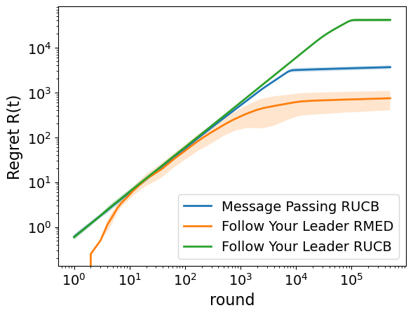
(a) Six Rankers

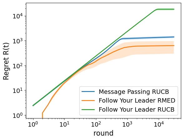
(b) Sushi

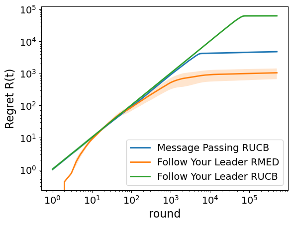
(c) Irish

Figure 1: Group regret for all datasets, using a complete communication graph with 10 players.

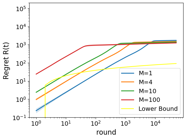
(a) Message Passing RUCB

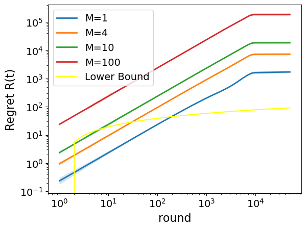
(b) Follow Your Leader RUCB

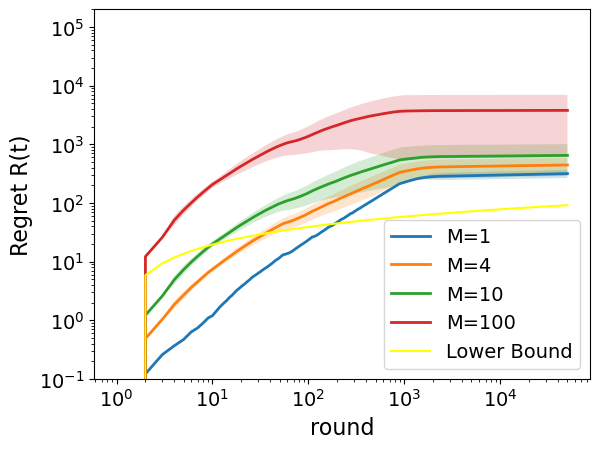
(c) Follow Your Leader RMED

Figure 2: Group regret for the Sushi dataset: A complete graph with a varying number of players.

Algorithmic Comparisons Across Datasets

We first present a comparative analysis of the three algorithms across all four datasets, as depicted in Figure 1. The group regret per round is illustrated on a log-log scale, considering a scenario where players are situated on a complete graph with $M=10$ nodes. Across all datasets, we observe both the finite-time regime, dominated by exploration, and the asymptotic one, where the CW has been captured. In each dataset, FYLRMED consistently outperforms the other algorithms, while FYLRUCB exhibits the least favorable performance. As previously mentioned, in these algorithms, exploration is predominantly executed by the leader.

The superior performance of FYLRMED can be attributed to the enhanced exploration-exploitation tradeoff achieved by RMED2FH compared to RUCB, emphasizing that the overall performance of FYLBB is greatly influenced by the choice of the base algorithm. Message-passing RUCB showcases the significance of cooperation during exploration, leading to the early discovery of the CW compared to FYLRUCB, as indicated by the earlier transition into the asymptotic regime. Consequently, we have substantially lower regret when compared to the latter, despite both employing a similar decision-making process.

Experiments with a Varying Number of Players

In Figure 2, we depict the group regret using the Sushi dataset and all algorithms, on a complete communication graph with a varying number of players $M=1,4,10,100$, along with the lower bound. The results illustrate that, as anticipated by the regret bounds, the regret in the asymptotic regime remains unaffected by the number of players $M$. Notably, RMED2FH is the sole algorithm aligning with the lower bound. In contrast to the two other algorithms, Message-Passing RUCB rapidly identifies the CW as the number of players increases. This leads to enhanced group performance, supporting the results outlined in Section 4.

Comparisons with a Single Player

In Figure 3, we show the average regret per player in a 10-player group for each algorithm. Additionally, we include the regret of a single player and the regret of a single player capable of making 10 actions in each round, divided by 10. We utilize the Sushi dataset and use a complete communication graph for the multiplayer setting. Notably, for all algorithms, a single player with only one action per round exhibits inferior performance in the asymptotic regime.

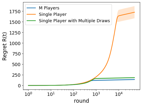
(a) Message Passing RUCB

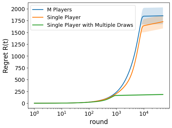
(b) Follow Your Leader RUCB

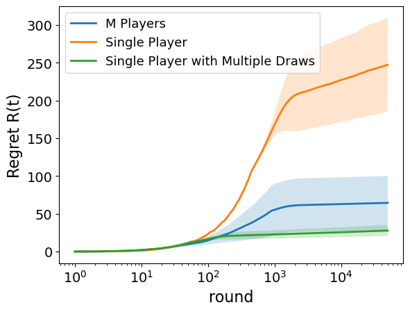
(c) Follow Your Leader RMED

Figure 3: Average regret for the Sushi dataset with $M=10$ players: a 10-player group, a single player, and a single player with 10 draws in each round.

This observation underscores the evident advantage of employing multiplayer systems. Conversely, a single player with 10 actions per round simulates a centralized 10-player system, where decision-making by a central entity benefits from all available information. Across all algorithms, the average player in a multiplayer system exhibits a comparable slope in the asymptotic regime to that of the average player in a centralized system, emphasizing their similar performance. This reaffirms that, asymptotically, our algorithms successfully emulate the behavior of a centralized system.

Comparisons Across Different Graph Structures

Figure 4 depicts the group regret per round for the Sushi dataset and all algorithms, employing complete, cycle, star and path communication graphs with 100 players. For FYLBB algorithms, the leader is the central node in the star graph.

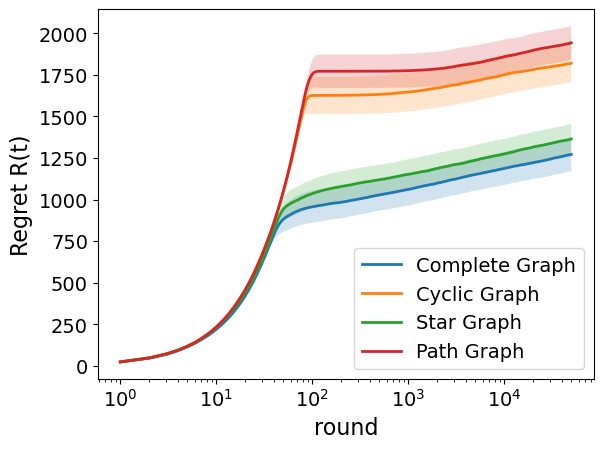
(a) Message Passing RUCB

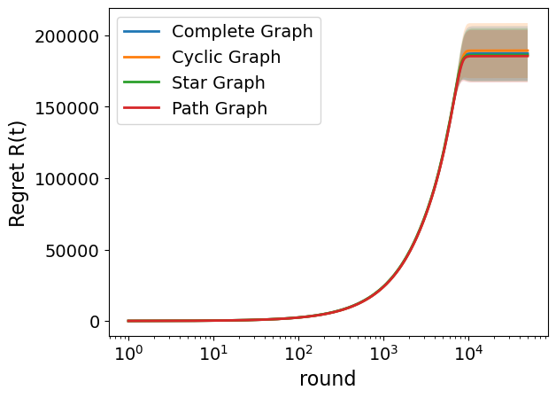
(b) Follow Your Leader RUCB

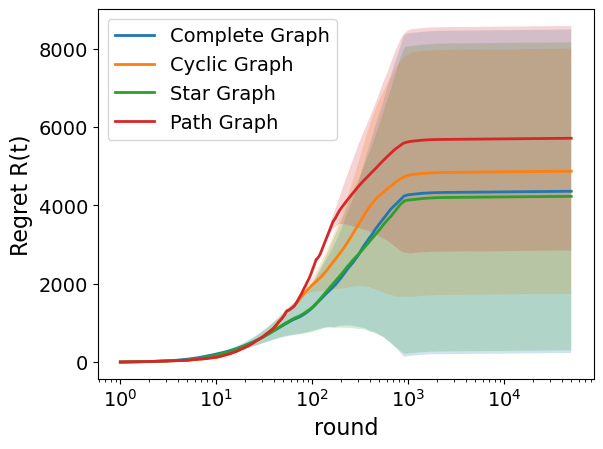
(c) Follow Your Leader RMED

Figure 4: Group regret for the Sushi dataset: different communication graphs with $M=100$ players.

Alternatively, it is the outermost node in the path graph. Notably, for Message Passing RUCB a complete graph and a star graph, with diameters of $1$ and $2$ respectively, outperform a cycle graph with a diameter of $50$ and a path graph with a diameter of $99$, due to delayed CW identification, as discussed in Section 4. This distinction is less apparent in the case of FYLBB algorithms, where the capture of the CW occurs later on average and dominates the incurred regret.

6 Conclusion and Future Work

This paper introduced novel approaches to address the multiplayer dueling bandit problem, demonstrating the existence of efficient algorithms despite the increased complexity compared to a MAB setting. We established a regret lower bound for this problem and discussed a versatile black-box algorithm, leveraging either RUCB or RMED as base algorithms. However, as demonstrated in the experimental evaluation, finite-time performance can vary depending on the exploration efficiency of the base algorithm. To address this, we devised a novel message-passing protocol with CW recommendations for RUCB, showcasing more consistent performance and quick identification of the CW. All algorithms exhibited asymptotic regret comparable to that of a single player, a result validated theoretically and through simulations.

In future work, one promising avenue is the development of a black-box algorithm capable of compatibility with diverse base algorithms, while also enhancing collaborative exploration. A parallel approach could involve devising a multiplayer black-box algorithm using a base multiplayer bandit algorithm. Additionally, making our algorithms more practical for real-world applications could involve incorporating federated learning [34] and privacy-preserving methods [5].

Appendix A Lower Bound Proof

This section consists of two subsections. In Section A.1, we establish a precise definition for a canonical probability space tailored to the multiplayer dueling bandit scenario. Following this foundational definition, Section A.2 presents a comprehensive proof for the lower bound encapsulated in Theorem 2.1. To ensure clarity and coherence, we revisit key definitions introduced in Section 2.

A.1 A Canonical Probability Space

Definition A.1.

A stochastic dueling bandit environment is a collection of distributions $\nu=\left(P_{ij}:i,j\in[K]\right)$, where $K$ is the number of available actions, and $P_{ij}$ is a Bernoulli distribution with mean $q_{ij}$, such that $q_{ij}=1-q_{ji}$.

In this context, the preference matrix $Q=(q_{ij})\in\mathbb{R}^{K\times K}$ represents a given environment. Next, we define a class of preference matrices.

Definition A.2.

A dueling bandit environment class is $\mathcal{Q}=(Q)$ is some collection of preference matrices. In particular, we define

1. The class of preference matrices with total ordering: $\mathcal{Q}_{\mathrm{o}}=\{Q~{}|~{}i\prec j\Leftrightarrow q_{ij}<1/2\}$.

2. The class of preference matrices with a Condorcet Winner (CW): $\mathcal{Q}_{\mathrm{CW}}=\{Q~{}|~{}\exists i:q_{ij}>1/2~{}\forall j\neq i\}$.

Note that $\mathcal{Q}_{\mathrm{o}}\subset\mathcal{Q}_{\mathrm{CW}}$. Now, let $T$ be the time horizon. We consider $M$ players communicating via a connected, undirected graph $\mathcal{G}=(\mathcal{V},\mathcal{E})$. Communication is bidirectional, and any message sent from player $m$ may be obtained by player $m^{\prime}$ after $d(m,m^{\prime})-1$ rounds of the bandit problem, where $d(m,m^{\prime})$ denotes the length of the shortest path between players $m$ and $m^{\prime}$ on $\mathcal{G}$. Let $(i_{m}(t),j_{m}(t))$ denote the pair drawn by player $m$ at time $t$, and $r_{m}(t)$ denote the corresponding reward. The power graph of order $\gamma$ of $\mathcal{G}$, denoted by $\mathcal{G}_{\gamma}$, is defined to include an edge $(m,m^{\prime})$ if there exists a path of length at most $\gamma$ in $\mathcal{G}$ between players $m$ and $m^{\prime}$. the neighborhood of $m$ in $\mathcal{G}_{\gamma}$ is given by $\mathcal{N}_{\gamma}(m)$, including player $m$ itself. We establish a communication protocol as follows.

Assumption A.3.

Players can communicate in the following manner:

• Any player $m$ is capable of sending a message $x_{m}^{m^{\prime}}(t)$ to any other player $m^{\prime}\in\mathcal{N}_{\gamma}(m)$ at time $t$, and this message may be received by player $m^{\prime}$ at time $t+\min(0,d(m,m^{\prime})-1)$. This is done via a message-passing protocol as described in Section 2

• The message $x_{m}^{m^{\prime}}(t)$ is a function of the arms-reward triplets of player $m$ up to and including time $t$, i.e. $x_{m}^{m^{\prime}}(t)=F_{m,t}^{m^{\prime}}\left(i_{m}(1),j_{m}(1),r_{m}(1),\ldots,i_{m}(t),j_{m}(t),r_{m}(t)\right)$ for any deterministic Borel function $F_{m,t}^{m^{\prime}}:\mathbb{R}^{3t}\rightarrow\mathbb{R}^{L}$, with $L$ being a nonnegative integer.

To define a measurable probability space for this setting, let us treat the players as ordered, such that player $1$ is the first one and player $M$ is the last. We define the outcome until time $t$ and player $m$ as the ordered set $H_{m,t}=(i_{1}(1),j_{1}(1),r_{1}(1),\ldots,i_{m}(t),j_{m}(t),r_{m}(t))$, the outcome space as $\Omega_{m,t}=([K]^{2}\times\mathbb{R})^{M(t-1)+mt}$, and the corresponding sigma-algebra as $\mathcal{F}_{m,t}=\mathcal{B}(\Omega_{m,t})$. Here, $\mathcal{B}(\cdot)$ stands for the Borel sigma-algebra. Using these, we define a measurable space for the entire multiplayer dueling bandit problem as $\left(\Omega_{M,T},\mathcal{F}_{M,T}\right)$, with the random variables of the drawn arms and obtained rewards as

$$i_{m}(t)\left(i_{1,1},j_{1,1},x_{1,1},\ldots,i_{M,T},j_{M,T},r_{M,T}\right) =i_{m,t}~{},$$

$$j_{m}(t)\left(i_{1,1},j_{1,1},x_{1,1},\ldots,i_{M,T},j_{M,T},r_{M,T}\right) =j_{m,t}~{},$$

$$r_{m}(t)\left(i_{1,1},j_{1,1},x_{1,1},\ldots,i_{M,T},j_{M,T},r_{M,T}\right) =r_{m,t}.$$

For clerity, we also define the player-specific measurable space as $\left(\Omega_{T}^{m},\mathcal{F}_{T}^{m}\right)$, where $H_{t}^{m}=(i_{m}(1),j_{m}(1),r_{m}(1),\ldots,i_{m}(t),j_{m}(t),r_{m}(t))$, $\Omega_{t}^{m}=\left([K]^{2}\times\mathbb{R}\right)^{t}$, and $\mathcal{F}_{t}^{m}=\mathcal{B}(\Omega_{t}^{m})$. Next, we define the multiplayer dueling bandit policy, which can be separated into a communication policy and an action policy. This separation is motivated by the fact that both aspects are under the control of the learner.

Definition A.4.

A communication policy $\tilde{\Pi}_{\mathrm{comm},\gamma}$ for the multiplayer dueling bandit setup is the sequence of messages $(F_{m,t}^{m^{\prime}})_{m,m^{\prime},t}$ from Assumption A.3, where $m\in[M],t\in[T]$ and $m^{\prime}\in\mathcal{N}_{\gamma}(m)~{}\forall m\in[M]$.

Definition A.5.

An action policy $\tilde{\Pi}$ for the multiplayer dueling bandit setup is a sequence $(\tilde{\Pi}_{t})_{t=1}^{T}$ where $\tilde{\Pi}_{t}=(\tilde{\Pi}_{t}^{m})$, and $\tilde{\Pi}_{t}^{m}$ is a probability kernel from $\left(\Omega_{t-1}^{m}\times\mathbb{R}^{L_{m,t}^{\gamma}},\mathcal{B}\left(\Omega_{t-1}^{m}\times\mathbb{R}^{L_{m,t}^{\gamma}}\right)\right)$ to $([K]^{2},2^{[K]^{2}})$, where $L_{m,t}^{\gamma}=L\sum_{m^{\prime}\in\mathcal{N}_{\gamma}(m)\backslash\{m\}}(t-d(m,m^{\prime}))$. We define $\tilde{\pi}_{t}=(\tilde{\pi}_{t}^{m})$ as the corresponding density with respect to the counting measure on $([K]^{2},2^{[K]^{2}})$, so that $\forall i,j\in[K]$

$$\tilde{\pi}_{t}^{m}\left(i,j|h_{t-1}^{m},z_{t}^{m}\right)=\tilde{\Pi}_{t}^{m}\left(\{i,j\}|h_{t-1}^{m},z_{t}^{m}\right).$$

Here, where $z_{t}^{m}$ stands for all the messages received by player $m$ until round $t$.

The communication policy $\tilde{\Pi}_{\mathrm{comm},\gamma}$ and the action policy $\tilde{\Pi}$ as defined above illustrate the nature through which a learner operates, are easy to extract from an algorithm, and will help define the probability density function of the outcome. However, we can combine them into a more convenient policy definition that only takes into account the outcomes in $\Omega_{M,T}$.

Definition A.6.

A policy $\Pi$ for the multiplayer dueling bandit setup is a sequence $(\Pi_{t})_{t=1}^{T}$ where $\Pi_{t}=(\Pi_{t}^{m})$, and $\Pi_{t}^{m}$ is a probability kernel from $\left(\Omega_{t-1}^{m}\times\prod_{m^{\prime}\in\mathcal{N}_{\gamma}(m)\backslash\{m\}}\Omega_{t-d(m,m^{\prime})}^{m^{\prime}},\mathcal{B}\left(\Omega_{t-1}^{m}\times\prod_{m^{\prime}\in\mathcal{N}_{\gamma}(m)\backslash\{m\}}\Omega_{t-d(m,m^{\prime})}^{m^{\prime}}\right)\right)$ to $([K]^{2},2^{[K]^{2}})$. We define $\pi_{t}=(\pi_{t}^{m})$ as the corresponding density with respect to the counting measure on $([K]^{2},2^{[K]^{2}})$, so that $\forall i,j\in[K]$

$$\pi_{t}^{m}\left(i,j\Bigg{|}h_{t-1}^{m}\times\prod_{m^{\prime}\in\mathcal{N}_{\gamma}(m)\backslash\{m\}}h_{t-d(m,m^{\prime})}^{m^{\prime}}\right)=\tilde{\pi}_{t}^{m}\left(i,j|h_{t-1}^{m},z_{t}^{m}\right).$$

We are now ready to define the probability measure on $\left(\Omega_{M,T},\mathcal{F}_{M,T}\right)$, which can be done in two ways similar to the MAB setting [22]. As a first definition, we require that -

• The conditional distribution of $i_{m}(t),j_{m}(t)$ given $i_{1}(1),\ldots,r_{m-1}(t)$ (in case $m>1$, or $i_{1}(1),\ldots,r_{M}(t-1)$ otherwise) is $\Pi_{t}^{m}$ almost surely.

• The conditional distribution of $r_{m}(t)$ given $i_{1}(1),\ldots,r_{m-1}(t),i_{m}(t),j_{m}(t)$ is $P_{i_{m}(t),j_{m}(t)}(r_{m}(t))$ almost surely.

This defines a unique probability measure on $\left(\Omega_{M,T},\mathcal{F}_{M,T}\right)$. Alternatively, as a second definition, we can also define a probability measure with respect to a probability density function (pdf). Let $\lambda$ be a $\sigma$-finite measure on $(\mathbb{R},\mathcal{B}(\mathbb{R}))$ for which $P_{ij}$ is absolutely continuous with respect to $\lambda$ for all $i,j\in[K]$. denote $p_{ij}=dP_{ij}/d\lambda$, and let $\rho$ be the counting measure on $([K]^{2},2^{[K]^{2}})$ (since $P_{ij}$ is Bernoulli, we can take $\lambda$ to be the Lebesgue measure, so that $p_{ij}(x)=q_{ij}x+(1-q_{ij})x$). Utilizing Fubini’s theorem and the properties of the Radon-Nikodym derivative, the pdf of an outcome is

$$p_{\nu\pi}(i_{1,1},j_{1,1},r_{1,1},\ldots,i_{M,T},j_{M,T},r_{M,T})$$

$$=\prod_{t=1}^{T}\prod_{m=1}^{M}\pi_{t}^{m}\left(i_{m,t},j_{m,t}|h_{t-1}^{m}\times\prod_{m^{\prime}\in\mathcal{N}_{\gamma}(m)\backslash\{m\}}h_{t-d(m,m^{\prime})}^{m^{\prime}}\right)p_{i_{m,t},j_{m,t}}(r_{m,t}),$$

and the measure can be calculated as

$$\mathbb{P}_{\nu\pi}(B)= \int_{B}\left(p_{\nu\pi}(i_{1,1},j_{1,1},r_{1,1},\ldots,i_{M,T},j_{M,T},r_{M,T})(\rho\times\lambda)^{MT}\right.$$

$$\quad\left.\times d(i_{1,1},j_{1,1},r_{1,1},\ldots,i_{M,T},j_{M,T},r_{M,T})\right)~{}\forall B\in\mathcal{F}_{M,T}.$$

As mentioned before, these two definitions result in the same probability measure.

A.2 Proof for Theorem 2.1

First, we present a useful decomposition for the group regret within the context of multiplayer dueling bandits. Throughout this section, we will frequently employ the notation $\mathbb{E}\mathcal{R}_{\mathcal{G},T}(\pi,\nu)$ instead of $\mathbb{E}\mathcal{R}(T)$ to underscore its dependence on various terms.

$$\mathbb{E}\mathcal{R}_{\mathcal{G},T}(\pi,\nu) =\mathbb{E}_{\nu}\left[\sum_{t=1}^{T}\sum_{m=1}^{M}\frac{\Delta_{1i_{m}(t)}+\Delta_{1j_{m}(t)}}{2}\right]$$

$$=\frac{1}{2}\sum_{i\in[K]}\sum_{j\in[K]\setminus\{i\}}\frac{\Delta_{1i}+\Delta_{1j}}{2}\mathbb{E}_{\nu}N_{ij}(T)+\sum_{i\in[K]}\Delta_{1i}\mathbb{E}_{\nu}N_{ii}(T).$$

Here, the subscript $\nu$ signifies that the expectation is evaluated for bandit environment $\nu$. In adittion, $N_{ij}(T)=\sum_{t=1}^{T}\sum_{m=1}^{M}\left(\mathds{1}\{i_{m}(t)=i,j_{m}(t)=j\}+\mathds{1}\{i_{m}(t)=j,j_{m}(t)=i\}\right)$ for $i\neq j$ and $N_{ii}(T)=\sum_{t=1}^{T}\sum_{m=1}^{M}\mathds{1}\{i_{m}(t)=i,j_{m}(t)=i\}\}$ represent the total number of visits to arms $(i,j)$ by time $T$ without order. We proceed to define the class of consistent policies, a class for which the lower bound holds.

Definition A.7.

A policy $\pi$ for the multiplayer dueling bandit setup is called consistent over a class of bandits $\mathcal{Q}$ if for all $Q\in\mathcal{Q}$ and $p>0$, it holds that

$$\lim_{T\rightarrow\infty}\frac{\mathbb{E}\mathcal{R}_{\mathcal{G},T}(\pi,\nu)}{T^{p}}=0.$$

The class of consistent policies over $\mathcal{Q}$ is denoted by $\Pi_{\mathrm{cons}}(\mathcal{Q})$.

Next, we present a divergence decomposition lemma tailored to the multiplayer dueling bandit setting. This will be used to prove the lower bound.

Lemma A.8.

Let $\nu=(P_{ij})$ and $\nu^{\prime}=(P_{ij}^{{}^{\prime}})$ be two stochastic dueling bandit environments. Fix some multiplayer policy $\pi$ such that Assumption A.3 holds, and let $\mathbb{P}_{\nu\pi}$ and $\mathbb{P}_{\nu^{\prime}\pi}$ denote the probability measures for the canonical bandit models induced by the $T$-round interconnection of $\pi$ and $\nu,\nu^{\prime}$ respectively. Then,

$$\mathrm{KL}\left(\mathbb{P}_{\nu\pi},\mathbb{P}_{\nu^{\prime}\pi}\right)=\frac{1}{2}\sum_{i\in[K]}\sum_{j\in[K]\setminus\{i\}}\mathbb{E}_{\nu}[N_{ij}(T)]\mathrm{KL}(q_{ij},q_{ij}^{{}^{\prime}}),$$

where $\mathrm{KL}(\mathbb{P},\mathbb{Q})$ stands for the KL divergence between probability measures $\mathbb{P},\mathbb{Q}$

$$\mathrm{KL}\left(\mathbb{P},\mathbb{Q}\right)=\mathbb{E}_{\mathbb{P}}\left[\log\left(\frac{d\mathbb{P}}{d\mathbb{Q}}\right)\right],$$

and $\mathrm{KL}(p,q)$ stands for the KL divergence between two Bernoulli measures with means $p,q$ respectively.

Proof.

Assume that $\mathrm{KL}\left(q_{ij},q_{ij}^{{}^{\prime}}\right)<\infty$ for all $i,j\in[K]$. It follows from the KL-divergence definition that $P_{ij}\ll P_{ij}^{{}^{\prime}}$. Next, define the measure $\lambda=\sum_{i=1}^{K}(P_{ij}+P_{ij}^{{}^{\prime}})$ for which $P_{ij},P_{ij}^{{}^{\prime}}\ll\lambda$ for all $i,j\in[K]$.

It is evident that the policy terms $\pi_{t}^{m}$ remain consistent across bandit environments $\nu$ and bandit $\nu^{\prime}$ when our interest lies in the same outcome. This consistency arises from Assumption A.3, which ensures that messages are deterministic functions of the outcome and are otherwise independent of the environment. Additionally, a policy is uniquely determined by action-reward pairs and messages. Therefore, using the pdf of the outcome with respect to the product measure $(\rho\times\lambda)^{MT}$ for each environment:

$$\log\frac{d\mathbb{P}_{\nu\pi}}{d\mathbb{P}_{\nu^{\prime}\pi}}(i_{1,1},\ldots,r_{M,T})=\sum_{t=1}^{T}\sum_{m=1}^{M}\log\frac{p_{i_{m,t},j_{m,t}}(r_{m,t})}{p_{i_{m,t},j_{m,t}}^{{}^{\prime}}(r_{m,t})}~{},$$

and

$$\mathbb{E}_{\nu}\left[\log\frac{d\mathbb{P}_{\nu\pi}}{d\mathbb{P}_{\nu^{\prime}\pi}}(i_{1,1},\ldots,r_{M,T})\right]=\sum_{t=1}^{T}\sum_{m=1}^{M}\mathbb{E}_{\nu}\left[\log\frac{p_{i_{m,t},j_{m,t}}(r_{m,t})}{p_{i_{m,t},j_{m,t}}^{{}^{\prime}}(r_{m,t})}\right].$$

For every term in the sum we have that

$$\mathbb{E}_{\nu}\left[\log\frac{p_{i_{m,t},j_{m,t}}(r_{m,t})}{p_{i_{m,t},j_{m,t}}^{{}^{\prime}}(r_{m,t})}\right] =\mathbb{E}_{\nu}\left[\mathbb{E}_{\nu}\left[\log\frac{p_{i_{m,t},j_{m,t}}(r_{m,t})}{p_{i_{m,t},j_{m,t}}^{{}^{\prime}}(r_{m,t})}\Big{|}i_{m,t},j_{m,t}\right]\right]$$

$$=\mathbb{E}_{\nu}\left[\mathrm{KL}(P_{i_{m,t},j_{m,t}},P_{i_{m,t},j_{m,t}}^{{}^{\prime}})\right].$$

Returning to the previous equation:

$$\mathbb{E}_{\nu} \left[\log\frac{d\mathbb{P}_{\nu\pi}}{d\mathbb{P}_{\nu^{\prime}\pi}}(i_{1,1},\ldots,r_{M,T})\right]=\sum_{t=1}^{T}\sum_{m=1}^{M}\mathbb{E}_{\nu}\left[\mathrm{KL}(P_{i_{m,t},j_{m,t}},P_{i_{m,t},j_{m,t}}^{{}^{\prime}})\right]$$

$$=\sum_{i,j=1}^{K}\mathbb{E}_{\nu}\left[\sum_{t=1}^{T}\sum_{m=1}^{M}\mathds{1}\{(i_{m,t}=i,j_{m,t}=j)\}\mathrm{KL}(P_{ij},P_{ij}^{{}^{\prime}})\right]$$

$$=\frac{1}{2}\sum_{i\in[K]}\sum_{j\in[K]\setminus\{i\}}\mathbb{E}_{\nu}[N_{ij}(T)]\mathrm{KL}(P_{ij},P_{ij}^{{}^{\prime}})+\sum_{i\in[K]}\mathbb{E}_{\nu}[N_{ii}(T)]\mathrm{KL}(P_{ij},P_{ij}^{{}^{\prime}})$$

$$=\frac{1}{2}\sum_{i\in[K]}\sum_{j\in[K]\setminus\{i\}}\mathbb{E}_{\nu}[N_{ij}(T)]\mathrm{KL}(q_{ij},q_{ij}^{{}^{\prime}})+\sum_{i\in[K]}\mathbb{E}_{\nu}[N_{ii}(T)]\mathrm{KL}(q_{ii},q_{ii}^{{}^{\prime}})$$

$$=\frac{1}{2}\sum_{i\in[K]}\sum_{j\in[K]\setminus\{i\}}\mathbb{E}_{\nu}[N_{ij}(T)]\mathrm{KL}(q_{ij},q_{ij}^{{}^{\prime}}),$$

where in the last transition we used the fact that $q_{ii}=q_{ii}^{{}^{\prime}}=1/2$. Given that $d\mathbb{P}_{\nu\pi}/d\mathbb{P}_{\nu^{\prime}\pi}<\infty$, it holds that

$$\mathrm{KL}\left(\mathbb{P}_{\nu\pi},\mathbb{P}_{\nu^{\prime}\pi}\right)=\mathbb{E}_{\nu}\left[\log\frac{d\mathbb{P}_{\nu\pi}}{d\mathbb{P}_{\nu^{\prime}\pi}}\right].$$

It is evident that in our case the expectation is finite, so

$$\mathrm{KL}\left(\mathbb{P}_{\nu\pi},\mathbb{P}_{\nu^{\prime}\pi}\right)=\frac{1}{2}\sum_{i\in[K]}\sum_{j\in[K]\setminus\{i\}}\mathbb{E}_{\nu}[N_{ij}(T)]\mathrm{KL}(q_{ij},q_{ij}^{{}^{\prime}}).$$

In case $\mathrm{KL}(q_{ij},q_{ij}^{{}^{\prime}})=\infty$ for some $i,j\in[K]$, this relation still holds since both sides of the equation become infinite. ∎

We also use the following lemma.

Lemma A.9.

For any consistent algorithm on $\mathcal{Q}_{\mathrm{CW}}$ and $Q\in\mathcal{Q}_{\mathrm{CW}}$, and for any arm $i\in[K]\setminus\{1\}$ the following holds.

$$\liminf_{T\rightarrow\infty}\frac{\mathbb{E}\left[\sum_{j\in\mathcal{O}_{i}}\mathrm{KL}(q_{ij},1/2)N_{ij}(T)\right]}{\log T}\geq 1.$$

Proof.

Fix some arm $i\in[K]\setminus\{1\}$ and define $\mathcal{O}_{i}^{{}^{\prime}}=\{j~{}|~{}j\in[K],q_{ij}\leq 1/2\}$. We consider a challenging instance $Q^{{}^{\prime}}$, which is defined such that the means $q_{ij}^{{}^{\prime}}$ for $j\in\mathcal{O}_{i}^{{}^{\prime}}$ satisfy $\mathrm{KL}(q_{ij},q_{ij}^{{}^{\prime}})=\mathrm{KL}(q_{ij},1/2)+\epsilon$ with $q_{ij}^{{}^{\prime}}>1/2$, for some $\epsilon>0$ (we leave $q_{ii}^{{}^{\prime}}=q_{ii}=1/2$). The rest of the means remain the same as $q_{ij}$. For this new instance, $Q^{{}^{\prime}}\in\mathcal{Q}_{\mathrm{CW}}$ and arm $i$ is the CW.

It is important to highlight that a proof scheme akin to ours that is used for MAB [22] is applicable only to an unstructured class of bandits. This is due to the necessity of the unstructured assumption to construct the challenging instance $\nu^{{}^{\prime}}$. The unstructured assumption becomes crucial when attempting to change the mean of a single arm, as the presence of interdependence among arms restricts such modifications. In the dueling bandit scenario, we can directly provide a challenging instance within the structured class, even though the arms’ means may be correlated. This distinction allows for a more flexible approach to constructing challenging instances within the dueling bandit framework.

Note that since only the means $q_{ij}$ for $j\in\mathcal{O}_{i}^{{}^{\prime}}$ are different in the two environments, Lemma A.8 states that

$$\mathrm{KL}\left(\mathbb{P}_{\nu\pi},\mathbb{P}_{\nu^{\prime}\pi}\right)=\sum_{j\in\mathcal{O}_{i}^{{}^{\prime}}}\mathrm{KL}(q_{ij},q_{ij}^{{}^{\prime}})\mathbb{E}_{\nu}\left[N_{ij}(T)\right]\leq\sum_{j\in\mathcal{O}_{i}^{{}^{\prime}}}(\mathrm{KL}(q_{ij},1/2)+\epsilon)\mathbb{E}_{\nu}\left[N_{ij}(T)\right].$$

From the Bretagnolle-Huber inequality, for any event $A\in\mathcal{F}_{M,T}$,

$$\mathbb{P}_{\nu\pi}(A)+\mathbb{P}_{\nu^{\prime}\pi}(A^{c}) \geq\frac{1}{2}\exp\left(-\mathrm{KL}\left(\mathbb{P}_{\nu\pi},\mathbb{P}_{\nu^{\prime}\pi}\right)\right)$$

$$\geq\frac{1}{2}\exp\left(-\sum_{j\in\mathcal{O}_{i}^{{}^{\prime}}}(\mathrm{KL}(q_{ij},1/2)+\epsilon)\mathbb{E}_{\nu}\left[N_{ij}(T)\right]\right).$$

Choose $A=\{N_{ii}(T)>MT/2\}$, and let $\mathcal{R}_{\mathcal{G}}:=\mathcal{R}_{\mathcal{G},T}(\pi,\nu),\mathcal{R}_{\mathcal{G}}^{{}^{\prime}}:=\mathcal{R}_{\mathcal{G},T}(\pi,\nu^{\prime})$. By the Markov inequality

$$\mathcal{R}_{\mathcal{G}}\geq\Delta_{1i}\mathbb{E}_{\nu}\left[N_{ii}(T)\right]\geq\frac{MT\Delta_{1i}}{2}\mathbb{P}_{\nu\pi}\left(N_{ii}(T)\geq\frac{MT}{2}\right)=\frac{MT\Delta_{1i}}{2}\mathbb{P}_{\nu\pi}(A).$$

Additionally, the regret for the challenging instance is

$$\mathcal{R}_{\mathcal{G}}^{{}^{\prime}} =\frac{1}{2}\sum_{l\in[K]\setminus\{i\}}\sum_{j\in[K]\setminus\{i,l\}}\frac{\Delta_{il}^{{}^{\prime}}+\Delta_{ij}^{{}^{\prime}}}{2}\mathbb{E}_{\nu^{{}^{\prime}}}N_{lj}(T)$$

$$+\sum_{j\in[K]}\Delta_{ij}^{{}^{\prime}}\mathbb{E}_{\nu^{{}^{\prime}}}N_{jj}(T)+\sum_{j\in[K]\setminus\{i\}}\frac{\Delta_{ij}^{{}^{\prime}}}{2}\mathbb{E}_{\nu^{{}^{\prime}}}N_{ij}(T).$$

By definition, since arm $i$ is the CW for the challenging instance, the minimal gap with respect to it $\Delta_{min}^{{}^{\prime}}=\min_{j\in[K]\setminus\{i\}}\Delta_{ij}^{{}^{\prime}}$ is positive, so

$$\mathcal{R}_{\mathcal{G}}^{{}^{\prime}} \geq\frac{1}{2}\sum_{l\in[K]\setminus\{i\}}\sum_{j\in[K]\setminus\{i,l\}}\frac{\Delta_{min}^{{}^{\prime}}/2+\Delta_{min}^{{}^{\prime}}/2}{2}\mathbb{E}_{\nu^{{}^{\prime}}}N_{lj}(T)$$

$$+\sum_{j\in[K]\setminus\{i\}}(\Delta_{min}^{{}^{\prime}}/2)\mathbb{E}_{\nu^{{}^{\prime}}}N_{jj}(T)+\sum_{j\in[K]\setminus\{i\}}\frac{\Delta_{min}^{{}^{\prime}}}{2}\mathbb{E}_{\nu^{{}^{\prime}}}N_{ij}(T)$$

$$=\frac{\Delta_{min}^{{}^{\prime}}}{2}\mathbb{E}_{\nu^{{}^{\prime}}}\left[\frac{1}{2}\sum_{l\in[K]\setminus\{i\}}\sum_{j\in[K]\setminus\{i,l\}}N_{lj}(T)+\sum_{j\in[K]\setminus\{i\}}N_{jj}(T)+\sum_{j\in[K]\setminus\{i\}}N_{ij}(T)\right]$$

$$=\frac{\Delta_{min}^{{}^{\prime}}}{2}\mathbb{E}_{\nu^{{}^{\prime}}}\left[MT-N_{ii}(T)\right]\geq\frac{\Delta_{min}^{{}^{\prime}}}{2}(MT-\frac{MT}{2})\mathbb{P}_{\nu^{{}^{\prime}}\pi}\left(MT-N_{ii}(T)\geq MT-\frac{MT}{2}\right)$$

$$=\frac{MT\Delta_{min}^{{}^{\prime}}}{4}\mathbb{P}_{\nu^{{}^{\prime}}\pi}(A^{c}).$$

Putting it all together:

$$\mathcal{R}_{\mathcal{G}}+\mathcal{R}_{\mathcal{G}}^{{}^{\prime}} \geq\frac{MT\Delta_{1i}}{2}\mathbb{P}_{\nu\pi}(A)+\frac{MT\Delta_{min}^{{}^{\prime}}}{4}\mathbb{P}_{\nu^{{}^{\prime}}\pi}(A^{c})$$

$$\geq\frac{MT}{4}\min\{2\Delta_{1i},\Delta_{min}^{{}^{\prime}}\}\left(\mathbb{P}_{\nu\pi}(A)+\mathbb{P}_{\nu^{\prime}\pi}(A^{c})\right)$$

$$\geq\frac{MT}{8}\min\{2\Delta_{1i},\Delta_{min}^{{}^{\prime}}\}\exp\left(-\sum_{j\in\mathcal{O}_{i}^{{}^{\prime}}}(\mathrm{KL}(q_{ij},1/2)+\epsilon)\mathbb{E}_{\nu}\left[N_{ij}(T)\right]\right).$$

Rearranging the previous inequality:

$$\sum_{j\in\mathcal{O}_{i}^{{}^{\prime}}}(\mathrm{KL}(q_{ij},1/2)+\epsilon)\mathbb{E}_{\nu}\left[N_{ij}(T)\right]\geq\log\left(\frac{MT\min\{2\Delta_{1i},\Delta_{min}^{{}^{\prime}}\}}{8\left(\mathcal{R}_{\mathcal{G}}+\mathcal{R}_{\mathcal{G}}^{{}^{\prime}}\right)}\right),$$

and:

$$\liminf_{T\rightarrow\infty}\frac{\sum_{j\in\mathcal{O}_{i}^{{}^{\prime}}}(\mathrm{KL}(q_{ij},1/2)+\epsilon)\mathbb{E}_{\nu}\left[N_{ij}(T)\right]}{\log T} \geq\liminf_{T\rightarrow\infty}\frac{\log\left(\frac{MT\min\{2\Delta_{1i},\Delta_{min}^{{}^{\prime}}\}}{8\left(\mathcal{R}_{\mathcal{G}}+\mathcal{R}_{\mathcal{G}}^{{}^{\prime}}\right)}\right)}{\log T}$$

$$=\left(1-\limsup_{T\rightarrow\infty}\frac{\log\left(\mathcal{R}_{\mathcal{G}}+\mathcal{R}_{\mathcal{G}}^{{}^{\prime}}\right)}{\log T}\right)=1.$$

In the last transition we used that fact that $\pi\in\Pi_{\mathrm{cons}}\left(\mathcal{Q}\right)$, so for every $p>0$ there exists some constant $C_{p}$ such that $\mathcal{R}_{\mathcal{G}}+\mathcal{R}_{\mathcal{G}}^{{}^{\prime}}\leq C_{p}T^{p}$ for large enough $T$. This means that $\log\left(\mathcal{R}_{\mathcal{G}}+\mathcal{R}_{\mathcal{G}}^{{}^{\prime}}\right)\leq p\log T+\log C_{p}$, so

$$\limsup_{T\rightarrow\infty}\frac{\log\left(\mathcal{R}_{\mathcal{G}}+\mathcal{R}_{\mathcal{G}}^{{}^{\prime}}\right)}{\log T}\leq\limsup_{T\rightarrow\infty}\frac{p\log T+\log C_{p}}{\log T}=p.$$

Since $p$ is an arbitrary positive constant, by taking it to $0$, the transition above holds. Similarly, $\epsilon$ is also an arbitrary positive constant, so by taking it to zero, all the arms for which $j\in\mathcal{O}_{i}^{{}^{\prime}}\setminus\mathcal{O}_{i}$ disappear from the sum above, as $\mathrm{KL}(q_{ij},1/2)=0$. This concludes the proof. ∎

As the final part of this section, we provide a proof for Theorem 2.1.

Proof.

We use the definition of the regret and Lemma A.9:

$$\mathbb{E}\mathcal{R}_{\mathcal{G},T}(\pi,\nu) =\mathbb{E}_{\nu}\left[\frac{1}{2}\sum_{i\in[K]}\sum_{j\in[K]\setminus\{i\}}\frac{\Delta_{1i}+\Delta_{1j}}{2}N_{ij}(T)+\sum_{i\in[K]}\Delta_{1i}N_{ii}(T)\right]$$

$$\geq\mathbb{E}_{\nu}\left[\sum_{i,j\in[K]:q_{ij}<1/2}\frac{\Delta_{1i}+\Delta_{1j}}{2}N_{ij}(T)+\sum_{i\in[K]}\Delta_{1i}N_{ii}(T)\right]$$

$$\geq\mathbb{E}_{\nu}\left[\sum_{i\in[K]\setminus\{1\}}\sum_{j\in\mathcal{O}_{i}}\frac{\Delta_{1i}+\Delta_{1j}}{2}N_{ij}(T)\right]$$

$$=\mathbb{E}_{\nu}\left[\sum_{i\in[K]\setminus\{1\}}\sum_{j\in\mathcal{O}_{i}}\frac{\Delta_{1i}+\Delta_{1j}}{2\mathrm{KL}(q_{ij},1/2)}\mathrm{KL}(q_{ij},1/2)N_{ij}(T)\right]$$

$$\geq\sum_{i\in[K]\setminus\{1\}}\min_{j\in\mathcal{O}_{i}}\frac{\Delta_{1i}+\Delta_{1j}}{2\mathrm{KL}(q_{ij},1/2)}\mathbb{E}_{\nu}\left[\sum_{j\in\mathcal{O}_{i}}\mathrm{KL}(q_{ij},1/2)N_{ij}(T)\right].$$

∎

Appendix B Follow Your Leader Black Box Algorithm Proofs

In this section, we prove and elaborate on the various claims from Section3.

B.1 A Simple Leader Election Algorithm

Since our focus in Theorem 3.2 is on the asymptotic regime, we narrow our attention to deterministic identified leader election algorithms, denoted as LEAlg, capable of completion within $T_{\mathrm{LE}}$ rounds, irrespective of the overall time horizon $T$. An illustrative example is presented in Algorithm 3, which also finds application in the multiplayer MAB setup discussed in [33]. Our assumption entails that each player is initialized with a unique deterministic ID in the range $[M]$. Subsequently, players share their IDs with neighbors and update their IDs based on the minimum value obtained from their own ID and ones that were received from neighbors.

1 Input: Number of players $M$, communication graph $\mathcal{G}=(\mathcal{V},\mathcal{E})$.

2 Initialize: $\text{ID}(m)$ - unique ID in $[M]$ for $m\in\mathcal{V}$.

3 for $t=1,\ldots,D+1$ do

4       for $m=1,\ldots,M$ do

5             Send $\text{ID}(m)$ to neighbors.

6             Receive ID values originating from neighbors $\mathcal{N}(m)$.

7             $\text{ID}(m)\leftarrow\min\{\text{ID}(m^{\prime})~{}|~{}m^{\prime}\in\mathcal{N}(m)~{}or~{}m^{\prime}=m\}$.

8            

9      

Algorithm 3 Simple Leader Election

Consequently, by the end of the leader election phase, the player originally possessing the minimum ID assumes the role of the leader, while the remaining players become followers as their IDs undergo changes.

For this algorithm, leader election is completed within $T_{\mathrm{LE}}=D+1$ rounds. Additional examples of applicable algorithms can be found in [6].

B.2 Proof for the Claims in Section 3

We start with a proof for Theorem 3.2.

Proof.

First, we discuss the random regret $\mathcal{R}(T)$. This can be decomposed into four parts:

• Leader Election Phase: For a deterministic $T_{\mathrm{LE}}$ number of rounds, each player draws some arm pair determined by the base algorithm. Taking into account the time required for the leader’s CW candidate to reach all the players for the first time after the former’s election, we have a contribution of $M(T_{\mathrm{LE}}+D)\Delta_{1\max}$ to the regret bound.

• Followers Exploitation Rounds: For rounds where the followers draw the same arm as the CW candidate held by the leader, regret is incurred only if this arm is not the CW. This results in a regret bound contribution of $(M-1)\sum_{t=T_{\mathrm{LE}}+1}^{T}\Delta_{1\max}\mathds{1}\{\mathrm{cw}(t)\neq 1\}.$

• Communication Rounds: These are rounds in which the arm drawn by followers differs from the CW candidate held by the leader due to communication delay, i.e., rounds where the updated arm information has not yet reached these followers. Given the maximal delay of $D$ rounds, this contributes an additional factor of $MD\Delta_{1\max}$ to the regret bound, as in the worst case a given player draws at round $T$ the leader’s candidate from round $T-D$.

• Leader’s Regret: The leader draws arms as indicated by the base algorithm, and by only utilizing its own samples, and the resulting contribution to the regret is denoted by $\mathcal{R}_{m_{l}}(T)$.

Using the decomposition above, we bound the random regret as:

$$\mathcal{R}(T)\leq M(T_{\mathrm{LE}}+2D)\Delta_{1\max}+M\Delta_{1\max}\sum_{t=T_{\mathrm{LE}}+1}^{T}\mathds{1}\{\mathrm{cw}(t)\neq 1\}+\mathcal{R}_{m_{l}}(T)~{}.$$

To complete the proof for the average regret, let us denote $\mathbb{P}$ as the probability measure for the entire multiplayer system, and $\mathbb{P}^{\prime}$ as the measure for a single-player system containing only the leader operating as indicated by the base algorithm. For any history $\mathcal{H}^{m_{l}}_{t}$ containing only the leader’s draws and rewards, we show that it has the same probability under both measures. To this end, we use an induction principle. This holds trivially for $t=1$, and for $t>1$ we get that since the leader uses the base algorithm without information outside of $\mathcal{H}^{m_{l}}_{t}$, and since it is elected deterministically by the leader election algorithm, the following holds:

$$P(\mathcal{H}^{m_{l}}_{t+1})=P((i_{m_{l}}(t+1),j_{m_{l}}(t+1)),r_{m_{l}}(t+1),\mathcal{H}^{m_{l}}_{t})$$

$$=P((i_{m_{l}}(t+1),j_{m_{l}}(t+1)),r_{m_{l}}(t+1)|\mathcal{H}^{m_{l}}_{t})P(\mathcal{H}^{m_{l}}_{t})$$

$$=P^{\prime}((i_{m_{l}}(t+1),j_{m_{l}}(t+1)),r_{m_{l}}(t+1)|\mathcal{H}^{m_{l}}_{t})P^{\prime}(\mathcal{H}^{m_{l}}_{t})=P^{\prime}(\mathcal{H}^{m_{l}}_{t+1})~{},$$

where the third transition follows from the induction assumption and from the fact that the leader follows the base algorithm in both environments. Since neither $\mathcal{R}_{m_{l}}(T)$ nor $\mathrm{cw}(t)$ contain information outside $\mathcal{H}^{m_{l}}_{t}$, Assumption 3.1 leads to:

$$\mathbb{E}\mathcal{R}(T) \leq M(T_{\mathrm{LE}}+2D)\Delta_{1\max}+M\Delta_{1\max}\mathbb{E}_{\mathbb{P}}\left[\sum_{t=T_{\mathrm{LE}}+1}^{T}\mathds{1}\{\mathrm{cw}(t)\neq 1\}\right]+\mathbb{E}_{\mathbb{P}}\mathcal{R}_{m_{l}}(T)$$

$$=M(T_{\mathrm{LE}}+2D)\Delta_{1\max}+M\Delta_{1\max}\mathbb{E}_{\mathbb{P^{\prime}}}\left[\sum_{t=T_{\mathrm{LE}}+1}^{T}\mathds{1}\{\mathrm{cw}(t)\neq 1\}\right]+\mathbb{E}_{\mathbb{P^{\prime}}}\mathcal{R}_{m_{l}}(T)$$

$$\leq M(T_{\mathrm{LE}}+2D)\Delta_{1\max}+M\Delta_{1\max}f(K,T,Q)+g(K,T,Q)~{}.$$

The decomposition above guarantees that communication, once the leader election phase is completed, is only initiated by the leader in rounds where $\mathrm{cw}(t-1)\neq\mathrm{cw}(t)$, and the expected number of such rounds is bounded by $2f$. This completes the proof for the expected regret bound and the bound for the expected number of communication rounds. ∎

Next, to prove Corollary 3.3 we present the following lemma.

Lemma B.1.

For any $\epsilon>0$ and $\alpha>1$, the following holds.

1. For RUCB [40] as the base algorithm, define the CW candidate $\mathrm{cw}(t)$ at each round as the hypothesized best arm $\mathcal{B}(t)$ if it is not empty. Otherwise, use a random arm. Then:

   $$f^{RUCB}(K,T,Q) =O\left(\frac{K^{2}\log K}{\Delta^{2}_{1\min}}\right)~{},$$

   $$g^{RUCB}(K,T,Q) =\sum_{i=2}^{K}\frac{4\alpha\log T}{\Delta_{1i}}+O\left(\frac{K^{2}\log K}{\Delta^{2}_{1\min}}\right)~{}.$$

2. For RMED2FH [16] as the base algorithm, define the CW candidate $\mathrm{cw}(t)$ at each round to be the arm $i^{*}(t)=\operatorname*{argmin}I_{i}(t)$, where $I_{i}(t)$ is the empirical divergence of arm $i$. Then:

   $$f^{RMED2FH}(K,T,Q) =O\left(K^{2}\log\log T+K^{2+\epsilon}\right)~{},$$

   $$g^{RMED2FH}(K,T,Q) =\sum_{i=2}^{K}\min_{j\in\mathcal{O}_{i}}\frac{\Delta_{1i}+\Delta_{1j}}{2\mathrm{KL}(q_{ij},1/2)}$$

   $$+O\left(K^{2}\log\log T+K^{2+\epsilon}+\frac{K\log T}{\log\log T}\right)~{}.$$

Proof.

We begin with a proof for part 1, utilizing RUCB as a base algorithm. By definition, the bound $g^{RUCB}$ is identical to the expected regret bound of RUCB. Following a proof scheme similar to that presented in [40], this results in:

$$g^{RUCB}(K,T,Q)=\left[2\mathcal{D}\log 2\mathcal{D}+2\left(K^{2}\frac{4\alpha-1}{2\alpha-1}\right)^{\frac{1}{2\alpha-1}}\frac{2\alpha-1}{\alpha-1}\right]\Delta_{1\max}+\sum_{i\in[K]/cw}\frac{4\alpha\log T}{\Delta_{1i}}~{}.$$

Here $\mathcal{D}=\sum_{i<j}D_{ij}~{}$, where $D_{1j}=\frac{4\alpha}{\Delta_{1j}^{2}}$ for $i=1$ and $D_{ij}=\frac{4\alpha}{\min\{\Delta_{1i}^{2},\Delta_{1j}^{2}\}}$ for $i,j\neq 1$. For the bound $f^{RUCB}$, with probability larger than $1-\delta$ it holds that the hypothesized CW $\mathcal{B}(t)$ contains the CW for all $t\geq\hat{T}_{\delta}$. Therefore:

$$\sum_{t=1}^{T}\mathds{1}\{\mathrm{cw}(t)\neq 1\}\leq\hat{T}_{\delta}\leq 2\mathcal{D}\log 2\mathcal{D}+2C(\delta)~{},$$

where we use some notations from the proof scheme in [40]. By using a similar integration technique to the one utilized in Appendix C to establish a bound for the expected regret given a high probability regret bound, we obtain that:

$$\mathbb{E}\left[\sum_{t=1}^{T}\mathds{1}\{\mathrm{cw}(t)\neq 1\}\right]\leq 2\mathcal{D}\log 2\mathcal{D}+2\left(K^{2}\frac{4\alpha-1}{2\alpha-1}\right)^{\frac{1}{2\alpha-1}}\frac{2\alpha-1}{\alpha-1}~{}.$$

The proof for part one is concluded by observing that $\mathcal{D}=O(K^{2}\log K/\Delta^{2}_{1\min})$.

For the second part, the bound $g^{RMED2FH}$ follows from the expected regret bound provided in [16]. For the bound $f^{RMED2FH}$, define the event

$$\mathcal{U}(t):=\cap_{i\in[K]\backslash 1}\{\hat{q}_{1,i}(t)>1/2\}~{}.$$

By definition, when $\mathcal{U}(t)$ is true we have $I_{i}(t)>0$ for any arm $i\neq 1$, making $i^{*}(t)=1$ unique with $I_{i^{*}(t)}=0$. Therefore:

$$\sum_{t=1}^{T}\mathds{1}\{\mathrm{cw}(t)\neq 1\}\leq\sum_{t=1}^{T}\mathds{1}\{\mathcal{U}^{c}(t)\}~{}.$$

From Lemma 5 in [16]:

$$\mathbb{E}\left[\sum_{t=T_{init}+1}^{T}\mathds{1}\{\mathcal{U}^{c}(t)\}\right]=O\left(K^{2+\epsilon}\right)~{},$$

for any $\epsilon>0$. Finally, by substituting the value of $T_{init}$ for RMED2FH, it holds that:

$$f^{RMED2FH}(K,T,Q)=\mathbb{E}\left[\sum_{t=1}^{T}\mathds{1}\{\mathrm{cw}(t)\neq 1\}\right]=O\left(K^{2}\log\log T+K^{2+\epsilon}\right)~{}.$$

∎

Corollary 3.3 in the main paper follows directly from the combination of the previous Lemma and Theorem 3.2.

Appendix C Message-Passing RUCB Proofs

In this section, we elaborate on the proof scheme for the theorem and lemmas presented in Section 4 and provide a slightly more general formulation that allows for more flexibility in the choice of constants.

For clarity, it is important to note that the UCB indices calculated by each player $m$ for all $i\neq j$ are expressed as follows:

$$u_{ij}^{m}(t):=\frac{\tilde{w}^{m}_{ij}(t-1)}{\tilde{N}^{m}_{ij}(t-1)}+\sqrt{\frac{\alpha\log t}{\tilde{N}^{m}_{ij}(t-1)}}~{}.$$

Using this notation, at the beginning of round $t$, players employ $\tilde{w}^{m}_{ij}(t-1),\tilde{N}^{m}_{ij}(t-1)$ to update the UCB terms. The values of $\tilde{w}^{m}_{ij}(t),\tilde{N}^{m}_{ij}(t)$ are then updated at the end of the round after the communication phase is concluded.

In the proof scheme presented in this section, we utilize a different probability space compared to the one defined in SectionA. We introduce a collection of independent Bernoulli random variables $(q_{ij}^{m}(t))$ for $t\in[T],i,j\in[K],m\in[M]$, satisfying $\mathbb{E}q_{ij}^{m}(t)=q_{ij}~{}$. Caratheodory’s extension theorem allows us to define this collection of random variables on the probability space $(\Omega,\mathcal{F})=\left(\mathbb{R}^{TMK^{2}},\mathcal{B}\left(\mathbb{R}^{TMK^{2}}\right)\right)$. Under this model, the reward $r_{m}(t)$ collected by player $m$ at round $t$ is represented as $r_{m}(t)=q^{m}_{i_{m}(t)j_{m}(t)}(t)~{}$. By defining the filtration $\mathcal{F}_{t}=\sigma\left(q_{ij}^{m}(\tau)\right)_{\tau\leq t}$, we ensure that $i_{m}(t),j_{m}(t)\in\mathcal{F}_{t-1}$ and $r_{m}(t)\in\mathcal{F}_{t}~{}$. Subsequently, we define $r_{m}^{ij}(t)$ as the reward obtained by player $m$, given that the pair $(i,j)$ was drawn at round $t$. Otherwise, it is defined to be $0$.

$$r_{ij}^{m}(t)=q_{ij}^{m}(t)\mathds{1}\{(i_{m}(t),j_{m}(t))=(i,j)\}+(1-q_{ji}^{m}(t))\mathds{1}\{(i_{m}(t),j_{m}(t))=(j,i)\}~{},$$

In addition, define the LCB terms for all $i,j,m$ as:

$$l_{ij}^{m}(t)=1-u_{ij}^{m}(t)~{}.$$

We begin by presenting a concentration bound in the following lemma.

Lemma C.1.

The following concentration bounds hold for all $i,j,m,t>0,\eta>1$ and $\delta>0$:

$$P\left(q_{ij}<l_{ij}^{m}(t)\right) <\frac{\log\left(d_{m}(\mathcal{G}_{\gamma})+1\right)t}{t^{2\alpha\eta^{-1/2}}\log\eta}$$

$$P\left(q_{ij}>u_{ij}^{m}(t)\right) <\frac{\log\left(d_{m}(\mathcal{G}_{\gamma})+1\right)t}{t^{2\alpha\eta^{-1/2}}\log\eta}~{},$$

where $\mathcal{G}_{\gamma}$ stands for the $\gamma$-power of the graph $\mathcal{G}$, and $d_{m}(\cdot)$ is the degree of node $m$ on the graph.

Proof.

For $i=j$, this holds by definition. Going forward, we concentrate on the case $i\neq j$. For simplicity, let us denote

$$\mathds{1}^{m,m^{\prime}}(t,\tau):=\mathds{1}\{d(m,m^{\prime})\leq\min(\gamma,t-\tau+1)\}~{},$$

and

$$\chi_{ij}^{m,m^{\prime}}(t,\tau):=\mathds{1}\{(i_{m^{\prime}}(\tau),j_{m^{\prime}}(\tau))=(i,j)\}\mathds{1}^{m,m^{\prime}}(t,\tau)~{}.$$

This indicator determines whether the arm pair $(i,j)$ was drawn by player $m^{\prime}$ at round $\tau$ and whether it is included in the statistics of player $m$ at time $t$. The latter condition is satisfied only if the distance between the nodes on the graph is smaller than $\gamma$ and if the time difference between $t$ and the drawing time $\tau$ is greater than the time it takes to traverse the graph ($d(m,m^{\prime})-1$). Next, for $\tau\leq t$ define:

$$\tilde{r}_{ij}^{m,m^{\prime}}(t,\tau):=q_{ij}^{m^{\prime}}(\tau)\chi_{ij}^{m,m^{\prime}}(t,\tau)+(1-q_{ji}^{m^{\prime}}(\tau))\chi_{ji}^{m,m^{\prime}}(t,\tau)~{},$$

and:

$$Y_{ij}^{m}(t,\tau):=\sum_{m^{\prime}=1}^{M}\left(\tilde{r}_{ij}^{m,m^{\prime}}(t,\tau)-\mathbb{E}\left[\tilde{r}_{ij}^{m,m^{\prime}}(t,\tau)|\mathcal{F}_{\tau-1}\right]\right)~{}.$$

For any player $m$ and arm pair $(i,j)$, $Y_{ij}^{m}(t,\tau)$ represents the contribution at round $t$ of conditional centralized rewards drawn at round $\tau$ from all players from which the message can be received at the current round. Since the first indicator in the definition of $\chi_{ij}^{m,m^{\prime}}(t,\tau)$ only depends on draws at round $\tau$ and the second indicator is deterministic, it holds that $\chi_{ij}^{m,m^{\prime}}(t,\tau)\in\mathcal{F}_{\tau-1}$. Therefore, we can decompose $Y_{ij}^{m}(t,\tau)$ as follows:

$$Y_{ij}^{m}(t,\tau)=\sum_{m^{\prime}=1}^{M}\left((q_{ij}^{m^{\prime}}(\tau)-q_{ij})\chi_{ij}^{m,m^{\prime}}(t,\tau)+(1-q_{ji}^{m^{\prime}}(\tau)-q_{ij})\chi_{ji}^{m,m^{\prime}}(t,\tau)\right)~{}.$$

By taking an expected value, it holds that for any $\lambda\in\mathbb{R}$:

$$\mathbb{E}\left[\exp\left(\lambda Y_{ij}^{m}(t,\tau)\right)|\mathcal{F}_{\tau-1}\right]$$

$$=\mathbb{E}\left[\exp\left(\lambda\sum_{m^{\prime}=1}^{M}\left((q_{ij}^{m^{\prime}}(\tau)-q_{ij})\chi_{ij}^{m,m^{\prime}}(t,\tau)+(1-q_{ji}^{m^{\prime}}(\tau)-q_{ij})\chi_{ji}^{m,m^{\prime}}(t,\tau)\right)\right)\Bigg{|}\mathcal{F}_{\tau-1}\right]$$

$$=\prod_{m^{\prime}=1}^{M}\mathbb{E}\left[\exp\left(\lambda\left((q_{ij}^{m^{\prime}}(\tau)-q_{ij})\chi_{ij}^{m,m^{\prime}}(t,\tau)+(1-q_{ji}^{m^{\prime}}(\tau)-q_{ij})\chi_{ji}^{m,m^{\prime}}(t,\tau)\right)\right)\Big{|}\mathcal{F}_{\tau-1}\right]$$

$$=\prod_{m^{\prime}=1}^{M}\mathbb{E}\left[\exp\left(\lambda(q_{ij}^{m^{\prime}}(\tau)-q_{ij})\chi_{ij}^{m,m^{\prime}}(t,\tau)\right)\big{|}\mathcal{F}_{\tau-1}\right]$$

$$\times\prod_{m^{\prime}=1}^{M}\mathbb{E}\left[\exp\left(\lambda(1-q_{ji}^{m^{\prime}}(\tau)-q_{ij})\chi_{ji}^{m,m^{\prime}}(t,\tau)\right)\big{|}\mathcal{F}_{\tau-1}\right]$$

$$\leq\prod_{m^{\prime}=1}^{M}\exp\left(\frac{\lambda^{2}}{8}\chi_{ij}^{m,m^{\prime}}(t,\tau)\right)\exp\left(\frac{\lambda^{2}}{8}\chi_{ji}^{m,m^{\prime}}(t,\tau)\right)$$

$$=\prod_{m^{\prime}=1}^{M}\exp\left(\frac{\lambda^{2}}{8}\left(\chi_{ij}^{m,m^{\prime}}(t,\tau)+\chi_{ji}^{m,m^{\prime}}(t,\tau)\right)\right)$$

$$=\exp\left(\frac{\lambda^{2}}{8}\sum_{m^{\prime}=1}^{M}\zeta_{ij}^{m,m^{\prime}}(t,\tau)\right)~{},$$

where

$$\zeta_{ij}^{m,m^{\prime}}(t,\tau):=\zeta^{m^{\prime}}_{ij}(\tau)\mathds{1}^{m,m^{\prime}}(t,\tau)~{},$$

and $\zeta^{m}_{ij}(t)$ is an indicator specifying whether the pair $(i,j)$ was drawn by player $m$ at round $t$ in any order:

$$\zeta_{ij}^{m}(t):=\mathds{1}\{(i_{m}(t),j_{m}(t))\in\{(i,j),(j,i)\}\}~{}.$$

In the second transition above, we leverage the independence of $q_{ij}^{m}(t)$ across different players and arms, and the fact that all other terms are determined by conditioning on $\mathcal{F}_{\tau-1}$. The third transition follows a similar logic. For the fourth transition, we use the fact that both $q_{ij}^{m}(t)-q_{ij}$ and $1-q_{ji}^{m}(t)-q_{ij}$ are centered Bernoulli random variables, and as such, they are also $1/2-$sub-Gaussian. The inequality above implies that:

$$\mathbb{E}\left[\exp\left(\lambda Y_{ij}^{m}(t,\tau)-\frac{\lambda^{2}}{8}\sum_{m^{\prime}=1}^{M}\zeta_{ij}^{m,m^{\prime}}(t,\tau)\right)|\mathcal{F}_{\tau-1}\right]\leq 1~{}.$$

Note that the visitation counter utilized by players can be decomposed as the following sum of contributions from all players and prior rounds:

$$\tilde{N}_{ij}^{m}(t)=\sum_{\tau=1}^{t}\sum_{m^{\prime}=1}^{M}\zeta_{ij}^{m,m^{\prime}}(t,\tau)~{}.$$

Next, define:

$$Z_{ij}^{m}(t):=\sum_{\tau=1}^{t}Y_{ij}^{m}(t,\tau)~{}.$$

It holds that:

$$Y_{ij}^{m}(t,\tau) =\sum_{m^{\prime}=1}^{M}\left(r_{ij}^{m^{\prime}}(\tau)\mathds{1}^{m,m^{\prime}}(t,\tau)-q_{ij}\zeta^{m^{\prime}}_{ij}(\tau)\mathds{1}^{m,m^{\prime}}(t,\tau)\right)$$

$$=\sum_{m^{\prime}=1}^{M}r_{ij}^{m^{\prime}}(\tau)\mathds{1}^{m,m^{\prime}}(t,\tau)-q_{ij}\sum_{m^{\prime}=1}^{M}\zeta^{m,m^{\prime}}_{ij}(t,\tau)~{},$$

meaning that $Z_{ij}^{m}(t)$ is a random variable representing the centered number of wins:

$$Z_{ij}^{m}(t)=\tilde{w}^{m}_{ij}(t)-q_{ij}\tilde{N}^{m}_{ij}(t)~{}.$$

Employing the previous inequality, it holds that:

$$\mathbb{E}\left[\exp\left(\lambda Z_{ij}^{m}(t)-\frac{\lambda^{2}}{8}\tilde{N}_{ij}^{m}(t)\right)\Bigg{|}\mathcal{F}_{t-1}\right]$$

$$=\mathbb{E}\left[\exp\left(\lambda Y_{ij}^{m}(t,t)-\frac{\lambda^{2}}{8}\sum_{m^{\prime}=1}^{M}\zeta_{ij}^{m,m^{\prime}}(t,t)\right.\right.$$

$$\quad\left.\left.+\lambda\sum_{\tau=1}^{t-1}Y_{ij}^{m}(t,\tau)-\frac{\lambda^{2}}{8}\sum_{\tau=1}^{t-1}\sum_{m^{\prime}=1}^{M}\zeta_{ij}^{m,m^{\prime}}(t,\tau)\right)\Bigg{|}\mathcal{F}_{t-1}\right]$$

$$=\mathbb{E}\left[\exp\left(\lambda Y_{ij}^{m}(t,t)-\frac{\lambda^{2}}{8}\sum_{m^{\prime}=1}^{M}\zeta_{ij}^{m,m^{\prime}}(t,t)\right)\Bigg{|}\mathcal{F}_{t-1}\right]$$

$$\quad\times\exp\left(\lambda\sum_{\tau=1}^{t-1}Y_{ij}^{m}(t,\tau)-\frac{\lambda^{2}}{8}\sum_{\tau=1}^{t-1}\sum_{m^{\prime}=1}^{M}\zeta_{ij}^{m,m^{\prime}}(t,\tau)\right)$$

$$\leq\exp\left(\lambda\sum_{\tau=1}^{t-1}Y_{ij}^{m}(t,\tau)-\frac{\lambda^{2}}{8}\sum_{\tau=1}^{t-1}\sum_{m^{\prime}=1}^{M}\zeta_{ij}^{m,m^{\prime}}(t,\tau)\right)~{},$$

where the second transition follows the fact that samples collected before time $t$ are determined by $\mathcal{F}_{t-1}$. By extending this inequality further in time and applying the tower rule, we obtain the following:

$$\mathbb{E}\left[\exp\left(\lambda Z_{ij}^{m}(t)-\frac{\lambda^{2}}{8}\tilde{N}_{ij}^{m}(t)\right)\right]\leq 1~{}.$$

Next, from the Markov inequality it holds that for any $\theta,\kappa,\lambda\in\mathbb{R}$:

$$e^{-2\kappa\theta}\geq P\left(\exp\left(\lambda Z_{ij}^{m}(t)-\frac{\lambda^{2}}{8}\tilde{N}_{ij}^{m}(t)\right)\geq e^{2\kappa\theta}\right)=P\left(\lambda Z_{ij}^{m}(t)-\frac{\lambda^{2}}{8}\tilde{N}_{ij}^{m}(t)\geq 2\kappa\theta\right)~{}.$$

While this is valid for any $\lambda\in\mathbb{R}$, dividing the subsequent steps into segments for $\lambda>0$ and $\lambda<0$ will facilitate the proofs of the first and second concentration bounds, respectively. Given the similarity between the two proofs, we concentrate on the case $\lambda>0$ in the following. It is evident that:

$$P\left(\frac{Z_{ij}^{m}(t)}{\sqrt{\tilde{N}_{ij}^{m}(t)}}\geq\frac{2\kappa\theta}{\lambda\sqrt{\tilde{N}_{ij}^{m}(t)}}+\frac{\lambda}{8}\sqrt{\tilde{N}_{ij}^{m}(t)}\right)\leq e^{-2\kappa\theta}~{}.$$

Next, we note that for any pair of arms $(i,j)$, player $m$ can receive no more than $d_{m}(\mathcal{G}_{\gamma})$ samples at each round from other players. Hence, $1\leq\tilde{N}_{ij}^{m}(t)\leq\left(1+d_{m}(\mathcal{G}_{\gamma})\right)t$. Utilizing this fact, for any $\eta>1$, it holds that $1\leq\tilde{N}_{ij}^{m}(t)\leq\eta^{D_{t}}$ for:

$$D_{t}:=\frac{\log\left(1+d_{m}(\mathcal{G}_{\gamma})\right)t}{\log\eta}~{}.$$

This enables us to address the randomness in $Z_{ij}^{m}(t),\tilde{N}_{ij}^{m}(t)$ by employing a peeling argument and partitioning the potential values of $\tilde{N}_{ij}^{m}(t)$ into intervals $[\eta^{l-1},\eta^{l}]$ for $1\leq l\leq D_{t}$. For this purpose, we introduce:

$$\lambda_{l}:=4\sqrt{\frac{\kappa\theta}{\eta^{l-0.5}}}~{},\kappa=\eta^{-\frac{1}{2}}~{}.$$

For $\tilde{N}_{ij}^{m}(t)\in[\eta^{l-1},\eta^{l}]$ it holds that:

$$\frac{2\kappa\theta}{\lambda_{l}\sqrt{\tilde{N}_{ij}^{m}(t)}}+\frac{\lambda_{l}}{8}\sqrt{\tilde{N}_{ij}^{m}(t)}=\frac{\sqrt{\kappa\theta}}{2}\left(\sqrt{\frac{\eta^{l-0.5}}{\tilde{N}_{ij}^{m}(t)}}+\sqrt{\frac{\tilde{N}_{ij}^{m}(t)}{\eta^{l-0.5}}}\right)\leq\sqrt{\theta}~{},$$

and by summing over the different intervals:

$$P\left(\frac{Z_{ij}^{m}(t)}{\sqrt{\tilde{N}_{ij}^{m}(t)}}\geq\sqrt{\theta}\right) \leq\sum_{l=1}^{D_{t}}P\left(\frac{Z_{ij}^{m}(t)}{\sqrt{\tilde{N}_{ij}^{m}(t)}}\geq\sqrt{\theta},\tilde{N}_{ij}^{m}(t)\in[\eta^{l-1},\eta^{l}]\right)$$

$$\leq\sum_{l=1}^{D_{t}}P\left(\frac{Z_{ij}^{m}(t)}{\sqrt{\tilde{N}_{ij}^{m}(t)}}\geq\frac{2\kappa\theta}{\lambda_{l}\sqrt{\tilde{N}_{ij}^{m}(t)}}+\frac{\lambda_{l}}{8}\sqrt{\tilde{N}_{ij}^{m}(t)},~{}\tilde{N}_{ij}^{m}(t)\in[\eta^{l-1},\eta^{l}]\right)$$

$$\leq\sum_{l=1}^{D_{t}}P\left(\frac{Z_{ij}^{m}(t)}{\sqrt{\tilde{N}_{ij}^{m}(t)}}\geq\frac{2\kappa\theta}{\lambda_{l}\sqrt{\tilde{N}_{ij}^{m}(t)}}+\frac{\lambda_{l}}{8}\sqrt{\tilde{N}_{ij}^{m}(t)}\right)$$

$$\leq\sum_{l=1}^{D_{t}}e^{-2\kappa\theta}=\frac{\log\left(1+d_{m}(\mathcal{G}_{\gamma})\right)t}{\log\eta}e^{-2\kappa\theta}~{}.$$

To conclude, substitute $\theta=\alpha\log t$:

$$P\left(q_{ij}\leq l_{ij}^{m}(t+1)\right) =P\left(\frac{\tilde{w}^{m}_{ij}(t)}{\tilde{N}^{m}_{ij}(t)}-q_{ij}\geq\sqrt{\frac{\alpha\log t}{\tilde{N}^{m}_{ij}(t)}}\right)$$

$$=P\left(\frac{Z^{m}_{ij}(t)}{\tilde{N}^{m}_{ij}(t)}\geq\sqrt{\frac{\alpha\log t}{\tilde{N}^{m}_{ij}(t)}}\right)\leq\frac{\left(1+d_{m}(\mathcal{G}_{\gamma})\right)(t+1)}{\log\eta}\frac{1}{t^{2\alpha\eta^{-1/2}}}~{}.$$

The concentration bound in the theorem results from replacing $t+1$ with $t$. ∎

The next lemma demonstrates that with high probability, $q_{ij}\leq u_{ij}^{m}(t)$ for all players, arm pairs, and rounds that are sufficiently large.

Lemma C.2.

For any $\epsilon>0,\delta>0$, and $\alpha$ such that $\alpha>0.5\sqrt{\eta}(1+\epsilon)$, define:

$$T_{\epsilon}=\begin{cases*}\left(\frac{-W_{-1}(-\epsilon)}{\epsilon}\right)^{\frac{1}{\epsilon}}&if $\epsilon\in(0,e^{-1})$\\ 0&if $\epsilon\geq e^{-1}$~{},\end{cases*}$$

where $W_{-1}(\cdot)$ is the lower part of the Lambert function. Additionally, define:

$$C_{\epsilon}(\delta):=\max\left(e^{\frac{1}{\epsilon}},T_{\epsilon},\left(\frac{MK^{2}\left(3+2\log\left(d_{\max}^{\gamma}+1\right)\right)}{\min\{1,2\alpha\eta^{-1/2}-1\}\delta\log\eta}\right)^{\frac{1}{2\alpha\eta^{-1/2}-1-\epsilon}}\right)~{},$$

where $d_{\max}^{\gamma}:=\max_{m}\left(d_{m}(\mathcal{G}_{\gamma})\right)~{}$. UCB terms $u_{ij}^{m}(t)$ satisfy:

$$P\left(\forall t\geq C_{\epsilon}(\delta),i,j,m:~{}q_{ij}\leq u_{ij}^{m}(t)\right)>1-\delta~{}.$$

Proof.

Utilizing Lemma C.1, it holds that:

$$P\left(\exists t\geq C_{\epsilon}(\delta),i,j,m:~{}q_{ij}>u_{ij}^{m}(t)\right)$$

$$\leq MK^{2}\sum_{t=C_{\epsilon}(\delta)}^{\infty}\frac{\log\left(d_{\max}^{\gamma}+1\right)t}{t^{2\alpha\eta^{-1/2}}\log\eta}$$

$$\leq\frac{MK^{2}}{\log\eta}\sum_{t=C_{\epsilon}(\delta)}^{\infty}\left(\frac{\log t}{t^{2\alpha\eta^{-1/2}}}+\frac{\log\left(d_{\max}^{\gamma}+1\right)}{t^{2\alpha\eta^{-1/2}}}\right)$$

$$\leq\frac{MK^{2}}{\log\eta}\left[\frac{\log C_{\epsilon}(\delta)}{C_{\epsilon}(\delta)^{2\alpha\eta^{-1/2}}}+\frac{\log\left(d_{\max}^{\gamma}+1\right)}{C_{\epsilon}(\delta)^{2\alpha\eta^{-1/2}}}+\int_{C_{\epsilon}(\delta)}^{\infty}\left(\frac{\log t}{t^{2\alpha\eta^{-1/2}}}+\frac{\log\left(d_{\max}^{\gamma}+1\right)}{t^{2\alpha\eta^{-1/2}}}\right)dt\right]~{},$$

where we took advantage of the fact that for $t>C_{\epsilon}(\delta)>e$, the functions $\log t/t^{2\alpha\eta^{-1/2}}$ and $1/t^{2\alpha\eta^{-1/2}}$ are decreasing. Calculating the integrals above:

$$P\left(\exists t\geq C_{\epsilon}(\delta),i,j,m:~{}q_{ij}>u_{ij}^{m}(t)\right)$$

$$\leq\frac{MK^{2}}{\log\eta}\left[\frac{\log C_{\epsilon}(\delta)}{C_{\epsilon}(\delta)^{2\alpha\eta^{-1/2}}}+\frac{\log\left(d_{\max}^{\gamma}+1\right)}{C_{\epsilon}(\delta)^{2\alpha\eta^{-1/2}}}+\right.$$

$$\quad\quad\quad+\left.\frac{(2\alpha\eta^{-1/2}-1)\log C_{\epsilon}(\delta)+1}{(2\alpha\eta^{-1/2}-1)^{2}C_{\epsilon}(\delta)^{2\alpha\eta^{-1/2}-1}}+\frac{\log\left(d_{\max}^{\gamma}+1\right)}{(2\alpha\eta^{-1/2}-1)C_{\epsilon}(\delta)^{2\alpha\eta^{-1/2}-1}}\right]~{}.$$

For clarity, we denote $\overline{T}:=C_{\epsilon}(\delta)$ in the remainder of this proof. To evaluate the right-hand side above, we are interested in the approximation $\log\overline{T}\leq\overline{T}^{\epsilon}~{}$ for some $\epsilon>0$. For $\epsilon\geq e^{-1}$, this holds for all $\overline{T}>0$, and for $\epsilon\in(0,e^{-1})$ this is true for $\overline{T}\geq\left(-W_{-1}(-\epsilon)/\epsilon\right)^{1/\epsilon}~{}$, where $W_{-1}(\cdot)$ stands for the lower part of the Lambert function. Therefore, when this inequality holds:

$$P\left(\exists t\geq C_{\epsilon}(\delta),i,j,m:~{}q_{ij}>u_{ij}^{m}(t)\right)$$

$$\leq\frac{MK^{2}}{\log\eta}\left[\frac{\log\overline{T}}{\overline{T}^{2\alpha\eta^{-1/2}}}+\frac{\log\left(d_{\max}^{\gamma}+1\right)}{\overline{T}^{2\alpha\eta^{-1/2}}}\right.$$

$$\quad\quad\quad\left.+\frac{2\log\overline{T}}{(2\alpha\eta^{-1/2}-1)\overline{T}^{2\alpha\eta^{-1/2}-1}}+\frac{\log\left(d_{\max}^{\gamma}+1\right)}{(2\alpha\eta^{-1/2}-1)\overline{T}^{2\alpha\eta^{-1/2}-1}}\right]$$

$$\leq\frac{MK^{2}}{\log\eta}\left[\frac{1}{\overline{T}^{2\alpha\eta^{-1/2}-1-\epsilon}}+\frac{\log\left(d_{\max}^{\gamma}+1\right)}{\overline{T}^{2\alpha\eta^{-1/2}-1-\epsilon}}\right.$$

$$\quad\quad\quad\left.+\frac{2}{(2\alpha\eta^{-1/2}-1)\overline{T}^{2\alpha\eta^{-1/2}-1-\epsilon}}+\frac{\log\left(d_{\max}^{\gamma}+1\right)}{(2\alpha\eta^{-1/2}-1)\overline{T}^{2\alpha\eta^{-1/2}-1-\epsilon}}\right]$$

$$\leq\frac{MK^{2}\left(3+2\log\left(d_{\max}^{\gamma}+1\right)\right)}{\min\{1,2\alpha\eta^{-1/2}-1\}\log\eta}\frac{1}{\overline{T}^{2\alpha\eta^{-1/2}-1-\epsilon}}~{},$$

where we also used the fact that $\overline{T}>e^{1/\epsilon}$. By requiring the right-hand side to be smaller than $\delta$, we have:

$$C_{\epsilon}(\delta)\geq\left(\frac{MK^{2}\left(3+2\log\left(d_{\max}^{\gamma}+1\right)\right)}{\min\{1,2\alpha\eta^{-1/2}-1\}\delta\log\eta}\right)^{\frac{1}{2\alpha\eta^{-1/2}-1-\epsilon}}~{}.$$

The proof concludes by combining the requirements on $C_{\epsilon}(\delta)$ mentioned above. ∎

Next, we show that with high probability, players in a clique cannot visit arm pairs different from $(1,1)$ for too many rounds. For brevity, we define:

$$D_{ij}:=\begin{cases*}4\alpha/\overline{\Delta}_{ij}^{2}&if $i\neq j$\\ 0&if $i=j$~{}.\end{cases*}$$

Lemma C.3.

For any $\epsilon>0,\delta>0$,$\gamma^{\prime}\leq\gamma$, $T_{0}\geq C_{\epsilon}(\delta)$ and $\alpha$ such that $\alpha>0.5\sqrt{\eta}(1+\epsilon)$, let $\mathcal{C}(\mathcal{G}_{\gamma^{\prime}})$ be the set of all cliques in $\mathcal{G}_{\gamma^{\prime}}$. The number of visitations satisfies:

$$P\left(\exists t>T_{0},(i,j)\neq(1,1),\gamma^{\prime}\leq\gamma,C\in\mathcal{C}(\mathcal{G}_{\gamma^{\prime}}):~{}\sum_{m\in C}N_{ij}^{m,T_{0}}(t)>D_{ij}\log t+(\gamma^{\prime}+2)|C|\right)$$

$$<\delta~{}.$$

Proof.

For the remainder of this proof, we assume that the good event $\{\forall t\geq C_{\epsilon}(\delta),i,j,m:~{}q_{ij}\leq u_{ij}^{m}(t)\}$ holds, which occurs with probability $1-\delta$ according to Lemma C.2. First, for draws of identical arms $(i,i)\neq(1,1)$ during rounds $t>C_{\epsilon}(\delta)$, the RUCB decision rule stipulates that player $m$ can only draw arm $i$ as both the first and the second arm if $u^{m}_{ji}(t)<0.5$ for all $j\neq i$, since it holds that $u^{m}_{ii}(t)=0.5$. However, given the good event, $u^{m}_{1i}(t)\geq q_{1i}>0.5$, which is a contradiction. Hence, pairs of identical arms, apart from $(1,1)$, cannot be drawn under this event. Consequently, for any $C\in\mathcal{C}(\mathcal{G}_{\gamma^{\prime}})$ it holds that $\sum_{m\in C}N_{ii}^{m,T_{0}}(t)=0<D_{ii}\log t+(\gamma^{\prime}+1)|C|$.

For pairs of non-identical arms $i\neq j$ with some given $C\in\mathcal{C}(\mathcal{G}_{\gamma^{\prime}})$, let us assume that these arms have been compared for a sufficiently large number of rounds between $T_{0}$ and $t$, such that $\sum_{m\in C}N_{ij}^{m,T_{0}}(t-1)>D_{ij}\log t+(\gamma^{\prime}+1)|C|$. Note that this also dictates $t\geq\gamma^{\prime}+1+T_{0}$. Let $s$ denote the last round in which this pair was drawn by any player in $C$, such that $s\geq T_{0}+\gamma^{\prime}+1$ . Next, Consider several cases for the draw at round $s$, and notice that Algorithm 2 dictates that the first arm for each player $m$ is always chosen from the winners set $\mathcal{C}^{m}$, which necessarily contains the CW and is thus non-empty:

• For $i,j\neq 1$, assume that $i_{m}(s)=i,j_{m}(s)=j$. It holds that $u^{m}_{ij}(s)\geq 0.5$, and $l_{ij}^{m}(s):=1-u_{ji}^{m}(s)\leq 1-u_{1i}^{m}(s)\leq 1-q_{1i}(s)$. Therefore, $u_{ij}^{m}(s)-l_{ij}^{m}(s)\geq\Delta_{1i}$.

• For $i,j\neq 1$ and $i_{m}(s)=j,j_{m}(s)=i$, a similar derivation reveals that $u_{ji}^{m}(s)-l_{ji}^{m}(s)\geq\Delta_{1j}$.

• For $i_{m}(s)=1,j_{m}(s)=i$ to be drawn, it holds that $u_{1i}^{m}(s)\geq q_{1i}$ and $l_{1i}^{m}(s)=1-u_{i1}^{m}(s)\leq 0.5$. Hence, $u_{1i}^{m}(s)-l_{1i}^{m}(s)\geq\Delta_{1i}$.

• For $i_{m}(s)=i,j_{m}(s)=1$ to be drawn, it must happen that $u_{i1}^{m}(s)\geq 0.5$ and $l_{i1}^{m}(s)=1-u_{1i}^{m}(s)\leq 1-q_{1i}$. Therefore, it again holds that $u_{i1}^{m}(s)-l_{i1}^{m}(s)\geq\Delta_{1i}$.

To conclude, for $i\neq j$, a draw of the pair $(i,j)$ at round $s$ leads to $u_{ij}^{m}(s)-l_{ij}^{m}(s)\geq\min\{\Delta_{1i},\Delta_{1j}\}$. Similarly, when one of the arms in the pair is the $CW$, it holds that $u_{i1}^{m}(s)-l_{i1}^{m}(s)\geq\Delta_{1i}$. On the other hand, by definition:

$$u_{ij}^{m}(s)-l_{ij}^{m}(s)=u_{ij}^{m}(s)+u_{ji}^{m}(s)-1=2\sqrt{\frac{\alpha\log s}{\tilde{N}^{m}_{ij}(s-1)}}~{}.$$

Utilizing the assumption about the number of visits, it holds that:

$$\tilde{N}^{m}_{ij}(s-1)\geq\tilde{N}^{m,T_{0}}_{ij}(s-1)$$

$$\geq\sum_{m\in C}N_{ij}^{m,T_{0}}(s-\gamma^{\prime}-1)\geq\sum_{m\in C}N_{ij}^{m,T_{0}}(s-1)-\gamma^{\prime}|C|$$

$$>D_{ij}\log t+(\gamma^{\prime}+1)|C|-|C|-\gamma^{\prime}|C|$$

$$=D_{ij}\log t~{},$$

where in the second transition, we leverage the fact that after $\gamma^{\prime}$ rounds, player $m$ will have received all information available in $C$ in the current round. The third transition takes advantage of the restriction that each player in the clique can only draw at most one pair at a round. Finally, the fourth transition relies on our assumption regarding the number of visits, along with the knowledge that $s$ was the last round the arm pair was drawn by any player until round $t$. Plugging this above:

$$u_{ij}^{m}(s)-l_{ij}^{m}(s)<2\sqrt{\frac{\alpha}{D_{ij}}}=\overline{\Delta}_{ij}~{}.$$

By the definition of $\overline{\Delta}_{ij}$, this is a contradiction. Therefore, under the good event $\sum_{m\in C}N_{ij}^{m,T_{0}}(t-1)\leq D_{ij}\log t+(\gamma^{\prime}+1)|C|$ for all $t>T_{0}$, $(i,j)\neq(1,1),C\in\mathcal{C}(\mathcal{G}_{\gamma^{\prime}})$. Hence, $\sum_{m\in C}N_{ij}^{m,T_{0}}(t)\leq D_{ij}\log t+(\gamma^{\prime}+2)|C|$, with probability $1-\delta$. ∎

Next, we demonstrate how the proof to Lemma 4.1 in the main paper follows from the previous lemma.

Proof.

Take $\eta=1.3$ and $\epsilon=e^{-1}$. For these values, it holds that $T_{\epsilon}=0$, and by demanding $\alpha>1.2$ we have $2\alpha\eta^{-1/2}-1>1$, which makes the requirement $\geq e^{1/\epsilon}$ in the proof to Lemma C.2 irrelevant. By combining all of the above, we have that:

$$C(\delta):=\left(\frac{4MK^{2}\left(3+2\log\left(d_{\max}^{\gamma}+1\right)\right)}{\delta}\right)^{\frac{1}{1.7\alpha-1.4}}~{}$$

is sufficient for the concentration bound in Lemma C.2 to hold. By utilizing these in Lemma C.3, we derive the version found in the main paper. ∎

Lemma C.4.

For any $\epsilon>0,\delta>0$,$a>0$, $\gamma^{\prime}\leq\gamma$ and $\alpha$ such that $\alpha>0.5\sqrt{\eta}(1+\epsilon)$, let $\hat{T}_{\epsilon}(\delta)$ be the smallest round satisfying:

$$\hat{T}_{\epsilon}(\delta)>h(K,\gamma^{\prime},T_{0})+a\log\hat{T}_{\epsilon}(\delta)~{},$$

where $h(\cdot)$ is independent of $\hat{T}_{\epsilon}(\delta)$. Then, $\hat{T}_{\epsilon}(\delta)$ exists, and it holds that:

$$\hat{T}_{\epsilon}(\delta)\leq 2h(K,\gamma^{\prime},T_{0})+2a\log(2a)~{}.$$

Proof.

To prove the lemma, it is sufficient to find a value of $\tau$ such that $\tau>h(K,\gamma^{\prime},T_{0})+a\log\tau~{}$. By the definition of $\hat{T}_{\epsilon}(\delta)$, this means that $\hat{T}_{\epsilon}(\delta)<\tau$. We will demonstrate that $\tau=2h(K,\gamma^{\prime},T_{0})+2a\log(2a)$ satisfies this condition. Using basic algebra:

$$h(K,\gamma^{\prime},T_{0})+a\log\tau$$

$$=h(K,\gamma^{\prime},T_{0})+a\log\left(2h(K,\gamma^{\prime},T_{0})+2a\log(2a)\right)$$

$$=h(K,\gamma^{\prime},T_{0})+a\log\left(2a\log(2a)\right)+a\log\left(1+\frac{2h(K,\gamma^{\prime},T_{0})}{2a\log(2a)}\right)$$

$$\leq h(K,\gamma^{\prime},T_{0})+a\log\left(2a\log(2a)\right)+a\cdot\frac{2h(K,\gamma^{\prime},T_{0})}{2a\log(2a)}$$

$$\leq h(K,\gamma^{\prime},T_{0})+a\log\left((2a)^{2}\right)+h(K,\gamma^{\prime},T_{0})$$

$$=2h(K,\gamma^{\prime},T_{0})+2a\log(2a)=\tau~{}.$$

∎

Before presenting the regret bound in its most general form, we introduce the following term:

$$\tilde{C}_{\epsilon}:=\max\left(T_{\epsilon},e^{\frac{1}{\epsilon}}\right)+\frac{2\alpha\eta^{-1/2}-2-\epsilon}{2\alpha\eta^{-1/2}-1-\epsilon}\left(\frac{MK^{2}\left(3+2\log\left(d_{\max}^{\gamma}+1\right)\right)}{\min\{1,2\alpha\eta^{-1/2}-1\}\delta\log\eta}\right)^{\frac{1}{2\alpha\eta^{-1/2}-1-\epsilon}}~{}.$$

Theorem C.5.

For any $\epsilon>0$, $\gamma^{\prime}\leq\gamma$ and $\delta>0$, denote $\Gamma(m,\gamma^{\prime})$ as the size of the largest clique player $m$ belongs to in $\mathcal{G}_{\gamma^{\prime}}$, and define,

$$\hat{C}_{\epsilon}(\delta): =\Delta_{1\max}\sum_{m=1}^{M}\min_{\gamma^{\prime}\leq\gamma}\left(K^{2}(\gamma^{\prime}+2)+\frac{2\mathcal{D}}{\Gamma(m,\gamma^{\prime})}\log(\frac{2\mathcal{D}}{\Gamma(m,\gamma^{\prime})})\right)$$

$$+(2C_{\epsilon}(\delta)+K(3\gamma+2))M\Delta_{1\max}~{},$$

and

$$\hat{C}_{\epsilon}: =\Delta_{1\max}\sum_{m=1}^{M}\min_{\gamma^{\prime}\leq\gamma}\left(K^{2}(\gamma^{\prime}+2)+\frac{2\mathcal{D}}{\Gamma(m,\gamma^{\prime})}\log(\frac{2\mathcal{D}}{\Gamma(m,\gamma^{\prime})})\right)$$

$$+(2\tilde{C}_{\epsilon}+K(3\gamma+2))M\Delta_{1\max}~{}.$$

Let $\chi(\mathcal{G}_{\gamma})$ denote the clique covering number of $\mathcal{G}_{\gamma}$. Then the following holds for Algorithm 2.

1. For any $\alpha$ such that $\alpha>0.5\sqrt{\eta}(1+\epsilon)$ and all times $T$, with probability larger than $1-\delta$:

   $$\mathcal{R}(T)\leq\sum_{j>1}\frac{2\alpha\chi(\mathcal{G}_{\gamma})}{\Delta_{1j}}\log T+\hat{C}_{\epsilon}(\delta)$$

2. For any $\alpha$ such that $\alpha>0.5\sqrt{\eta}(2+\epsilon)$ and all times $T$:

   $$\mathbb{E}\mathcal{R}(T) \leq\sum_{j>1}\frac{2\alpha\chi(\mathcal{G}_{\gamma})}{\Delta_{1j}}\log T+\hat{C}_{\epsilon}~{}.$$

Proof.

First, we observe the following fact. For $t>C_{\epsilon}(\delta)$ with probability larger than $1-\delta$, no pair $(i,i)\neq(1,1)$ can be drawn by any player. Since every player $m$ recommends an arm $i$ iff $i_{m}(t)=j_{m}(t)=i$, messages received at rounds $t>C_{\epsilon}(\delta)+\gamma$ contain $\mathcal{B}^{m}_{\mathrm{rec}}\in\{\emptyset,1\}$.

For any $\gamma^{\prime}(m)\leq\gamma$ denote by $C_{\gamma^{\prime}(m)}^{m}$ as a maximal clique in $\mathcal{G}_{\gamma^{\prime}(m)}$ that player $m$ belongs to with the maximal size, and denote its size as $\Gamma(m,\gamma^{\prime}(m))$. The proof for the first part relies on the following observation. Lemma C.3 implies that with probability $1-\delta$, for all such cliques and all players $m$, times $t>T_{0}=C_{\epsilon}(\delta)+\gamma$ and arm pairs $(i,j)\neq(1,1)$:

$$\sum_{m\in C_{\gamma^{\prime}(m)}^{m}}N_{ij}^{m,T_{0}}(t)\leq D_{ij}\log t+(\gamma^{\prime}(m)+2)\Gamma(m,\gamma^{\prime}(m))~{}.$$

Let $\hat{T}^{m}_{\epsilon}(\delta)$ be a round such that $\hat{T}^{m}_{\epsilon}(\delta)>C_{\epsilon}(\delta)+\gamma+\frac{K(K-1)}{2}(\gamma^{\prime}(m)+2)+\frac{\mathcal{D}}{\Gamma(m,\gamma^{\prime}(m))}\log\hat{T}^{m}_{\epsilon}(\delta)$. At round $\hat{T}^{m}_{\epsilon}(\delta)$, it holds that:

$$\sum_{m\in C_{\gamma^{\prime}(m)}^{m}}N_{11}^{m,T_{0}}\left(\hat{T}^{m}_{\epsilon}(\delta)\right)=\Gamma(m,\gamma^{\prime}(m))(\hat{T}^{m}_{\epsilon}(\delta)-C_{\epsilon}(\delta)-\gamma)-\sum_{i<j}\sum_{m\in C_{\gamma^{\prime}(m)}^{m}}N_{ij}^{m,T_{0}}\left(\hat{T}^{m}_{\epsilon}(\delta)\right)$$

$$\geq\Gamma(m,\gamma^{\prime}(m))(\hat{T}^{m}_{\epsilon}(\delta)-C_{\epsilon}(\delta)-\gamma)-\sum_{i<j}D_{ij}\log\hat{T}^{m}_{\epsilon}(\delta)-\frac{K(K-1)}{2}(\gamma^{\prime}(m)+2)\Gamma(m,\gamma^{\prime}(m))$$

$$>0~{},$$

where we used the fact that at each round there are $\Gamma(m,\gamma^{\prime}(m))$ draws in the clique $C_{\gamma^{\prime}(m)}^{m}$. Therefore, for at least one player $m^{\prime}\in C_{\gamma^{\prime}(m)}^{m}$ the pair $(1,1)$ is drawn at least once between rounds $C_{\epsilon}(\delta)+\gamma$ and $\hat{T}^{m}_{\epsilon}(\delta)~{}$. We now consider two scenarios:

• If $m=m^{\prime}$, at the round of this first draw, for all $j>1$, we have $u^{m}_{j1}<0.5$, so that arm $1$ is the only arm in the set $\mathcal{C}^{m}$ and $\mathcal{B}^{m}=\{1\}$ for this round regardless of what recommendations arrive.

• If $m^{\prime}\neq m$, a recommendation about arm $1$ arrives to player $m$ before round $\hat{T}^{m}_{\epsilon}(\delta)+\gamma^{\prime}(m)~{}$. At that round $\mathcal{B}^{m}_{\mathrm{rec}}\cap\mathcal{C}^{m}=\{1\}$ since a recommendation about no other arm is possible, and so it updates $\mathcal{B}^{m}=1$.

In both scenarios, player $m$ updates its $\mathcal{B}^{m}$ set to $1$ before round $\hat{T}^{m}_{\epsilon}(\delta)+\gamma^{\prime}(m)~{}$. Since arm $1$ remains in $\mathcal{C}^{m}$ for subsequent rounds and no recommendation other than $1$ or $\emptyset$ arrives, the set $\mathcal{B}^{m}$ never changes going forward - so the first arm drawn after round $\hat{T}^{m}_{\epsilon}(\delta)+\gamma^{\prime}(m)$ by player $m$ is always arm $1$.

By Lemma C.4 it holds that for any $\gamma^{\prime}(m)\leq\gamma$:

$$\hat{T}^{m}_{\epsilon}(\delta)\leq 2C_{\epsilon}(\delta)+2\gamma+K(K-1)(\gamma^{\prime}(m)+2)+\frac{2\mathcal{D}}{\Gamma(m,\gamma^{\prime}(m))}\log(\frac{2\mathcal{D}}{\Gamma(m,\gamma^{\prime}(m))})~{},$$

so with probability $1-\delta$ decompose the regret with respect to the different cliques in $\mathcal{C}_{\gamma}$:

$$\mathcal{R}(T) =\sum_{i\leq j}\sum_{m=1}^{M}\frac{\Delta_{1i}+\Delta_{1j}}{2}N_{ij}^{m}(T)$$

$$\leq\sum_{i\leq j}\sum_{m=1}^{M}\frac{\Delta_{1i}+\Delta_{1j}}{2}N_{ij}^{m}(\hat{T}^{m}_{\epsilon}(\delta)+\gamma^{\prime}(m))$$

$$+\sum_{i\leq j}\sum_{C\in\mathcal{C}_{\gamma}}\sum_{m\in C}\frac{\Delta_{1i}+\Delta_{1j}}{2}N_{ij}^{m,\hat{T}^{m}_{\epsilon}(\delta)+\gamma^{\prime}(m)}(T)$$

$$\leq\Delta_{1\max}\sum_{m=1}^{M}(\hat{T}^{m}_{\epsilon}(\delta)+\gamma^{\prime}(m))+\sum_{j>1}\frac{\Delta_{1j}}{2}\sum_{C\in\mathcal{C}_{\gamma}}\sum_{m\in C}N_{ij}^{m,\hat{T}^{m}_{\epsilon}(\delta)+\gamma^{\prime}(m)}(T)$$

$$\leq\Delta_{1\max}\sum_{m=1}^{M}(\hat{T}^{m}_{\epsilon}(\delta)+\gamma^{\prime}(m))+\sum_{j>1}\frac{\Delta_{1j}}{2}\sum_{C\in\mathcal{C}_{\gamma}}\sum_{m\in C}N_{ij}^{m,C_{\epsilon}(\delta)}(T)$$

$$\leq\Delta_{1\max}\sum_{m=1}^{M}(\hat{T}^{m}_{\epsilon}(\delta)+\gamma^{\prime}(m))+\sum_{j>1}\frac{\Delta_{1j}}{2}\sum_{C\in\mathcal{C}_{\gamma}}\left(D_{1j}\log T+(\gamma+2)|C|\right)$$

$$\leq\Delta_{1\max}\sum_{m=1}^{M}\left(K^{2}(\gamma^{\prime}(m)+2)+\frac{2\mathcal{D}}{\Gamma(m,\gamma^{\prime}(m))}\log(\frac{2\mathcal{D}}{\Gamma(m,\gamma^{\prime}(m))})\right)$$

$$+(2C_{\epsilon}(\delta)+K(3\gamma+2))M\Delta_{1\max}+\sum_{j>1}\frac{\Delta_{1j}}{2}\sum_{C\in\mathcal{C}_{\gamma}}D_{1j}\log T~{}.$$

In the derivation above we were free to select any $\gamma^{\prime}(m)\leq\gamma$ for each player, so for the final bound we get:

$$\mathcal{R}(T) \leq\Delta_{1\max}\sum_{m=1}^{M}\min_{\gamma^{\prime}\leq\gamma}\left(K^{2}(\gamma^{\prime}+2)+\frac{2\mathcal{D}}{\Gamma(m,\gamma^{\prime})}\log(\frac{2\mathcal{D}}{\Gamma(m,\gamma^{\prime})})\right)$$

$$+(2C_{\epsilon}(\delta)+K(3\gamma+2))M\Delta_{1\max}+\sum_{j>1}\frac{\Delta_{1j}}{2}\sum_{C\in\mathcal{C}_{\gamma}}D_{1j}\log T$$

$$\leq\hat{C}_{\epsilon}(\delta)+\sum_{j>1}\frac{\Delta_{1j}}{2}\chi(G_{\gamma})D_{1j}\log T~{}.$$

To prove the second part, note that the following holds for any random variable X: $\mathbb{E}X=\int_{0}^{1}F_{X}^{-1}(q)dq~{}$, where $F_{X}^{-1}(\cdot)$ stands for the quantile function of $X$. For some invertible function $H(q)$, given that $F_{\mathcal{R}(T)}(H(q))=P\left(\mathcal{R}(T)\leq H(q)\right)>q$, it holds that $F_{\mathcal{R}(T)}(r)>H^{-1}(r)$, so $F_{\mathcal{R}(T)}^{-1}(q)<H(q)$. In our case with $q=1-\delta$, $H(q)$ depends on $q$ only through the first term in the regret containing $\hat{C}_{\epsilon}(1-q)~{}$. For clarity, we denote:

$$\hat{C}_{\epsilon}(\delta)=\max\left(A,\left(\frac{B}{\delta}\right)^{\frac{1}{2\alpha\eta^{-1/2}-1-\epsilon}}\right)~{},$$

where $A,B$ are some terms that are not functions of $\delta$. For $2\alpha\eta^{-1/2}>2+\epsilon$, it holds that:

$$\int_{0}^{1}\left(\frac{1}{1-q}\right)^{\frac{1}{2\alpha\eta^{-1/2}-1-\epsilon}}dq=\int_{0}^{1}\left(\frac{1}{\delta}\right)^{\frac{1}{2\alpha\eta^{-1/2}-1-\epsilon}}d\delta=\frac{2\alpha\eta^{-1/2}-2-\epsilon}{2\alpha\eta^{-1/2}-1-\epsilon}~{}.$$

Putting it all together we have that:

$$\mathbb{E}\mathcal{R}(T)\leq\hat{C}_{\epsilon}+\sum_{j>1}\frac{\Delta_{1j}}{2}\chi(\mathcal{G}_{\gamma})D_{1j}\log T~{}.$$

∎

The derivation of the proof for Theorem 4.2 in the paper follows a similar process, assuming $\alpha>1.4,\epsilon=e^{-1},\eta=1.3$ and utilizing $C(\delta)$. For a graph with complete communication $\gamma=D$, the non-leading term in the regret becomes:

$$\hat{C}: =\Delta_{1\max}\sum_{m=1}^{M}\min_{\gamma^{\prime}\leq D}\left(K^{2}(\gamma^{\prime}+2)+\frac{2\mathcal{D}}{\Gamma(m,\gamma^{\prime})}\log 2\mathcal{D}\right)+(2\tilde{C}+K(3D+2))M\Delta_{1\max}~{}.$$

Since a minimization is involved in the calculation of this term, we can observe the two extreme cases where $\gamma^{\prime}=0$:

$$\hat{C} \leq\Delta_{1\max}\sum_{m=1}^{M}\left(2K^{2}+2\mathcal{D}\log 2\mathcal{D}\right)+(2\tilde{C}+K(3D+2))M\Delta_{1\max}$$

$$=O(MKD+MK^{2}\log K/\Delta^{2}_{1\min})~{},$$

and $\gamma^{\prime}=D$:

$$\hat{C} \leq\Delta_{1\max}\sum_{m=1}^{M}\left(K^{2}(D+2)+\frac{2\mathcal{D}}{M}\log 2\mathcal{D}\right)+(2\tilde{C}+K(3D+2))M\Delta_{1\max}~{}$$

$$=O(MK^{2}D+K^{2}\log K/\Delta^{2}_{1\min})~{}.$$

Since both must hold, we have that

$$\hat{C}=O\left(MKD+\frac{K^{2}\log K}{\Delta^{2}_{1\min}}+MK^{2}\min\Big{\{}\frac{\log K}{\Delta^{2}_{1\min}},D\Big{\}}\right)~{}.$$

Appendix D More Experiments

In this section, we provide some more details about the experimental results. The Irish and Sushi datasets were obtained using the PrefLib dataset library [24]. For the figures in the main paper, we use $\alpha=3$ for RUCB as both the base algorithm for Algorithm 1 and in Algorithm 2. Regarding RMED2FH, we use $\alpha=3$ and $f(K)=0.3K^{1.01}$ following [16]. For FYLBB algorithms, we utilize the simple leader election algorithm from Appendix B.1. All regrets are averaged over 200 independent runs, and the error bars indicate the standard deviation over the runs as calculated using numpy.std. Figures in the main paper use $\gamma=D$.

Our experiments were conducted using Python 3.6 on a system featuring a 2.2 GHz Intel Xeon E5-2698 v4 CPU with 15 cores and 512GB of DDR4 RAM operating at 2133 MHz. All experiments were completed within several hours.

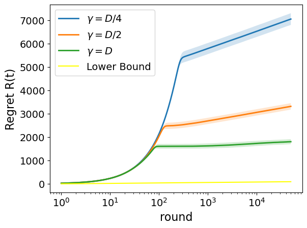
(a) Cyclic communication graph

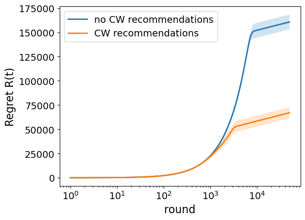
(b) Star communication graph

Figure 5: Group regret for the Sushi dataset using the Message Passing RUCB algorithm and M=100 players. (a) Cyclic communication graph and various values for the decay parameter $\gamma$. (b) Star graph with $\gamma=1$. We compare the Message Passing RUCB algorithm with a similar approach that does not include CW recommendations.

Figure 5a illustrates the group regret per round for the Sushi dataset, employing the message-passing RUCB algorithm with 100 players on a cyclic communication graph. The parameter $\gamma$ is varied to observe its impact on the regret. As $\gamma$ decreases, the slope in the asymptotic region increases, and notably, the case where $\gamma=D$ aligns its slope closest to the lower bound. This alignment corresponds consistently with the findings outlined in Theorem 4.2.

In Figure 5b, we present the regret per round for the Sushi dataset, with M=100 players arranged on a star graph. We compare the performance of the Message Passing RUCB algorithm, as described in Section 4, with and without CW recommendations. Setting the delay to $\gamma=1$ allows us to illustrate the advantage of CW recommendations in quickly identifying the CW. In this scenario, the central player has immediate access to all other players’ observations, while the peripheral players can only utilize their own observations and those of the central player. Consequently, we anticipate that the central player will identify the CW faster than the peripheral players. Once this occurs a CW recommendation will benefit all peripheral players by helping them identify the CW and focus on exploring pairs of arms where at least one arm is the CW. This approach helps address the inherent challenge in the multi-player dueling bandit setting, as discussed in Section 1, which involves exploring non-CW pairs of arms.

Both versions of the Message Passing UCB exhibit similar asymptotic performance. However, as shown in Figure 5b, utilizing CW recommendations leads to a quicker identification of the CW and subsequently results in a much smaller regret. This effect is particularly pronounced in experimental settings where communication graphs have $\gamma<D$.

References

- [1] Agarwal, A. and Ghuge, R. An asymptotically optimal batched algorithm for the dueling bandit problem. Advances in Neural Information Processing Systems, 35:28914–28927, 2022.
- [2] Agarwal, A., Ghuge, R. and Nagarajan, V. Batched dueling bandits. In International Conference on Machine Learning, 89–110, PMLR 2022.
- [3] Arsat, A., Hanafiah, M.H. and Che Shalifullizam, N.I.F. Fast-food restaurant consumer preferences in using self-service kiosks: An empirical assessment of the 4As marketing mix. Journal of Culinary Science and Technology, 1–12, 2023.
- [4] Auer, P., Cesa-Bianchi, N. and Fischer, P. Finite-time analysis of the multiarmed bandit problem. Machine Learning, 47:235–256, 2002.
- [5] Azize, A. and Basu, D. When privacy meets partial information: A refined analysis of differentially private bandits. Advances in Neural Information Processing Systems, 35:32199–32210, 2022.
- [6] Casteigts, A., Métivier, Y., Robson, J.M. and Zemmari, A. Deterministic leader election takes (D+log n) bit rounds. Algorithmica, 81:1901–1920, 2019.
- [7] Cesa-Bianchi, N.O., Gentile, C., Mansour, Y. and Minora, A. Delay and cooperation in nonstochastic bandits. In Conference on Learning Theory, 605–622, PMLR 2016.
- [8] Chawla, R., Sankararaman, A., Ganesh, A. and Shakkottai, S. The gossiping insert-eliminate algorithm for multi-agent bandits. In International Conference on Artificial Intelligence and Statistics, 3471–3481, PMLR 2020.
- [9] Chen, B. and Frazier, P.I. Dueling bandits with weak regret. In International Conference on Machine Learning, 731–739, PMLR 2017.
- [10] De Gemmis, M., Iaquinta, L., Lops, P., Musto, C., Narducci, F. and Semeraro, G. Preference learning in recommender systems. Preference Learning, 41:41–55, 2009.
- [11] Dubey, A. Cooperative multi-agent bandits with heavy tails. In International Conference on Machine Learning, 2730–2739, PMLR 2020.
- [12] Eirinaki, M., Gao, J., Varlamis, I. and Tserpes, K. Recommender systems for large-scale social networks: A review of challenges and solutions. Future Generation Computer Systems, 78:413–418, 2018.
- [13] Jamieson, K., Katariya, S., Deshpande, A. and Nowak, R. Sparse dueling bandits. In Artificial Intelligence and Statistics, 416–424, PMLR 2015.
- [14] Kamishima, T. Nantonac collaborative filtering: recommendation based on order responses. In Proceedings of the Ninth ACM SIGKDD International Conference on Knowledge Discovery and Data Mining, 583–588, 2003.
- [15] Kolla, R.K., Jagannathan, K. and Gopalan, A. Collaborative learning of stochastic bandits over a social network. IEEE/ACM Transactions on Networking, 26(4):1782–1795, 2018.
- [16] Komiyama, J., Honda, J., Kashima, H. and Nakagawa, H. Regret lower bound and optimal algorithm in dueling bandit problem. In Conference on Learning Theory, 1141–1154, PMLR 2015.
- [17] Komiyama, J., Honda, J. and Nakagawa, H. Copeland dueling bandit problem: Regret lower bound, optimal algorithm, and computationally efficient algorithm. In International Conference on Machine Learning, 1235–1244, PMLR 2016.
- [18] Kutten, S., Pandurangan, G., Peleg, D., Robinson, P. and Trehan, A. On the complexity of universal leader election. Journal of the ACM (JACM), 62(1):1–27, 2015.
- [19] Lacerda, B., Gautier, A., Rutherford, A., Stephens, A., Street, C. and Hawes, N. Decision-making under uncertainty for multi-robot systems. AI Communications, 35(4):433–441, 2022.
- [20] Landgren, P., Srivastava, V. and Leonard, N.E. Social imitation in cooperative multiarmed bandits: Partition-based algorithms with strictly local information. In 2018 IEEE Conference on Decision and Control (CDC), 5239–5244, IEEE 2018.
- [21] Landgren, P., Srivastava, V. and Leonard, N.E. Distributed cooperative decision making in multi-agent multi-armed bandits. Automatica, 125:109445, 2021.
- [22] Lattimore, T. and Szepesvári, C. Bandit algorithms. Cambridge University Press, 2020.
- [23] Madhushani, U., Dubey, A., Leonard, N. and Pentland, A. One more step towards reality: Cooperative bandits with imperfect communication. Advances in Neural Information Processing Systems, 34:7813–7824, 2021.
- [24] Mattei, N. and Walsh, T. Preflib: A library for preferences HTTP://WWW. PREFLIB.ORG. In Proceedings of the Third International Conference on Algorithmic Decision Theory (ADT 2013), 259–270, 2013.
- [25] Radlinski, F., Kurup, M. and Joachims, T. How does clickthrough data reflect retrieval quality? In Proceedings of the 17th ACM Conference on Information and Knowledge Management, 43–52, 2008.
- [26] O’Neill J. Open STV. http://www.OpenSTV.org, 2013.
- [27] Rosaci, D., Sarne, G.M. and Garruzzo, S. Muaddib: A distributed recommender system supporting device adaptivity. ACM Transactions on Information Systems (TOIS), 27(4):1–41, 2009.
- [28] Saha, A. and Asi, H. DP-Dueling: Learning from preference feedback without compromising user privacy. arXiv preprint arXiv:2403.15045, 2024.
- [29] Saha, A. and Gaillard, P. Versatile dueling bandits: Best-of-both world analyses for learning from relative preferences. In International Conference on Machine Learning, 19011–19026, PMLR 2022.
- [30] Sankararaman, A., Ganesh, A. and Shakkottai, S. Social learning in multi agent multi armed bandits. Proceedings of the ACM on Measurement and Analysis of Computing Systems, 3(3):1–35, 2019.
- [31] Santoro, N. Design and analysis of distributed algorithms. John Wiley & Sons, 2006.
- [32] Urvoy, T., Clerot, F., Féraud, R. and Naamane, S. Generic exploration and k-armed voting bandits. In International Conference on Machine Learning, 91–99, PMLR 2013.
- [33] Wang, P.A., Proutiere, A., Ariu, K., Jedra, Y. and Russo, A. Optimal algorithms for multiplayer multi-armed bandits. In International Conference on Artificial Intelligence and Statistics, 4120–4129, PMLR 2020.
- [34] Wei, Z., Li, C., Xu, H. and Wang, H. Incentivized communication for federated bandits. Advances in Neural Information Processing Systems, 36:54399–54420, 2023.
- [35] Yang, L., Wang, X., Hajiesmaili, M., Zhang, L., Lui, J. and Towsley, D. Cooperative multi-agent bandits: Distributed algorithms with optimal individual regret and constant communication costs. arXiv preprint arXiv:2308.04314, 2023.
- [36] Yue, Y., Broder, J., Kleinberg, R. and Joachims, T. The k-armed dueling bandits problem. Journal of Computer and System Sciences, 78(5):1538–1556, 2012.
- [37] Yue, Y. and Joachims, T. Interactively optimizing information retrieval systems as a dueling bandits problem. In Proceedings of the 26th Annual International Conference on Machine Learning, 1201–1208, 2009.
- [38] Yue, Y. and Joachims, T. Beat the mean bandit. In Proceedings of the 28th Annual International Conference on Machine Learning, 241–248, 2011.
- [39] Zoghi, M., Karnin, Z.S., Whiteson, S. and De Rijke, M. Copeland dueling bandits. Advances in Neural Information Processing Systems, 28:307-315, 2015.
- [40] Zoghi, M., Whiteson, S., Munos, R. and Rijke, M. Relative upper confidence bound for the k-armed dueling bandit problem. In International Conference on Machine Learning, 10-18, PMLR 2014.