A generalized CDM model with parameterized Hubble parameter in particle creation, viscous and model framework
Abstract
In this study, we construct a theoretical framework based on the generalized Hubble parameter form which may arise within the particle creation, viscous and gravity theory. The Hubble parameter is scrutinized for its compatibility with the observational data relevant to the late-time universe. By using Bayesian statistical techniques based on minimization method, we determine model parameters’s best fit values for the cosmic chronometer and supernovae Pantheon datasets. For the best fit values, the cosmographic and physical parameters are analyzed to understand the cosmic dynamics in model.
Keywords: Flat FLRW metric, Particle creation, Bulk viscosity, Modified gravity.
1 Introduction
The observations of astronomical origin indicates that the universe is expanding with an increasing rate [1, 2, 3]. Subsequently, a desire emerged among theoretical cosmologists to create cosmological models with accelerating phase expansion. At present, the precise nature of enigmatic fluid (or field) that is speeding up the expansion of cosmos is unclear to a great extent. This fluid (or field) is also referred as the ‘dark energy’ [4]. To elucidate the universe’s accelerating expansion, the ‘cosmological constant’ of General relativity model (visualized as the vacuum energy [5]) is widely accepted candidate for dark energy. Although, the cosmological constant appears to fit well with the observational evidences of the universe but this model faces two main problems namely, the coincidence problem and fine tuning problem [4]. There is a nearly -order of magnitude difference between its value from particle physics and the value needed to suit cosmic observations [4].
The universe’s accelerated expansion may be explained by different cosmological mechanisms, see [6, 7, 8, 9, 10]. A modified gravity theory such as the gravity, a barotropic fluid model or a combination of both may be used to describe the early-time and late-time accelerated expansion epochs [6, 7, 8, 9, 10]. An alternative explanation for the accelerated phase can be found in the particle production mechanism also [11, 12]. Schrodinger [13] proposed the particle generation mechanism which further studied by Parker [14, 15]. The particle creation mechanism by an external gravitational field in cosmological modeling has been studied by Parker [16]. There has been lots of discussion on the production of matter in an expanding universe [17, 18, 19, 20, 21, 22, 23, 24, 25]. The particle creation mechanism may yield cosmological scenarios with non-equilibrium thermodynamical descriptions ranging from inflation to late-time acceleration [26].
Viscous fluid presents a compelling and captivating concept within the realms of fluid mechanics [27] and cosmology [28, 29]. Murphy[30] has shown that initial singularity in homogeneous and isotropic Friedmann-Lemaitre-Robertson-Walker (FLRW) cosmology can be resolved by continuous bulk viscosity. The effect of viscosity introduction on the formation of singularity in the Friedmann cosmology framework with the idealized assumption of constant bulk viscosity coefficient has been demonstrated by Heller et al.[31]. Numerous authors have examined the impact of cosmic viscous fluids on universe evolution[32, 33, 24, 34, 35, 36, 37, 38, 39, 40, 41, 42, 43, 44, 45]. The viscous fluids may also pave a way for graceful exit in the early universe during the inflationary epoch [43]. The resolution of the initial singularity problem in mainstream cosmology emphasized in the dynamics of dark matter with bulk viscosity effects [46].
In order to comprehend the different aspects of the observable cosmos, various pioneering concepts have been proposed with the modification of general relativity (GR), see for example [6, 7, 8, 9, 10] and references therein. A fundamental modification originates by replacing the Ricci scalar with a general function of in the Einstein-Hilbert action of GR, known as gravity [47, 48]. The gravity provides a good explanation for the cosmological expansion phenomenon and several studies have examined the limitations of feasible cosmological theories [6, 49]. A number of authors[50, 51, 52] have discussed observational deductions from the models of and, have talked about the solar system’s constraints as well as the astrophysical phenomenon in gravity [53, 54].
In this paper, we show that a parameterized form of Hubble parameter may be a solution in particle creation model. Independently, the considered Hubble parameter may also solved in bulk viscous model and the gravity model. In cosmological modeling, the ansatzes of different cosmological quantities are studied to check whether they admit physically reasonable behaviors or not? The observational viability of ansatzes subjected to the observational data such as the Cosmic chronometer data and Pantheon supernovae data may aid in ruling out different kind of parametrizations. In this paper, we proceed along these lines and show that the cosmological solution based on parameterized Hubble parameter may be physically admitted.
The paper has been arranged in sections as follows: In Sec.(2), the characteristics of cosmological solutions are shown by using a particular Hubble function which may explain the transition from early era deceleration into late-time acceleration. In Section (3), the compatibility of cosmological solution is investigated by using Bayesian statistical techniques with two observational datasets, namely the cosmic chronometer (CC) and Pantheon datasets. In Sec.(4), we show that the considered Hubble parameter may be a solution in cosmological frameworks such as particle creation, viscous fluid model and gravity model. We construct the gravity form and examine the dynamical characteristics of universe in the model. In Sec.(5), we discuss the cosmographic parameters along with the age of current universe in model. Finally, the summary and conclusions are given in Sec.(6).
2 The cosmological equations and background dynamics
The astronomical observations about the expanding universe points that the rate of universe’s expansion is increasing although its spatial geometry seems be almost flat [3]. It is also well-established that the universe expansion history has a past of decelerating expansion which transits into the accelerating expansion phase during present times. For the observable universe, as par Aghanim et al. [3] the present day value of the expansion rate is . Homogeneous and isotropic universe’s expansion rate is described by , where denotes the scale factor and overhead dot is time derivative. The spatially flat metric for homogeneous and isotropic universe may be written as
| (1) |
In the general relativity context, the field equations can be expressed as
| (2) |
where and represent the energy density and pressure respectively. In order to understand the transitional universe expansion era, we adopt a parametrization of the Hubble parameter . The parametrizations may be used in a model-independent manner for exploring the characteristics of dark energy dominated universe. Different kind of parameterization when tested against the observational data may single out the physically reasonable cases. In this approach, we proceed with the Hubble parameter having form
| (3) |
Here, represents the Hubble parameter’s current value and , are arbitrary constants. The above Hubble parameter may be seen as the generalization of cold dark matter model defined by . Although, the CDM model is supported by the latest observational datasets [1, 3, 55, 56, 57], the cosmological studies based on parametrizations of different parameters are widely explored [10, 18, 19, 20, 21, 22, 23, 24, 25, 26, 32, 33, 34, 35, 36, 37, 38, 39, 40, 41, 42, 43, 58, 59, 60, 61, 62]. Above equation (3) may be solved using the relation with standard convention for present era to obtain Hubble parameter in terms of red-shift () as
| (4) |
This kind of Hubble parameter may arise with affine equation of state , where are some constant [61] or in modified theory of gravity [58, 62]. When it comes to understanding the dynamics of the cosmic universe the cosmographical parameter with the most influential is thought to be . Based on the values of this parameter, the expansion dynamics of universe may be categorized into either accelerated or decelerated phases with representing the transitional periods. The universe exhibits deceleration when and power-law expansion when . The universe exhibits super-exponential (de Sitter) expanding era for () respectively. This cosmographic parameter may be defined as and by using equation (4), we obtain
| (5) |
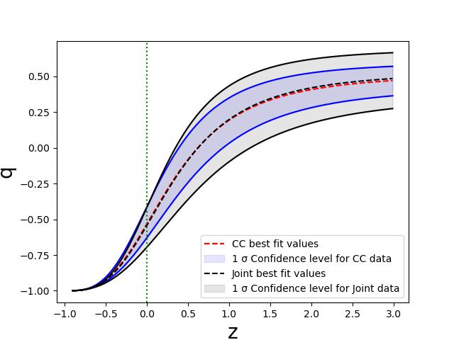
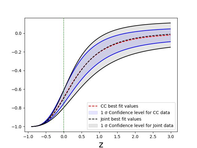
Based on the model parameters’ best fit values (see section 3), the evolution of deceleration parameter and effective equation of state (EoS) parameter of the reconstructed universe is shown in figure (2) and (2) respectively. For our model, the values of deceleration parameter are (for the CC data) and (for the joint data) at present time having .
3 Observational constraints on model
In this part, we examine the compliance of parameterized from of Hubble parameter with datasets of the cosmic chronometer (CC) and the joint data consisting of Pantheon and cosmic chronometer data nomenclated (in present paper) as CC+Pantheon sample. In order to perform statistical analysis, we use minimization method with the Markov Chain Monte Carlo (MCMC) technique implemented with the emcee tool [63] and constrain the parameters to study of the cosmic behavior in the model.
3.1 The Cosmic chronometer data
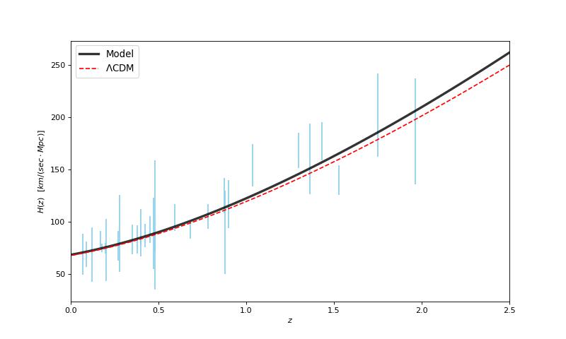
The values of Hubble parameter at any instant describes the expansion rate of the universe at that particular instant and its observational values are important for exploration of dark energy and the evolution of universe. To constrain the model parameters, we use Cosmic Chronometer data composed of 31 data points [64, 65] which are determined by differential ages of galaxies technique within the red-shift region .
In this case, we minimize the function and thus the model parameters are estimated with their best fit values. The corresponding may be expressed as
| (6) |
where the observed values are denoted by and theoretical values of the Hubble parameter are denoted by . The values are the standard deviation for each observed value.
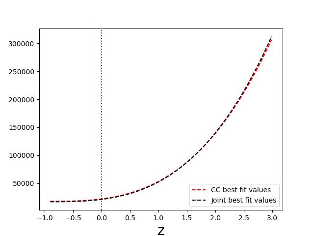
Figure illustrates the error bars of the CC points with the best fit Hubble parameter curve for the Hubble parameter (Eq. (4)).
3.2 The Pantheon data
We use the Pantheon sample, which includes supernovae Type Ia (SNIa) data points for the red-shift range [66]. The CfA1-CfA4 [67, 68] surveys, Pan-STARRS1 Medium Deep Survey [66], SDSS [69], SNLS [70], Carnegie Supernova Project (CSP) [71] contributes to the SNIa sample. For the MCMC analysis using Pantheon data, the theoretically expected apparent magnitude is given by
| (7) |
where is the absolute magnitude. Also, the luminosity distance (having dimension of the Length) may be defined as [72]
| (8) |
where represents SNIa’s red-shift as determined in the cosmic microwave background (CMB) rest frame and and is the speed of light. The luminosity distance is typically substituted with the dimensionless Hubble-free luminosity distance given by . The equation (7) could also be rewritten as
| (9) |
The parameters and can be combined to create a new parameter , which may be identified as
| (10) |
where . We use this parameter with pertinent for Pantheon data in the MCMC analysis as [73]
| (11) |
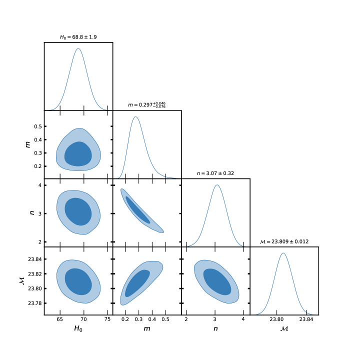
where , is the covariance matrix’s inverse and will be provided by equation (9). The luminosity distance depends on the Hubble parameter. Therefore, we use the emcee package [63] and equation (4) to get the maximum likelihood estimate using the joint CC+Pantheon data set. The joint for maximum likelihood estimate may be defined as . In Fig. , we displays the marginalized and contour map and D posterior distribution from the Monte Chain Monte Carlo analysis using CC+Pantheon data. The Table (1) summarizes the best fit values for the model parameters in the MCMC analysis for the model.
| Dataset | m | n | ||
|---|---|---|---|---|
| CC | - | |||
| CC+Pantheon |
4 The parameterized Hubble parameter as cosmological solution in different frameworks
4.1 The Particle Creation model
With the FLRW spacetime, the fundamental cosmological equations with the particle creation mechanism in a model may be written as
| (12) |
where and represent to the thermodynamic pressure of the matter content and energy density respectively with is representing the creation pressure. The fluid particles are not conserved if thermodynamic system is regarded as open (, where particle number density is represented by , while the fluid flow vector is denoted by ). The particle conservation equation can be expressed as follows,
| (13) |
where the particle production rate is the rate of change in particle number in the co-moving volume . Depending on the particle production rate, one may identify the creation or annihilation of particles. Particle creation occurs when , particle annihilation occurs when , and no particle production occurs when . According to the second law of thermodynamics, is required for entropy to never decrease. The gravitationally induced adiabatic particle formation rate and creation pressure are related by the relation[74, 75].
| (14) |
When particle production is present or absent, the creation pressure is negative or zero respectively. The energy conservation equation may be expressed as
| (15) |
By considering the universe with matter having , the energy density of matter may be written using Eqs. (4), (12) and (15) as
| (16) |
In this scenario, the particle creation rate may be written as using Eqs. (4), (12), (14) as
| (17) |
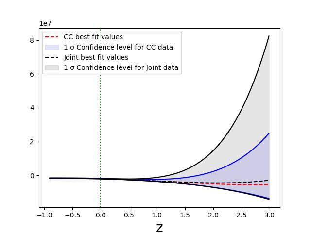
The above derived particle creation rate may interpolate between the early decelerating era with the late-time accelerating era in the model. The creation pressure being negative from the recent past may yield the mechanism for accelerating universe expansion in model. Matter’s energy density behavior and creation pressure have been displayed in Fig. (6) and (6) respectively. The energy density remains positive during different cosmological evolution eras while the creation pressure has become negative from the recent past.
4.2 Bulk viscous model
For the FRW metric (1), the field equations in the bulk viscous fluid model are
| (18) |
where the bulk viscous pressure may be written as
| (19) |
with being coefficient of bulk viscosity with and denoting the energy density and pressure of fluid respectively. In this paper, we consider the generic form of the inhomogeneous viscous fluid having form , where the bulk viscosity is a general function of , and it’s derivatives. The continuity equation may be expressed as
| (20) |
where is a natural candidate for actual fluid and contributes to the dissipative effects. By considering the matter having , the ernergy density and viscous pressure may take the form
| (21) |
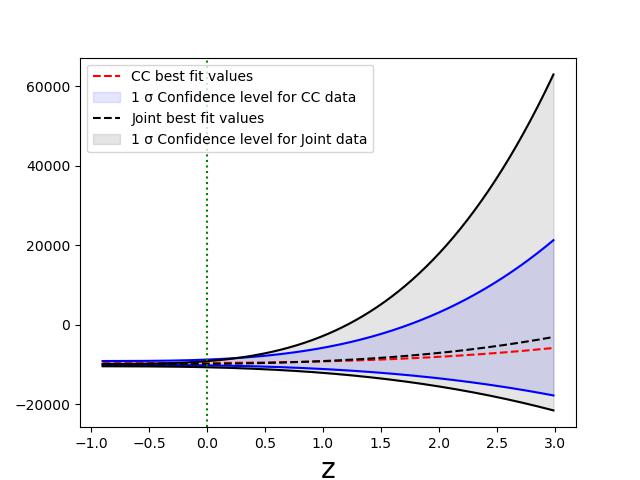
The Fig. depict the evolution of bulk viscous pressure with red-shift. We can easily observe that bulk viscous pressure has negative values which may be responsible for accelerating universe expansion in the model.
4.3 The gravity model reconstruction
The gravity theory action may be written as
| (22) |
where denotes a general function of the Ricci scalar and the action for the appropriate matter distribution is denoted by . The field equation may result by varying action (22) with respect to the metric tensor as
| (23) |
where and is stress-energy tensor. The field equations of gravity can be expressed in terms of the Einstein tensor, which includes an effective energy–momentum tensor .
| (24) |
The Raychaudhuri equation in gravity for a time-like congruence with velocity vector may take the form [76, 77]
| (25) |
The last term that is located on the right-hand side of equation (25) can be expressed as follows using the field equations (23) for theory:
| (26) |
In this paper, we are dealing with the homogeneous and isotropic, spatially flat universe given by the metric (1). The Raychaudhuri equation (25) takes the following form for such a metric and a matter distribution of a perfect fluid as [78, 79]
| (27) |
It should be emphasized that for the fluid distribution, we have not assumed any equation of state until now, but by using field equations (24) in the Raychaudhuri equation (25) as to eliminates the fluid pressure .
In principle, the function of this modified gravity may be determined by using either the Hubble parameter or the scale factor. By using equation (27), we aim to determine gravity form for the Hubble parameter 3. The Ricci scalar for a spatially flat Friedmann-Robertson-Walker metric (1) is . Using the equation (3), we can write
| (28) |
Here and . Using the equation (3), (27) and (28), we obtain
| (29) |
For the matter having pressure , the energy density may be given by and thus above Eq. (4.3) may take the form
| (30) |
Solving Eq. (4.3), we obtained one solution for as
| (31) |
where , and . We may also have the energy density of the matter given by
| (32) |
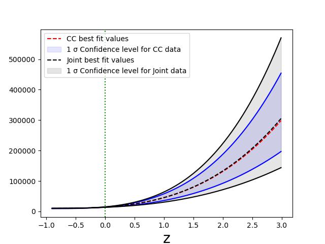
For the best fit values given in Table (1), the behavior of energy density with red-shift have been displayed in Fig. (8). The energy density remains positive during the decelerating era and will preserve its positive nature as the universe evolves into the accelerating era in model.
5 General issues
In this section, we study the cosmographic evolution of the universe governed by Hubble parameter (3). The cosmographic parameter helps to identify the sharp contrast between the dark energy energy model and the CDM model. We also identify the universe’s age in model for the best fit values in model.
5.1 Cosmographic parameters
The kinematic quantities like as jerk and snap parameter defines the cosmic scenario by using the geometric quantities like as the scale factor and its derivatives. The cosmography study was initially discussed by Weinberg [80] by using a Taylor series to introduce the scale factor that increased around present time . The Hubble parameter is regarded as a changeable observable quantity prior to discovering evidence of the Universe’s accelerating expansion. The deceleration parameter illustrates its evolution, by using the second-order derivative of [81]. The snap and jerk parameters provide insights about the cosmic evolution of the universe. Jerk can also sometimes be referred to as jolt, and jounce is another word for snap and may be defined as [82]:
| (33) |
For and , the previous equation (33) can be rewritten in red-shift’s terms as [83].
| (34) |
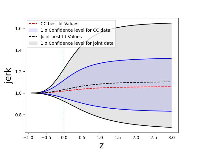
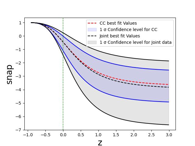
For the best fit parameter values, the jerk and snap parameter behaviors have been illustrated in figure and respectively. The snap and jerk parameters are provided by and respectively, for the best fit values derived from the CC data set. The values of the jerk parameter differ from the CDM model with . The obtained values of jerk and snap parameters respectively are , for the best fit values derived from for joint data set.
5.2 Age of the Universe
In a cosmological model, the cosmic age of the universe can be calculated as
| (35) |
We numerically calculate the aforementioned integral and get the present age of the universe for and use the Hubble parameter (Eq. 3). For this model, the obtained value of universe’s present age is Gyr for CC data and Gyr which are very close to the present age values obtained from the recent observations [3].
6 Conclusions
In this paper, we investigated the a cosmological model having homogeneous and isotropic line element with flat spatial sections and a parameterized form of Hubble parameter. This kind of Hubble parameter may interpolate between the decelerating past to the accelerating present of the universe. We show that that this kind of Hubble parameter may be a solution in the particle creation, bulk viscous, and gravity framework of cosmological modeling for , and respectively where are some constants containing constrained model parameters. The Raychaudhuri equation has been used to get the form of function in the model.
We scrutinize the observational viability of considered Hubble parameter form to the Cosmic chronometer and Pantheon data. By using Bayesian statistical technique with MCMC analysis, we obtain model parameters’s best fit values. The obtained best fit are , , subjected to the CC data and , , subjected to the joint data of CC+Pantheon sample. At last, we find universe’s present age is Gyr for CC data and Gyr for joint CC+Pantheon data.
Furthermore, the behavior of cosmographic parameters suggest that the universe in model will behave like CDM model as . The early phase of the universe evolution is decelerating in nature which has been transitioned into the accelerating phase (see Figs. (2) and (2). According to model parameters best fit values, the transition red-shift is . Additionally for our model, the present values of deceleration parameter are (for the CC data) and (for the CC+Pantheon data). The universe is dominated by the cold dark matter-like component at large red-shifts and subsequently the universe expands under the influence of quintessence kind of dark energy and will eventually approaches the cosmological constant limit having as .
It is evident in the model that the energy density will be decreasing with time while preserving positive nature during the complete cosmological history. From the trends obtained according to the observational data, the value of jerk parameter decreases from early to late times and, finally approaches to which demonstrates that, in the early universe this model differs from the CDM model and becomes similar to CDM model in later times. Additionally, the jerk parameter’s current values are for the CC data and for the CC+Pantheon data. In the early cosmos, the snap parameter () develops in the negative region. The values of snap parameter at the present times are for the CC data and for the CC+Pantheon data.
In summary, we show that the parameterized Hubble parameter cosmology may be a observationally viable one and, it may be admitted as a solution in the particle creation, bulk viscous, and gravity framework also.
Acknowledgments
G.P. Singh and A. Singh thanks the Inter-University Centre for Astronomy and Astrophysics (IUCAA), Pune, India for support under the Visiting Associateship programme.
References
- [1] A. G. Riess et al., Observational Evidence from Supernovae for an Accelerating Universe and a Cosmological Constant, Astronomical Journal 116 (3) (1998) 1009–1038.
- [2] S. Perlmutter et al., Measurements of and from 42 High-Redshift Supernovae, Astrophysical Journal 517 (2) (1999) 565–586.
- [3] N. Aghanim et al., [Planck Collaboration], Planck 2018 results. VI. Cosmological parameters, Astronomy and Astrophysics 641 (2020) A6.
- [4] E. J. Copeland, M. Sami, S. Tsujikawa, Dynamics of dark energy, International Journal of Modern Physics D 15 (11) (2006) 1753–1935.
- [5] S. Weinberg, The cosmological constant problem, Reviews of modern physics 61 (1) (1989) 1.
- [6] S. Capozziello, et al., Cosmological viability of gravity as an ideal fluid and its compatibility with a matter dominated phase, Physics Letters B 639 (3-4) (2006) 135–143.
- [7] S. Nojiri, S. D. Odintsov, Introduction to modified gravity and gravitational alternative for dark energy, International Journal of Geometric Methods in Modern Physics 4 (01) (2007) 115–145.
- [8] S. Nojiri, S. D. Odintsov, Unified cosmic history in modified gravity: from theory to lorentz non-invariant models, Physics Reports 505 (2-4) (2011) 59–144.
- [9] K. Bamba, et al., Dark energy cosmology: the equivalent description via different theoretical models and cosmography tests, Astrophysics and Space Science 342 (2012) 155–228.
- [10] K. Bamba, et al., Inflationary universe from perfect fluid and gravity and its comparison with observational data, Physical Review D 90 (12) (2014) 124061.
- [11] L. Abramo, J. Lima, Inflationary models driven by adiabatic matter creation, Classical and Quantum Gravity 13 (11) (1996) 2953.
- [12] W. Zimdahl, Cosmological particle production, causal thermodynamics, and inflationary expansion, Physical Review D 61 (8) (2000) 083511.
- [13] E. Schrodinger, The proper vibrations of the expanding universe, Physica 6 (7-12) (1939) 899–912.
- [14] L. Parker, Particle creation in expanding universes, Physical Review Letters 21 (8) (1968) 562.
- [15] L. Parker, Quantized fields and particle creation in expanding universes. , Physical Review D 3 (2) (1971) 346.
- [16] L. Parker, Quantized fields and particle creation in expanding universes. i, Physical Review 183 (5) (1969) 1057.
- [17] R. Durrer, K. E. Kunze, M. Sakellariadou, Particle creation in pre-big-bang cosmology, New Astronomy Reviews 46 (11) (2002) 659–680.
- [18] G. P. Singh, A. Beesham, Bulk viscosity and particle creation in brans–dicke theory, Australian journal of physics 52 (6) (1999) 1039–1049.
- [19] G. P. Singh, A. Beesham, R. V. Deshpande, Particle production in higher derivative theory, Pramana 54 (2000) 729–736.
- [20] A. Singh, A complete cosmological scenario with particle creation, Astrophysics and Space Science 365 (3) (2020) 54.
- [21] N. Hulke, et al., Variable chaplygin gas cosmologies in gravity with particle creation, New Astronomy 77 (2020) 101357.
- [22] G. P. Singh, R. V. Deshpande, T. Singh, Viscous cosmological models with particle creation in brans-dicke theory, Astrophysics and space science 282 (2002) 489–498.
- [23] G. P. Singh, A. Y. Kale, Anisotropic bulk viscous cosmological models with particle creation, Astrophysics and Space Science 331 (2011) 207–219.
- [24] R. Chaubey, Bianchi type-v bulk viscous cosmological models with particle creation in brans-dicke theory, Astrophysics and Space Science 342 (2) (2012) 499–509.
- [25] G. P. Singh, A. R. Lalke, N. Hulke, Study of particle creation with quadratic equation of state in higher derivative theory, Brazilian Journal of Physics 50 (2020) 725–743.
- [26] S. Chakraborty, S. Saha, Complete cosmic scenario from inflation to late time acceleration: Nonequilibrium thermodynamics in the context of particle creation, Physical Review D 90 (12) (2014) 123505.
- [27] L. Landau, E. M. Lifshitz, Fluid mechanics, Pregamon Press, Oxford, (1987).
- [28] C. W. Misner, Transport processes in the primordial fireball, Nature 214 (5083) (1967) 40–41.
- [29] S. Weinberg, Entropy generation and the survival of protogalaxies in an expanding universe, Astrophysical Journal 168 (1971) 175.
- [30] G. L. Murphy, Big-bang model without singularities, Physical Review D 8 (12) (1973) 4231.
- [31] M. Heller, Z. Klimek, L. Suszycki, Imperfect fluid friedmannian cosmology, Astrophysics and Space Science 20 (1973) 205–212.
- [32] T. Singh, R. Chaubey, A. Singh, Bouncing cosmologies with viscous fluids, Astrophysics and Space Science 361 (2016) 1–5.
- [33] G. P. Singh, N. Hulke, A. Singh, Thermodynamical and observational aspects of cosmological model with linear equation of state, International Journal of Geometric Methods in Modern Physics 15 (08) (2018) 1850129.
- [34] R. Chaubey, et al., The general class of bianchi cosmological models in f (r, t) gravity with dark energy in viscous cosmology, Indian Journal of Physics 90 (2016) 233–242.
- [35] A. Singh, R. Chaubey, Unified and bouncing cosmologies with inhomogeneous viscous fluid, Astrophysics and Space Science 366 (1) (2021) 15.
- [36] G. P. Singh, B. K. Bishi, Bulk viscous cosmological model in brans-dicke theory with new form of time varying deceleration parameter, Advances in High Energy Physics 2017 (2017).
- [37] G. P. Singh, B. K. Bishi, Hypersurface-homogeneous bulk viscous cosmological models with particle creation in general relativity, Iranian Journal of Science and Technology, Transactions A: Science 41 (2017) 809–817.
- [38] R. Raushan, et al., Universe with quadratic equation of state: A dynamical systems perspective, International Journal of Geometric Methods in Modern Physics 17 (05) (2020) 2050064.
- [39] A. Singh, et al., Lagrangian formulation and implications of barotropic fluid cosmologies, International Journal of Geometric Methods in Modern Physics 19 (07) (2022) 2250107.
- [40] A. Singh, R. Raushan, R. Chaubey, On the anisotropic bouncing universe with viscosity, International Journal of Geometric Methods in Modern Physics 20 (12) (2023) 2350201.
- [41] A. Singh, Homogeneous and anisotropic cosmologies with affine eos: a dynamical system perspective, European Physical Journal C 83 (08) (2023) 696.
- [42] M. Sharif, R. Saleem, Effects of viscous pressure on warm inflationary generalized cosmic chaplygin gas model, Journal of Cosmology and Astroparticle Physics 2014 (12) (2014) 038.
- [43] R. Myrzakulov, L. Sebastiani, Inhomogeneous viscous fluids for inflation, Astrophysics and Space Science 356 (2015) 205–213.
- [44] A. Pradhan, A. Dixit, M. Zeyauddin, Reconstruction of cdm model from f(t) gravity in viscous-fluid universe with observational constraints, International Journal of Geometric Methods in Modern Physics 21 (01) (2024) 2450027.
- [45] A. Pradhan, A. Dixit, D. C. Maurya, Quintessence behavior of an anisotropic bulk viscous cosmological model in modified f(q)-gravity, Symmetry 14 (12) (2022).
- [46] M. Szydłowski, A. Krawiec, Viscous matter in frw cosmology, Symmetry 12 (8) (2020) 1269.
- [47] H. A. Buchdahl, Non-linear lagrangians and cosmological theory, Monthly Notices of the Royal Astronomical Society 150 (1) (1970) 1–8.
- [48] R. Kerner, Cosmology without singularity and nonlinear gravitational Lagrangians., General Relativity and Gravitation 14 (5) (1982) 453–469.
- [49] L. Amendola, D. Polarski, S. Tsujikawa, Are f (r) dark energy models cosmologically viable?, Physical review letters 98 (13) (2007) 131302.
- [50] A. A. Starobinsky, Disappearing cosmological constant in f (r) gravity, JETP letters 86 (2007) 157–163.
- [51] S. Capozziello, S. Tsujikawa, Solar system and equivalence principle constraints on f (r) gravity by the chameleon approach, Physical Review D 77 (10) (2008) 107501.
- [52] T. Liu, X. Zhang, W. Zhao, Constraining f (r) gravity in solar system, cosmology and binary pulsar systems, Physics Letters B 777 (2018) 286–293.
- [53] S. Capozziello, V. Cardone, V. Salzano, Cosmography of f (r) gravity, Physical Review D 78 (6) (2008) 063504.
- [54] G. P. Singh, N. Hulke, A. Singh, Cosmological study of particle creation in higher derivative theory, Indian Journal of Physics 94 (1) (2020) 127–141.
- [55] S. Perlmutter, et al., Discovery of a supernova explosion at half the age of the universe, Nature 391 (6662) (1998) 51–54.
- [56] D. J. Eisenstein, W. Hu, M. Tegmark, Cosmic complementarity: H0 and m from combining cosmic microwave background experiments and redshift surveys, Astrophysical Journal 504 (2) (1998) L57.
- [57] B. S. Haridasu, et al., Strong evidence for an accelerating universe, Astronomy & Astrophysics 600 (2017) L1.
- [58] D. C. Maurya, Transit cosmological model with specific hubble parameter in f(r, t) gravity, New Astronomy 77 (2020) 101355.
- [59] S. Mandal, A. Singh, R. Chaubey, Observational constraints and cosmological implications of nle model with variable g, European Physical Journal Plus 137 (11) (2022) 1246.
- [60] A. R. Lalke, G. P. Singh, A. Singh, Cosmic dynamics with late-time constraints on the parametric deceleration parameter model, European Physical Journal Plus 139 (03) (2024) 288.
- [61] A. Singh, S. Krishnannair, Affine eos cosmologies: Observational and dynamical system constraints, Astronomy and Computing 47 (2024) 100827.
- [62] D. C. Maurya, Quintessence behaviour dark energy models in f(q,b)-gravity theory with observational constraints, Astronomy and Computing 46 (2024) 100798.
- [63] D. Foreman-Mackey et al., emcee: the mcmc hammer, Publications of the Astronomical Society of the Pacific 125 (925) (2013) 306.
- [64] G. S. Sharov, V. O. Vasiliev, How predictions of cosmological models depend on hubble parameter data sets, arXiv preprint arXiv:1807.07323 (2018).
- [65] J. Simon, L. Verde, R. Jimenez, Constraints on the redshift dependence of the dark energy potential, Physical Review D 71 (12) (2005) 123001.
- [66] D. M. Scolnic, et al., The complete light-curve sample of spectroscopically confirmed sne ia from pan-starrs1 and cosmological constraints from the combined pantheon sample, Astrophysical Journal 859 (2) (2018) 101.
- [67] A. G. Riess, et al., Bvri light curves for 22 type ia supernovae, Astronomical Journal 117 (2) (1999) 707.
- [68] M. Hicken, et al., Improved dark energy constraints from 100 new cfa supernova type ia light curves, Astrophysical Journal 700 (2) (2009) 1097.
- [69] M. Sako, et al., The data release of the sloan digital sky survey-ii supernova survey, Publications of the Astronomical Society of the Pacific 130 (988) (2018) 064002.
- [70] J. Guy, et al., The supernova legacy survey 3-year sample: Type ia supernovae photometric distances and cosmological constraints, Astronomy & Astrophysics 523 (2010) A7.
- [71] C. Contreras, et al., The carnegie supernova project: first photometry data release of low-redshift type ia supernovae, Astronomical Journal 139 (2) (2010) 519.
- [72] S. D. Odintsov, et al., Cosmological fluids with logarithmic equation of state, Annals of Physics 398 (2018) 238–253.
- [73] K. Asvesta, et al., Observational constraints on the deceleration parameter in a tilted universe, Monthly Notices of the Royal Astronomical Society 513 (2) (2022) 2394–2406.
- [74] M. O. Calvao, J. A. S. Lima, I. Waga, On the thermodynamics of matter creation in cosmology, Physics Letters A 162 (3) (1992) 223–226.
- [75] J. A. S. Lima, A. S. M. Germano, On the equivalence of bulk viscosity and matter creation, Physics Letters A 170 (5) (1992) 373–378.
- [76] A. Raychaudhuri, Relativistic cosmology. i, Physical Review 98 (4) (1955) 1123.
- [77] J. Ehlers, Contributions to the relativistic mechanics of continuous media, General Relativity and Gravitation 25 (1993) 1225–1266.
- [78] A. Guarnizo, L. Castañeda, J. M. Tejeiro, Geodesic deviation equation in f(r) gravity, General Relativity and Gravitation 43 (2011) 2713–2728.
- [79] S. Gupta Choudhury, A. Dasgupta, N. Banerjee, Reconstruction of gravity models for an accelerated universe using the raychaudhuri equation, Monthly Notices of the Royal Astronomical Society 485 (4) (2019) 5693–5699.
- [80] S. Weinberg, Cosmology (2008).
- [81] A. Mukherjee, N. Banerjee, Parametric reconstruction of the cosmological jerk from diverse observational data sets, Physical Review D 93 (4) (2016) 043002.
- [82] M. Visser, Jerk, snap and the cosmological equation of state, Classical and Quantum Gravity 21 (11) (2004) 2603.
- [83] F. Wang, Z. Dai, S. Qi, Probing the cosmographic parameters to distinguish between dark energy and modified gravity models, Astronomy & Astrophysics 507 (1) (2009) 53–59.