Nonlinear denoising score matching for enhanced learning of structured distributions

Abstract

We present a novel method for training score-based generative models which uses nonlinear noising dynamics to improve learning of structured distributions. Generalizing to a nonlinear drift allows for additional structure to be incorporated into the dynamics, thus making the training better adapted to the data, e.g., in the case of multimodality or (approximate) symmetries. Such structure can be obtained from the data by an inexpensive preprocessing step. The nonlinear dynamics introduces new challenges into training which we address in two ways: 1) we develop a new nonlinear denoising score matching (NDSM) method, 2) we introduce neural control variates in order to reduce the variance of the NDSM training objective. We demonstrate the effectiveness of this method on several examples: a) a collection of low-dimensional examples, motivated by clustering in latent space, b) high-dimensional images, addressing issues with mode collapse, small training sets, and approximate symmetries, the latter being a challenge for methods based on equivariant neural networks, which require exact symmetries.

1 Introduction

Since the introduction of score-based generative models (SGMs) [Song et al., 2020, Ho et al., 2020] there has been intense interest in accelerating their training and generation processes. While being able to produce high quality images with minimal mode collapse [Xiao et al., 2021], SGM’s generation process is comparably more expensive than generative adversarial nets [Goodfellow et al., 2014] or normalizing flows Grathwohl et al. [2018]. In this paper, we introduce and develop the use of nonlinear forward processes in SGMs. While the original formulation of SGMs by Song et al. [2020] included the possibility of nonlinear forward processes, their practical use has neither been well-explored, nor justified due to the great empirical success of linear forward processes. We find that, when designed wisely, nonlinear diffusion processes provide a way to incorporate structure about the target distribution, such as multimodality or approximate symmetry, into the SGM to produce higher quality samples with less data.

The class of forward processes we consider is inspired by overdamped Langevin dynamics (OLD). SGMs that use the Ornstein-Uhlenbeck process, the OLD of the normal distribution, as the forward process have been widely explored. In this work, we use more general OLD corresponding to Gaussian mixture models (GMM). These GMMs can be learned cheaply via a preprocessing step on a subset of (unlabeled or sparsely labeled) data, and then used to define the drift for the forward process. The use of GMMs is well-motivated for SGMs. Gold standard implementations of generative models [Vahdat et al., 2021, Rombach et al., 2022] perform SGMs in the latent space. As distributions in the latent space are often multimodal in scientific applications [Ding et al., 2019, Li et al., 2023], we argue GMMs are a natural choice for nonlinear forward processes. Furthermore, nonlinear drift terms based on OLDs corresponds with choosing reference measures other than the Gaussian. Via the optimal control interpretation of SGM [Berner et al., 2022, Zhang and Katsoulakis, 2023] we can also interpret the nonlinear drift term as arising from a state cost in the control problem.

Denoising score-matching (DSM) [Vincent, 2011, Song et al., 2020] is the most frequently used objective function for learning the score function as it avoids computing derivatives of the score. Their use, however, relies on knowing the probability transition kernel of the forward process, which is only possible for linear processes. Therefore, we develop a nonlinear version of DSM (NDSM) in Section 3. The main idea is that even for nonlinear drift functions, the local transition probability functions are approximately normal. Robustly implementing NDSM is a challenge in itself, and relies on a novel neural control variates method to produce low variance estimates of the objective function. Neural control variates are a deep learning version of classical control variates [Asmussen and Glynn, 2007], for variance reduction, and may be of independent interest elsewhere.

Numerical experiments on MNIST and its approximate $C_{2}$-symmetric variant validate our theoretical arguments. In particular, in Table 2, we see that the inception score and FID with our model vastly outperforms the standard OU with DSM SGM. Moreover, we also show our model can learn generative models with substantially less data, as shown in Figure 1.

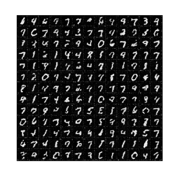
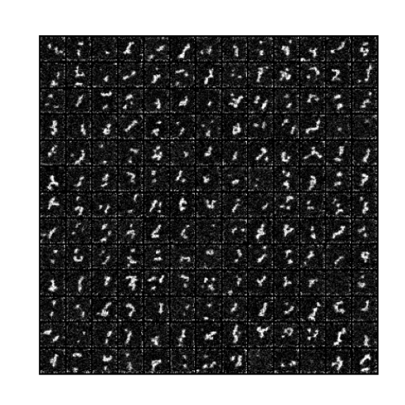
(a) $N=6000$: NDSM (left), DSM (right)

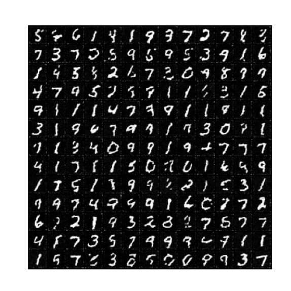
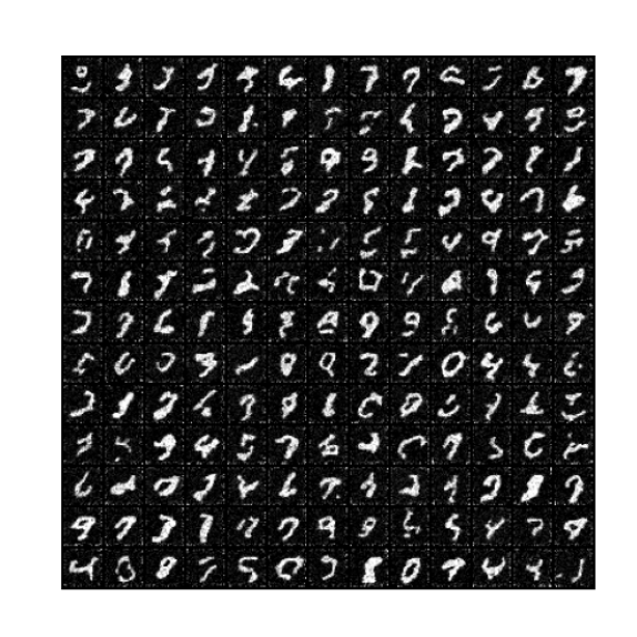
(b) $N=14000$: NDSM (left), DSM (right)

Figure 1: MNIST in the low data regime ($N$ training samples), comparing OU+DSM with our new GM+NDSM-CV method. GM+NDSM-CV can learn well with less data.

1.1 Contributions

• We introduce score-based generative modeling with nonlinear forward noising processes for enhanced learning of distributions with structure. Specifically, an inexpensive preprocessing step is applied to (a subset of) the data to construct a Gaussian mixture (GM) reference measure. This reference measure constitutes the initial distribution of the denoising process and also determines the nonlinear drift of the forward noising process. The GM nonlinear drift, being informed by the structure of the data, then leads to improved performance.

• NDSM, a nonlinear version of the denoising score-matching objective function, is introduced to facilitate the practical implementation SGMs with nonlinear drift term. A robust implementation of NDSM relies on a novel neural control variates method.

• Numerical experiments validate our claims of improved performance, including better FID and inceptions scores as well as a reduction in mode collapse and the ability to learn from fewer training samples.

2 Score-based generative models with nonlinear noising dynamics

Let $\pi$ be the target data distribution on ${\mathbb{R}}^{d}$ known only through a finite set of samples $\{y_{i}\}_{i=1}^{N}$. Score-based generative modeling considers a pair of diffusion processes whose evolution are time reversals of each other. Given a drift vector field $f:[0,T]\times{\mathbb{R}}^{d}\to{\mathbb{R}}^{d}$ and a diffusion coefficient $\sigma:[0,T]\to{\mathbb{R}}$, these diffusion processes $Y(s)$ and $X(t)$ are defined on the time interval $s,t\in[0,T]$ by

$$\begin{dcases}dY(s)=-f(Y(s),T-s)ds+\sigma(T-s)dW(s),\,\,\,\,Y(0)\sim\pi\\ dX(t)=(f(X(t),t)+\sigma(t)^{2}\nabla\log\eta(T-t,X(t)))dt+\sigma(t)dW(t),\,\,\,\,X(0)\sim\rho_{0},\end{dcases}$$ (1)

where $Y(s)\sim\eta(s,\cdot)$ and $\rho_{0}$ is some initial reference measure. If $\rho_{0}=\eta(T,\cdot)$, then $X(t)$ exactly follows the time reversed evolution of $Y(s)$, i.e., $X(t)\sim\eta(T-t,\cdot)$. Typically, $f$ and $\sigma$ are chosen such that $Y(s)$ evolves to a Gaussian as quickly as possible. Linear SDEs such as the Ornstein-Uhlenbeck process (OU) ($f(x,t)=x/2$, $\sigma(t)=1$), “variance exploding” processes ($f(t,x)=0$, with $\sigma(t)$ growing quickly in $t$), or the critically damped Langevin process Dockhorn et al. [2021], are the most common choices in practice. Moreover, the score function is learned via a score-matching (SM) objective, typically the denoising SM.

We choose nonlinear noising dynamics arising from the overdamped Langevin dynamics Pavliotis [2014]. If the noising process corresponded with a Langevin process with stationary distribution $\rho_{0}\propto\exp(-V(x))$, then it would correspond to a drift term $f=-\nabla V(x)$ and $\sigma(t)=\sqrt{2}$. In this paper, we choose $\rho_{0}$ to be a Gaussian mixture model (GMM), and choose the nonlinear noising dynamics accordingly. However, we emphasize that the NDSM method we develop can be applied to any nonlinear drift.

2.1 Gaussian mixture forward dynamics

We use the freedom to choose the drift, $f$, in (1) to match the noising dynamics to the structure of the data. Specifically, we fit a GMM with weights $w_{i}$, means $\mu_{i}$, and covariances $\Sigma_{i}$ to (a subset of) the data, in an inexpensive preprocessing step; we note that the the required preprocessing does not require labeled data. The density

$$\eta_{*}(y)=\sum_{i=1}^{K}w_{i}N_{\mu_{i},\Sigma_{i}}(y)\,,\,\,\,N_{\mu_{i},\Sigma_{i}}(y)\coloneqq(2\pi)^{-d/2}\det(\Sigma_{i})^{-1/2}\exp\left(-\frac{(y-\mu_{i})\cdot\Sigma_{i}^{-1}(y-\mu_{i})}{2}\right)$$ (2)

is then invariant under the GM noising dynamics

$$dY(s)=-\nabla V(Y(s))ds+\sqrt{2}dW(s),\quad V(y)\coloneqq-\log\left[\sum_{i=1}^{K}w_{i}N_{\mu_{i},\Sigma_{i}}(y)\right].$$ (3)

The noising dynamics (3), together with the corresponding denoising dynamics and initial distribution $\rho_{0}=\eta_{*}$, encodes important aspects of the structure of the data, such as multimodality and (approximate) symmetries. We demonstrate that this leads to improved performance, especially when using a small training set, and also helps to prevent mode collapse. Pseudocode for the corresponding noising and denoising dynamics, using the Euler-Maruyama (EM) discretization can be found in Algorithms 2 and 3 respectively.

Structure-preserving properties.

The reference $\rho_{0}$ is typically chosen so that the noising process respects certain aspects of the structure of the true distribution; this provides an alternate way to impose structure in SGMs. Approaches based on equivariant neural networks work well when the target distribution has exact symmetries. But imposing this type of rigid structure a priori, such as in Lu et al. [2024], Hoogeboom et al. [2022] may excessively constraint the model when the distribution only exhibits approximate symmetry.

Faster convergence to (quasi)stationary distribution.

The GMM $\rho_{0}=\eta_{*}$, (2), is learned from samples of $\pi$, so we anticipate $\pi$ to be closer to $\rho_{0}$ in the Kullback-Leibler divergence or total variance distance than a normal distribution, and thus $\pi$ will converge to it quickly under the forward noising dynamics. More specifically, we note that that reaching stationarity in multimodal distributions may be quite slow, thus it is more reasonable to assume that the forward process converges to a quasistationary distribution of the process quickly Lelièvre et al. [2022], Collet et al. [2013]. This quasistationary distribution can still effective serve as the reference measure.

Optimal control interpretation.

The (mean-field) control formulation of score-based generative models Berner et al. [2022], Zhang and Katsoulakis [2023], Zhang et al. [2024] provides further insight and interpretations of our method. SGMs are optimizers of the control problem

$$\min_{v,\rho}\left\{-\int_{{\mathbb{R}}^{d}}\rho(x)\log\pi(x)\,\text{d}x+\int_{0}^{T}\int_{{\mathbb{R}}^{d}}\left(\frac{1}{2}|v(x,t)|^{2}-\nabla\cdot f(x,t)\right)\rho(x,t)\,\text{d}x\,\text{d}t\right\}$$ (4)

s.t. $$\partial_{t}\rho+\nabla\cdot((f+\sigma v)\rho)=\frac{\sigma^{2}}{2}\Delta\rho,\,\rho(x,0)=\rho_{0}(x)$$

Here, $\nabla\cdot f$ can be interpreted as a state cost, i.e., the cost incurred by being at a particular location in the state space. For typical choices of $f$ (linear functions), this state cost is zero or constant in space, meaning that no region of space is preferred over any other. When $f$ is a nonlinear function of space, then $\nabla\cdot f$ discourages the solution to visit regions of high $\nabla\cdot f$ value. In particular, our choice of $f$ is based on Langevin dynamics, meaning that the state cost is of the form $\nabla\cdot f(x,t)=-\Delta V(x)$, the Laplacian of a potential function. Areas of strict convexity are penalized more than areas where $V$ is concave or where $\Delta V$ is small. These geometric interpretations may provide insight in designing $f$ in future investigations.

3 Nonlinear denoising score matching

Due to the nonlinearity of the dynamics in (3), the exact transition probabilities are not known and therefore standard denoising score matching cannot be used. In this section we develop a novel nonlinear denoising score matching (NDSM) method which can be used to train generative models with nonlinear forward noising dynamics. The method leverages the fact that over a short timespan from $t_{n}$ to $t_{n+1}$ the transition probabilities for a nonlinear SDE are approximately normal:

$$p_{n+1}(dy_{n+1}|y_{n})\sim N(\mu(y_{n},t_{n},\Delta t_{n}),\sigma^{2}(y_{n},t_{n},\Delta t_{n})I)\,,$$ (5)

where $\Delta t_{n}=t_{n+1}-t_{n}$ (up to a final time $t_{n_{f}}=T$), for an appropriate mean $\mu$ and covariance $\sigma^{2}$. Specifically, we use the Euler-Maruyama method which, for the SDE for $Y(s)$ in (1) corresponds to

$$\mu(y_{n},t_{n},\Delta t_{n})=y_{n}-f(y_{n},T-t_{n})\Delta t_{n}\,,\,\,\,\sigma(y_{n},t_{n},\Delta t_{n})=\sigma(T-t_{n})\sqrt{\Delta t_{n}}\,.$$ (6)

In the following theorem we derive the NDSM score matching objective under the assumption that the transition probabilities have the form (5); in particular, our result applies to general nonlinear $f$ and not just a GMM. One key feature that distinguishes the derivation of NDSM from standard DSM is that here we add a specific mean-zero term to the objective in order to cancel a singularity that arises in the limit where the step-size $\Delta t\to 0$. Choosing $\Delta t$ to be small is required for accuracy of the simulation and so this innovation, which dramatically reduces the variance of the objective, is necessary to obtain a result that can be used in practice.

Theorem 3.1 (Nonlinear DSM).

Let $Z_{n}\sim N(0,I)$, $n\in\mathbb{Z}^{+}$, $Y_{0}\sim\pi$ be independent and define

$$Y_{n+1}=\mu(Y_{n},t_{n},\Delta t_{n})+\sigma(y_{n},t_{n},\Delta t_{n})Z_{n+1}\,,\,\,\,n\geq 0\,,$$ (7)

so that $Y_{n}$ is a Markov process with one-step transition probabilities (5) and initial distribution $\pi$. Let $N$ be a random timestep, valued in $\{0,...,n_{f}\}$ and independent from $Y_{0}$ and the $Z_{n}$’s. Then the score-matching optimization problem can be rewritten as follows:

$${\mathrm{argmin}}_{\theta}\frac{1}{2}\mathbb{E}\left[\|s_{\theta}(Y_{N},t_{N})-\nabla_{y}|_{Y_{N}}\log(\eta_{N}(y))\|^{2}\right]={\mathrm{argmin}}_{\theta}\mathbb{E}\left[\mathcal{L}^{\mathrm{NDSM}}_{\theta,N}\right]\,,$$ (8)

where the NDSM loss is given by

$$\mathcal{L}^{\mathrm{NDSM}}_{\theta,N}\coloneqq\frac{1}{2}\|s_{\theta}(Y_{N},t_{N})\|^{2}+\frac{1}{\sigma_{N-1}}Z_{N}\cdot(s_{\theta}(Y_{N},t_{N})-s_{\theta}(\mu_{N-1},t_{N}))\,,$$ (9)

$$\mu_{n}\coloneqq\mu(Y_{n},t_{n},\Delta t_{n})\,,\,\,\,\sigma_{n}\coloneqq\sigma(Y_{n},t_{n},\Delta t_{n})\,.$$

Proof.

Let $\eta_{n}$ denote the distribution of $Y_{n}$, $n\geq 1$. We will first consider the objective at a fixed time $t_{n}$. First expand the squared norm

$$\frac{1}{2}E_{\eta_{n}}\left[\|s_{\theta}(y_{n},t_{n})-\nabla_{y}|_{y_{n}}\log(\eta_{n}(y))\|^{2}\right]$$ (10)

$$= \frac{1}{2}E_{\eta_{n}}\left[\|s_{\theta}(y_{n},t_{n})\|^{2}\right]-E_{\eta_{n}}[s_{\theta}(y_{n},t_{n})\cdot\nabla_{y}|_{y_{n}}\log(\eta_{n}(y))]+\frac{1}{2}E_{\eta_{n}}\left[\|\nabla_{y}|_{y_{n}}\log(\eta_{n}(y))\|^{2}\right]\,.$$

As in standard DSM, the term which does not depend on $\theta$ can be ignored as it does not impact the minimization over $\theta$. Focusing on the second term, which does depend on $\theta$ and also still contains the unknown density $\eta_{n}(y_{n})$, we can write

$$E_{\eta_{n}}[s_{\theta}(y_{n},t_{n})\cdot\nabla_{y}|_{y_{n}}\log(\eta_{n}(y))]=\int s_{\theta}(y_{n},t_{n})\cdot\nabla_{y}|_{y_{n}}\eta_{n}(y)dy_{n}$$ (11)

$$= \int s_{\theta}(y_{n},t_{n})\cdot\left(\nabla_{y}|_{y_{n}}\!\int\!\!...\!\!\int\!\!\int p_{n}(y|y_{n-1})...p_{1}(y_{1}|y_{0})\pi(dy_{0})dy_{1}...dy_{n-1}\!\right)\!dy_{n}$$

$$= \int\!\!...\!\!\int\!\!\int\!s_{\theta}(y_{n},t_{n})\cdot\nabla_{y}|_{y_{n}}p_{n}(y|y_{n-1})...p_{1}(y_{1}|y_{0})\pi(dy_{0})dy_{1}...dy_{n}$$

$$= \mathbb{E}\left[s_{\theta}(Y_{n},t_{n})\cdot\nabla_{y}|_{Y_{n}}\log(p_{n}(y|Y_{n-1}))\right]\,.$$

The assumption (7) implies

$$Y_{n}=\mu_{n-1}+\sigma_{n-1}Z_{n}\,,$$ (12)

where $\mu_{n-1}\coloneqq\mu(Y_{n-1},t_{n-1},\Delta t_{n-1})$, $\sigma_{n-1}\coloneqq\sigma(Y_{n-1},t_{n-1},\Delta t_{n-1})$, and therefore

$$-\mathbb{E}\left[s_{\theta}(Y_{n},t_{n})\cdot\nabla_{y}|_{Y_{n}}\log(p_{n}(y|Y_{n-1}))\right]= -\mathbb{E}\left[s_{\theta}(Y_{n},t_{n})\cdot\nabla_{y}|_{Y_{n}}\left(-\|y-\mu_{n-1}\|^{2}/(2\sigma_{n-1}^{2})\right)\right]$$

$$= \mathbb{E}\left[s_{\theta}(Y_{n},t_{n})\cdot Z_{n}/\sigma_{n-1}\right]\,.$$ (13)

To motivate the next step in the derivation we note that, when estimating (13) from samples, the $\sigma_{n-1}$ in the denominator can cause severe numerical problems, i.e., an extremely large variance, due to $\sigma_{n-1}$ becoming small when $\Delta t_{n-1}$ is small; for instance, see (6). To further clarify this issue we perform the following formal calculations. Expand the score for small $\sigma_{n-1}$:

$$s^{i}_{\theta}(Y_{n},t_{n})= s^{i}_{\theta}(\mu_{n-1}+\sigma_{n-1}Z_{n},t_{n})$$ (14)

$$= s^{i}_{\theta}(\mu_{n-1},t_{n})+\nabla_{y}s^{i}_{\theta}(\mu_{n-1},t_{n})\cdot\sigma_{n-1}Z_{n}+O(\sigma_{n-1}^{2})\,.$$

Therefore

$$s_{\theta}(Y_{n},t_{n})\cdot Z_{n}/\sigma_{n-1}=s_{\theta}(\mu_{n-1},t_{n})\cdot Z_{n}/\sigma_{n-1}+Z_{n}\cdot\nabla_{y}s_{\theta}(\mu_{n-1},t_{n})\cdot Z_{n}+O(\sigma_{n-1})\,.$$ (15)

Recalling that $Z_{n}$ is independent of $Y_{n-1}$ we see that the expectation of the first term in (15) vanishes, however its variance diverges as $\sigma_{n-1}\to 0$. The other terms are well behaved as $\sigma_{n-1}\to 0$. Therefore we have isolated the troublesome behavior of (13) as originating from

$$W_{\theta,n}\coloneqq s_{\theta}(\mu_{n-1},t_{n})\cdot Z_{n}/\sigma_{n-1}\,.$$ (16)

To obtain a numerically well-behaved objective we therefore subtract $W_{\theta,n}$ (which has expected value zero) from objective in (13) and then substitute the result into (10) to obtain

$$\frac{1}{2}\mathbb{E}\left[\|s_{\theta}(Y_{n},t_{n})-\nabla_{y}|_{Y_{n}}\log(\eta_{n}(y))\|^{2}\right]$$ (17)

$$= \mathbb{E}\left[\frac{1}{2}\|s_{\theta}(Y_{n},t_{n})\|^{2}+(s_{\theta}(Y_{n},t_{n})\cdot Z_{n}/\sigma_{n-1}-W_{\theta,n})\right]+\frac{1}{2}\mathbb{E}\left[\|\nabla_{y}|_{Y_{n}}\log(\eta_{n}(y))\|^{2}\right]\,.$$

Taking the expectation over a random timestep $N$ (that is independent from the $Y_{n}$’s and $Z_{n}$’s) and substituting in (20) gives

$$\frac{1}{2}\mathbb{E}\left[\|s_{\theta}(Y_{N},t_{N})-\nabla_{y}|_{Y_{N}}\log(\eta_{N}(y))\|^{2}\right]$$ (18)

$$= \mathbb{E}\left[\frac{1}{2}\|s_{\theta}(Y_{N},t_{N})\|^{2}+\frac{1}{\sigma_{N-1}}Z_{N}\cdot(s_{\theta}(Y_{N},t_{N})-s_{\theta}(\mu_{N-1},t_{N}))\right]$$

$$+\frac{1}{2}\mathbb{E}\left[\|\nabla_{y}|_{Y_{N}}\log(\eta_{N}(y))\|^{2}\right]\,.$$

Finally, minimizing over $\theta$ and noting that the last term is independent of $\theta$ we arrive at (8). ∎

Remark 3.1.

A key practical difference between NDSM and standard DSM is that the sample trajectories must be simulated over a sequence of timesteps $t_{n}$; this is due to the nonlinear drift, which precludes us from having a general formula for the transition probabilities. To increase computational efficiency we therefore find it advantageous to use multiple (random) timesteps from each sample trajectory in the loss, thereby reducing the number of trajectories that must be simulated for a given loss minibatch size.

3.1 Nonlinear DSM with Neural Control-Variates

In the derivation of (8), we used the mean-zero term (20) to prevent the variance of the NDSM objective from diverging as $\Delta t\to 0$. However, we can make further use of (20) by introducing additional learnable parameters, as in the method of control variates, see, e.g., Section 6.7.1 in Rubinstein [2009], to further reduce the variance. This leads us to propose the following nonlinear DSM with control-variates (NDSM-CV) method.

Theorem 3.2 (Neural Control-Variates).

Let $Y_{n}$, $Z_{n}$, and $N$ be as in Theorem 3.1. For any continuous $\epsilon:[0,T]\to\mathbb{R}$, we have the following equivalence between the NDSM score-matching problem and the NDSM-CV problem:

$${\mathrm{argmin}}_{\theta}\mathbb{E}[\mathcal{L}^{\mathrm{NDSM}}_{\theta,N}+\epsilon(t_{N})W_{\theta,N}]={\mathrm{argmin}}_{\theta}\mathbb{E}[\mathcal{L}^{\mathrm{NDSM}}_{\theta,N}]\,,$$ (19)

$$W_{\theta,n}\coloneqq s_{\theta}(\mu_{n-1},t_{n})\cdot Z_{n}/\sigma_{n-1}\,,$$ (20)

where the NDSM loss was defined in (8) and $\mu_{n}$, $\sigma_{n}$ were defined in (9).

Proof.

Recalling that $N$ is independent from the $Z_{n}$’s and the $Y_{n}$’s we can compute

$$\mathbb{E}[\epsilon(t_{N})W_{\theta,N}]= \mathbb{E}_{n\sim N}\left[\mathbb{E}[\epsilon(t_{n})W_{\theta,n}]\right]$$ (21)

$$= \mathbb{E}_{n\sim N}\left[\epsilon(t_{n})\mathbb{E}[s_{\theta}(\mu_{n-1},t_{n})\cdot Z_{n}/\sigma_{n-1}]\right]$$

$$= \mathbb{E}_{n\sim N}\left[\epsilon(t_{n})\mathbb{E}[s_{\theta}(\mu_{n-1},t_{n})/\sigma_{n-1}]\cdot\mathbb{E}[Z_{n}]\right]=0\,.$$

The last line follows from the independence of $Z_{n}$ and $Y_{n-1}$ and $\mathbb{E}[Z_{n}]=0$. This implies (19). ∎

Fixing $\epsilon=0$ reduces NDSM-CV to NDSM, while fixing $\epsilon=1$ completely reverses the cancellation of the singular term that was central to the derivation in Theorem 3.1 and hence results in significant numerical issues; we demonstrate this in the examples in Figures 4-4 below. We emphasize that the freedom to let $\epsilon$ depend on $t_{N}$ in (19) is due to $N$ being independent from $Z$ and $Y$. In practice, we are not directly interested in estimating the loss but rather in its gradient with respect to $\theta$. Therefore we let $\epsilon$ be a NN with parameters $\phi$ and train it to reduce the MSE of the gradient:

$$\mathrm{argmin}_{\phi}\mathbb{E}\left[\|\nabla_{\theta}(\mathcal{L}^{\mathrm{NDSM}}_{\theta,N}+\epsilon_{\phi}(t_{N})W_{\theta,N})-\mathbb{E}\left[\nabla_{\theta}\mathcal{L}^{\mathrm{NDSM}}_{\theta,N}\right]\|^{2}\right]\,.$$ (22)

One can reduce this to a more standard control variate method by letting $\epsilon_{\phi}$ be a constant, in which case the minization (22) can easily be solved exactly.

Algorithm 1 NDSM-CV Method

1:for $\ell=1,...,N_{\mathrm{iterations}}$ do

2:     Sample $\{y_{i}\}_{i=1}^{B}$ from $\pi$ and for each $i$, sample $k$ timesteps $n_{i,j}$, $j=1,...,k$.

3:     Simulate the forward noising dynamics (Algorithm 2), starting from $y_{i}$ to obtain $y_{i,n}$

4:     Save the values of $y_{i,n_{i,j}}$ and the corresponding Gaussian noise samples $z_{n_{i,j}}$.

5:     $\theta\leftarrow\theta-lr_{\theta}\nabla_{\theta}\frac{1}{kB}\sum_{i=1}^{B}\sum_{j=1}^{k}\left(\mathcal{L}_{\theta,n_{i,j}}^{\mathrm{NDSM}}+\epsilon_{\phi}(t_{n_{i,j}})W^{\theta}_{n_{i,j}}\right)$      (see Eq. 9 and Eq. 20)

6:     if $\ell$ is divisible by $N_{CV}$ then

7:         $\phi\leftarrow\phi-lr_{\phi}\nabla_{\phi}\frac{1}{kB}\sum_{i,j}\|\nabla_{\theta}(\mathcal{L}_{\theta,n_{i,j}}^{\mathrm{NDSM}}+\epsilon_{\phi}(t_{n_{i,j}})W_{\theta,{n_{i,j}}})-\frac{1}{kB}\sum_{i,j}\nabla_{\theta}\mathcal{L}_{\theta,n_{i,j}}^{\mathrm{NDSM}}\|^{2}$

8:     end if

9:end for

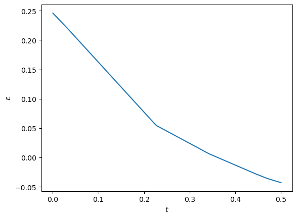
Figure 2: $\epsilon_{\phi}(t)$ trained via (22) on the dataset Figure 4.

We present the pseudocode for training (19) and (22) in Algorithm 1. In practice, we use forward noising dynamics with GM drift (GM+NDSM-CV), as detailed in Section 2.1, where the parameters of GM are obtained from the data via an inexpensive preprocessing step. We note that updating $\epsilon_{\phi}$ according to (22) is expensive, due to the required per-sample gradient computations. Therefore we only update after every $N_{CV}$ SGD updates of $\theta$; in practice we use $N_{CV}=20$, which we find gives good performance while having only a minor impact on computational cost. At the cost of moderately higher variance, one can also simply fix $\epsilon=0$ (i.e., only canceling the singular term) in which case the $\phi$ update step is omitted in Algorithm 1. In Figure 2 we plot the final $\epsilon_{\phi}(t)$ that was obtained after training via (22) on the example from Figure 4 below. We note that the result is well-behaved and remains small but is not identically zero.

4 Low-dimensional examples

In this section we present low-dimensional multi-modal distribution examples which illustrate key aspects of the NDSM-CV method with Gaussian mixture forward dynamics (GM+NDSM-CV); these examples are motivated by clustering in latent space after auto-encoding, as in, e.g., Ding et al. [2019], Li et al. [2023]. We will compare these results with those of linear (OU) forward dynamics and denoising score matching (OU+DSM). Further implementation details can be found in Appendix A.2

In Figures 4-4 we compare standard DSM, Figure 4, with the NDSM-CV methods, both with fixed $\epsilon$ and with $\epsilon_{\phi}(t)$ trained via (22); all methods were trained for 50000 SGD steps. The NDSM-CV methods use GM noising dynamics with $\Delta t=0.001$ in the loss (9). NDSM-CV with $\epsilon=0$ corresponds to a complete cancellation of the term singular that becomes singular as $\Delta t\to 0$, while $\epsilon=1$ corresponds to undoing this cancellation; see the discussion before Theorem 3.1 as well as the proof. This fact explains the discrepancy between Figures 4 and 4, with the former ($\epsilon=1$) showing degraded performance while the latter ($\epsilon=0$) significantly outperforms DSM. This effect is even more apparent when training for fewer SGD steps; see Figure 8 in Appendix B. The best performance is obtained when $\epsilon_{\phi}(t)$ is trained via (22), see Figure 4, both in terms of matching the support of the target distribution as well as having better balance between the modes. Further experiments can be found in Appendix B. In particular, in Figure B-B we show the effect of the perturbation step size $\Delta t$ that enters into the NDSM loss (9).

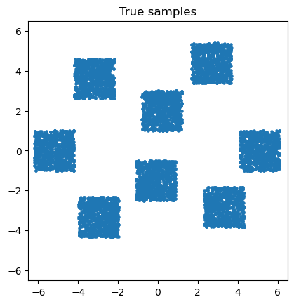
Figure 3(()): True samples

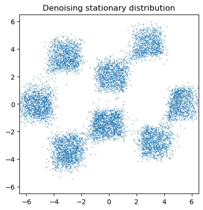
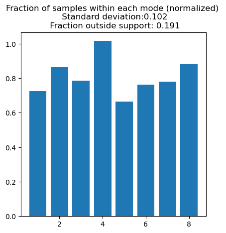
Figure 3(()): OU+DSM

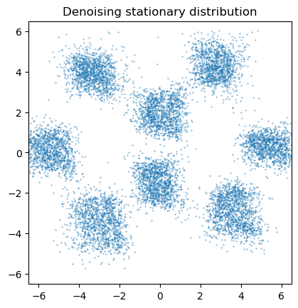
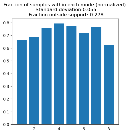
Figure 3(()): GM+NDSM-CV: $\epsilon=1$ (i.e., without control variate)

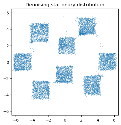
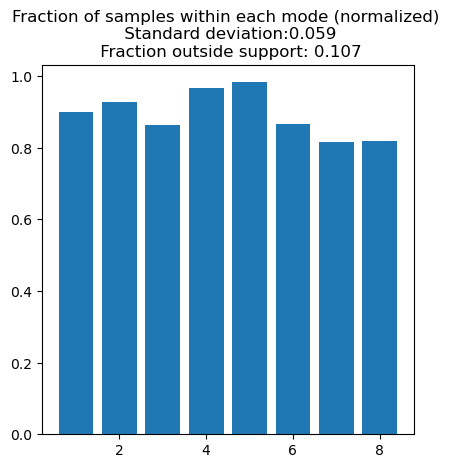
Figure 3(()): GM+NDSM-CV: $\epsilon=0$

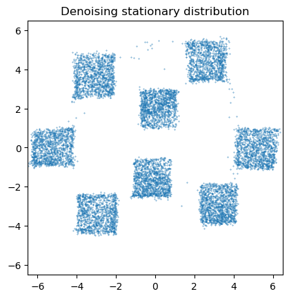
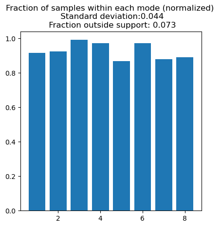
Figure 3(()): GM+NDSM-CV: $\epsilon_{\phi}(t)$ trained via (22)

5 High-dimensional image examples

Finally, we demonstrate the enhanced performance of our proposed GM+NDSM-CV model in learning high-dimensional structured distributions, compared to the benchmark OU+DSM. Specifically, we evaluate their performance using the following two datasets:

(a) MNIST: A collection of 60,000 handwritten digits stored as $28\times 28$ grayscale images [LeCun et al., 1998]. This dataset inherently represents a multi-modal distribution, with each digit class forming at least one mode.

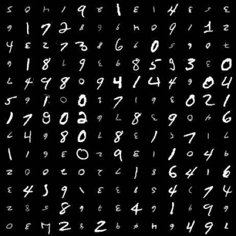
Figure 6: Random samples from the Approx.-$C_{2}$-MNIST dataset. Note that smaller digits are always upside-down, whereas the larger digits (those that are not transformed) remain upright.

(b) Approx.-$C_{2}$-MNIST: This dataset is constructed by randomly rotating MNIST digits by $180^{\circ}$ with a probability of 1/2 and resizing to half-size, creating a distribution that is approximately—but not exactly—invariant under the discrete rotation group $C_{2}$. For a visual illustration of the image samples, refer to Figure 6 in the appendix. It is important to note that the smaller digits are always upside-down, whereas the larger digits (those that are not transformed) remain upright.

A detailed description of the experimental setup and model architecture is provided in Appendix A.3. For the Approx.-$C_{2}$-MNIST dataset, we also consider group-equivariant score models, achieved by symmetrizing a standard score model under the $C_{2}$ group [Lu et al., 2024, Hoogeboom et al., 2022]; such models have shown superior performance over their non-equivariant counterparts in learning distributions that are exactly group invariant. For the benchmark OU+DSM, we mainly use the Variance Preserving (VP) SDE [Sohl-Dickstein et al., 2015, Ho et al., 2020, Song et al., 2020] as the forward noising dynamics.

5.1 MNIST

Table 1: IS and FID on MNIST

Model	IS$\uparrow$	FID$\downarrow$
OU+DSM	6.76	143.3
Our model; $\epsilon=0$	8.82	37.4
Our model; $\epsilon_{\phi}(t)$ trained	8.93	36.1

Table 2: Low data MNIST ($N=14000$)

Model	IS$\uparrow$	FID$\downarrow$
OU+DSM	5.17	470.92
Our model; $\epsilon_{\phi}(t)$ trained	6.89	190.63

A mixture of ten Gaussians fitted to MNIST digits is used as the stationary (prior) distribution for GM-NDSM-CV. For computational efficiency, the covariance matrix of each component is a constant but potentially distinct multiple of the identity matrix. We use a small timestep, $\Delta t=10^{-3}$, to ensure accurate simulation of the forward nonlinear SDE.

The top row of Figure 4 displays random samples generated by different models, and the bottom row shows the class distribution of these samples. The benchmark OU+DSM (Figure 4(a)) exhibits “model collapse,” predominantly generating “easy digits” such as 1 (over 30%) and 7. Our models without or with neural control variate, shown in Figure 4(b) and Figure 4(c) respectively, address this issue by producing more evenly distributed samples across all classes with consistent quality.

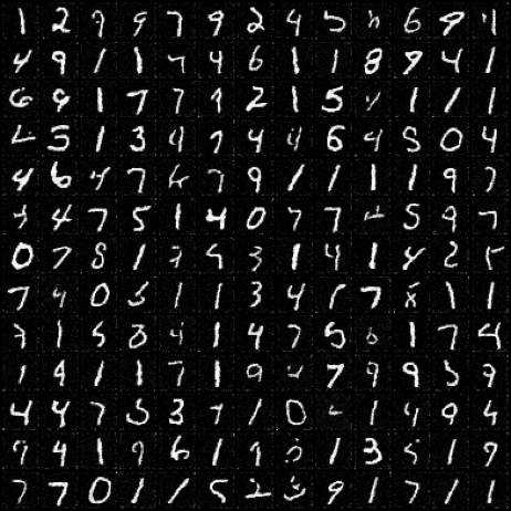
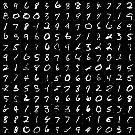
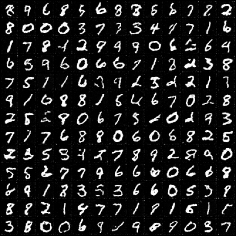
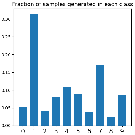
(a) OU+DSM

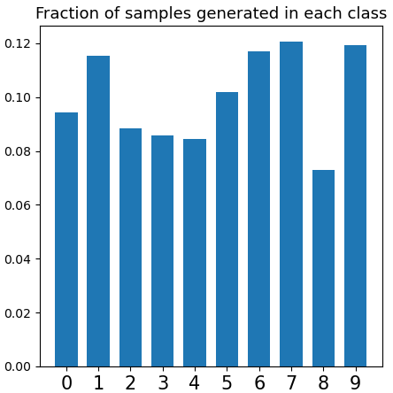
(b) GM+NDSM-CV: $\epsilon=0$

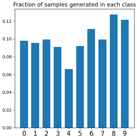
(c) GM+NDSM-CV: $\epsilon_{\phi}(t)$ trained

Figure 4: Top row: random samples generated by different models on the MNIST dataset. Bottom row: the fraction of samples generated in each digit class from 0 to 9.

Table 2 presents the inception score (IS, higher is better) [Salimans et al., 2016] and Fréchet inception distance (FID, lower is better) [Heusel et al., 2017], evaluated using a pre-trained ResNet18 classifier on MNIST. These metrics affirm that our models significantly surpass the benchmark OU+DSM, with the neural control variate model achieving the best results, corroborating the visual evidence in Figure 4. In addition, in Figure 1 we demonstrate that the structure encoded in the GM drift yields an SGM that learns with fewer training samples. We note that for the MNIST examples we have used a smaller NN (see Appendix A.3) than employed by some other studies so as to reduce the computational cost and focus on the effects of nonlinear dynamics and corresponding score matching method.

5.2 Approx.-$C_{2}$-MNIST

Given the approximate $C_{2}$-symmetry, we fit two Gaussians with shared covariance matrices to the dataset as a preprocessing step for GM-NDSM-CV. Figure 5 showcases random samples from various models. Notably, the benchmark OU+DSM, both with (Figure 5(b)) and without (Figure 5(a)) an equivariant score model, consistently exhibits mode collapse, predominantly generating the “easy mode” of small digits. Additionally, the OU+DSM with the equivariant score model introduces another issue by producing “fake samples” such as large-but-upside-down and small-but-upright digits (highlighted in red in Figure 5(b)), indicating that the model erroneously learns from the $C_{2}$-symmetrized version of the underlying distribution. For comparison, see Figure 6 for true samples from this dataset. These issues are effectively addressed by our models (Figures 5(c) and 5(d)), which leverage a flexible design of the stationary distribution and a tailored nonlinear diffusion for the data.

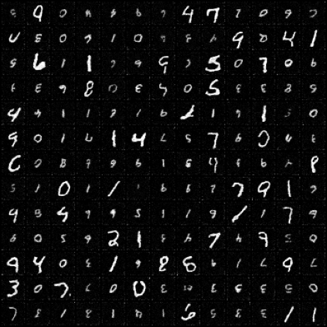
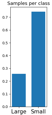
(a) OU+DSM

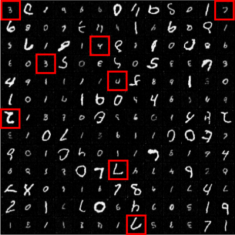
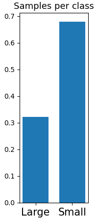
(b) OU+DSM, equivariant score model

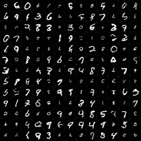
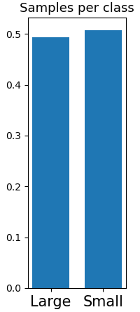
(c) GM+NDSM-CV, $\epsilon=0$

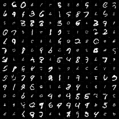
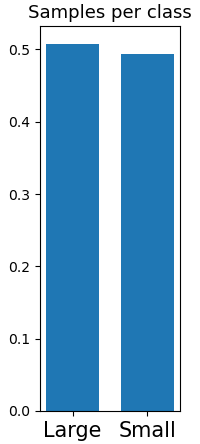
(d) GM+NDSM-CV, $\epsilon_{\phi}(t)$ trained

Figure 5: Approx.-$C_{2}$-MNIST. Problematic “fake samples,” such as large-but-upside-down and small-but-upright digits, are highlighted in panel (b) when using an equivariant score model.

6 Limitations and Conclusions

The NDSM-CV method is a general purpose method for training generative models that allows for the use of nonlinear noising dynamics, thereby incorporating appropriate information on the structure of the data into the dynamics and prior distribution. We have demonstrated that generative models trained using the proposed NDSM-CV method can attain significant improvement in the quality of generative models and allow them to be trained with substantially smaller data sets. These features, although appealing and potentially impactful in practice, could also be used to generate more easily deepfakes for disinformation. We note that there are several limitations associated with the method, as implemented in the code found in the supplemental material. 1) The nonlinear dynamics is currently restricted to encoding structure in the mean and isotropic (i.e., spherical) covariance of a Gaussian mixture model. The theory allows for general nonlinear dynamics, but further work is required to make efficient and effective use of additional structure information. 2) The main theoretical result, Theorem 3.1, involves the cancellation of a mean-zero term that has singular variance as the timestep approaches zero. This is necessary for the nonlinear denoising score matching method to be useful in practice, but it does increase the computational cost of the NDSM objective as compared to the DSM objective. 3) Unlike the case of linear dynamics, which can be sampled at finite times in a single step, the nonlinear forward dynamics must be simulated, e.g., by the EM method. We use several techniques, such as reusing sample paths but with different randomly sampled timesteps, to increase the efficiency, but the necessity of simulating the nonlinear SDE still adds additional computational cost. We anticipate that the method presented here will be more efficient when applied to latent space, as the cost of simulating a high-dimensional nonlinear diffusion is less significant. This is a direction for future work.

Appendix A Implementation details

Here we present implementation details for the examples from Sections 4 and 5. See also the full code in the supplemental materials.

A.1 Pseudocode

The pseudocode for the NDSM-CV method was presented in the main text; see Algorithm 1. Here in Algorithms 2 and 3 we present the pseudocode for the noising and denoising dynamics respectively, where the SDEs are simulated using the EM method. The noising dynamics start in the data distribution, $\pi$, while the denoising dynamics start in the Gaussian mixture prior $\eta_{*}$ (2), which is the invariant distribution for the noising dynamics. The parameters for $\eta_{*}$ are obtained by fitting a Gaussian mixture model to (a portion of) the training data.

Algorithm 2 Forward Noising Dynamics (given the data distribution $\pi$)

1:Sample $y_{1},...,y_{B}$ from $\pi$

2:$y_{j,0}=y_{j}$

3:for $n=0,...,n_{f}-1$ do

4:     Sample $Z_{n+1}\sim N(0,I)$

5:     $y_{i,n+1}=y_{i,n}-\nabla V(y_{i,n})\Delta t_{n}+\sqrt{2\Delta t_{n}}Z_{n+1}$

6:end for

Algorithm 3 Denoising Dynamics (given the trained score model $s_{\theta}$)

1:Sample $x_{1},...,x_{B}$ from $\eta_{*}$    (see Eq. 2)

2:$y_{j,0}=y_{j}$

3:for $n=0,...,n_{f}-1$ do

4:     Sample $Z_{n+1}\sim N(0,I)$

5:     $x_{i,n+1}=x_{i,n}+(\nabla V(y_{i,n})+2s_{\theta}(x_{i,n},T-t_{n}))\Delta t_{n}+\sqrt{2\Delta t_{n}}Z_{n+1}$

6:end for

A.2 Low dimensional examples

The examples in Section 4 used a score model with 7 fully connected hidden layers, each with 32 nodes, and GELU activations. The control-variate method uses $\epsilon_{\phi}$ that has 3 fully connected hidden layers, each with 10 nodes, and ReLU activations. Both are trained with a learning rate to $10^{-3}$ on 10000 training samples. The losses all use a minibatch size of 250. In the case of DSM they consist of 250 samples from the data distribution, evolved under the linear dynamics up to a random time. In the case of NDSM-CV, they consist of 50 samples evolved under the nonlinear dynamics, with each trajectory samples at 5 random times along the trajectory. The results in Figures 4-4 were obtained after training for 10000 SGD steps while those in B-B were trained for 50000 SGD steps.

A.3 Image examples

The examples in Section 5 use the U-net [Ronneberger et al., 2015] architecture as the backbone of the score network $s_{\theta}(y,t)$. More specifically, the encoder part of the score model comprises four blocks with decreasing spatial resolution, each containing a $3\times 3$ convolution layer, group normalization layer, and a “swish” activation function [Ramachandran et al., 2017]. Time information is incorporated via Gaussian random features [Tancik et al., 2020] and propagated through fully connected layers in each encoder block. The decoder, defined similarly with increasing spatial resolution, includes skip connections from the encoding to the decoding path.

For the benchmark OU+DSM, we consider mainly the Variance Preserving (VP) SDE [Sohl-Dickstein et al., 2015, Ho et al., 2020, Song et al., 2020] as the forward diffusion process:

$$dY(t)=-\frac{1}{2}\beta(t)ydt+\sqrt{\beta(t)}dW(t),$$ (23)

where $\beta(t)$ is a linear function on $[0,T]$, with $\beta(0)=0.1$ and $\beta(T)=20$. The terminal time is set to $T=1$. For NDSM-CV, we use Langevin dynamics with the preprocessed Gaussian Mixture as the stationary distribution for the forward diffusion process, with the terminal time set to $T=2$.

All models are trained using the Adam optimizer with a batch size of 64 for 100 epochs on a Linux machine equipped with a GeForce RTX 3090 GPU.

Appendix B Additional experiments

In Figure B-B we show the effect of the perturbation stepsize $\Delta t$ that enters into the NDSM loss (9); we note that the perturbation timestep, $\Delta t$, which is used for the samples that enter into the loss can be chosen independently from the timesteps that do not enter into the loss; the latter is fixed at $0.00998$ in this example. We compare the results with DSM, Figure B, which does not have an analogous $\Delta t$ parameter. We observe that a smaller $\Delta t$ is more capable of learning distributions with (approximate) lower dimensional support. The GM dynamics also lead to samples that are more evenly distributed amongst the modes, similar to what was seen in Figures 4-4.

In Figure 8 we show the example from Figures 4-4, but here trained for 10000 SGD steps as opposed to 50000. Again we see that the NDSM-CV method achieves better performance than DSM with the same number of SGD steps, and has better balance between the modes. Comparing Figures 8 and 8 we see the important of canceling the singular term in the objective; the former ($\epsilon=0$) completely cancels this term while the latter ($\epsilon=1$) leaves it in its entirety and thus has significantly degraded performance. The best performance, shown in Figure 8, is obtained when $\epsilon_{\phi}(t)$ is optimized to minimize the MSE, as in (22).

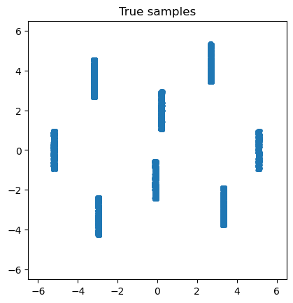
Figure 7(()): True samples

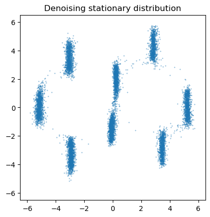
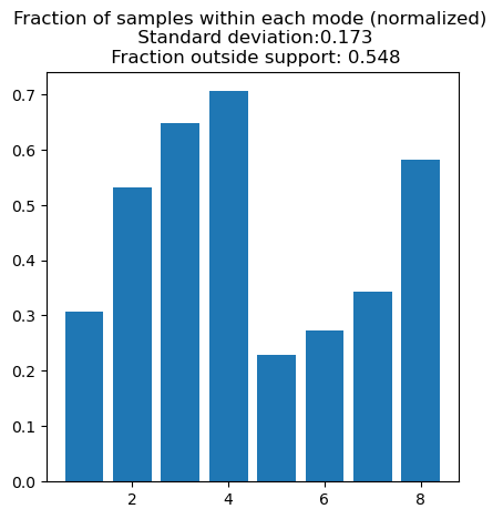
Figure 7(()): OU+DSM

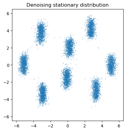
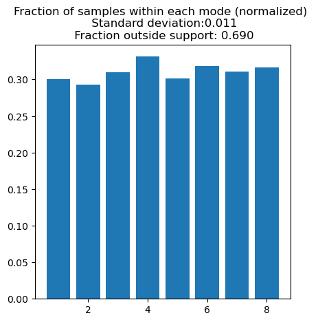
Figure 7(()): GM+NDSM-CV: $\Delta t=0.05$

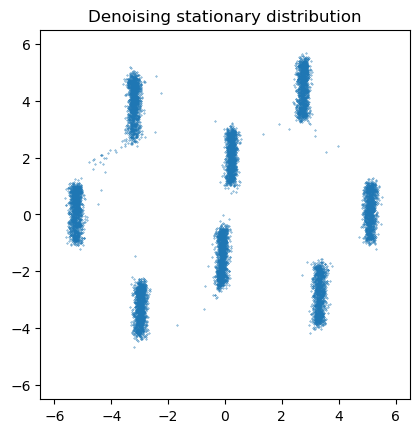
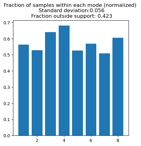
Figure 7(()): GM+NDSM-CV: $\Delta t=0.01$

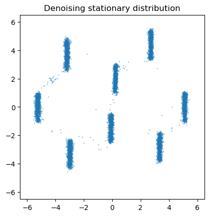
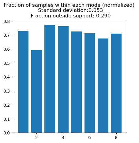
Figure 7(()): GM+NDSM-CV: $\Delta t=0.005$

Figure 8(()): True samples

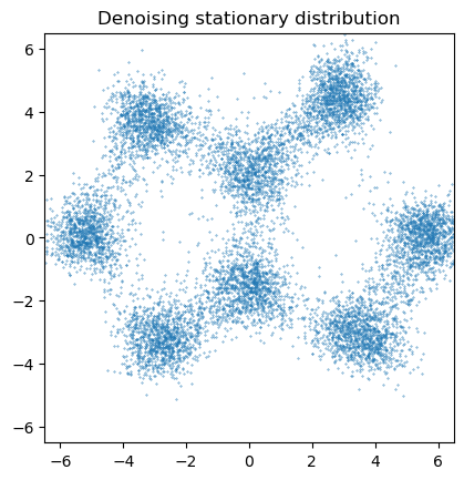
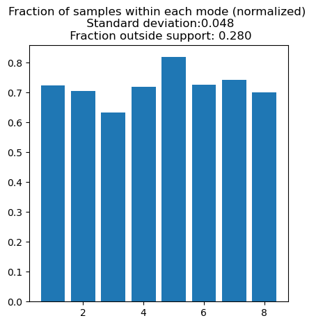
Figure 8(()): OU+DSM

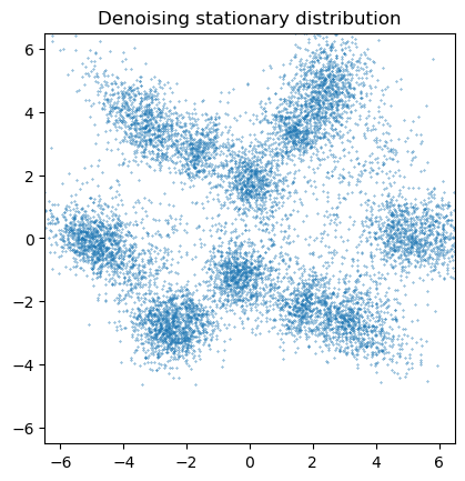
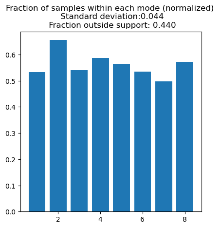
Figure 8(()): GM+NDSM-CV: $\epsilon=1$ (i.e., without control variate)

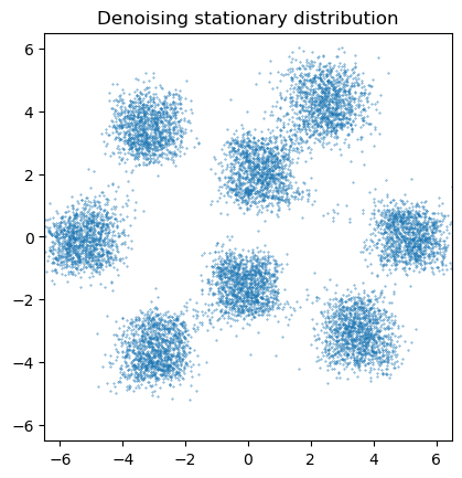
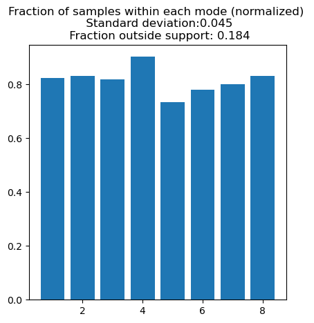
Figure 8(()): GM+NDSM-CV: $\epsilon=0$

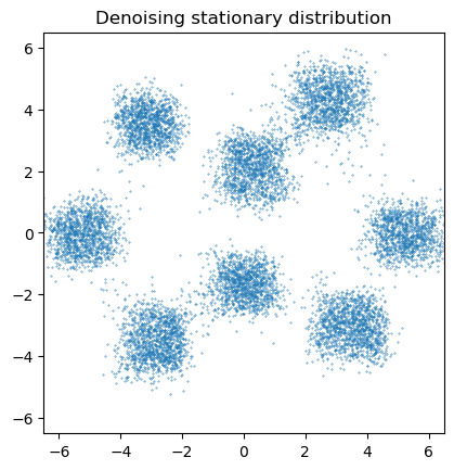
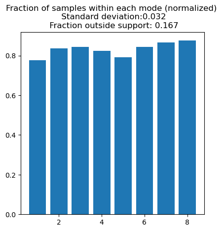
Figure 8(()): GM+NDSM-CV: $\epsilon_{\phi}(t)$ trained via (22)

Figure 8: The same example as in Figures 4-4, but trained for 10000 SGD steps.

References

- Asmussen and Glynn [2007] S. Asmussen and P. W. Glynn. Stochastic simulation: algorithms and analysis, volume 57. Springer, 2007.
- Berner et al. [2022] J. Berner, L. Richter, and K. Ullrich. An optimal control perspective on diffusion-based generative modeling. In NeurIPS 2022 Workshop on Score-Based Methods, 2022.
- Collet et al. [2013] P. Collet, S. Martínez, J. San Martín, et al. Quasi-stationary distributions: Markov chains, diffusions and dynamical systems, volume 1. Springer, 2013.
- Ding et al. [2019] X. Ding, Z. Zou, and C. L. Brooks III. Deciphering protein evolution and fitness landscapes with latent space models. Nature communications, 10(1):5644, 2019.
- Dockhorn et al. [2021] T. Dockhorn, A. Vahdat, and K. Kreis. Score-based generative modeling with critically-damped langevin diffusion. arXiv preprint arXiv:2112.07068, 2021.
- Goodfellow et al. [2014] I. Goodfellow, J. Pouget-Abadie, M. Mirza, B. Xu, D. Warde-Farley, S. Ozair, A. Courville, and Y. Bengio. Generative adversarial nets. Advances in neural information processing systems, 27, 2014.
- Grathwohl et al. [2018] W. Grathwohl, R. T. Chen, J. Bettencourt, I. Sutskever, and D. Duvenaud. FFJORD: Free-form continuous dynamics for scalable reversible generative models. arXiv preprint arXiv:1810.01367, 2018.
- Heusel et al. [2017] M. Heusel, H. Ramsauer, T. Unterthiner, B. Nessler, and S. Hochreiter. Gans trained by a two time-scale update rule converge to a local nash equilibrium. In I. Guyon, U. V. Luxburg, S. Bengio, H. Wallach, R. Fergus, S. Vishwanathan, and R. Garnett, editors, Advances in Neural Information Processing Systems, volume 30. Curran Associates, Inc., 2017. URL https://proceedings.neurips.cc/paper_files/paper/2017/file/8a1d694707eb0fefe65871369074926d-Paper.pdf.
- Ho et al. [2020] J. Ho, A. Jain, and P. Abbeel. Denoising diffusion probabilistic models. Advances in neural information processing systems, 33:6840–6851, 2020.
- Hoogeboom et al. [2022] E. Hoogeboom, V. G. Satorras, C. Vignac, and M. Welling. Equivariant diffusion for molecule generation in 3d. In International conference on machine learning, pages 8867–8887. PMLR, 2022.
- LeCun et al. [1998] Y. LeCun, L. Bottou, Y. Bengio, and P. Haffner. Gradient-based learning applied to document recognition. Proceedings of the IEEE, 86(11):2278–2324, 1998.
- Lelièvre et al. [2022] T. Lelièvre, M. Ramil, and J. Reygner. Quasi-stationary distribution for the langevin process in cylindrical domains, part i: existence, uniqueness and long-time convergence. Stochastic Processes and their Applications, 144:173–201, 2022.
- Li et al. [2023] Y. Li, Y. Yao, Y. Xia, and M. Tang. Searching for protein variants with desired properties using deep generative models. BMC bioinformatics, 24(1):297, 2023.
- Lu et al. [2024] H. Lu, S. Szabados, and Y. Yu. Structure preserving diffusion models. arXiv preprint arXiv:2402.19369, 2024.
- Pavliotis [2014] G. A. Pavliotis. Stochastic processes and applications. Texts in Applied Mathematics, 60, 2014.
- Ramachandran et al. [2017] P. Ramachandran, B. Zoph, and Q. V. Le. Searching for activation functions. arXiv preprint arXiv:1710.05941, 2017.
- Rombach et al. [2022] R. Rombach, A. Blattmann, D. Lorenz, P. Esser, and B. Ommer. High-resolution image synthesis with latent diffusion models. In Proceedings of the IEEE/CVF conference on computer vision and pattern recognition, pages 10684–10695, 2022.
- Ronneberger et al. [2015] O. Ronneberger, P. Fischer, and T. Brox. U-net: Convolutional networks for biomedical image segmentation. In Medical image computing and computer-assisted intervention–MICCAI 2015: 18th international conference, Munich, Germany, October 5-9, 2015, proceedings, part III 18, pages 234–241. Springer, 2015.
- Rubinstein [2009] R. Rubinstein. Simulation and the Monte Carlo Method. Wiley Series in Probability and Statistics. Wiley, 2009. ISBN 9780470317228. URL https://books.google.com/books?id=PUpdaQZsCK0C.
- Salimans et al. [2016] T. Salimans, I. Goodfellow, W. Zaremba, V. Cheung, A. Radford, and X. Chen. Improved techniques for training gans. Advances in neural information processing systems, 29, 2016.
- Sohl-Dickstein et al. [2015] J. Sohl-Dickstein, E. Weiss, N. Maheswaranathan, and S. Ganguli. Deep unsupervised learning using nonequilibrium thermodynamics. In International conference on machine learning, pages 2256–2265. PMLR, 2015.
- Song et al. [2020] Y. Song, J. Sohl-Dicks tein, D. P. Kingma, A. Kumar, S. Ermon, and B. Poole. Score-based generative modeling through stochastic differential equations. arXiv preprint arXiv:2011.13456, 2020.
- Tancik et al. [2020] M. Tancik, P. Srinivasan, B. Mildenhall, S. Fridovich-Keil, N. Raghavan, U. Singhal, R. Ramamoorthi, J. Barron, and R. Ng. Fourier features let networks learn high frequency functions in low dimensional domains. Advances in neural information processing systems, 33:7537–7547, 2020.
- Vahdat et al. [2021] A. Vahdat, K. Kreis, and J. Kautz. Score-based generative modeling in latent space. Advances in Neural Information Processing Systems, 34:11287–11302, 2021.
- Vincent [2011] P. Vincent. A connection between score matching and denoising autoencoders. Neural computation, 23(7):1661–1674, 2011.
- Xiao et al. [2021] Z. Xiao, K. Kreis, and A. Vahdat. Tackling the generative learning trilemma with denoising diffusion GANs. arXiv preprint arXiv:2112.07804, 2021.
- Zhang and Katsoulakis [2023] B. J. Zhang and M. A. Katsoulakis. A mean-field games laboratory for generative modeling. arXiv preprint arXiv:2304.13534, 2023.
- Zhang et al. [2024] B. J. Zhang, S. Liu, W. Li, M. A. Katsoulakis, and S. J. Osher. Wasserstein proximal operators describe score-based generative models and resolve memorization. arXiv preprint arXiv:2402.06162, 2024.