Trajectory-Based Multi-Objective Hyperparameter Optimization for Model Retraining

Abstract

Training machine learning models inherently involves a resource-intensive and noisy iterative learning procedure that allows epoch-wise monitoring of the model performance. However, in multi-objective hyperparameter optimization scenarios, the insights gained from the iterative learning procedure typically remain underutilized. We notice that tracking the model performance across multiple epochs under a hyperparameter setting creates a trajectory in the objective space and that trade-offs along the trajectories are often overlooked despite their potential to offer valuable insights to decision-making for model retraining. Therefore, in this study, we propose to enhance the multi-objective hyperparameter optimization problem by having training epochs as an additional decision variable to incorporate trajectory information. Correspondingly, we present a novel trajectory-based multi-objective Bayesian optimization algorithm characterized by two features: 1) an acquisition function that captures the improvement made by the predictive trajectory of any hyperparameter setting and 2) a multi-objective early stopping mechanism that determines when to terminate the trajectory to maximize epoch efficiency. Numerical experiments on diverse synthetic simulations and hyperparameter tuning benchmarks indicate that our algorithm outperforms the state-of-the-art multi-objective optimizers in both locating better trade-offs and tuning efficiency.

1 Introduction

With the expanding complexity of machine learning (ML) models, there is a significant surge in the demand for Hyperparameter Optimization (HPO). This surge is not only in pursuit of model prediction accuracy but also for ensuring the computational efficiency and robustness of models in real-world scenarios, which leads to the Multi-Objective Hyperparameter Optimization (MOHPO) [12, 21, 28]. Addressing HPO has long been challenging as it involves resource-intensive model training that prevents optimizers from exhaustively exploring the hyperparameter space. In this context, Bayesian Optimization (BO) has become increasingly popular [4, 36]. This approach builds a probabilistic surrogate model, e.g., Gaussian Process (GP) [33], for the objective and samples a new solution by maximizing an acquisition function formulated by the prediction and uncertainty of the surrogate model. Due to the sample efficiency of BO, many research works have extended it in different ways to Multi-Objective BO (MOBO) and successfully applied to solve MOHPO [1, 8, 9].

Nevertheless, conventional BO methods require observing the model performance that is fully trained after a maximum number of epochs, which could potentially lead to a waste of computational resources if early indications suggest sub-optimal performance. In general, the training behind many ML models is an iterative learning procedure where a gradient-based optimizer updates the model epoch by epoch. This procedure allows users to delineate a learning curve for any hyperparameter setting by epoch-wisely monitoring the intermediate model performance (see Figure 1(A) and (B)), benefiting from which the literature has presented a set of epoch-efficient single-objective BO methods [38, 7, 29, 3] to avoid computational waste. Unfortunately, to the best of our knowledge, there remains a gap in multi-objective research that fully accounts for iterative learning procedures.

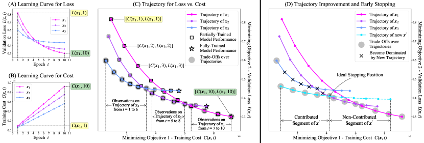
Figure 1: (A) and (B): Learning curves of three hyperparameter settings $\bm{x}_{1}$, $\bm{x}_{2}$, and $\bm{x}_{3}\in\mathbb{R}^{d}$; (C): Trajectories of $\bm{x}_{1}$, $\bm{x}_{2}$, and $\bm{x}_{3}$ and trade-offs over their model performances; (D) Trajectory-based improvement and early stopping when a new $\bm{x}^{\prime}\in\mathbb{R}^{d}$ is sampled. $L(\bm{x},t)$ (or $C(\bm{x},t)$) denotes the validation loss (or cost) of training with $\bm{x}\in\mathbb{R}^{d}$ for $t$ epochs. The maximum number of epochs is 10.

Considering MOHPO with iterative learning procedures motivates the critical question of whether a trade-off that achieves the best model performance under a fixed training cost exists when training with fewer epochs than the maximum allowed. Figure 1(C) depicts such a bi-objective scenario, where we extend the concept of the learning curve by introducing “trajectory” to describe the iterative training procedure. For instance, the trajectory of a $d$-dimensional hyperparameter setting $\bm{x}_{1}$ consists of its model performances (training cost and validation loss) observed from epoch $t=1$ to $10$. The emergence of trajectories reveals the limitation of traditional MOHPO in that it focuses only on fully-trained model performances ($t=10$) and ignores a large amount of partially-trained model performances ($t<10$) that can also contribute to trade-offs. Nevertheless, these trade-offs offer valuable insights for decision-making in scenarios where ML models are periodically retrained on similar datasets with similar performance and need rapid deployment, such as recurrent data analyst jobs in the cloud [5, 27] and data drift detection in self-adaptive systems [25, 6]. To avoid repetitive and costly tuning in these cases, it is a common practice to use the same hyperparameter setting for every retraining [44, 21], which makes it important to understand at the initial stage how many epochs to retrain to strike the desired balance between objectives. Consequently, in this study, we propose to tune the hyperparameter setting together with the number of training epochs and formulate an Enhanced MOHPO (i.e., EMOHPO).

To effectively solve EMOHPO, it is necessary to develop a new MOBO method capable of integrating the information drawn from trajectories into sequential sampling. Given that a trajectory may contribute more than one trade-off (illustrated in Figure 1(C)), assessing the quality of a hyperparameter setting in EMOHPO requires a comprehensive consideration of its entire trajectory. Existing multi-objective acquisition functions tend to favor hyperparameter settings with superior model performance at a single position, which potentially leads to trajectories with limited trade-offs. Furthermore, similar to single-objective scenarios, as an iterative learning procedure proceeds, we can epoch-wisely update predictions for the unobserved segment of the trajectory and decide on termination to improve algorithm efficiency. However, it is crucial to guarantee that such an early stopping mechanism does not compromise the optimization outcomes. In the context of EMOHPO, this implies that only after observing as many trade-offs along the trajectory as possible can the iterative learning procedure be stopped.

Contributions: (1) For the first time we formulate EMOHPO, a variant of MOHPO enhanced by the trajectory information, to account for the evolution of model performance across epochs and hence uncover trade-offs that are often overlooked in conventional MOHPO studies. (2) We introduce a novel trajectory-based MOBO method for EMOHPO. The proposed method samples the next hyperparameter setting based on the quality of its anticipated trajectory and subsequently determines when to terminate the trajectory to maximize epoch efficiency. (3) Through comprehensive experiments on synthetic simulations and machine learning benchmarks, we demonstrate the effectiveness and efficiency of our method in identifying trade-offs while conserving computational resources.

2 Enhanced Multi-Objective Hyperparameter Optimization Problem

Throughout the paper, we consider the sequential minimization of an Enhanced Multi-Objective Hyperparameter Optimization problem (EMOHPO) in the following form:

$$\min_{(\bm{x},t)\in\mathbb{X}\times\mathbb{T}}\bm{f}(\bm{x},t)=\left[f_{1}(\bm{x},t),\dots,f_{k}(\bm{x},t)\right],$$ (1)

where $\bm{f}$ comprises $k$ objective functions, each of which represents a different performance measure of an ML model, e.g., validation loss and training cost. Each $\bm{x}$ is a $d$-dimensional hyperparameter setting within a compact set $\mathbb{X}\subset\mathbb{R}^{d}$. We further consider an iterative learning procedure, where, with any feasible hyperparameter setting $\bm{x}$, we can train the ML model for any epoch $t\in\mathbb{T}=\{1,\dots,t_{max}\}$ and observe the intermediate but noisy performance $\bm{y}(\bm{x},t)=\left[y_{1}(\bm{x},t),\dots,y_{k}(\bm{x},k)\right]$ where $y_{i}(\bm{x},t)=f_{i}(\bm{x},t)+\varepsilon_{i}$ and $\varepsilon_{i}\sim\mathcal{N}(0,\sigma_{i}^{2})$ with variance $\sigma_{i}^{2}$ for any $i\in\{1,\dots,k\}$. Let $\bm{z}=(\bm{x},t)$ denote any feasible query pair and $\mathbb{Z}=\mathbb{X}\times\mathbb{T}$ the overall feasible domain. As per Definitions 1 and 2 below, solving the EMOHPO in (1) is equivalent to locating a set of trade-offs that approximate the Pareto-optimal set and front as accurately as possible. When making the final decision, for example, among the trade-offs of EMOHPO shown in Figure 1(C), one can easily select the best pair $(\bm{x},t)$ - referring to training the ML model with hyperparameter setting $\bm{x}$ for $t$ epochs - to achieve the desired level of validation loss within a feasible time budget.

Definition 1.

A solution $\bm{f}(\bm{z})$ dominates another solution $\bm{f}(\bm{z}^{\prime})$, denoted by $\bm{f}(\bm{z})\prec\bm{f}(\bm{z}^{\prime})$, if and only if (1) $f_{i}(\bm{z})\leq f_{i}(\bm{z}^{\prime})$ for all $i\in\{1,\dots,k\}$ and (2) $f_{j}(\bm{z})<f_{j}(\bm{z}^{\prime})$ for some $j\in\{1,\dots,k\}$.

Definition 2.

The Pareto-optimal set $Z^{*}$ is composed of query pair $\bm{z}$ whose $\bm{f}(\bm{z})$ is not dominated by $\bm{f}(\bm{z}^{\prime})$ of any other $\bm{z^{\prime}}\in\mathbb{Z}$, i.e., $Z^{*}=\{\bm{z}\mid\bm{z}\in\mathbb{Z},\nexists\bm{z}^{\prime}\in\mathbb{Z},\bm{f}(\bm{z}^{\prime})\prec\bm{f}(\bm{z})\}$. The corresponding set of solutions $F^{*}=\{\bm{f}(\bm{z})\mid\bm{z}\in Z^{*}\}$ is referred to as Pareto-optimal front.

In the context of iterative learning, each objective function $f_{i}(\bm{x},\cdot)$, for $i\in\{1,\dots,k\}$, can be treated as a learning curve associated with hyperparameter setting $\bm{x}$. However, a learning curve only enables the analysis of one performance measure at a time. To holistically analyze multiple performance measures, we introduce the concept of trajectory and define it as the collection of all observable model performances during the training with hyperparameter setting $\bm{x}$, i.e., $Trj(\bm{x}):=\{\bm{f}(\bm{x},t)\}_{t=1}^{t_{max}}=\{\left[f_{1}(\bm{x},t),\dots f_{k}(\bm{x},t)\right]\}_{t=1}^{t_{max}}$. Inherently, a trajectory encapsulates the information provided by multiple learning curves.

As demonstrated in Section 1, EMOHPO is an enhancement of the standard MOHPO with the information provided by trajectories. More specifically, compared to (1), MOHPO restricts its identification of trade-offs among the fully-trained model performances and is expressed as,

$$\min_{\bm{x}\in\mathbb{X}}\bm{f}(\bm{x},t_{max})=\left[f_{1}(\bm{x},t_{max}),\dots,f_{k}(\bm{x},t_{max})\right],$$ (2)

where the second input $t_{max}$ is a fixed constant and is always assumed to be implicit in earlier studies’ formulations [23, 8, 9]. Taking the second input as an explicit variable $t$ significantly distinguishes EMOHPO from standard MOHPO in two aspects: (I) EMOHPO allows an optimizer to collect observations from $\bm{f}(\bm{x},1)$ to $\bm{f}(\bm{x},t)$ when querying at $(\bm{x},t)$ because the value of $\bm{f}(\bm{x},t^{\prime})$ is observed before $\bm{f}(\bm{x},t)$ for any $t^{\prime}<t$. This feature necessitates the design of a more sample-efficient strategy, which aims to avoid repeatedly visiting the same hyperparameter setting across different epoch numbers. (II) EMOHPO broadens the optimization domain from $\mathbb{X}\times\{t_{max}\}$ to $\mathbb{X}\times\mathbb{T}$ and accounts for all observations on the trajectories. As a consequence, the Pareto-optimal front of EMOHPO is superior to or at least equivalent to that of MOHPO because the former additionally captures trade-offs that may emerge during iterative learning (see Figure 1(C)).

3 Related Work in Bayesian Optimization

Bayesian Optimization for Iterative Learning: By appropriately characterizing the learning curve, epoch-efficient BO aims to predict the fully-trained model performance based on a partially observed learning curve to avoid ineffective epochs of training. Freeze-Thaw BO [38] introduces GP with an exponential decaying kernel to model the validation loss over time and allows the training to be paused and later resumed under hyperparameter settings that show promise. BOHB [14], a BO extension of HyperBand [24], allocates training epochs through random sampling and utilizes successive halving to eliminate suboptimal hyperparameter settings. Instead of dynamically allocating computational budget among hyperparameter settings, BO-BOS [7] combines BO with Bayesian optimal stopping to early stop the training with a hyperparameter setting predicted to yield poor model performance. Similarly, both BOIL [29] and BAPI [3] incorporate strategies for early stopping with a particular focus on considering the learning curve of the training cost. BOIL integrates the cost into the acquisition function to prioritize cost-effective ML training procedures, whereas BAPI imposes a fixed total budget over cost. Unfortunately, there has been no epoch-efficient BO designed for MOHPO or EMOHPO.

Multi-Objective Bayesian Optimization: Many MOBO methods have been developed for multi-objective HPO by extending the vanilla BO framework. These methods generally build a surrogate model for each objective to minimize the necessity of actual resource-intensive objective evaluations and they differ in the implementation of acquisition function. A straightforward approach is to convert a multiple-objective problem into a single-objective problem through techniques like random scalarization, which allows a direct application of standard acquisition functions. For example, ParEGO [23] and TS-TCH [30] respectively apply Expected Improvement (EI) [18] and Thompson Sampling (TS) [40]. However, this approach often encounters limitations in adequately exploring the Pareto-optimal front. Therefore, acquisition functions biased towards the Pareto-optimal front, such as Expected Hypervolume Improvement (EHVI) [13], have been designed. Despite the effectiveness and popularity of EHVI, its computational intensity presents a significant challenge in the development of BO methods [17]. More recently, $q$EHVI [8] and $q$NEHVI [9] have extended EHVI for parallel multi-point selection and batch optimization through Monte Carlo (MC) integration [13] and they have demonstrated notable empirical performance. Alternatives to EHVI can be found in [16, 1, 37, 45].

Multi-Fidelity Bayesian Optimization: Multi-fidelity BO has a rich research history [19, 20, 35, 39] and it facilitates the optimization of fully-trained model performance by utilizing its low-fidelity approximations which can be obtained either by using a partial training dataset or by limiting the number of training epochs. Although multi-fidelity BO shares similarities with epoch-efficient BO, it predetermines the fidelity level before initiating the iterative learning procedure and therefore ignores the observations during the procedure. For example, FABOLAS [22] considers the data subset size as the fidelity level and jointly selects the hyperparameter setting and the data subset for model training. BOCA [20] expands the discrete fidelity space to continuous for a more general problem setting. Multi-fidelity MOBO has also been studied in the literature [2]; however, it cannot be applied to solving EMOHPO because the fidelity level is no longer an additional degree of freedom in (4), which makes low-fidelity approximations not available.

4 Gaussian Process for Trajectory Prediction

Assume a black-box function $f$ is sampled from a GP defined by a constant zero mean function and a kernel function $K(\bm{z},\bm{z}^{\prime})$. According to GP theory, the prior distribution over any finite set of $n$ inputs $Z=\{\bm{z}_{i}\}_{i=1}^{n}$ is a multivariate Gaussian distribution,

$$f(Z)\sim\mathcal{N}(\bm{0},K(Z,Z)),$$

where matrix $K(Z,Z)\in\mathbb{R}^{n\times n}$ with $\left[K(Z,Z)\right]_{i,j}=K(\bm{z}_{i},\bm{z}_{j})$. Conditioning on the corresponding observations $Y=\{y_{i}\}_{i=1}^{n}$ at $Z$, the posterior predictive distribution at any input $\bm{z}\in\mathbb{Z}$ is also a Gaussian distribution given by

$$f(\bm{z})\mid Z,Y\sim\mathcal{N}\left(\mu(\bm{z}),\Sigma(\bm{z})\right),$$ (3)

with

$$\mu(\bm{z}) =K(\bm{z},Z)\left[K(Z,Z)+\sigma^{2}I\right]^{-1}Y,$$

$$\Sigma(\bm{z}) =K(\bm{z},\bm{z})-K(\bm{z},Z)\left[K(Z,Z)+\sigma^{2}I\right]^{-1}K(Z,\bm{z}),$$

where $K(\bm{z},Z)=K(Z,\bm{z})^{T}\in\mathbb{R}^{n}$ with $\left[K(\bm{z},Z)\right]_{i}=K(\bm{z},\bm{z}_{i})$. Refer to [33] for a comprehensive review of GPs. In each iteration of the vanilla BO method, a new input $\bm{z}^{\prime}\in\mathbb{Z}$ is selected by optimizing an acquisition function derived from the predictive mean $\mu$ and uncertainty $\Sigma$. Upon observing $y^{\prime}$ at $\bm{z}^{\prime}$, BO advances to the next iteration with the updated input and observation sets $Z=Z\cup\{\bm{z}^{\prime}\}$ and $Y=Y\cup\{y^{\prime}\}$.

As each input $\bm{z}=(\bm{x},t)$, we define the kernel function $K\left((\bm{x},t),(\bm{x}^{\prime},t^{\prime})\right)$ as the product of a standard kernel $K(\bm{x},\bm{x}^{\prime})$ over hyperparameter setting and a temporal kernel $K(t,t^{\prime})$ over epochs, with the latter capturing relationships across different epochs for a fixed hyperparameter setting. For instance, Swersky et al. [38] proposed an exponential decaying kernel to account for the validation loss that exponentially decreases over $t$. Belakaria et al. [3] used a linear kernel when modeling learning curves related to training costs. Given that learning curves for different performance measures may exhibit different characteristics, in this study we employ specific temporal kernels if their behavior is known a priori. By fitting a GP model for each objective function $f_{i}$, $i\in\{1,\dots,k\}$, we can predict the trajectory of any hyperparameter setting $\bm{x}$ and further improve the accuracy of its trajectory prediction by continuously monitoring the changes in model performance during iterative learning.

5 Trajectory-Based Bayesian Optimization Approach

Now we introduce an epoch-efficient algorithm named Trajectory-based Multi-Objective Bayesian Optimization (TMOBO) for solving the EMOHPO as defined in (1). This algorithm is particularly designed to efficiently navigate the trade-off model performances across multiple epochs by leveraging the insights obtained from trajectories. At its core, TMOBO features a trajectory-based acquisition function to sample hyperparameter settings and a trajectory-based early stopping mechanism to determine the number of epochs to train with each hyperparameter setting. The pseudo-code of TMOBO is presented in Algorithm 1.

Algorithm 1 Framework of TMOBO

Input: Initial sets of inputs $Z$ and observations $Y$, and initial Pareto-optimal front $F$ identified from $Y$.

1:while the computational budget has not been exceeded do

2:     Fit $k$ GP models with $\bm{\mu}$ and $\bm{\Sigma}$ based on sets $Z$ and $Y$. $\triangleright$ refer to Section 4

3:     Sample a new $\bm{x}^{\prime}$ by maximizing the TEHVI acquisition function. $\triangleright$ refer to Section 5.1

4:     Initialize $Z^{\prime}\leftarrow\emptyset$ and $Y^{\prime}\leftarrow\emptyset$.

5:     for $t^{\prime}=1$ to $t_{\max}$ do

6:         Continue model training for the $t^{\prime}$-th epoch to obtain observation $\bm{y}(\bm{x}^{\prime},t^{\prime})$.

7:         Let $Z^{\prime}\leftarrow Z^{\prime}\cup\{(\bm{x}^{\prime},t^{\prime})\}$ and $Y^{\prime}\leftarrow Y^{\prime}\cup\{\bm{y}(\bm{x}^{\prime},t^{\prime})\}$ and update front $F$.

8:         Fit $k$ GP models with $\bm{\mu}$ and $\bm{\Sigma}$ based on sets $Z\cup Z^{\prime}$ and $Y\cup Y^{\prime}$.

9:         if EarlyStopping$(\bm{x}^{\prime},t^{\prime},\bm{\mu},\bm{\Sigma},F)$ is triggered then $\triangleright$ refer to Section 5.2

10:              Break;

11:         end if

12:     end for

13:     Augment $Z^{\prime}$ and $Y^{\prime}$ into $Z$ and $Y$ respectively. $\triangleright$ refer to Section 5.2

14:end while

We initiate the algorithm by generating a set of uniformly distributed hyperparameter settings $X=\{\bm{x}_{i}\}_{i=1}^{n_{0}}$. The training datasets, including the set of query pairs $Z$ and the set of noisy multi-objective observations $Y$, are then obtained by training the ML model with each $\bm{x}\in X$ for up to $t_{max}$ epochs. Due to the unavailability of noise-free objective values, we consider the front $F$ of the noisy observations in $Y$ as an approximate representation of the Pareto-optimal front, which is continuously updated with each new observation.

Each iteration of TMOBO is centered around a two-step sampling strategy where a hyperparameter setting $\bm{x}^{\prime}$ and its corresponding number of epochs $t^{\prime}$ are determined successively. The iteration starts with fitting $\bm{\mu}=\left[\mu_{1},\dots,\mu_{k}\right]$ and $\bm{\Sigma}=\left[\Sigma_{1},\dots,\Sigma_{k}\right]$, with $\mu_{i}$ and $\Sigma_{i}$ representing the predictive mean and uncertainty for the $i$-th objective function. An unvisited setting $\bm{x}^{\prime}$ is then selected by maximizing an acquisition function that measures the potential improvement made by the trajectory of a hyperparameter setting as if it were to be fully trained. Thereafter, we start to train the ML model with $\bm{x}^{\prime}$, monitor the model performance, and predict its future trajectory epoch by epoch. Once the criterion for early stopping is met, the training for $\bm{x}^{\prime}$ is terminated to conserve the computational budget. Finally, TMOBO augments the primary datasets $Z$ and $Y$ by selecting the most informative observations associated with $\bm{x}^{\prime}$.

5.1 Trajectory-Based Expected Hypervolume Improvement

As per Definition 3, Hypervolume (HV) evaluates the quality of a set of solutions in the objective space without any prior knowledge of the actual Pareto-optimal front. The maximization over HV can yield a set of solutions that are converged to and well-distributed along the Pareto-optimal front, which makes HV one of the most popular indicators used in multi-objective optimization. As per Definition 4, Hypervolume Improvement (HVI) is built upon HV and quantifies the increase in HV as the gain brought by a solution.

Definition 3.

The Hypervolume of a set of solutions $F\subset\mathbb{R}^{k}$ is the $k$-dimensional Lebesgue measure $\lambda$ of the subspace dominated by $F$ and bounded from above by a reference point $\bm{r}\in\mathbb{R}^{k}$, denoted by $HV(F\mid\bm{r})=\lambda(\cup_{\bm{y}\in F}\left[\bm{y},\bm{r}\right])$, where $\left[\bm{y},\bm{r}\right]$ denotes the hyper-rectangle bounded by $\bm{y}$ and $\bm{r}$.

Definition 4.

The Hypervolume Improvement of a solution $\bm{y}^{\prime}$ with respect to a set of solutions $F$ and a reference point $\bm{r}\in\mathbb{R}^{k}$ is the increase in hypervolume caused by including $\bm{y}^{\prime}$ in set $F$, denoted by $HVI(\bm{y}^{\prime}\mid F,\bm{r})=HV(F\cup\{\bm{y}^{\prime}\}\mid\bm{r})-HV(F\mid\bm{r})$.

Considering that the objective values of any out-of-sample $\bm{z}$ are unknown ahead of time, the direct computation of HVI for $\bm{z}$ becomes infeasible. Therefore, Expected Hypervolume Improvement (EHVI) [48, 8] has been used in the BO framework to estimate the gain of $\bm{z}$ by taking the expectation of HVI over the predictive distribution of its objective values, i.e.,

$$EHVI(\bm{z}\mid F,\bm{r})=\mathbb{E}\left[HVI(\bm{f}(\bm{z})\mid F,\bm{r})\right]=\int HVI(\bm{f}(\bm{z})\mid F,\bm{r})\mathbb{P}(\bm{f}(\bm{z})\mid Z,Y)d\bm{f}.$$ (4)

Recall that in our study each $\bm{z}$ is composed of a hyperparameter setting $\bm{x}$ and a specific epoch number $t$. Obviously, EHVI determines a hyperparameter setting $\bm{x}$ purely based on its model performance after $t$ epochs without considering any valuable insights from the past observed or future potential model performance on the trajectory $Trj(\bm{x})$. Meanwhile, Due to its joint sampling of hyperparameter setting and training epochs, EHVI treats $\bm{z}_{1}=(\bm{x},t_{1})$ and $\bm{z}_{2}=(\bm{x},t_{2})$ as different pairs. This can lead to inefficiencies in iterative learning, as it allows for repeated evaluation on the same hyperparameter setting.

Theorem 1.

Define $X_{Trj}^{*}:=\{\bm{x}\mid\bm{x}\in\mathbb{X},\exists t\in\mathbb{T},\nexists(\bm{x}^{\prime},t^{\prime})\in\mathbb{X}\times\mathbb{T},\bm{f}(\bm{x}^{\prime},t^{\prime})\prec\bm{f}(\bm{x},t)\}$. The Pareto-optimal set of $X_{Trj}^{*}\times\mathbb{T}$ is equal to the Pareto-optimal set of EMOHPO in (1).

The theorem (see proof in Appendix A) above inspires the idea of identifying the set $X_{Trj}^{*}$ instead of $Z^{*}$, which allows us to search in a lower-dimensional space and to determine $\bm{x}$ regardless of $t$. Moreover, $X_{Trj}^{*}$ is in fact the set of all hyperparameter settings whose trajectories are the “best” or, in other words, contribute to the Pareto optimality. Therefore, in the BO framework, it can be approached by sequentially finding the trajectory that makes the most significant improvement. To this end, we introduce the Trajectory-based EHVI (TEHVI) that operates over $\bm{x}$ only and wraps $t$ into the trajectory $Trj(\bm{x})$,

$$TEHVI(\bm{x}\mid F,\bm{r}):=\mathbb{E}\left[HVI\left(Trj(\bm{x})\mid F,\bm{r}\right)\right]=\mathbb{E}\left[HVI\left(\Big{\{}\bm{f}(\bm{x},t)\Big{\}}_{t=1}^{t_{max}}\mid F,\bm{r}\right)\right].$$ (5)

By maximizing TEHVI across the hyperparameter space, we attempt to locate the hyperparameter setting that has the best trajectory regarding the current front $F$. However, it is worth noting that TEHVI is equivalent to the joint EHVI of multiple positions along a trajectory, which has no known analytical form and becomes particularly complicated when $t_{max}$ is large. Therefore, following the previous studies on the fast computation of EHVI [13, 8], we resort to the Monte Carlo (MC) integration for approximating TEHVI, i.e.,

$$TEHVI(\bm{x}\mid F,\bm{r})\approx\frac{1}{M}\sum_{m=1}^{M}HVI\left(\widehat{Trj}_{m}(\bm{x})\mid F,\bm{r}\right),$$ (6)

where $\widehat{Tr}_{m}(\bm{x}):=\{\widehat{\bm{f}}_{m}(\bm{x},t)\}_{t=1}^{t_{max}}$ denotes a predictive trajectory of $\bm{x}$ sampled from the joint posterior of GPs and $M$ denotes the total number of samples. To further alleviate the computational burden, we adopt the candidate search strategy that maximizes the approximated TEHVI over a fixed-size set of candidate hyperparameter settings. Each candidate is generated by adding a Gaussian perturbation to the evaluated hyperparameter setting whose trajectory has contributed to the current front the most. It has been shown that such a candidate search guarantees asymptotic convergence to the global optimum [34, 43]. More importantly, it enables the simultaneous computation of TEHVI for multiple candidates in a batch to significantly improve efficiency. Please refer to Appendix B for more details.

5.2 Early Stopping and Data Augmentation

The Pareto-optimal front of EMOHPO is generally composed of trajectory segments of different hyperparameter settings because trajectories can intertwine within the objective space. As illustrated by Figure 1(D), the trajectory of a newly sampled hyperparameter setting $\bm{x}^{\prime}$ is split into contributed and non-contributed segments where the former pushes the front forward while the latter falls into the area already dominated by the front. Intuitively, during the iterative learning procedure, as we move from the contributed towards the non-contributed segment, the procedure should be immediately terminated at the end of the contributed segment, i.e., the ideal stopping position.

However, the complete trajectory $Trj(\bm{x}^{\prime})$ cannot be observed until the ML model has been fully trained with the hyperparameter setting $\bm{x}^{\prime}$. To this end, we estimate a conservative stopping epoch by considering both predictive mean and uncertainty associated with the positions along the trajectory,

$$t^{*}=\sup\big{\{}t\in\mathbb{T}\mid\bm{\mu}(\bm{x}^{\prime},t)-\beta^{1/2}\bm{\Sigma}(\bm{x}^{\prime},t)\prec\bm{y},\exists\bm{y}\in F\big{\}}.$$ (7)

where $\beta$ is a predetermined constant controlling the confidence level. Inspired by the Lower Confidence Bound (LCB) [36], the conservative stopping epoch is the maximum number of epochs after which any future model performance is unlikely to improve the current front with a high probability. As the iterative learning procedure proceeds by epoch, the trajectory prediction is progressively updated based on the new observations on $Trj(\bm{x}^{\prime})$ and so is the conservative stopping epoch. The iterative learning procedure terminates once the current training epoch $t^{\prime}$ exceeds the conservative stopping epoch $t^{*}$.

Consequently, at the end of each iteration of TMOBO, we obtain the temporary datasets $Z^{\prime}=\{(\bm{x}^{\prime},t)\}_{t=1}^{t^{\prime}}$ and $Y^{\prime}=\{\bm{y}(\bm{x}^{\prime},t)\}_{t=1}^{t^{\prime}}$, where the actual stopping epoch $t^{\prime}$ can take any value from $\{1,\dots,t_{max}\}$. However, retaining all new observations in $Z^{\prime}$ and $Y^{\prime}$ for training GP models in subsequent iterations is inefficient, especially when $t_{max}$ is large. Following the active data augmentation used in [29, 3], we opt to augment only a subset of $Z^{\prime}$ to the primary dataset $Z$ by sequentially selecting an input $(\bm{x}^{\prime},t)\in Z^{\prime}$ at which the GP predictive uncertainty is highest. As more than one GP models are used to approximate the objectives, similar to the scenario considered in [3], the model uncertainty of $(\bm{x}^{\prime},t)$ is computed as the sum of normalized variances predicted by each GP model at $(\bm{x}^{\prime},t)$. Through this method, we can effectively control the increase in the size of the training set while ensuring the accuracy and training efficiency of GP models.

6 Numerical Experiments

In this section, we conduct a comprehensive empirical analysis of the performance of TMOBO on several synthetic and real-world benchmark problems that are formulated as EMOHPO. As demonstrated in Section 2, EMOHPO is essentially a multi-objective optimization problem defined over the combined space of hyperparameter settings and training epochs. Therefore, we compare TMOBO with several state-of-the-art MOBO methods in the literature, namely ParEGO [23], $q$EHVI [8], and $q$NEHVI [9]. To ensure a fair comparison, we enhance these MOBO methods by collecting all the observations $\{\bm{y}(\bm{x},1),\dots,\bm{y}(\bm{x},t)\}$ into their results when sampling at the pair $(\bm{x},t)$. For clarity, in the following discussion, we use ParEGO-T to represent the enhanced version of ParEGO, and similarly for $q$EHVI-T and $q$NEHVI-T.

Considering that all algorithms are stochastic, we perform 20 independent trial runs of each algorithm on each test problem. When measuring the performance of an algorithm, we compute the logarithm of the HV difference between the front found by the algorithm and the true Pareto-optimal front [8, 9]. As the true Pareto-optimal front is generally unknown, it is estimated by the best front identified from the collection of actual observations across all algorithms and trials. Similarly, the reference point is set as the least favorable solution with each dimension corresponding to the worst observed value of an objective so that it upper bounds all observations in the objective space for HV computation. See Appendix C.1 for more details on experimental settings.

6.1 Experiments on Synthetic Simulations

The numerical experiments start with running TMOBO and alternative algorithms on a set of synthetic problems, through which we assess TMOBO’s capability to leverage the trajectory information under different trajectory characteristics. Each synthetic problem (with objectives $[f_{1}(\bm{x},t),\dots,f_{k}(\bm{x},t)]$) is formulated as an epoch-dependent counterpart of a standard multi-objective benchmark problem (with objectives $[\bar{f}_{1}(\bm{x}),\dots,\bar{f}_{k}(\bm{x})]$), where $f_{i}(\bm{x},t)=\bar{f}_{i}(\bm{x})\cdot g_{i}(t)$ and curve function $g_{i}(t)$ emulates the iterative learning procedure. This construction approach enables us to diversify the trajectory characteristics of a synthetic problem by specifying the shape of $g_{i}(t)$ associated with each objective. In this study, we define the curve function $g_{i}(t)$ as either monotonic (M), quadratic (Q), or periodic (P) and constrain $g_{i}(t)$ to be positive to preserve the challenges posed by the original multi-objective benchmark problem (see Appendix C.2).

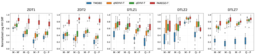
Figure 2: Box plots for 20 synthetic problems derived from ZDT1, ZDT2, DTLZ1, DTLZ2, and DTLZ7. Each algorithm runs for 20 independent trials. The logarithm of HV difference is computed at the end of each trial and is normalized between $[0,1]$.

We select five widely used multi-objective benchmark problems from ZDT [47] and DTLZ [11] test suites with $d=5$ and add Gaussian noise with a standard deviation of $1\%$ of the range of each objective. Each subplot of Figure 2 depicts the box plots over four synthetic problems with different trajectory characteristics derived from the same multi-objective benchmark. For instance, “ZDT1(M-P)” refers to the synthetic test problem derived from ZDT1 with the first objective multiplied by the monotonic curve function and the second objective by the periodic curve function. It can be observed that with a maximum budget of $150$ iterations (or the number of times the iterative learning procedure is executed), TMOBO consistently achieves the lowest HV difference among all synthetic problems, and the solutions obtained by TMOBO generally dominate a large proportion of those obtained by alternative algorithms that do not exploit trajectory information. After being enhanced by trajectory observations, the performance of two HV-based methods, $q$NEHVI-T and $q$EHVI-T, is comparable to TMOBO on ZDT2(M-M) and ZDT2(M-Q) while ParEGO-T has the worst performance. These findings indicate that the trajectory information is beneficial to the optimization of EMOHPO and that TMOBO is able to maintain its advantages when processing trajectories with even complicated characteristics. See Appendix D for more experimental results.

6.2 Experiments On Hyperparameter Tuning Benchmarks

The performance of TMOBO is further examined on five different Multi-Layer Perceptron (MLP) hyperparameter tuning tasks obtained from LCBench [46], each of which aims to optimize five hyperparameters (i.e., learning rate, momentum, weight decay, max dropout rate, and max number of units) by minimizing validation loss and training cost simultaneously on a specific training dataset. As the previous work did [14, 26, 10, 31], we utilize the surrogate version of LCBench implemented in YAHPO Gym [32] and HPOBench [12], where the performance metrics (i.e., objectives) are approximated by a high-quality surrogate, in order to avoid biased implementation errors, to run more tests, and to make sure that the experiments are reproducible in any environments (see Appendix C.2). On each dataset, we observe epoch-wise model performance for any feasible hyperparameter settings up to $50$ epochs.

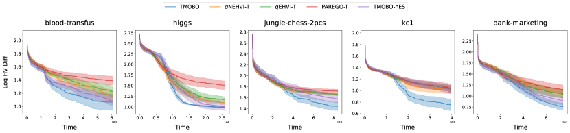
Figure 3: Average log Hypervolume difference against time for each algorithm on five different hyperparameter tuning tasks. Each algorithm runs for 20 independent trials. The shaded region indicates two standard errors of the mean.

For each task, Figure 3 plots the performance of each algorithm against time over 20 independent replications. In our analysis, we exclude the algorithm computation overhead and prioritize the cumulative model training time as the latter is the most computationally expensive part and typically dominates the total time spent on hyperparameter optimization. This ensures a clearer understanding of how optimization efforts scale with the model complexity, thereby facilitating a more insightful comparison across different models and optimization methods. Besides the enhanced MOBO methods, we also implement a variant of TMOBO, named TMOBO-nES, which does not have an early stopping mechanism and trains each sampled setting for the maximum number of epochs. We note that TMOBO and TMOBO-nES spend more time in initialization as they train the initial settings thoroughly to capture the trajectory characteristics at the initial stage. Despite the initialization, given the same wall-clock time budget, TMOBO achieves significantly lower HV difference than the other enhanced MOBO methods across all tasks. In the meantime, the average performance of TMOBO surpasses its variant TMOBO-nES, which shows the advantage of using an early stopping mechanism. While TMOBO-nES aims to learn better about trajectory characteristics through full model training, the early stopping mechanism enables TMOBO to save effort by terminating non-contributed training to explore more regions of interest.

7 Conclusions

In this study, we consider multi-objective hyperparameter optimization with iterative learning procedures. Our interest centers on how trajectory information affects the distribution of trade-offs and on how to leverage this information to perform an effective and efficient search for trade-offs. To this end, we extend the conventional MOHPO problem to EMOHPO by including the training epoch as an explicit decision variable so as to reveal the trade-offs that may occur along trajectories. These frequently overlooked trade-offs play a beneficial role in decision-making for ML model deployment with retraining schemes. As there are no algorithms specially designed to handle EMOHPO, we then propose the TMOBO algorithm to first sample the hyperparameter setting with the largest trajectory-based contribution and then determine when to early stop the training with it based on the trajectory predictions of GP models.

Through numerical experiments on synthetic simulations and hyperparameter tuning benchmarks, TMOBO has demonstrated its advantage in locating better solutions by exploiting the trajectory information compared to traditional multi-objective optimization methods. Considering that the iterative processing procedure inherent in many real-world simulations or experiments, such as drug design and material engineering, shares similar characteristics with the training of ML models, it is meaningful to explore the formulation of EMOHPO problems across a variety of practical scenarios and to extend the success of TMOBO algorithm in this study. However, optimizing the TEHVI acquisition function remains challenging. Therefore, further exploitation is needed to derive an analytical form of TEHVI or to develop more efficient approximations. Another research direction involves examining how the integration of dependent objectives or learning curves into GP modeling as well as the optimization framework can further enhance the decision-making processes.

8 Acknowledgement

We would like to thank Songhao Wang and Haowei Wang for their helpful discussions about this study. Szu Hui Ng’s work is supported in part by the Ministry of Education, Singapore (Grant: R-266-000-149-114).

 
Supplementary Material for
Trajectory-Based Multi-Objective Hyperparameter Optimization for Model Retraining
 

Appendix A Proof for Theorem 1

Recall that Theorem 1 claims that the Pareto-optimal set of $X_{Trj}^{*}\times\mathbb{T}$ is equal to the Pareto-optimal set of EMOHPO, where $X_{Trj}^{*}=\{\bm{x}\mid\bm{x}\in\mathbb{X},\exists t\in\mathbb{T},\nexists(\bm{x}^{\prime},t^{\prime})\in\mathbb{X}\times\mathbb{T},\bm{f}(\bm{x}^{\prime},t^{\prime})\prec\bm{f}(\bm{x},t)\}$. We start by establishing the following lemma.

Lemma 1.

Let $Z\subset\mathbb{R}^{d}$ and $Z^{*}$ denote its Pareto-optimal set. If $Z_{U}$ is a subset of $Z$ such that $Z^{*}\subseteq Z_{U}\subseteq Z$, the Pareto-optimal set of $Z_{U}$, denoted by $Z_{U}^{*}$, is equal to $Z^{*}$, i.e., $Z_{U}^{*}=Z^{*}$.

Proof. As per Definition 2, we have,

$$Z^{*}=\{\bm{z}\mid\bm{z}\in Z,\nexists\bm{z}^{\prime}\in Z,\bm{f}(\bm{z}^{\prime})\prec\bm{f}(\bm{z})\}$$ (8)

and

$$Z_{U}^{*}=\{\bm{z}\mid\bm{z}\in Z_{U},\nexists\bm{z}^{\prime}\in Z_{U},\bm{f}(\bm{z}^{\prime})\prec\bm{f}(\bm{z})\}.$$ (9)

(a) Let $\bm{z}\in Z^{*}\subseteq Z_{U}$. There does not exist $\bm{z}^{\prime}\in Z$ such that $\bm{f}(\bm{z}^{\prime})\prec\bm{f}(\bm{z})$. Since $Z_{U}\subseteq Z$, there does not exist $\bm{z}^{\prime}\in Z_{U}$ such that $\bm{f}(\bm{z}^{\prime})\prec\bm{f}(\bm{z})$. By (9), $\bm{z}\in Z_{U}^{*}$ and hence $Z^{*}\subseteq Z_{U}^{*}$.

(b) Assume that $Z_{U}^{*}\not\subseteq Z^{*}$. Then, there exists $\bm{z}$ satisfying

1. $\bm{z}\in Z_{U}^{*}$ $\Rightarrow$ $\nexists\bm{z}^{\prime}\in Z_{U}$ such that $\bm{f}(\bm{z}^{\prime})\prec\bm{f}(\bm{z})$;
   

2. $\bm{z}\not\in Z^{*}$ $\Rightarrow$ $\exists\bm{z}^{\prime\prime}\in Z$ such that $\bm{f}(\bm{z}^{\prime\prime})\prec\bm{f}(\bm{z})$.

Therefore, $\exists\bm{z}^{\prime\prime}\in Z\setminus Z_{U}$ such that $\bm{f}(\bm{z}^{\prime})\prec\bm{f}(\bm{z})$. Since $Z^{*}\subseteq Z_{U}$, $Z^{*}\cap(Z\setminus Z_{U})=\emptyset$ and $\bm{z}^{\prime\prime}\not\in Z^{*}$. Then, $\exists\bm{z}^{\prime\prime\prime}\in Z^{*}\subseteq Z_{U}$ such that $\bm{f}(\bm{z}^{\prime\prime\prime})\prec\bm{f}(\bm{z}^{\prime\prime})\prec\bm{f}(\bm{z})$, which contradicts to the first condition $\bm{z}\in Z_{U}^{*}$. Therefore, $Z_{U}^{*}\subseteq Z^{*}$.

Combining these two inclusions together, we conclude that $Z_{U}^{*}=Z^{*}$. ∎

As each query pair $\bm{z}=\{\bm{x},t\}$, the Pareto-optimal set $Z^{*}$ of EMOHPO defined in Definition 2 can be equivalently expressed as,

$$Z^{*}=\{(\bm{x},t)\mid(\bm{x},t)\in\mathbb{X}\times\mathbb{T},\nexists(\bm{x}^{\prime},t^{\prime})\in\mathbb{X}\times\mathbb{T},\bm{f}(\bm{x}^{\prime},t^{\prime})\prec\bm{f}(\bm{x},t)\}.$$ (10)

Then, we have,

$$Z^{*} \subseteq\{(\bm{x},t^{\prime\prime})\mid\bm{x}\in\mathbb{X},\exists t\in\mathbb{T},(\bm{x},t)\in Z^{*},t^{\prime\prime}\in\mathbb{T}\}$$ (11)

$$=\{\bm{x}\mid\bm{x}\in\mathbb{X},\exists t\in\mathbb{T},(\bm{x},t)\in Z^{*}\}\times\{t^{\prime\prime}\mid t^{\prime\prime}\in\mathbb{T}\}=X_{Trj}^{*}\times\mathbb{T}.$$

Since $Z^{*}\subseteq X_{Trj}^{*}\times\mathbb{T}\subset\mathbb{X}\times\mathbb{T}$, we complete the proof by applying Lemma 1.

Appendix B Additional Algorithm Details

Acquisition function plays a critical part in the BO framework but maximizing it presents inherent challenges. As discussed in Section 5.1, the TEHVI acquisition function extended from EHVI has no known analytical form and is multi-modal. Furthermore, approximating TEHVI by the MC method in (6) incurs significant computational overhead, making it hard to optimize efficiently. To this end, our algorithm TMOBO adopts a candidate search to determine new hyperparameter settings by strategic sampling instead of iterative optimization of the acquisition function. The candidate search first proposed by Regis and Shoemaker [34] aims to generate a set of random settings (termed as “candidates”) around a previously visited high-quality hyperparameter setting (termed as “center”). The new hyperparameter setting is then selected from these candidates by comparing their respective acquisition function values. This approach has demonstrated its effectiveness in global optimization [34] and has been extended to multi-objective cases in [43, 42]. The specific implementation details of the candidate search in TMOBO are provided below:

Center Selection. The effectiveness of a candidate search largely depends on the quality of the center chosen from previously visited hyperparameter settings. Intuitively, the trajectories of candidates near a high-quality center have a high chance of improving the current front $F$. However, it is inappropriate to directly use TEHVI to distinguish the best hyperparameter setting that has been visited, as trajectories of the visited hyperparameter settings have already contributed to constructing the front. Instead, similar to Def 4, we evaluate the contribution of a visited hyperparameter setting $\bm{x}$ by the difference between the HV of the front $F$ and it excluding the observed trajectory of $\bm{x}$. Therefore, the center is selected as,

$$\bm{x}^{c}=\operatorname*{argmax}_{\bm{x}\in X}~{}\big{[}HV\big{(}F\mid\bm{r}\big{)}-HV\big{(}F\setminus\big{\{}\bm{y}(\bm{x},t)\big{\}}_{t=0}^{t^{\prime}_{max}}\mid\bm{r}\big{)}\big{]},$$ (12)

where $\bm{r}$ denotes the reference point and $\{\bm{y}(\bm{x},t)\}_{t=1}^{t^{\prime}_{max}}$ denotes the observed trajectory when training the model with $\bm{x}$ up to $t^{\prime}_{max}$ epochs. Note that $t^{\prime}_{max}\leq t_{max}$ due to the early stopping mechanism.

Candidate Generation. After selecting the center $\bm{x}^{c}$, we generate a candidate $\bar{\bm{x}}$ by adding Gaussian perturbation with zero mean and covariance matrix $\gamma^{2}(\bm{x}^{c})I^{d}$ to the center, i.e., $\bar{\bm{x}}\sim\mathcal{N}(\bm{x}^{c},\gamma^{2}(\bm{x}^{c})I^{d})$, where $\gamma(\bm{x}^{c})$ denote the search radius specified for $\bm{x}^{c}$ with $\gamma_{max}$ being the initial value. Let $\bar{X}$ denote the set of $q$ independently generated candidates. Moreover, to dynamically balance exploration and exploitation, if the candidate search led by center $\bm{x}^{c}$ finally fails to yield a new setting to improve the front $F$, we halve its search radius so as to prioritize the points closer to it, and if the search fails for multiple times, we exclude $\bm{x}^{c}$ as a center in the subsequent iterations. Finally, we calculate the TEHVI value for each candidate in $\bar{X}$ and select the one with the highest TEHVI value to train the ML model in the current iteration.

Appendix C Experiment Setup

C.1 Algorithm Configurations

The Python implementation for TMOBO will be made openly available upon publication. Within the candidate search strategy of TMOBO, the initial search radius $\gamma_{max}$ associated with any visited hyperparameter setting is set to $0.2$ as recommended by [34]. Moreover, to ensure a sufficiently dense neighborhood around the center, the number of candidates $q$ generated around a center is set to $100d$. Then, in the early stopping mechanism, we determine the conservative stopping epoch in a way similar to computing the lower confidence bound and maintain a fixed value of $\beta$, which controls the confidence level, at $2.0$. Finally, at the end of each iteration, TMOBO takes an active data augmentation method to minimize the prediction uncertainty of the GP model by using only a subset of trajectory observations. To maintain the GP training efficiency, we limit the size of this subset to a maximum of $10$.

We use the open-source Python implementations for ParEGO, $q$EHVI, and $q$NEHVI from the BoTorch library (accessible at https://github.com/pytorch/botorch under MIT License) and adhere to the default algorithm configurations. The enhanced versions of the alternative algorithms, namely ParEGO-T, $q$EHVI-T, and $q$NEHVI-T, are implemented by collecting all the intermediate observations $\{\bm{y}(\bm{x},1),\dots,\bm{y}(\bm{x},t)\}$ to refine the current front whenever a query pair $(\bm{x},t)$ is sampled.

In each experimental trial, we initialize each algorithm with $2(d+1)$ samples drawn from a Sobol sequence. For the approximation of the acquisition function by Monte Carlo integration, we consistently employ $128$ MC samples across all iterations. HV-based acquisition functions in $q$EHVI, $q$NEHVI, and TMOBO are inherently sensitive to the choice of the reference point $\bm{r}$. However, determining an appropriate reference point generally requires prior knowledge of the problem, which is unrealistic for real-world applications. Thus, we adopt an adaptive strategy for all algorithms where each element of the reference point is continuously updated to the corresponding worst values encountered thus far. All experiments are run on a GeForce RTX 2080 Ti GPU with 11GB RAM.

C.2 Problems and Benchmarks

The classical multi-objective optimization benchmarks used to formulate the synthetic test problems in numerical experiments are provided below:

ZDT1 Benchmark [47]:

$$\min_{\bm{x}}~{}[f_{1}(\bm{x}),f_{2}(\bm{x})],$$ (13)

$$f_{1}(\bm{x})=x_{1},$$

$$f_{2}(\bm{x})=u(\bm{x})\left[1-\sqrt{x_{1}/u(\bm{x})}\right]$$

where

$$u(\bm{x})=1+\frac{9}{d-1}\sum_{i=2}^{d}x_{d},$$

and $\bm{x}=[x_{1},\dots,x_{d}]\in[0,1]^{d}$. This benchmark has a convex Pareto-optimal front with Pareto-optimal solutions being $0\leq x_{1}^{*}\leq 1$ and $x_{i}^{*}=0$ for $i=2,\dots,d$.

ZDT2 Benchmark [47]:

$$\min_{\bm{x}}~{}[f_{1}(\bm{x}),f_{2}(\bm{x})],$$ (14)

$$f_{1}(\bm{x})=x_{1},$$

$$f_{2}(\bm{x})=u(\bm{x})\left[1-(x_{1}/u(\bm{x}))^{2}\right],$$

where

$$u(\bm{x})=1+\frac{9}{d-1}\sum_{i=2}^{d}x_{d},$$

and $\bm{x}=[x_{1},\dots,x_{d}]\in[0,1]^{d}$. This benchmark has a concave Pareto-optimal front with Pareto-optimal solutions being $0\leq x_{1}^{*}\leq 1$ and $x_{i}^{*}=0$ for $i=2,\dots,d$.

DTLZ1 Benchmark [11]:

$$\min_{\bm{x}}~{}[f_{1}(\bm{x}),\dots,f_{k}(\bm{x})],$$ (15)

$$f_{1}(\bm{x})=\frac{1}{2}x_{1}x_{2}\cdots x_{k-1}(1+u(\bm{x}_{k})),$$

$$f_{2}(\bm{x})=\frac{1}{2}x_{1}x_{2}\cdots(1-x_{k-1})(1+u(\bm{x}_{k})),$$

$$~{}~{}~{}~{}~{}~{}~{}~{}~{}~{}~{}~{}\vdots$$

$$f_{k-1}(\bm{x})=\frac{1}{2}x_{1}(1-x_{2})(1+u(\bm{x}_{k})),$$

$$f_{k}(\bm{x})=\frac{1}{2}(1-x_{1})(1+u(\bm{x}_{k})),$$

where

$$u(\bm{x}_{k})=100\left[|\bm{x}_{k}|+\sum_{x_{i}\in\bm{x}_{k}}(x_{i}-0.5)^{2}-\cos(20\pi(x_{i}-0.5))\right],$$

$\bm{x}=[x_{1},\dots,x_{d}]\in[0,1]^{d}$ and $\bm{x}_{k}$ denotes the last $(d-k+1)$ variables of $\bm{x}$. The search space of this benchmark contains multiple local Pareto-optimal fronts. The global Pareto-optimal front is a linear hyperplane with Pareto-optimal solutions being $x_{i}^{*}=0.5$ for $x_{i}\in\bm{x}_{k}$.

DTLZ2 Benchmark [11]:

$$\min_{\bm{x}}~{}[f_{1}(\bm{x}),\dots,f_{k}(\bm{x})],$$ (16)

$$f_{1}(\bm{x})=\cos(\pi x_{1}/2)\cos(\pi x_{2}/2)\cdots\cos(\pi x_{k-1}/2)(1+u(\bm{x}_{k})),$$

$$f_{2}(\bm{x})=\cos(\pi x_{1}/2)\sin(\pi x_{2}/2)\cdots\cos(\pi x_{k-1}/2)(1+u(\bm{x}_{k})),$$

$$~{}~{}~{}~{}~{}~{}~{}~{}~{}~{}~{}~{}\vdots$$

$$f_{k-1}(\bm{x})=\cos(\pi x_{1}/2)\sin(\pi x_{2}/2)(1+u(\bm{x}_{k})),$$

$$f_{k}(\bm{x})=\sin(\pi x_{1}/2)(1+u(\bm{x}_{k})),$$

where

$$u(\bm{x}_{k})=\sum_{x_{i}\in\bm{x}_{k}}(x_{i}-0.5)^{2},$$

$\bm{x}=[x_{1},\dots,x_{d}]\in[0,1]^{d}$ and $\bm{x}_{k}$ denotes the last $(d-k+1)$ variables of $\bm{x}$. This benchmark has a concave Pareto-optimal front with Pareto-optimal solutions being $x_{i}^{*}=0.5$ for $x_{i}\in\bm{x}_{k}$.

DTLZ7 Benchmark [11]:

$$\min_{\bm{x}}~{}[f_{1}(\bm{x}),\dots,f_{k}(\bm{x})],$$ (17)

$$f_{1}(\bm{x})=x_{1},$$

$$~{}~{}~{}~{}~{}~{}~{}~{}~{}~{}~{}~{}\vdots$$

$$f_{k-1}(\bm{x})=x_{k-1},$$

$$f_{k}(\bm{x})=h(f_{1},f_{2},\dots,f_{k-1},u)(1+u(\bm{x}_{k})),$$

where

$$u(\bm{x}_{k})=1+\frac{9}{|\bm{x}_{k}|}\sum_{x_{i}\in\bm{x}_{k}}x_{i},$$

$$h(f_{1},f_{2},\dots,f_{k-1},u)=k-\sum_{i=1}^{k-1}\left[\frac{f_{i}}{1+u}(1+\sin(3\pi f_{i}))\right],$$

$\bm{x}=[x_{1},\dots,x_{d}]\in[0,1]^{d}$ and $\bm{x}_{k}$ denotes the last $(d-k+1)$ variables of $\bm{x}$. The Pareto-optimal front of this benchmark is composed of $2^{k-1}$ disconnected regions with Pareto-optimal solutions being $x_{i}^{*}=0$ for $x_{i}\in\bm{x}_{k}$.

Given the $i$-th objective function $f_{i}(\bm{x})$ of any benchmark above, we construct its epoch-dependent counterpart as $f_{i}(\bm{x},t)=f_{i}(\bm{x})\cdot g_{i}(t)$ to simulate the training procedure by the curve function $g_{i}(t)$. In our experiments, we utilize different curve functions to diversify the learning curve characteristics, and these functions are,

• Monotonically Increasing Curve: $g^{M}(t\mid t_{max})=0.5+1/\left(1+e^{(-0.2(t-t_{max}/2))}\right)$,
  

• Monotonically Decreasing Curve: $g^{M^{\prime}}(t\mid t_{max})=0.3+1/\left(1+e^{(0.1(t-t_{max}/3))}\right)$,
  

• Quadratic Curve: $g^{Q}(t\mid t_{max})=0.5+2\left(t/t_{max}-2/3\right)^{2}$,
  

• Periodic Curve: $g^{P}(t\mid t_{max})=1+0.5\sin(4\pi t/t_{max})$,

where $t\in\mathbb{T}=[1,2,\dots,t_{max}]$ and $t_{max}=50$.

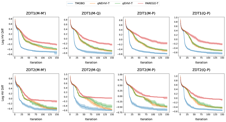
Figure 4: Average log Hypervolume difference against iterations for each algorithm on synthetic problems generated from ZDT1 and ZDT2. Each algorithm runs for 20 independent trials. The shaded region indicates two standard errors of the mean.

LCBench [46]: This benchmark is designed to give insights on multi-fidelity optimization with learning curves for Auto Deep Learning. LCBench was originally developed upon tabular data. Benefitting from the surrogate implementation by HPOBench (under Apache License 2.0) [12] and YAHPO Gym (under Apache License 2.0) [32], we are allowed to observe the intermediate model performance for any feasible hyperparameter setting after each epoch. The maximum number of epochs for training MLP is set to $50$. We choose to minimize validation loss and training time, which are commonly considered in many MOHPO studies. For a demonstration, we focus on tuning the five hyperparameters (i.e., $d=5$) of MLP including learning rate in $[1\times 10^{-4},1\times 10^{-1}]$, momentum in $[0.10,0.99]$, weight decay in $[1\times 10^{-5},1\times 10^{-1}]$, maximum dropout rate in $[0.0,1.0]$, and maximum number of neurons in $[64,1024]$. LCBench utilizes diverse datasets from AutoML Benchmark [15] hosted on OpenML [41]. For experimentation, we select “blood-transfus”, “higgs”, “jungle-chess-2pcs”, “kc1”, and “banck-marketing”, each of which has at least two attributes and between 500 and 1,000,000 data points.

Appendix D Additional Numerical Results

This section presents additional numerical results comparing TMOBO with three enhanced multi-objective optimization methods. It is noteworthy that all the algorithms follow a similar routine in each iteration: upon sampling a new hyperparameter setting, the training procedure for the corresponding ML model starts to proceed by epochs. The difference is that TMOBO dynamically determines the stopping epoch during training while the others determine it before training begins. By tracking the number of times of model training, Figure 4 and 5 depicts the performance of each algorithm against the number of iterations on 20 synthetic problems analyzed in Section 6.1. The four subplots in each row represent synthetic problems derived from the same multi-objective benchmark but with different trajectory characteristics.

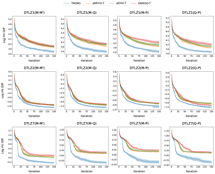
Figure 5: Average log Hypervolume difference against iterations for each algorithm on synthetic problems generated from DTLZ1, DTLZ2, and DTLZ7. Each algorithm runs for 20 independent trials. The shaded region indicates two standard errors of the mean.

Firstly, on variants of two relatively simple ZDT benchmarks (in Figure 4), TMOBO quickly converges to a small HV difference value after executing a small number of iterations, and it maintains the lowest average HV difference until the end. Among the alternatives, the HV-based methods, $q$NEHVI-T and $q$EHVI-T, perform better and can find solutions that are comparable to TMOBO on the first two instances of ZDT2; however, as the trajectory characteristics become more complex, both algorithms are dominated by TMOBO.

On variants of DTLZ benchmarks (in Figure 5), the difference between TMOBO and alternatives becomes larger, especially on the rows of DTLZ1 and DTLZ7, while the alternatives show similar performances to each other. On the synthetic problems derived from DTLZ1, all the algorithms struggle to converge adequately within 150 iterations, primarily because the DTLZ1 benchmark has multiple local optima. However, through the trials, the HV difference values reached by TMOBO are significantly better than the alternatives. Additionally, the DTLZ7 benchmark has a disconnected Pareto-optimal front and it challenges the capability of optimizers to maintain a diverse set of solutions. Notably, TMOBO emerges as the best choice for handling this type of challenge, as the alternatives tend to stagnate at relatively high HV difference values at an early stage.

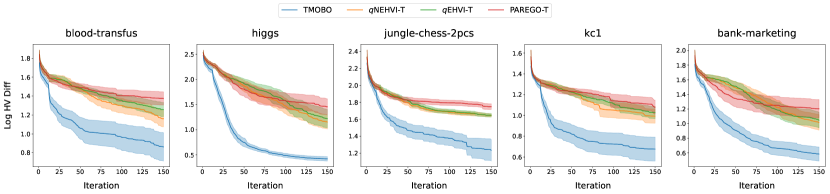
Figure 6: Average log Hypervolume difference against iterations for each algorithm on five different hyperparameter tuning tasks. Each algorithm runs for 20 independent trials. The shaded region indicates two standard errors of the mean.

Finally, on the five LCBench hyperparameter tuning tasks analyzed in Section 6.2, we also show the performance of algorithms against iterations in Figure 6. Similar to the comparison results based on time, when given the same number of iterations, TMOBO consistently achieves the smallest HV difference values throughout. In other words, the Pareto-optimal fronts found by TMOBO are not only better converged but also more diversified compared to those found by the alternatives.

Appendix E Replication Strategy

Replicated observations at a query $(\bm{x},t)$ might be needed to achieve adequate accuracy, especially in the presence of significant noises. While this particular scenario is not the focus of our current study, we outline a straightforward method to extend the proposed TMOBO to accommodate the requirement for replicated observations when the computational budget is sufficient. It is essential to recognize that with each noisy observation obtained at $(\bm{x},t)$, the training process must start from scratch and will also output noisy observations from $(\bm{x},1)$ up to $(\bm{x},t-1)$. As a consequence, careful maintenance of multiple training procedures for replications is needed to ensure algorithmic efficiency. The pseudo-code for TMOBO-$P$, a modified version of TMOBO, is presented in Algorithm 2.

Algorithm 2 Framework of TMOBO-$P$

Input: Initial sets of inputs $Z$ and observations $Y$, number of replications $P$, and initial Pareto-optimal front $F$ identified from $Y$.

1:while the computational budget has not been exceeded do

2:     Fit $k$ GP models with $\bm{\mu}$ and $\bm{\Sigma}$ based on sets $Z$ and $Y$.

3:     Sample a new $\bm{x}^{\prime}$ by maximizing the TEHVI acquisition function.

4:     Initialize $Z^{\prime}\leftarrow\emptyset$ and $Y^{\prime}\leftarrow\emptyset$.

5:     for $t^{\prime}=1$ to $t_{\max}$ do

6:         for $p=1$ to $P$ do

7:              Continue model training for the $t^{\prime}$-th epoch to obtain observation $\bm{y}_{p}(\bm{x}^{\prime},t^{\prime})$ on the $p$-th processor.

8:         end for

9:         Let $Z^{\prime}\leftarrow Z^{\prime}\cup\{(\bm{x}^{\prime},t^{\prime})\}$ and $Y^{\prime}\leftarrow Y^{\prime}\cup\{\sum_{p=1}^{P}\bm{y}_{p}(\bm{x}^{\prime},t^{\prime})/P\}$ and update front $F$.

10:         Fit $k$ GP models with $\bm{\mu}$ and $\bm{\Sigma}$ based on sets $Z\cup Z^{\prime}$ and $Y\cup Y^{\prime}$.

11:         if EarlyStopping$(\bm{x}^{\prime},t^{\prime},\bm{\mu},\bm{\Sigma},F)$ is triggered then

12:              Break;

13:         end if

14:     end for

15:     Augment $Z^{\prime}$ and $Y^{\prime}$ into $Z$ and $Y$ respectively.

16:end while

With an additional input $P$ denoting the number of replications, TMOBO-$P$ intends to include $P$ replicated observations at any visited query pair to mitigate the influence of noises. In each iteration, different from TMOBO, TMOBO-$P$ concurrently tracks $P$ independent training procedures for the ML model with the same sampled hyperparameter setting $\bm{x}^{\prime}$ and ensures their progress remains consistent at the same epoch. Therefore, upon visiting a query pair $(\bm{x},t^{\prime})$, we can obtain $P$ replicated observations of it. Intuitively, the collection of sample means $\{\sum_{p=1}^{P}\bm{y}_{p}(\bm{x}^{\prime},1)/P,\dots,\sum_{p=1}^{P}\bm{y}_{p}(\bm{x}^{\prime},t_{max})/P\}$ form a compressed trajectory of $\bm{x}^{\prime}$, i.e., average of $P$ observed trajectory of $\bm{x}^{\prime}$. Then, the early stopping mechanism is applied to the compressed trajectory to determine when to stop all $P$ training procedures at the same time. Since the replicated training procedures are independent, TMOBO-$P$ can leverage parallel computing by assigning each training procedure to a specific processor.

Figure 7 shows the performance of TMOBO-$P$ with $P=1$, $4$, $16$, and $64$ on the synthetic problems derived from ZDT1. TMOBO proposed in the main paper can be considered a special case of TMOBO-$P$ with $P=1$. This time, we add Gaussian noise to each objective with a standard deviation of $10\%$ of the objective range in order to emphasize the influence of noises. It can be observed that the performance of TMOBO-$P$ improves significantly in terms of the HV difference as more replications are allowed. This improvement is evident not only in rapid convergence during the initial stages but also in obtaining high-quality results at the end when comparing TMOBO with $P\geq 16$ to TMOBO with $P<16$. In the meantime, benefiting from a large number of replications, TMOBO-$64$ has stable performance and its standard error is relatively small.

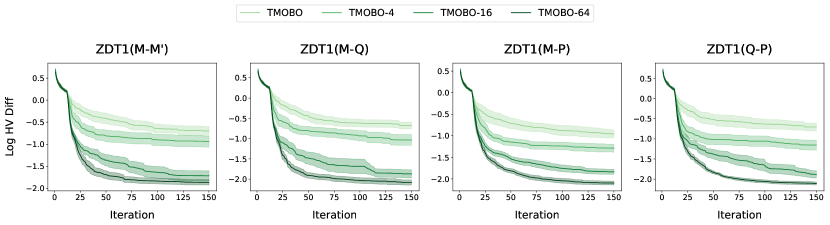
Figure 7: Average log Hypervolume difference against iterations for each algorithm on synthetic problems generated from ZDT1 with $10\%$ noise level. Each algorithm runs for 20 independent trials. The shaded region indicates two standard errors of the mean.

References

- Belakaria et al. [2019] Syrine Belakaria, Aryan Deshwal, and Janardhan Rao Doppa. Max-value entropy search for multi-objective bayesian optimization. In Advances in Neural Information Processing Systems, volume 32, 2019.
- Belakaria et al. [2020] Syrine Belakaria, Aryan Deshwal, and Janardhan Rao Doppa. Multi-fidelity multi-objective bayesian optimization: An output space entropy search approach. In Proceedings of the AAAI Conference on artificial intelligence, volume 34, pages 10035–10043, 2020.
- Belakaria et al. [2023] Syrine Belakaria, Janardhan Rao Doppa, Nicolo Fusi, and Rishit Sheth. Bayesian optimization over iterative learners with structured responses: A budget-aware planning approach. In Proceedings of The 26th International Conference on Artificial Intelligence and Statistics, pages 9076–9093. PMLR, 2023.
- Bergstra et al. [2011] James Bergstra, Rémi Bardenet, Yoshua Bengio, and Balázs Kégl. Algorithms for hyper-parameter optimization. In Advances in Neural Information Processing Systems, volume 24, 2011.
- Casimiro et al. [2020] Maria Casimiro, Diego Didona, Paolo Romano, Luis Rodrigues, Willy Zwaenepoel, and David Garlan. Lynceus: Cost-efficient tuning and provisioning of data analytic jobs. In 2020 IEEE 40th International Conference on Distributed Computing Systems (ICDCS), pages 56–66. IEEE, 2020.
- Casimiro et al. [2024] Maria Casimiro, Diogo Soares, David Garlan, Luís Rodrigues, and Paolo Romano. Self-adapting machine learning-based systems via a probabilistic model checking framework. ACM Transactions on Autonomous and Adaptive Systems, 2024.
- Dai et al. [2019] Zhongxiang Dai, Haibin Yu, Bryan Kian Hsiang Low, and Patrick Jaillet. Bayesian optimization meets bayesian optimal stopping. In Proceedings of the 36th International Conference on Machine Learning, volume 97, pages 1496–1506. PMLR, 2019.
- Daulton et al. [2020] Samuel Daulton, Maximilian Balandat, and Eytan Bakshy. Differentiable expected hypervolume improvement for parallel multi-objective bayesian optimization. In Advances in Neural Information Processing Systems, volume 33, pages 9851–9864, 2020.
- Daulton et al. [2021] Samuel Daulton, Maximilian Balandat, and Eytan Bakshy. Parallel bayesian optimization of multiple noisy objectives with expected hypervolume improvement. In Advances in Neural Information Processing Systems, volume 34, pages 2187–2200, 2021.
- Daxberger et al. [2019] Erik Daxberger, Anastasia Makarova, Matteo Turchetta, and Andreas Krause. Mixed-variable bayesian optimization. arXiv preprint arXiv:1907.01329, 2019.
- Deb et al. [2002] Kalyanmoy Deb, Lothar Thiele, Marco Laumanns, and Eckart Zitzler. Scalable multi-objective optimization test problems. In Proceedings of the 2002 Congress on Evolutionary Computation. CEC’02 (Cat. No. 02TH8600), volume 1, pages 825–830. IEEE, 2002.
- Eggensperger et al. [2021] Katharina Eggensperger, Philipp Müller, Neeratyoy Mallik, Matthias Feurer, René Sass, Aaron Klein, Noor Awad, Marius Lindauer, and Frank Hutter. Hpobench: A collection of reproducible multi-fidelity benchmark problems for hpo. In Thirty-fifth Conference on Neural Information Processing Systems Datasets and Benchmarks Track (Round 2), 2021.
- Emmerich et al. [2006] Michael TM Emmerich, Kyriakos C Giannakoglou, and Boris Naujoks. Single-and multiobjective evolutionary optimization assisted by gaussian random field metamodels. IEEE Transactions on Evolutionary Computation, 10(4):421–439, 2006.
- Falkner et al. [2018] Stefan Falkner, Aaron Klein, and Frank Hutter. Bohb: Robust and efficient hyperparameter optimization at scale. In Proceedings of the 35th International Conference on Machine Learning, volume 80, pages 1437–1446. PMLR, 2018.
- Gijsbers et al. [2019] Pieter Gijsbers, Erin LeDell, Janek Thomas, Sébastien Poirier, Bernd Bischl, and Joaquin Vanschoren. An open source automl benchmark. arXiv preprint arXiv:1907.00909, 2019.
- Hernández-Lobato et al. [2016] Daniel Hernández-Lobato, Jose Hernandez-Lobato, Amar Shah, and Ryan Adams. Predictive entropy search for multi-objective bayesian optimization. In Proceedings of The 33rd International Conference on Machine Learning, volume 48, pages 1492–1501. PMLR, 2016.
- Hupkens et al. [2015] Iris Hupkens, André Deutz, Kaifeng Yang, and Michael Emmerich. Faster exact algorithms for computing expected hypervolume improvement. In Proceedings of the International Conference on Evolutionary Multi-Criterion Optimization, pages 65–79. Springer, 2015.
- Jones et al. [1998] Donald R Jones, Matthias Schonlau, and William J Welch. Efficient global optimization of expensive black-box functions. Journal of Global optimization, 13:455–492, 1998.
- Kandasamy et al. [2016] Kirthevasan Kandasamy, Gautam Dasarathy, Junier B Oliva, Jeff Schneider, and Barnabás Póczos. Gaussian process bandit optimisation with multi-fidelity evaluations. In Advances in Neural Information Processing Systems, volume 29, 2016.
- Kandasamy et al. [2017] Kirthevasan Kandasamy, Gautam Dasarathy, Jeff Schneider, and Barnabás Póczos. Multi-fidelity bayesian optimisation with continuous approximations. In Proceedings of the 34th International Conference on Machine Learning, volume 70, pages 1799–1808. PMLR, 2017.
- Karl et al. [2022] Florian Karl, Tobias Pielok, Julia Moosbauer, Florian Pfisterer, Stefan Coors, Martin Binder, Lennart Schneider, Janek Thomas, Jakob Richter, Michel Lang, et al. Multi-objective hyperparameter optimization–an overview. arXiv preprint arXiv:2206.07438, 2022.
- Klein et al. [2017] Aaron Klein, Stefan Falkner, Simon Bartels, Philipp Hennig, and Frank Hutter. Fast bayesian optimization of machine learning hyperparameters on large datasets. In Proceedings of the 20th International Conference on Artificial Intelligence and Statistics, volume 54, pages 528–536. PMLR, 2017.
- Knowles [2006] Joshua Knowles. Parego: A hybrid algorithm with on-line landscape approximation for expensive multiobjective optimization problems. IEEE Transactions on Evolutionary Computation, 10(1):50–66, 2006.
- Li et al. [2018] Lisha Li, Kevin Jamieson, Giulia DeSalvo, Afshin Rostamizadeh, and Ameet Talwalkar. Hyperband: A novel bandit-based approach to hyperparameter optimization. Journal of Machine Learning Research, 18(185):1–52, 2018.
- Mahadevan and Mathioudakis [2024] Ananth Mahadevan and Michael Mathioudakis. Cost-aware retraining for machine learning. Knowledge-Based Systems, 293:111610, 2024.
- Martinez-Cantin [2018] Ruben Martinez-Cantin. Funneled bayesian optimization for design, tuning and control of autonomous systems. IEEE Transactions on Cybernetics, 49(4):1489–1500, 2018.
- Mendes et al. [2020] Pedro Mendes, Maria Casimiro, Paolo Romano, and David Garlan. Trimtuner: Efficient optimization of machine learning jobs in the cloud via sub-sampling. In 28th International Symposium on Modeling, Analysis, and Simulation of Computer and Telecommunication Systems (MASCOTS), pages 1–8. IEEE, 2020.
- Morales-Hernández et al. [2023] Alejandro Morales-Hernández, Inneke Van Nieuwenhuyse, and Sebastian Rojas Gonzalez. A survey on multi-objective hyperparameter optimization algorithms for machine learning. Artificial Intelligence Review, 56(8):8043–8093, 2023.
- Nguyen et al. [2020] Vu Nguyen, Sebastian Schulze, and Michael Osborne. Bayesian optimization for iterative learning. In Advances in Neural Information Processing Systems, volume 33, pages 9361–9371, 2020.
- Paria et al. [2020] Biswajit Paria, Kirthevasan Kandasamy, and Barnabás Póczos. A flexible framework for multi-objective bayesian optimization using random scalarizations. In Proceedings of The 35th Uncertainty in Artificial Intelligence Conference, volume 115, pages 766–776. PMLR, 2020.
- Perrone et al. [2018] Valerio Perrone, Rodolphe Jenatton, Matthias W Seeger, and Cédric Archambeau. Scalable hyperparameter transfer learning. In Advances in Neural Information Processing Systems, volume 31, 2018.
- Pfisterer et al. [2022] Florian Pfisterer, Lennart Schneider, Julia Moosbauer, Martin Binder, and Bernd Bischl. Yahpo gym-an efficient multi-objective multi-fidelity benchmark for hyperparameter optimization. In Proceedings of the First International Conference on Automated Machine Learning, volume 188, pages 1–39. PMLR, 2022.
- Rasmussen and Williams [2005] Carl Edward Rasmussen and Christopher K. I. Williams. Gaussian processes for machine learning. The MIT Press, 11 2005.
- Regis and Shoemaker [2007] Rommel G Regis and Christine A Shoemaker. A stochastic radial basis function method for the global optimization of expensive functions. INFORMS Journal on Computing, 19(4):497–509, 2007.
- Sen et al. [2018] Rajat Sen, Kirthevasan Kandasamy, and Sanjay Shakkottai. Multi-fidelity black-box optimization with hierarchical partitions. In Proceedings of the 35th International Conference on Machine Learning, volume 80, pages 4538–4547. PMLR, 2018.
- Srinivas et al. [2009] Niranjan Srinivas, Andreas Krause, Sham M Kakade, and Matthias Seeger. Gaussian process optimization in the bandit setting: No regret and experimental design. In Proceedings of the 27th International Conference on International Conference on Machine Learning, page 1015–1022, 2009.
- Suzuki et al. [2020] Shinya Suzuki, Shion Takeno, Tomoyuki Tamura, Kazuki Shitara, and Masayuki Karasuyama. Multi-objective bayesian optimization using pareto-frontier entropy. In Proceedings of the 37th International Conference on Machine Learning, volume 119, pages 9279–9288. PMLR, 2020.
- Swersky et al. [2014] Kevin Swersky, Jasper Snoek, and Ryan Prescott Adams. Freeze-thaw bayesian optimization. arXiv preprint arXiv:1406.3896, 2014.
- Takeno et al. [2020] Shion Takeno, Hitoshi Fukuoka, Yuhki Tsukada, Toshiyuki Koyama, Motoki Shiga, Ichiro Takeuchi, and Masayuki Karasuyama. Multi-fidelity bayesian optimization with max-value entropy search and its parallelization. In Proceedings of the 37th International Conference on Machine Learning, volume 119, pages 9334–9345. PMLR, 2020.
- Thompson [1933] William R Thompson. On the likelihood that one unknown probability exceeds another in view of the evidence of two samples. Biometrika, 25(3-4):285–294, 1933.
- Vanschoren et al. [2014] Joaquin Vanschoren, Jan N Van Rijn, Bernd Bischl, and Luis Torgo. Openml: networked science in machine learning. ACM SIGKDD Explorations Newsletter, 15(2):49–60, 2014.
- Wang and Shoemaker [2023] Wenyu Wang and Christine A Shoemaker. Reference vector assisted candidate search with aggregated surrogate for computationally expensive many objective optimization problems. INFORMS Journal on Computing, 35(2):318–334, 2023.
- Wang et al. [2023] Wenyu Wang, Taimoor Akhtar, and Christine A Shoemaker. Efficient multi-objective optimization through parallel surrogate-assisted local search with tabu mechanism and asynchronous option. Engineering Optimization, pages 1–17, 2023.
- Xiong et al. [2021] Yuanhao Xiong, Xuanqing Liu, Li-Cheng Lan, Yang You, Si Si, and Cho-Jui Hsieh. Rethinking the role of hyperparameter tuning in optimizer benchmarking, 2021. URL https://openreview.net/forum?id=s6M0gjo0rL0.
- Yang et al. [2022] Kaifeng Yang, Michael Affenzeller, and Guozhi Dong. A parallel technique for multi-objective bayesian global optimization: Using a batch selection of probability of improvement. Swarm and Evolutionary Computation, 75:101183, 2022.
- Zimmer et al. [2021] Lucas Zimmer, Marius Lindauer, and Frank Hutter. Auto-pytorch: Multi-fidelity metalearning for efficient and robust autodl. IEEE Transactions on Pattern Analysis and Machine Intelligence, 43(9):3079–3090, 2021.
- Zitzler et al. [2000] Eckart Zitzler, Kalyanmoy Deb, and Lothar Thiele. Comparison of multiobjective evolutionary algorithms: Empirical results. Evolutionary computation, 8(2):173–195, 2000.
- Zitzler et al. [2007] Eckart Zitzler, Dimo Brockhoff, and Lothar Thiele. The hypervolume indicator revisited: On the design of pareto-compliant indicators via weighted integration. In Proceedings of the 4th International Conference on Evolutionary Multi-Criterion Optimization, pages 862–876. Springer, 2007.