Towards Understanding How Transformer Perform Multi-step Reasoning with Matching Operation

Abstract

Large language models have consistently struggled with complex reasoning tasks, such as mathematical problem-solving. Investigating the internal reasoning mechanisms of these models can help us design better model architectures and training strategies, ultimately enhancing their reasoning capabilities. In this study, we examine the matching mechanism employed by Transformer for multi-step reasoning on a constructed dataset. We investigate factors that influence the model’s matching mechanism and discover that small initialization and post-LayerNorm can facilitate the formation of the matching mechanism, thereby enhancing the model’s reasoning ability. Moreover, we propose a method to improve the model’s reasoning capability by adding orthogonal noise. Finally, we investigate the parallel reasoning mechanism of Transformers and propose a conjecture on the upper bound of the model’s reasoning ability based on this phenomenon. These insights contribute to a deeper understanding of the reasoning processes in large language models and guide designing more effective reasoning architectures and training strategies.

1 Introduction

In recent years, LLMs have emerged and demonstrated remarkable capabilities across various tasks [1, 2, 3, 4, 5, 6]. These models have shown impressive in-context learning abilities [7, 8, 9] and have been applied to logical reasoning problems, such as matching top human contestants at the International Mathematical Olympiad (IMO) level [10] and solving math problems [11].

However, even the most advanced models still struggle with complex reasoning tasks (Fig. 1), which indicates the ability of LLMs to handle multi-step logical reasoning remains constrained. To truly enhance the reasoning capabilities of LLMs, it is crucial to investigate their intrinsic reasoning mechanisms. In this work, we focus on how LLMs process multi-step reasoning within their architecture, which can help develop more effective strategies for improving their multi-step reasoning abilities.

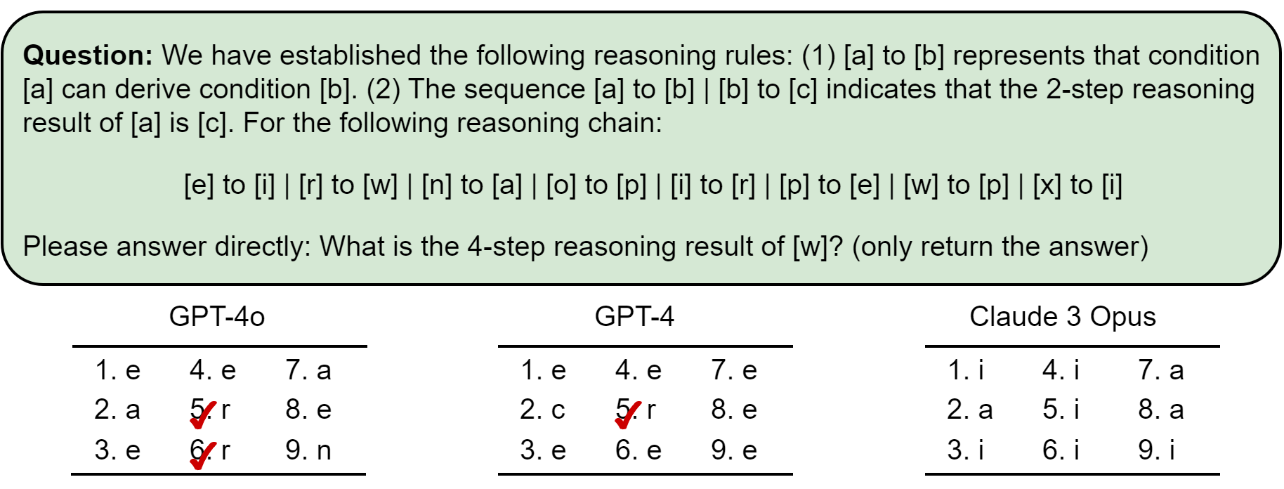
Figure 1: Failure case of multi-step reasoning in LLM. The correct answer is [r] (Since [w] $\to$ [p] $\to$ [e] $\to$ [i] $\to$ [r]). We tested each model 9 times.

Multi-step reasoning refers to the process of directly outputting the desired result by integrating the logical reasoning information flow presented in the given context. For example, if the context contains a structure like "[A]$\to$[B]...[B]$\to$[C]...[A]", where "..." represents other textual content unrelated to logical reasoning, we expect the model to directly output "[C]".

When a sentence contains only one logical reasoning step, it is often handled by the so-called induction head in Transformer[7, 12]. However, multi-step reasoning is not merely a linear accumulation of multiple induction heads but involves more complex mechanisms. Our work aims to uncover these mechanisms and provide insights into how Transformer process and integrate logical information across multiple layers to perform multi-step reasoning.

State-of-the-art models such as GPT-4 usually employ the horizontal thinking strategy, such as Chain-of-Thought (CoT) prompting[13, 14], which calls the model multiple times to generate explicit intermediate reasoning steps. This approach enhances the model’s reasoning capacity by prolonging the thought process horizontally. With the CoT prompt, all of the models can output the correct answer in the example task shown in Fig. 1. Complementary to the horizontal approach, our investigation focuses on the vertical thinking ability of Transformer models, i.e., the inherent capacity to perform multi-step reasoning within the model architecture itself. We aim to uncover how the model’s reasoning ability scales with its depth, without relying on external prompts or multiple calls. The insights from CoT prompting and our multi-step reasoning analysis offer complementary perspectives on enhancing the reasoning performance of LLMs.

To delve into the reasoning mechanisms of Transformer models, we design three types of multi-step reasoning datasets and analyze the model’s internal information flow. Our research reveals that Transformer models mainly achieve multi-step reasoning through matching operations. We propose the concept of a matching matrix to measure the model’s matching ability in each layer and find that even for untrained random embedding vectors, the model can maintain good matching ability, suggesting that Transformer models may have learned the essence of reasoning tasks.

Furthermore, we explore methods to enhance the model’s matching ability, including initialization, LayerNorm position, and adding orthogonal noise. We discover that small initialization and post-LayerNorm significantly facilitate Transformer in learning reasoning tasks. These findings provide valuable insights for designing more effective reasoning architectures and training strategies.

Lastly, we find that Transformers can perform multiple reasoning steps simultaneously within each layer when the reasoning steps exceed or equal the number of model layers, exhibiting parallel reasoning ability. This discovery inspires us to propose a conjecture on the upper bound of the reasoning ability of Transformers, suggesting that their reasoning capability may grow exponentially with the increase of model depth.

The main contributions of this work are as follows:

• We uncover the matching mechanism employed by Transformer models for multi-step reasoning and propose the concept of a matching matrix to measure the model’s matching ability.

• We discover that small initialization, post-LayerNorm, and adding orthogonal noise to certain modules of the Transformer can significantly enhance the model’s matching ability.

• We find that Transformer models can exhibit parallel reasoning capabilities. We provide an understanding of this phenomenon from the perspective of subspace division and propose a conjecture that the reasoning ability of Transformers may grow exponentially with the model depth.

Our research deepens the understanding of the reasoning mechanisms in Transformer models and provides new perspectives for further enhancing their reasoning capabilities. The insights gained from this study can contribute to the design of more efficient reasoning models and the exploration of reasoning mechanisms in general artificial intelligence systems.

2 Formulation

Dataset. To understand the mechanism of multi-step reasoning in Transformers, we design three types of multi-step reasoning tasks. As shown in Fig. 2, different reasoning chains are serialized into a sequence. Every two tokens in the sentence represent a reasoning relation. We use different labeling methods to generate the following three types of datasets:

• Type 1: The last token is the starting point, and the label is the reasoning result with a fixed-step reasoning starting from the starting point.

• Type 2: The last token is the starting point, and the label is the endpoint of the reasoning chain where the starting point is located.

• Type 3: The last two tokens are the starting point and the specified reasoning steps, respectively. The label is the reasoning result with a specified-step reasoning starting from the starting point.

We design three chain structures: single chain, double chain, and forest chain. The chain structure is unique in each task. We use the cross-entropy loss function to supervise the learning of the last token in the output sequence, rather than performing the next token prediction for all tokens.

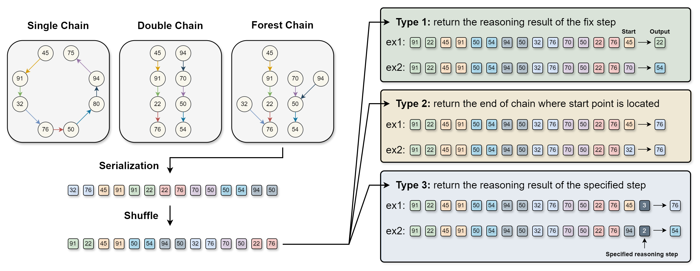
Figure 2: Illustration of the reasoning chain structures and dataset types in this study. We consider three types of reasoning chain structures: single chain, double chain, and forest chain. These structures are serialized and labeled according to different strategies, resulting in three dataset types.

Train and Test Data. We designed a method to partition the data so that every 1-step reasoning pair in the training set is different from those in the test set. Specifically, for the serialized reasoning chain [x${}_{\texttt{1}}$][x${}_{\texttt{2}}$]$\cdots$[x${}_{\texttt{n}}$] of the training set, all tokens satisfy the following condition:

$$\texttt{x}_{\texttt{2i}}-\texttt{x}_{\texttt{2i-1}}\ \ (\text{mod }5)\in[0,1,4].$$ (1)

For the reasoning chains in the test set, all tokens satisfy:

$$\texttt{x}_{\texttt{2i}}-\texttt{x}_{\texttt{2i-1}}\ \ (\text{mod }5)\in[2,3].$$ (2)

The value of each token ranges from 20 to 100, i.e., $\texttt{x}_{\texttt{i}}\in[20,100]$. Under this setting, we examine the Transformer’s ability to perform zero-shot in-context learning[7, 12], as each reasoning pair is not seen during in-weight learning.

Model Architecture. We employ a decoder-only Transformer. Given an input sequence $X^{\mathrm{in}}\in\mathbb{R}^{n\times d}$, where $n$ is the sequence length and $d$ is the dictionary size, the model first applies an embedding layer (target embedding and position embedding) to obtain the input representation $X^{(1)}=X^{\mathrm{tgt}}+X^{\mathrm{pos}}\in\mathbb{R}^{n\times d_{m}}$. The single-head attention in each layer is computed as follows:

$$\mathrm{Attn}^{(l)}=\mathrm{softmax}\left(\frac{\mathrm{mask}(X^{(l)}W^{Q(l),\mathsf{T}}W^{K(l)}X^{(l),\mathsf{T}})}{\sqrt{d_{k}}}\right),\quad X^{\mathrm{qkv}(l)}=\mathrm{Attn}^{(l)}X^{(l)}W^{V(l),\mathsf{T}},$$

where $W^{V(l),\mathsf{T}}$ represents the transpose of $W^{V(l)}$. The output of the $l$-th layer is obtained as:

$$X^{\mathrm{ao}(l)}=\text{LayerNorm}(X^{(l)}+X^{\mathrm{qkv}(l)}W^{O(l),\mathsf{T}}),\quad X^{(l+1)}=\text{LayerNorm}(\text{FNN}^{(l)}(X^{\mathrm{ao}(l)})+X^{\mathrm{ao}(l)}).$$

After that, a projection layer is applied to map the output to the target space $Y\in\mathbb{R}^{n\times d}$. The final output is obtained by taking the argmax of the softmax function applied to $Y$. A detailed description of the model architecture and notation can be found in Appendix A.

Information Flow. The information flow is constructed as follows: the $j$-th point in layer $l$ and the $i$-th point in layer $l+1$ are connected by a solid line, with the line thickness positively correlated with the value of $\mathrm{Attn}^{(l)}_{i,j}$. The intuitive and clear representation of the information flow facilitates our study of complex mechanisms such as multi-step reasoning.

3 Mechanism of Multi-Step Reasoning in Transformers

In this section, we delve into the intrinsic mechanism of multi-step reasoning by examining how a 3-layer Transformer handles 2-step Type 1 tasks. The training details can be found in Appendix D. Fig. 3 provides a visual representation of the trained model’s internal reasoning process when presented with a double-chain structured reasoning sequence.

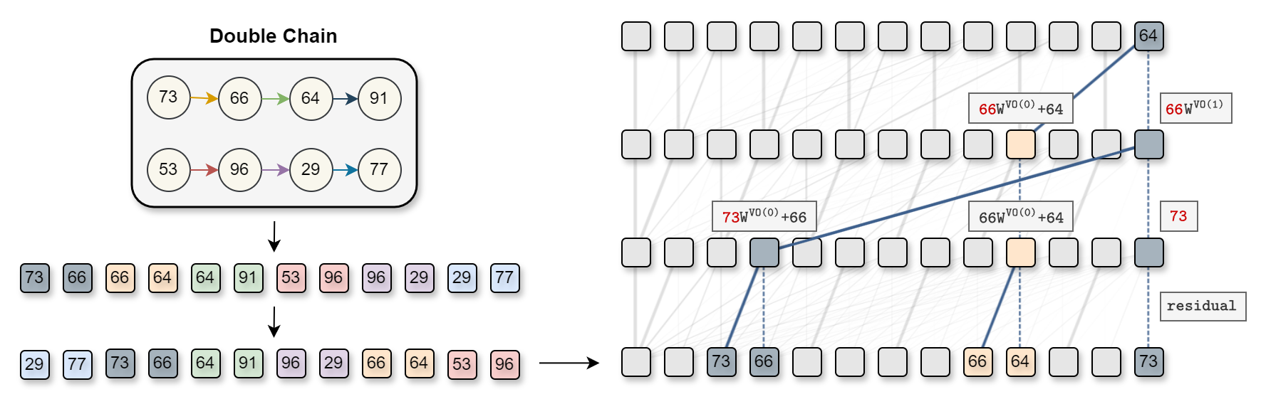
Figure 3: Information flow of a 3-layer Transformer network performing 2-step reasoning. Solid lines represent information transmission through attention, with blue solid lines indicating the attention information flow that influences the result in this example. Blue dashed lines denote the residual information flow that affects the result in this example.

Layer 0-1: Information Fusion. The primary function of the first layer is the information infusion of odd-even pairs, which is a consequence of the training set’s data structure, as odd-positioned tokens in the training sequences can infer their subsequent even-positioned tokens. This layer’s implementation mainly relies on positional embeddings. More evidence is discussed in Appendix D.

Layer 1-2: Information Matching. After information fusion, the even positions in the first layer possess information from two tokens, which are not simply added together but stored in the form of "$\texttt{[x}_{\texttt{2i-1}}\texttt{]}W^{VO(0)}+\texttt{[x}_{\texttt{2i}}\texttt{]}$", where $W^{VO(0)}=W^{V(0),\mathsf{T}}W^{O(0),\mathsf{T}}$. Consequently, a matching operation occurs in layer 1. Specifically, denoting the start point as [A], its query will have the largest inner product with the key of "$\texttt{[A]}W^{VO(0)}+\texttt{[B]}$", thereby transmitting the information of [B] to the last position. Our research reveals that this matching operation does not require the participation of "[B]" and the positional encoding of the sequence. Instead, it is achieved solely through the query of "[A]", i.e., $\text{F}^{(0)}(X^{\text{tgt}}_{\texttt{A}})W^{Q(1),\mathsf{T}}$ and the key of "$\texttt{[A]}W^{VO(0)}$", i.e., $\text{F}^{(0)}(X^{\text{tgt}}_{\texttt{A}}W^{VO(0)})W^{K(1),\mathsf{T}}$, where $X^{\text{tgt}_{\texttt{A}}}$ is the embedding of [A] and $\text{F}^{(0)}=\text{FNN}^{(0)}\circ\text{LayerNorm}^{(0)}$.

Matching Matrix for the 1st Matching Layer. Based on the analysis of the matching mechanism in layer 1, we define the following matching matrix to characterize the matching ability of layer 1:

$$h^{(1)}(X)=\text{F}^{(0)}(X)W^{Q(1),\mathsf{T}}[\text{F}^{(0)}(XW^{VO(0)})W^{K(1),\mathsf{T}}]^{\mathsf{T}}.$$ (3)

As shown in Fig. 4(a), $h^{(1)}(X^{\text{tgt}})$ satisfies the maximum diagonal property, which indicates that layer1 performs a matching operation. We further discover that for the matching operation, FNN and LayerNorm are unnecessary. Therefore, we can define a simplified matching matrix:

$$\tilde{h}^{(1)}(X)=XW^{Q(1),\mathsf{T}}[XW^{VO(0)}W^{K(1),\mathsf{T}}]^{\mathsf{T}}\triangleq XKer^{(1)}X^{\mathsf{T}}.$$ (4)

Fig. 9(c) (Appendix D) shows the maximum diagonal property still being held in $\tilde{h}^{(1)}(X)$.

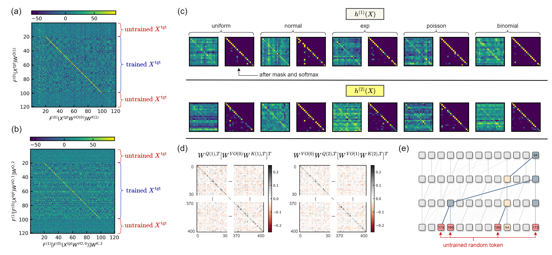
Figure 4: (a) The matching matrix $h^{(1)}(X^{\text{tgt}})$. The diagonal elements exhibit the largest values, confirming the matching operation. Note that $X^{\text{tgt}}_{0\sim 20}$ and $X^{\text{tgt}}_{100\sim 120}$ correspond to untrained tokens initialized from a random normal distribution. (b) The matching matrix $h^{(2)}(X^{\text{tgt}})$. (c) Matching matrix $h^{(1)}(X)$ and $h^{(2)}(X)$ for untrained tokens with different random initialization methods. The maximum diagonal property holds for all cases, indicating the model’s generalization ability. (d) $Ker^{(1)}=W^{Q(1),\mathsf{T}}W^{K(1)}W^{VO(0),\mathsf{T}}$ and $Ker^{(2)}=W^{VO(1)}W^{Q(2),\mathsf{T}}W^{K(2)}W^{VO(0),\mathsf{T}}$ behave like a noisy identity matrix. (e) Performance on the sequence contains untrained tokens.

Properties of Matching Matrix. We discover that even for untrained random tokens (the 0-20 and 100-120 portions in Fig. 4(a)), $h^{(1)}(X)$ can still maintain the maximum diagonal property. These tokens can be sampled from arbitrary distributions (Fig. 4(c)). As a result, even if we replace the tokens in the sequence with untrained random tokens, the model can still obtain the correct results (Fig. 4(e)). This phenomenon aligns with findings from studies on induction heads [15]. We observe that this is due to $Ker^{(1)}=W^{Q(1),\mathsf{T}}W^{K(1)}W^{VO(0),\mathsf{T}}$ being approximately an identity matrix (Fig. 4(d)). This "simplicity bias" endows the Transformer model with the ability to perform matching out of the data distribution[16, 17]. Furthermore, we find that for the matching matrix, the trained and untrained portions only differ by a constant factor (Appendix D Fig. 9(b)).

Layer 2-3: Information Matching. The second step of reasoning is matching the information of "[B]$W^{VO(0)}$+[C]" with the information of "[B]$W^{VO(1)}$" in the last node. Therefore, the matching matrix and simplified matching matrix for the 2nd layer can be defined as:

$$h^{(2)}(X)=\text{F}^{(1)}[\text{F}^{(0)}(X^{tgt})W^{VO(1)}]W^{Q(2),\mathsf{T}}[\text{F}^{(1)}[\text{F}^{(0)}(X^{tgt}W^{VO(0)})]W^{K(2),\mathsf{T}}]^{\mathsf{T}}.$$ (5)

$$\tilde{h}^{(2)}(X) =XW^{VO(1)}W^{Q(2),\mathsf{T}}[XW^{VO(0)}W^{K(2),\mathsf{T}}]^{\mathsf{T}}\triangleq XKer^{(2)}X^{\mathsf{T}}.$$ (6)

As shown in Fig. 4(b)(c)(d), the second layer also exhibits simplicity bias and the ability to perform matching out of the data distribution.

General Matching Matrix. More generally, for deeper Transformer models and multi-step reasoning tasks, the matching matrix for the $k$th-step reasoning is:

$$\tilde{h}^{(k)}(X)=XW^{VO(k-1)}W^{Q(k),\mathsf{T}}W^{K(k)}W^{VO(0),\mathsf{T}}X^{\mathsf{T}}.$$ (7)

4 Enhance Model’s Matching Ability

Initialization Method. We discovered that the initialization method has a significant impact on Transformer models’ ability to learn reasoning tasks. Specifically, we set the parameters to be initialized from a uniform distribution $U(-(6/m_{\text{in}})^{\gamma},(6/m_{\text{in}})^{\gamma})$, where $\gamma$ is set to $0.3$, $0.5$, and $1$, corresponding to small initialization, default initialization, and large initialization, respectively. Here, $m_{\text{in}}$ denotes the input dimension of each linear layer. As shown in Tab. 1, the model with small initialization has the best generalization on the test dataset for each type of task. For the training process, as shown in Fig. 12 (Appendix G) and Fig. 14 (Appendix H), we found that Transformer models with large initialization struggle to perform well on multi-step reasoning tasks. Transformer models with default initialization exhibit a noticeable Grokking phenomenon [18, 19] during training, while small initialization does not. Furthermore, different initialization methods cause the models to complete reasoning in distinct ways. We discuss this in detail in Appendix G.

LayerNorm Position. Two LayerNorm are considered: post-LayerNorm and pre-LayerNorm. Post-LayerNorm, which is the structure used in this paper’s model, places LayerNorm after the attention and FNN modules. Pre-LayerNorm, on the other hand, places LayerNorm before the attention and FNN modules. Detailed structure can be found in Appendix B. In our work, we found that post-LayerNorm has a significant facilitative effect on reasoning than pre-LayerNorm. Results in Tab. 1 illustrate the differences between using pre-LayerNorm and post-LayerNorm.

Dataset		Type 1 (%)			Type 2 (%)			Type 3 (%)
$\gamma$		0.3	0.5	1	0.3	0.5	1	0.3	0.5	1
pre-LN	train	100	100	100	100	100	100	99.40	98.79	100
	test	15.84	19.33	20.09	40.87	62.7	91.6	48.69	23.56	100
post-LN	train	100	100	100	98.6	100	100	100	100	100
	test	34.75	91.97	100	40.14	43.73	99.99	99.96	99.88	100

Table 1: Comparison of initialization and LayerNorm. Training details can be found in Appendix F G and H.

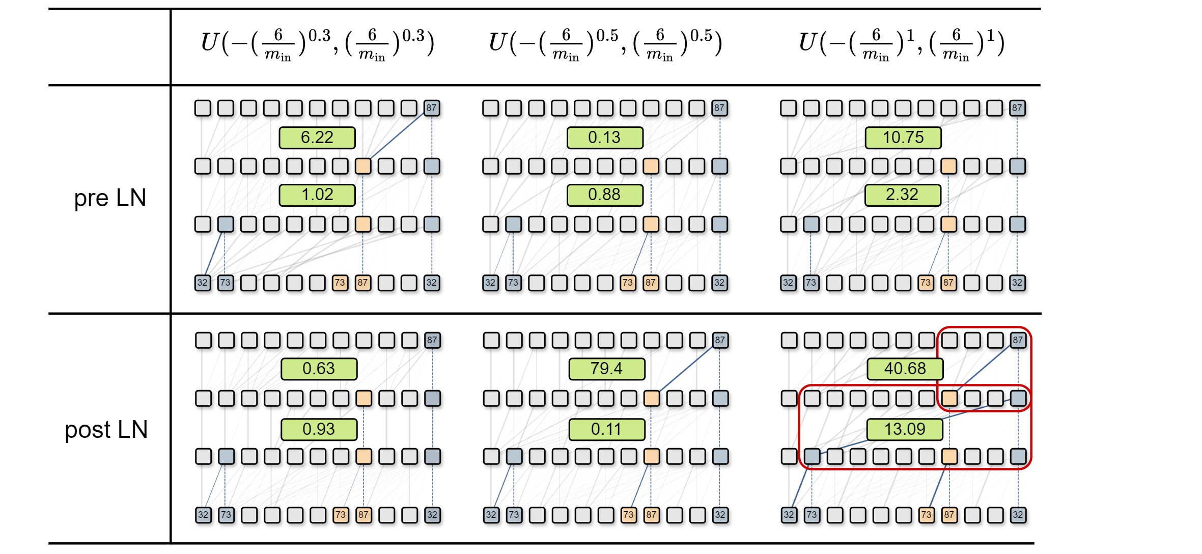
Figure 5: Comparison of the information flow and matching scores of Transformers with different initialization and LayerNorm on a training sequence. The model with small initialization and post-LayerNorm exhibits high matching scores in both layers.

Furthermore, based on the matching matrix, we define a metric called matching score ($S_{\text{m}}$) to characterize the matching ability of each layer, which is defined as:

$$S_{\text{m}}^{(l)}=\mathbb{E}_{X\sim\mathcal{N}(0,1)}\frac{\text{mean}(\text{Tr}(h^{(l)}(X)))}{\text{mean}(h^{(l)}(X)-\text{mean}(\text{Tr}(h^{(l)}(X))))}.$$ (8)

As shown in Fig. 5, we calculate the performance of Transformers with different settings on a training sequence of the Type 1 data and compute the matching score for each layer. The results indicate that the Transformer with small initialization and post-LayerNorm settings has high matching scores in both layers, suggesting that the model has strong generalization ability. In contrast, the Transformers with other settings have low matching scores in at least one layer, indicating that they rely more on memorization in the FNN layers rather than inference using the attention layers to complete the reasoning tasks, making it difficult to achieve generalization.

In Appendix E, we further calculate the matching score for each head in a real-world language model, Phi-3 [20], and test the model’s performance on a reasoning task similar to the Type 3 data. The results reveal that the model’s reasoning approach is highly correlated with the matching score of each layer, and the information propagation process closely resembles the information flow diagram of Transformers on the Type 3 data (Fig. 15, Appendix H).

Add Orthogonal Noise. To maximize the diagonal elements of the matching matrices $\tilde{h}^{(1)}(X)$ and $\tilde{h}^{(2)}(X)$, we need to make $W^{Q(1),\mathsf{T}}W^{K(1)}W^{VO(0),\mathsf{T}}$ and $W^{VO(1)}W^{Q(2),\mathsf{T}}W^{K(2)}W^{VO(0),\mathsf{T}}$ closer to identity matrices. Boix-Adsera et al. [15] demonstrated that replacing $W^{Q,\mathsf{T}}W^{K}$ and $W^{VO}$ with $W^{Q,\mathsf{T}}W^{K}+\alpha I$ and $W^{VO}+\beta I$ can improve the induction capability of the model. However, under this setting, the attention matrix may face the problem of degeneration. We observed that $W^{Q,\mathsf{T}}W^{K}$ does not necessarily possess the property of maximum diagonal elements (Fig. 9(e) Appendix D). Therefore, we choose to replace $W^{Q(l),\mathsf{T}}W^{K(l)}$ and $W^{VO(l)}$ with $W^{Q(l),\mathsf{T}}W^{K(l)}+\alpha^{(l)}Z$, and $W^{VO(l)}+\beta^{(l)}Z^{\mathsf{T}}$, respectively, where $\alpha^{(l)}$ and $\beta^{(l)}$ are learnable parameters, and $Z\in\mathbb{R}^{d_{m}\times d_{m}}$ is a random matrix following $N(0,1)$. Fig. 6 demonstrates the performance of the improved model on Type 1 data. Details can be found in Appendix I.

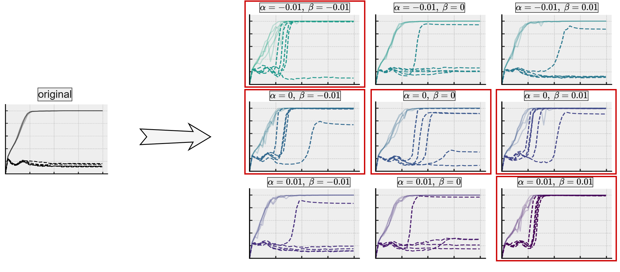
Figure 6: The impact of different learnable parameters’ initial values, $\alpha^{(l)}$ and $\beta^{(l)}$, on the model’s reasoning ability. When $\alpha^{(l)}_{\text{ini}}=0$ or $\alpha^{(l)}$ and $\beta^{(l)}$ have the same sign initially, the model’s reasoning capability can be enhanced. The solid lines represent the training accuracy, while the dashed lines denote the test accuracy. Each experiment was conducted with five random seeds.

5 Mechanism of Parallel Reasoning and Upper Bound Conjecture

Mechanism of Parallel Reasoning. Fig. 7(a) illustrates the information flow of a 4-layer model completing 4-step reasoning. We observe that when the reasoning steps exceed or equal the number of model layers, the model performs multiple matching operations parallelly in one layer. In the 2nd layer, different information undergoes two matching operations, enabling the subsequent three layers to achieve 4-step reasoning. Moreover, starting from the 2nd layer, the model’s matching approach transits from matching tokens’ values to matching tokens’ positions. Token value matching is only utilized in the 1st layer.

Based on the mechanism of information propagation, at the $l$-th layer, if the information is transmitted through attention, it should be multiplied by a coefficient $W^{VO(l)}$, whereas no such term is required if it is transmitted through residual connections. Consequently, in Fig. 7(c), we present the coefficients by which each information is multiplied. It is observed that for each positional information, the coefficients are distinct, and the same holds true for the value information. The variation in coefficients also indicates that the information is stored in different subspaces, thereby enabling parallel reasoning.

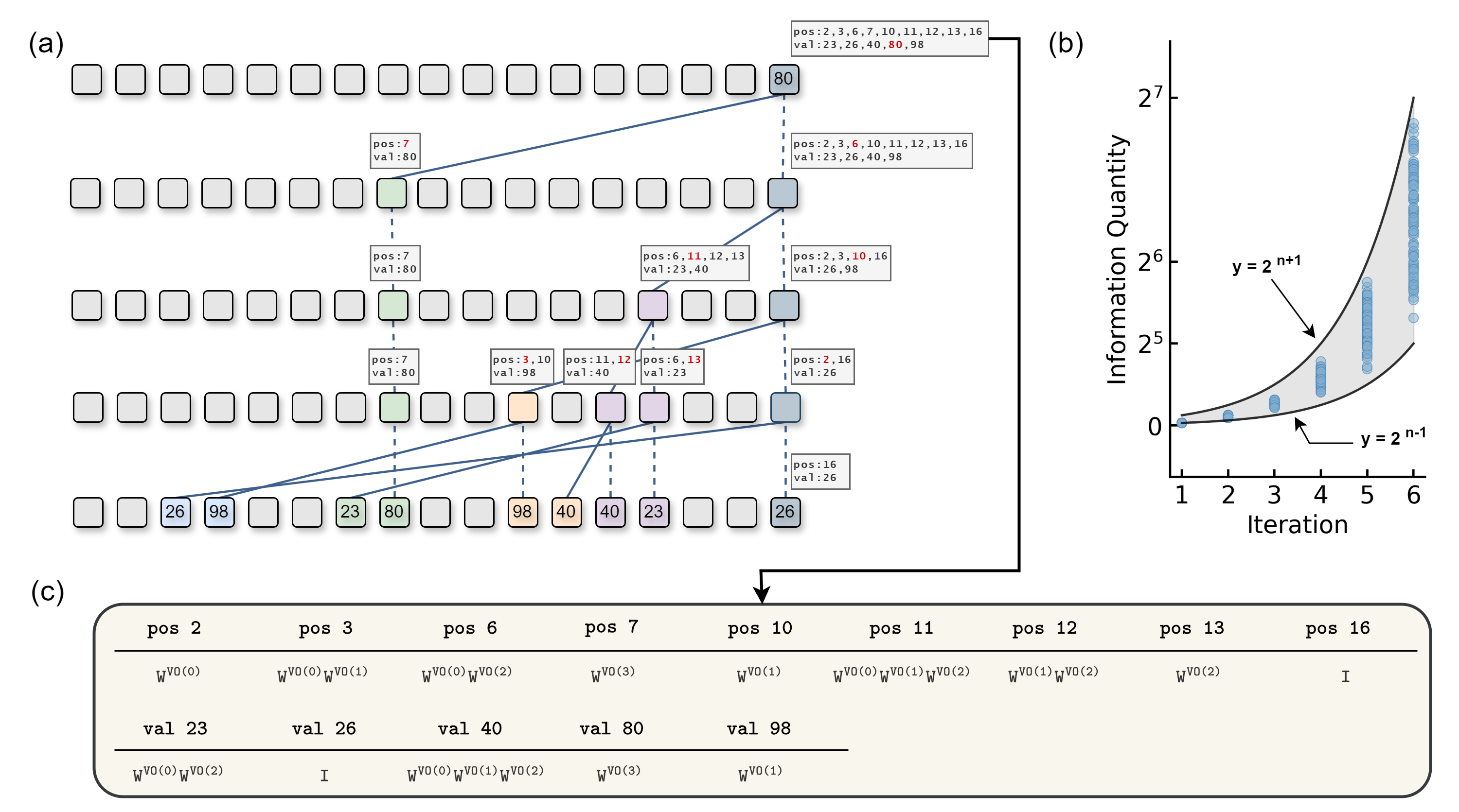
Figure 7: (a) Information flow of a 4-layer Transformer model completing 4-step reasoning. (b) Number of stored information tokens in the last position with respect to the number of iterations when propagating information based on the Info-Prop Rules. We randomly selected 1000 sentences for the simulation. The blue dots represent the simulation results. (c) The coefficients by which each information is multiplied.

Upper Bound of Model’s Reasoning Ability. Through the study of the matching mechanism in Transformer models, we can estimate the upper bound of the reasoning ability for a general L-layer Transformer network. First, we assume that the model satisfies the following assumption.

Assumption 1

Assume that the hidden space dimension $d_{m}$ is sufficiently large, allowing different information to be stored in independent subspaces without interference. Moreover, information transmission is achieved solely through the matching operation of the Attention module, without considering the influence of the FNN module.

We regard $n$ tokens of a sequence as $n$ nodes, each storing position and value information. The Transformer model follows the Information Propagation (Info-Prop) Rules (denoting the node transmitting information as $i$ and the node receiving information as $j$, considering the existence of the attention mask, we require $i$ < $j$):

• Rule 1: Odd positions can pass information to subsequent even positions, i.e., node $i$ stores an odd number $a$ in its position information, and node $j$ stores $a+1$ in its position information.

• Rule 2: The position information stored in node $i$ and node $j$ has common elements.

• Rule 3: The value information stored in node $i$ and node $j$ has common elements.

If any of the above three rules are satisfied, we consider that the information from node $i$ can be transmitted to node $j$. When information transmission occurs, the position and value information stored in node $j$ will take the union of the corresponding information from node $i$ and node $j$.

Pseudocode 1 (Appendix J) provides a detailed process of the Info-Prop Rules. Fig. 7(b) shows the number of value information stored in the last token with respect to the number of iterations under our set of rules. It can be observed that the stored information exhibits an approximately exponential growth pattern with the number of iterations. Fig. 19 (Appendix J) discusses the minimum number of steps required to transmit the final reasoning result to the last token. Based on these results, we propose the following conjecture:

Conjecture 1 (Upper Bound of Transformer’s Reasoning Ability)

Under the premise of Assumption 1, in the L-th layer, the subspaces of the hidden space for value information and position information can only be divided through $\{\prod_{l\in J}W^{VO(l)}|J\subset\{0,1,\cdots,L-1\}\}$. Therefore, the maximum amount of information in the last layer is $2^{L+1}$. Considering the influence of the mask, the upper bound of the model’s reasoning ability is $2^{L-1}\sim 2^{L+1}$.

However, in practice, the hidden space dimensions $d_{m}$, $d_{q}$, $d_{k}$, and $d_{v}$ of large language models are far from meeting the requirements of Assumption 1. Consequently, the actual reasoning ability of large language models is also constrained by the hidden space dimensions. On the other hand, due to the presence of FNN and other attention mechanisms, the model’s ability to integrate various types of information is further enhanced. Therefore, considering all factors, we believe that the reasoning ability of Transformers lies between linear and exponential growth.

6 Related Work

In-Context Learning and Induction Head The concept of in-context learning (ICL) was first introduced by Brown et al. [7]. Since then, a series of studies have utilized induction heads to investigate ICL, yielding remarkable research outcomes [12, 21, 22, 23, 24, 25, 26, 27, 28]. It is worth noting that induction heads can be considered as a special case of multi-step reasoning tasks, where the reasoning step is limited to 1. However, multi-step reasoning is not a simple linear combination of single-step reasoning. In this work, we study the matching mechanism that enables multi-step reasoning and the phenomenon of parallel reasoning, which have not been explored in previous studies.

Initialization and Layernorm Initialization is a crucial factor influencing model performance. Different initialization settings can lead to various network states, such as linear behavior under large initialization[29, 30, 31, 32, 33] and condensation phenomenon under small initialization [34, 35]. Researchers have also explored the use of different initialization techniques to improve the stability of large models [36, 37, 38]. Zhang et al. [39] suggests that large initialization tends to memorize, while small initialization tends to learn inference. LayerNorm [40] is a widely used normalization technique in Transformer models, which has been shown to improve the stability and performance of deep neural networks. Studies have investigated the effect of LayerNorm on the training dynamics, generalization, and gradient flow in Transformers [41, 42]. The use of LayerNorm in conjunction with different initialization techniques has also been explored to enhance the training stability of Transformers [38].

Attention Mechanism Our work builds upon previous studies on the attention mechanism [43, 44, 45, 46]. Numerous researchers have proposed various approaches to identify the roles of different heads in Transformers [47, 48, 21, 49, 50]. These methods predominantly employ the concept of perturbation. As a complementary approach, we propose a direct computation method to identify heads with matching functionality. Similar to the observations made by Wang et al. [51] and Dutta et al. [52], who noted that large language models typically perform information aggregation in shallow layers and information induction in deeper layers, we have also observed comparable phenomena in our study. Our idea of constructing language-like datasets is inspired by Poli et al. [53], Zhang et al. [54].

7 Discussion

Conclusion. In this work, by designing rigorous datasets and analyzing the model’s internal information flow, we uncovered the crucial role of the matching operation in enabling multi-step reasoning. We proposed the concept of a matching matrix to quantify the model’s matching ability and explored factors that influence this ability. Furthermore, we investigated the relationship between model depth and reasoning capability, revealing the potential for parallel reasoning in Transformers and proposing a conjecture on the upper bound of their reasoning ability.

Limitations and Future Work. Our analysis focused on Transformer models with a single attention head, which allowed us to simplify the problem and gain a clear understanding of the matching operation. However, most Transformer models employ multi-head attention mechanisms, and the dynamics of multi-step reasoning in these networks may involve more complex interactions between different attention heads. Further research is needed to extend our analysis to multi-head attention networks and explore the theoretical implications of our conjecture on the upper bound of the reasoning ability of Transformers.

Appendix A Notations and Transformer Structure

In this section, we give the notation of the transformer in modules to facilitate subsequent analysis of its mechanism. The notation we used in this work is same as Zhang et al. [54].

Input Representation. The input sequence is represented as a one-hot vector $X^{\mathrm{in}}\in\mathbb{R}^{n\times d}$, where $n$ is the sequence length, $d$ is the dictionary size, and $X^{\mathrm{in}}$ is the one-hot vector.

After embedding, the input sequence becomes:

$$X^{\mathrm{tgt}}=X^{\mathrm{in}}W^{\mathrm{em}}\in\mathbb{R}^{n\times d_{m}},\quad W^{\mathrm{em}}\in\mathbb{R}^{d\times d_{m}}.$$

The positional vector is denoted as:

$$X^{\mathrm{pos}}\in\mathbb{R}^{n\times d_{m}}.$$

The input to the first transformer block is:

$$X^{(1)}=X^{\mathrm{tgt}}+X^{\mathrm{pos}}.$$

Single Head Self-Attention. For the $l$-th layer, the $Q,K,V$ matrices of the attention mechanism are defined as functions of the input $X^{(l)}\in\mathbb{R}^{n\times d_{m}}$:

$$Q^{(l)}(X^{(l)})=X^{(l)}W^{Q(l),\mathsf{T}},\quad W^{Q(l)}\in\mathbb{R}^{d_{q}\times d_{m}}$$

$$K^{(l)}(X^{(l)})=X^{(l)}W^{K(l),\mathsf{T}},\quad W^{K(l)}\in\mathbb{R}^{d_{k}\times d_{m}}$$

$$V^{(l)}(X^{(l)})=X^{(l)}W^{V(l),\mathsf{T}},\quad W^{V(l)}\in\mathbb{R}^{d_{v}\times d_{m}}$$

The attention matrix $\mathrm{Attn}^{(l)}(X^{(l)})$ for the $l$-th layer is computed as:

$$\mathrm{Attn}^{(l)}(X^{(l)})=\text{softmax}\left(\frac{\text{mask}({Q^{(l)}(X^{(l)})K^{(l)}(X^{(l)})^{\mathsf{T}}})}{\sqrt{d_{k}}}\right)\in\mathbb{R}^{n\times n},$$

where the function $\text{softmax}(\cdot)$ is defined as:

$$\text{softmax}(\bm{x})_{i}=\frac{e^{x_{i}}}{\sum_{j=1}^{k}e^{x_{j}}},$$

The output of the attention mechanism, denoted as $X^{\mathrm{qkv}(l)}$, is given by:

$$X^{\mathrm{qkv}(l)}=\mathrm{Attn}^{(l)}(X^{(l)})V^{(l)}(X^{(l)})\in\mathbb{R}^{n\times d_{k}}.$$

Finally, the output after position-wise feedforward processing is obtained using residual connection and layer normalization:

$$X^{\mathrm{pr}(l)}=X^{\mathrm{qkv}(l)}W^{O(l),\mathsf{T}},\quad W^{O(l)}\in\mathbb{R}^{d_{m}\times d_{v}},\quad X^{\mathrm{pr}(l)}\in\mathbb{R}^{n\times d_{m}}.$$

The output of the $l$-th layer, $X^{\mathrm{ao}(l)}$, is computed as:

$$X^{\mathrm{ao}(l)}=\text{LayerNorm}(X^{(l)}+X^{\mathrm{pr}(l)}).$$

Feedforward Neural Network (FNN). The $l$-th layer Feedforward Neural Network (FNN) is expressed as:

$$X^{\mathrm{do}(l)}:=\text{FNN}(X^{\mathrm{ao}(l)})=\text{LayerNorm}\left(X^{\mathrm{ao}(l)}+\sigma(X^{\mathrm{ao}(l)}W^{l,1})W^{l,2}\right),$$

where $\sigma(\cdot)=\text{ReLU}(\cdot)$, and $W^{l,1}\in\mathbb{R}^{d_{m}\times 3d_{m}}$, $W^{l,2}\in\mathbb{R}^{3d_{m}\times d_{m}}$.

Projection Layer. The projection layer is defined as:

$$Y=X^{\mathrm{do}(L)}W^{\mathrm{proj}}+b^{\mathrm{proj}},\quad W^{\mathrm{proj}}\in\mathbb{R}^{d_{m}\times d},\quad b^{\mathrm{proj}}\in\mathbb{R}^{d},\quad Y\in\mathbb{R}^{n\times d}.$$

The output is obtained by taking the argmax of the softmax:

$$\text{Output}=\text{argmax}(\text{softmax}(Y)).$$

Appendix B Post LayerNorm and Pre LayerNorm Structure

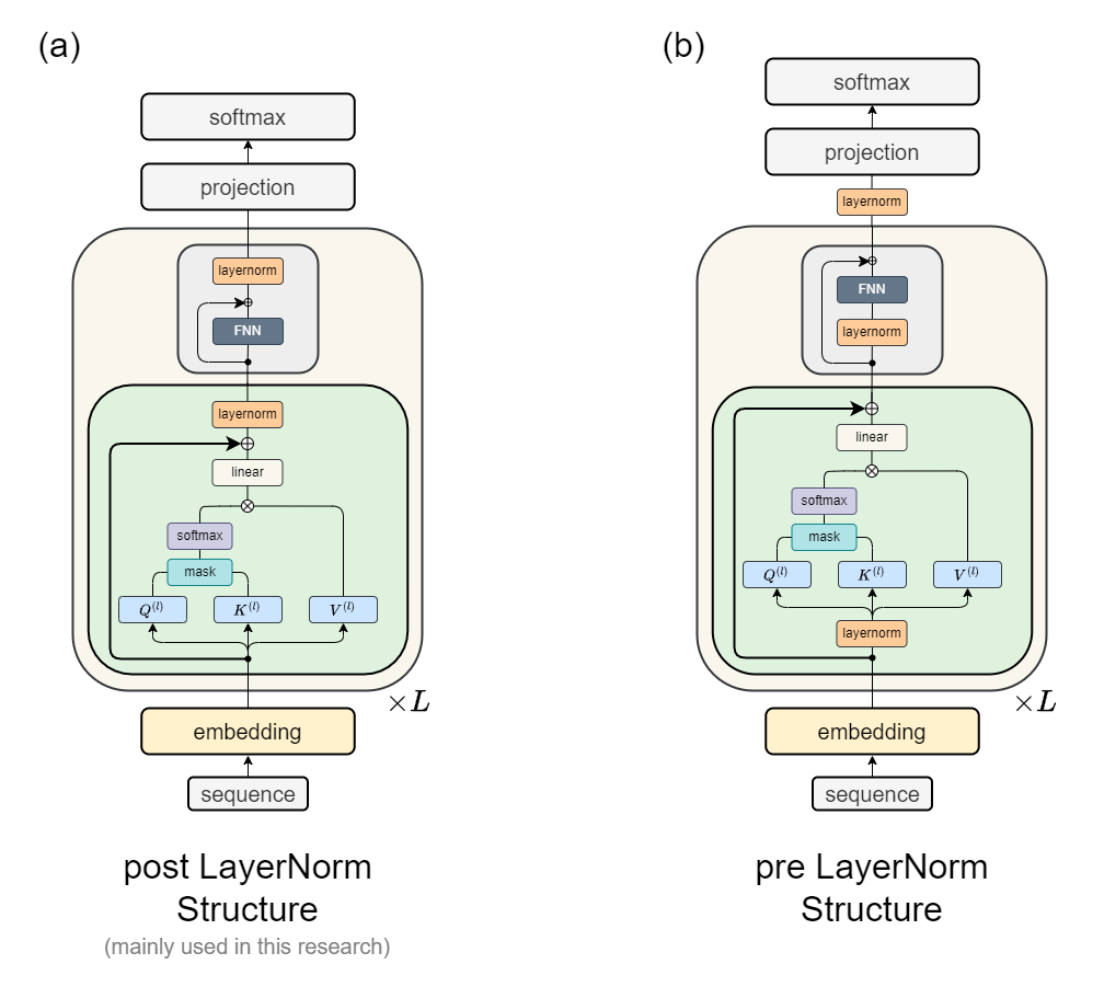
Figure 8: Transformer structure we used in this research. (a) post LayerNorm structure (mainly used). (b) pre LayerNorm structure.

Appendix C Experimental settings

In our experiments, unless otherwise specified, we use the post-LayerNorm decoder-only Transformer architecture shown in Fig. 8(a). The vocabulary size is set to $d=201$, and during training, all tokens x are restricted to the range of [20, 100]. We set the hidden space dimension to $d_{m}=400$ and $d_{q}=d_{k}=d_{v}=64$.

For training, we use a batch size of 100 and the AdamW optimizer with default parameters as set in PyTorch 2.3.0. The learning rate strategy is either a fixed value or a combination of GradualWarmupScheduler and CosineAnnealingLR. We employ a gradient clipping strategy with torch.nn.utils.clip_grad_norm_(model.parameters(), max_norm=1).

The experiments were conducted on a server with the following configuration:

• 64 AMD EPYC 7742 64-Core Processor.

• 256GB of total system memory.

• 2 NVIDIA A100 GPUs with 40GB of video memory each and 8 NVIDIA GeForce RTX 4080 GPUs with 16GB of video memory each.

• The experiments were run using Ubuntu 22.04 LTS operating system.

The task shown in Appendix D can be completed within 2 hours using a single NVIDIA A100 GPU. For other more complex examples, they can be finished within 24 hours.

Appendix D Experimental settings and Property of Matching Operation

Settings. We use 200,000 2-step reasoning chains (13-length single chain structure) with a fixed learning rate of 2e-5 and a batch size of 100. The 3-layer Transformer model is trained for 200 epochs and reaches 100% train and test accuracy.

Mechanism of Positional Embedding. Positional encoding plays a major role in the attention module of the first layer. Fig. 9(a) shows the positional attention matrix computed as follows:

$$\mathrm{Attn}^{\text{pos}(1)}=\mathrm{softmax}\left(\frac{\mathrm{mask}(X^{\text{pos}}W^{Q(l),\mathsf{T}}W^{K(l)}X^{\text{pos},\mathsf{T}})}{\sqrt{d_{k}}}\right)$$ (9)

Matching Matrix. For the matching matrix $h^{(1)}(X)$, we find that the model can maintain the diagonal element property in most cases, even for untrained random embedding vectors. Further analysis of the matching matrices obtained from trained and untrained embedding vectors reveals that they differ by an almost constant factor. As shown in Fig. 9(b), multiplying $h^{(1)}(X^{\text{tgt}}_{20\sim 100})$ by a constant factor of 0.5 yields results nearly identical to $h^{(1)}(X^{\text{tgt}}_{0\sim 20})$ (where the vector $X^{\text{tgt}}_{0\sim 20}$ is untrained). .

Simplified Matching Matrix. Moreover, we discover that although the Transformer contains FNN and LayerNorm layers, their impact on the matching mechanism is minimal. Fig. 9(c)(d) shows the simplified version of the matching matrix $\tilde{h}^{(1)}(X)$ and $\tilde{h}^{(2)}(X)$ obtained by removing all FNN and LayerNorm layers. We find that it also exhibits the maximum diagonal property, indicating that the matching operation is primarily implemented by the self-attention module.

Property of $W^{Q(1),\mathsf{T}}W^{K(1)}$. As shown in Fig.9(e), we observe that it exhibits a random matrix pattern without any apparent structure. In contrast, the matrix $Ker^{(1)}=W^{Q(1),\mathsf{T}}W^{K(1)}W^{VO(0)}$ defined in Eq.4 of the main text exhibits a noisy identity matrix pattern (Fig. 4(d)). This suggests that $W^{VO(0),\mathsf{T}}$ is approximately equal to $W^{Q(1),\mathsf{T}}W^{K(1)}$. The benefit of this arrangement is that it allows for the matching operation to be performed without imposing additional constraints on the $W^{Q(1)}$ and $W^{K(1)}$ matrices, enabling them to adapt to other tasks as well.

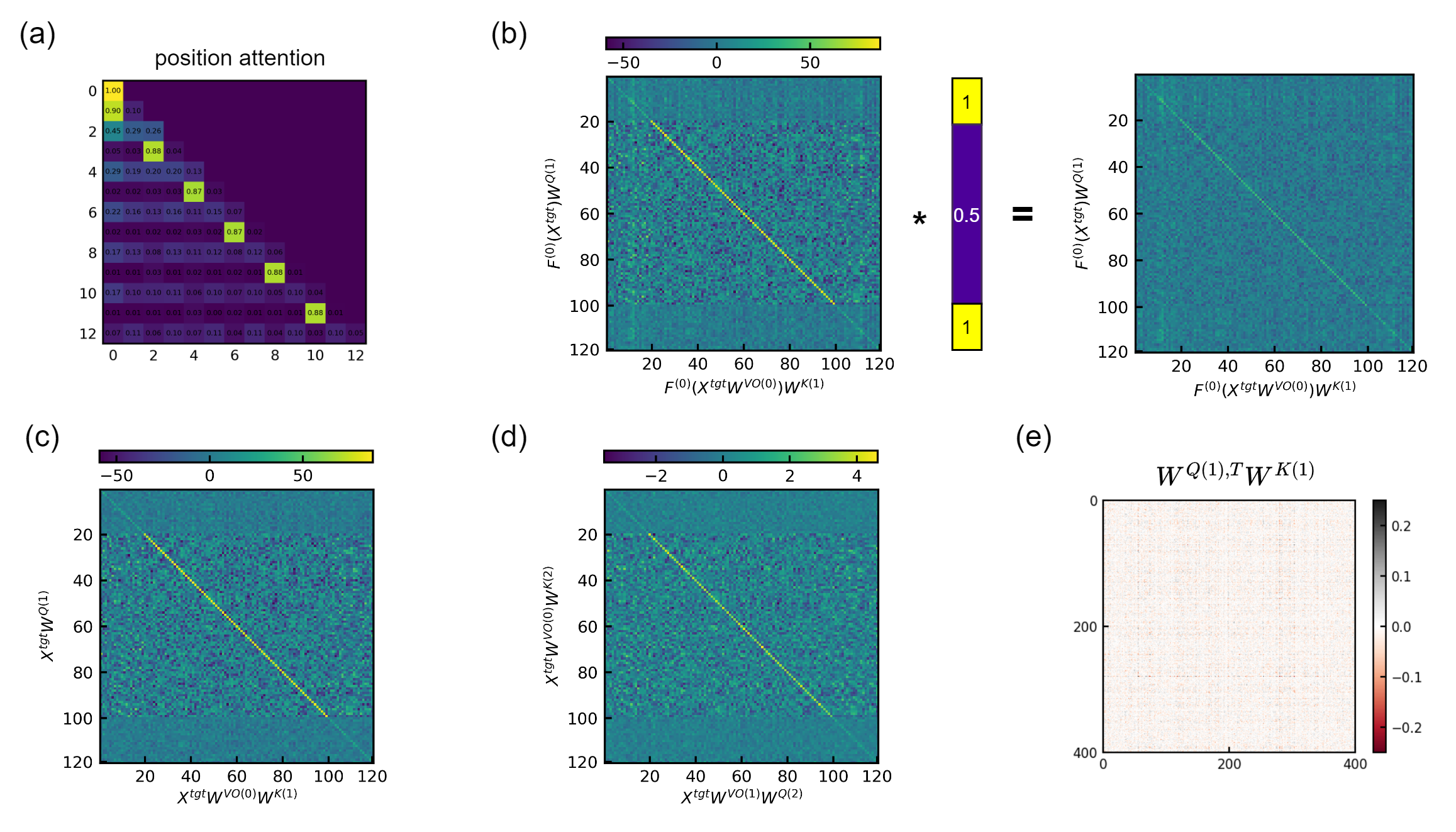
Figure 9: (a) Visualization of $\mathrm{Attn}^{\text{pos}(1)}$. (b) Multiplying $h^{(1)}(X^{\text{tgt}}_{20\sim 100})$ (trained) by a constant factor of 0.5 yields results nearly identical to $h^{(1)}(X^{\text{tgt}}_{0\sim 20})$ (untrained). (c)(d) Visualization of the simplified matching matrix $\tilde{h}^{(1)}(X^{tgt})$ and $\tilde{h}^{(2)}(X^{tgt})$. The diagonal elements exhibit the largest values, confirming the matching operation. (e) Visualization of the $W^{Q(1),\mathsf{T}}W^{K(1)}$ matrix, which exhibits a random matrix pattern without any apparent structure.

Appendix E Matching Phenomenon in LLM

We tested the matching score of the large language model phi-3 and observed how it performs a 2-step reasoning task. In the main text, we defined the matching score for a single-head Transformer. For phi-3, which has a multi-head and pre-LayerNorm structure, we can calculate the matching matrix of the $h$-th head in the $l$-th layer as follows:

$$X^{\text{vo}} =\text{LN}^{(l-1)}_{\text{attn}}(X)W^{V(l-1),\mathsf{T}}W^{O(l-1),\mathsf{T}}$$ (10)

$$X^{\text{vof}} =X^{\text{vo}}+\text{FNN}^{(l-1)}(\text{LN}^{(l-1)}_{\text{FNN}}(X^{\text{vo}}))$$ (11)

$$X^{\text{vok},h} =\text{LN}^{(l)}_{\text{attn}}(X^{\text{vof}})W^{K(l,h)}$$ (12)

$$X^{\text{f}} =\text{LN}^{(l-1)}_{\text{attn}}(X)+\text{FNN}^{(l-1)}(\text{LN}^{(l-1)}_{\text{FNN}}(\text{LN}^{(l-1)}_{\text{attn}}(X)))$$ (13)

$$X^{\text{q},h} =X^{\text{f}}W^{Q(l,h)}$$ (14)

$$\text{matching matrix: }h^{(l,h)} =X^{\text{q},h}X^{\text{vok},h,\mathsf{T}}.$$ (15)

We visualized the matching score of each head in each layer (Fig. 10(a)) and found that the matching scores were highest in layers 5 to 20. For the 2-step reasoning task shown in Fig. 10(b), we observed its attention matrix and roughly constructed the information transmission path for each piece of information. We discovered that its reasoning process is similar to the information flow shown in Fig. 15(e), and this reasoning process is completed within layers 5 to 20.

However, it is worth noting that the sub-equation (10) shown above cannot accurately reflect the information propagation process in the same way as the single-head attention structure. For multi-head models, a more precise method of calculating the matching score requires further research.

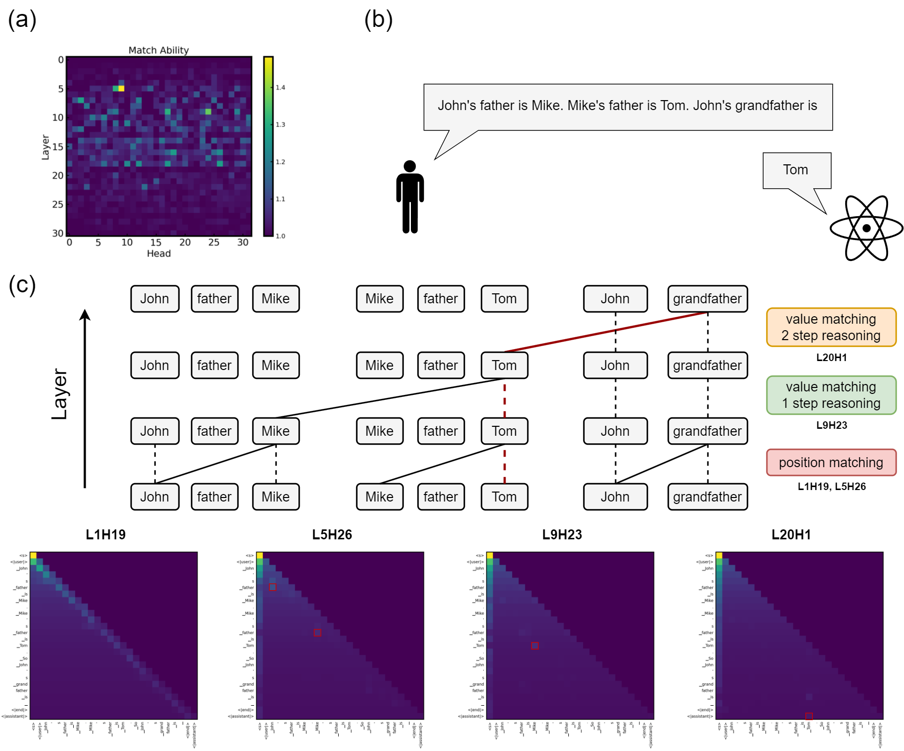
Figure 10: Multi-step reasoning example with Phi-3 language model.

Appendix F Details for Training Type1 Dataset

Settings and Results. This section provides supplementary details on the experimental setup for the Transformer learning the Type 1 dataset. In all three experiments, we use a 3-layer Transformer network with 1 attention head per layer, where $d_{q}=d_{k}=d_{v}=64$ and $d_{m}=400$. The training set consists of 300,000 single reasoning chains with a sequence length of 11. The learning rate starts at 5e-5, increases to 2e-4 within 100 epochs, and gradually decreases to 1e-5. The AdamW optimizer is used. For these three experiments, we set the uniform sampling interval of parameter initialization to $(6/m_{\text{in}})^{0.3}$ (large initialization), $(6/m_{\text{in}})^{0.5}$ (default initialization), and $(6/m_{\text{in}})^{1}$ (small initialization). Fig. 11 shows the loss and accuracy during the training process.

(a) Loss, pre-LayerNorm

(b) Loss, post-LayerNorm

(c) Accuracy, pre-LayerNorm

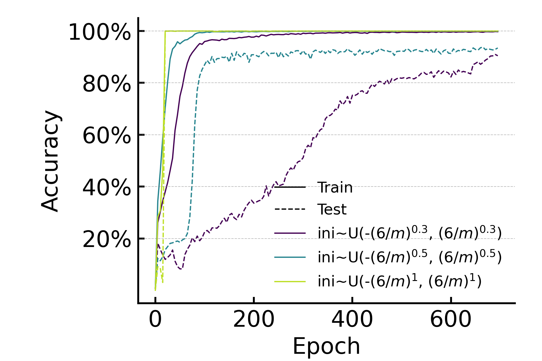
(d) Accuracy, post-LayerNorm

Figure 11: Performance on type1 2-step reasoning dataset.

Appendix G Details for Training Type2 Dataset

Settings and Results. This section provides supplementary details on the experimental setup for the Transformer learning the Type 2 dataset. In all three experiments, we use a 5-layer Transformer network with 1 attention head per layer, where $d_{q}=d_{k}=d_{v}=64$ and $d_{m}=400$. The training set consists of 300,000 reasoning chains with a sequence length of 17, and an equal number of 1-step, 2-step, and 3-step reasoning chains. The learning rate starts at 5e-5, increases to 2e-4 within 200 epochs, and gradually decreases to 1e-5. The AdamW optimizer is used. We consider the uniform sampling interval of parameter initialization to $(6/m_{\text{in}})^{0.3}$ (large initialization), $(6/m_{\text{in}})^{0.5}$ (default initialization), and $(6/m_{\text{in}})^{1}$ (small initialization). Fig. 12 shows the changes in loss and accuracy with respect to epochs during the training process. Fig. 13 presents the information flow of the model’s reasoning.

Infomation Flow Analysis. Fig. 13 illustrates the similarities and differences in the information flow of post-LayerNorm Transformer models with default and small initialization when performing 1-step, 2-step, and 3-step reasoning on the same sequence after training. Both models process the sequence by fusing information from odd and even positions in the first layer and then performing one-step reasoning in each subsequent layer.

However, we observed that the default initialization tends to perform broadcasting operations when not performing reasoning, propagating the information of the token at the first position to all subsequent positions. This results in the information at subsequent positions in the next layer being in the form of "[token₀]$W^{VO}$+[res]". Since the magnitude of $W^{VO}$ is O(1) under default initialization, after multiple rounds of broadcasting, the information at subsequent positions becomes almost equal to the information of [token₀], causing the attention matrix from layer 4 to layer 5 to degenerate into an "averaged" matrix. This may lead to information loss and hinder further training of higher-step reasoning tasks, such as 4-step reasoning.

In contrast, small initialization tends to continue performing the same matching operation as the previous layer after reaching the end of the reasoning chain. This is because the residual connection plays a dominant role under small initialization. For a reasoning chain "$\texttt{[}\texttt{a}_{1}\texttt{]}\rightarrow\texttt{[}\texttt{a}_{2}\texttt{]}\rightarrow\texttt{[}\texttt{a}_{3}\texttt{]}\dashrightarrow\texttt{[}\texttt{a}_{4}\texttt{]}$", assuming after 3-step reasoning, the last column in layer $l$ is "$\texttt{[}\texttt{a}_{3}\texttt{]}W^{VO(l-1)}$", its query should have the largest inner product with the key of "$\texttt{[}\texttt{a}_{3}\texttt{]}W^{VO(0)}+\texttt{[}\texttt{a}_{4}\texttt{]}$", followed by the second largest inner product with the key of "$\texttt{[}\texttt{a}_{2}]W^{VO(0)}+\texttt{[}\texttt{a}_{3}\texttt{]}$". Therefore, when "$\texttt{[a}_{4}\texttt{]}$" does not exist in the sequence, it will continue to recognize the term "$\texttt{[}\texttt{a}_{2}\texttt{]}W^{VO(0)}+\texttt{[}\texttt{a}_{3}\texttt{]}$" and propagate "$\texttt{[}\texttt{a}_{3}\texttt{]}W^{VO(l-1)}$" to the end. This mechanism facilitates further training of more complex reasoning tasks: when training a higher-step (e.g., 4-step) reasoning task, only slight adjustments to the parameters of the last layer are needed to ensure that

$$(\texttt{[}\texttt{a}_{3}\texttt{]}W^{VO(l-1)})W^{Q(l)}W^{K(l),\mathsf{T}}(\texttt{[}\texttt{a}_{3}\texttt{]}W^{VO(0)})^{\mathsf{T}}>(\texttt{[}\texttt{a}_{3}\texttt{]}W^{VO(l-1)})W^{Q(l)}W^{K(l),\mathsf{T}}(\texttt{[}\texttt{a}_{3}\texttt{]})^{\mathsf{T}}.$$

Figure 12: Type2 1-3 steps reasoning loss and accuracy.

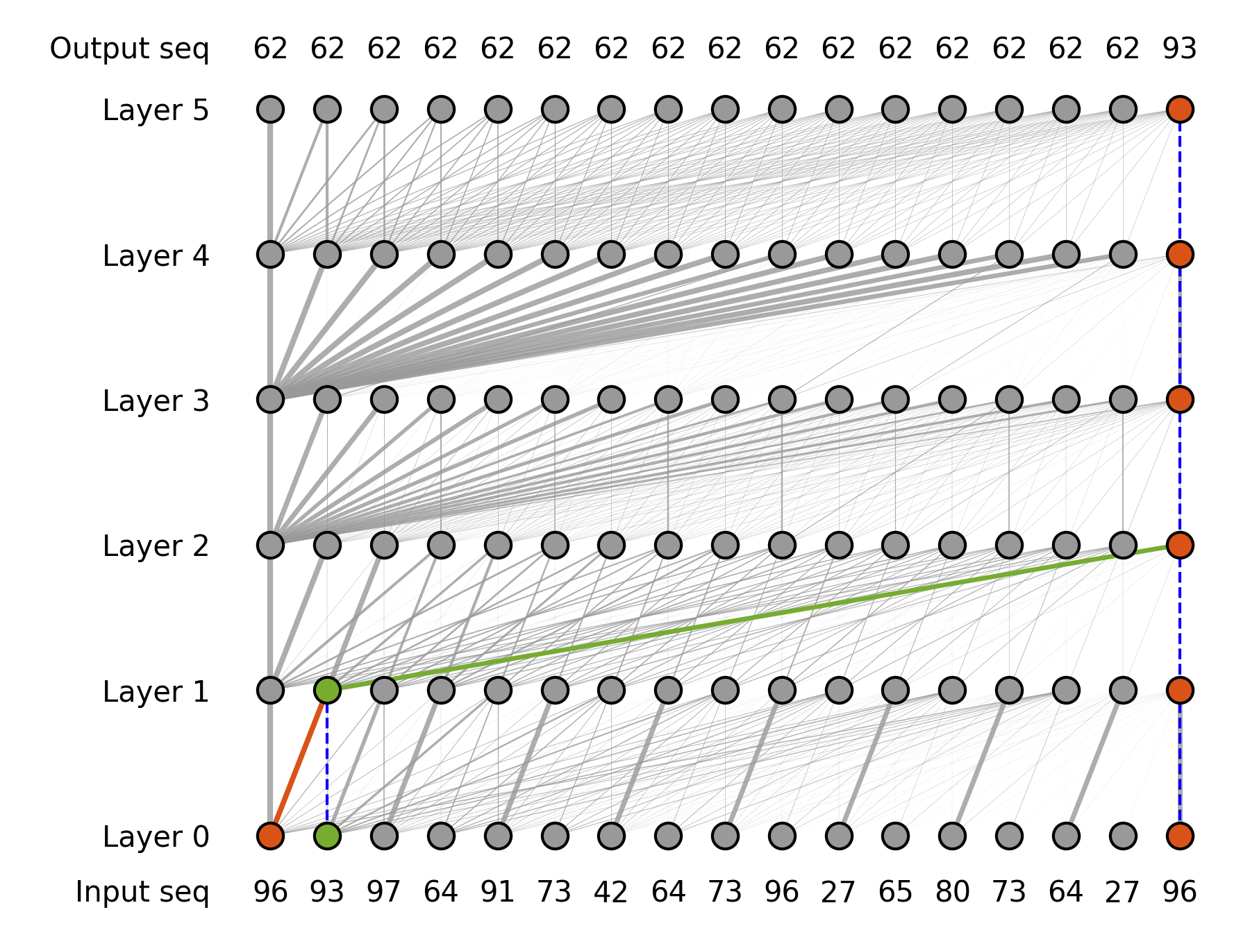
(a) 1-step, default initial

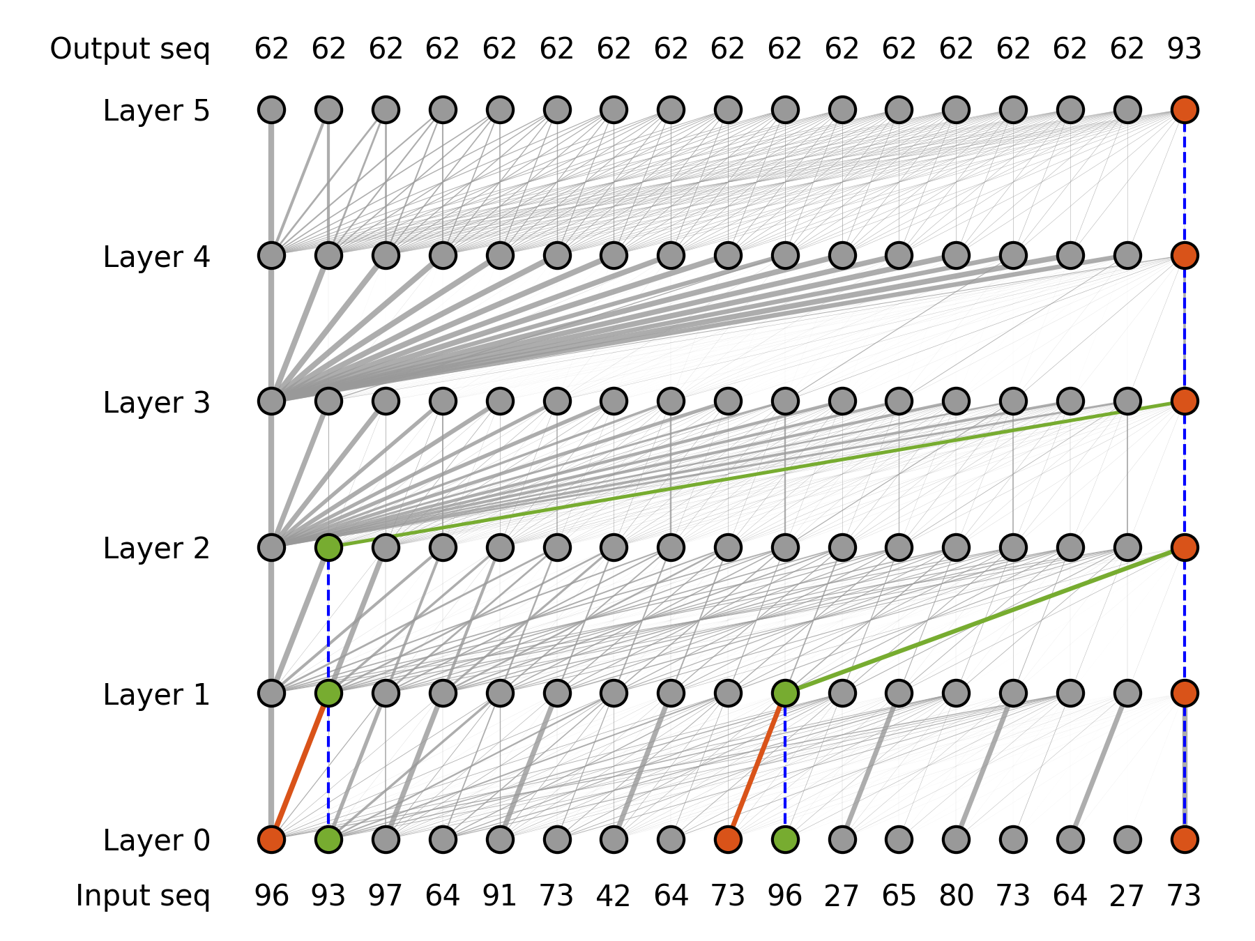
(b) 2-step, default initial

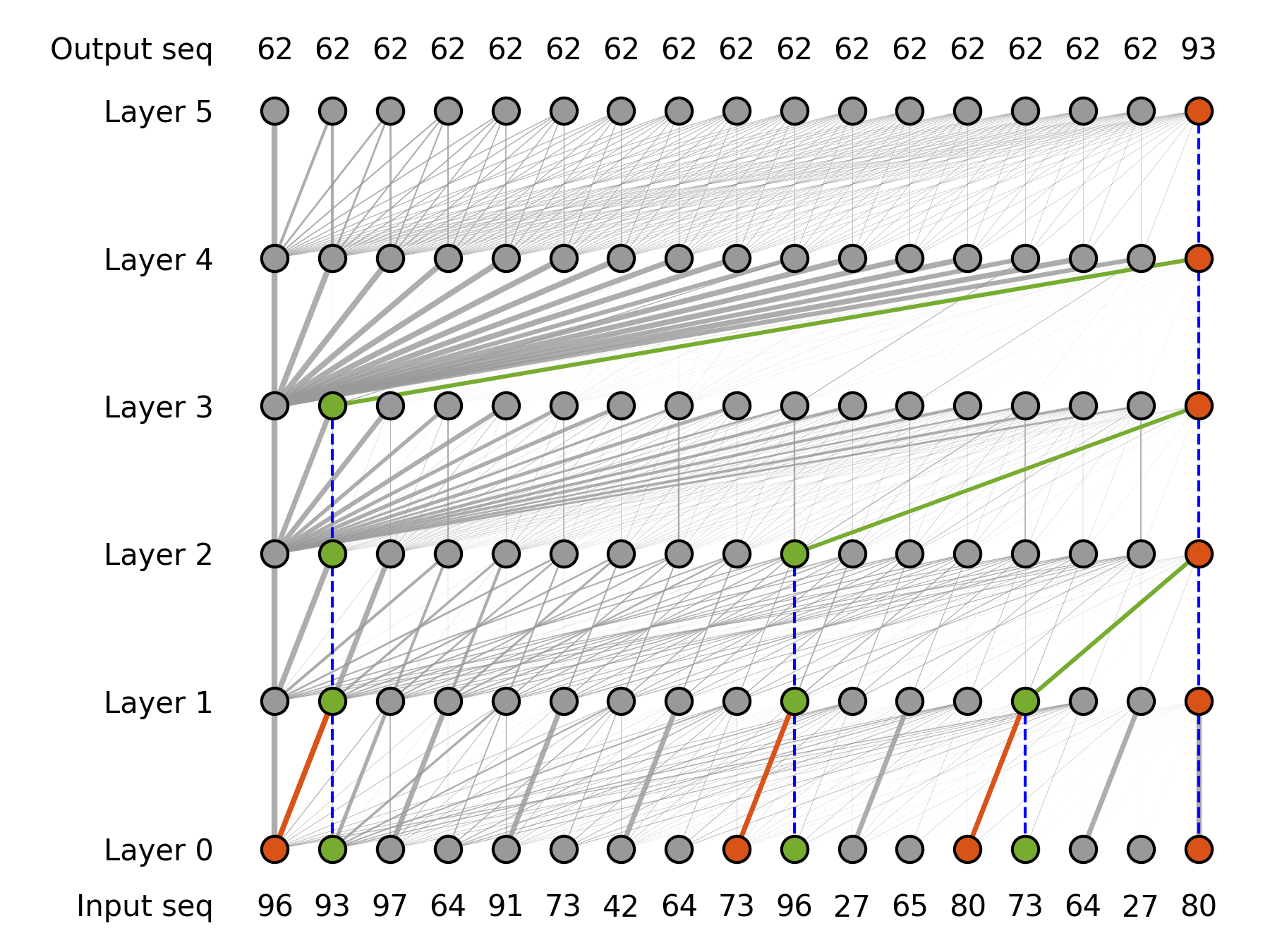
(c) 3-step, default initial

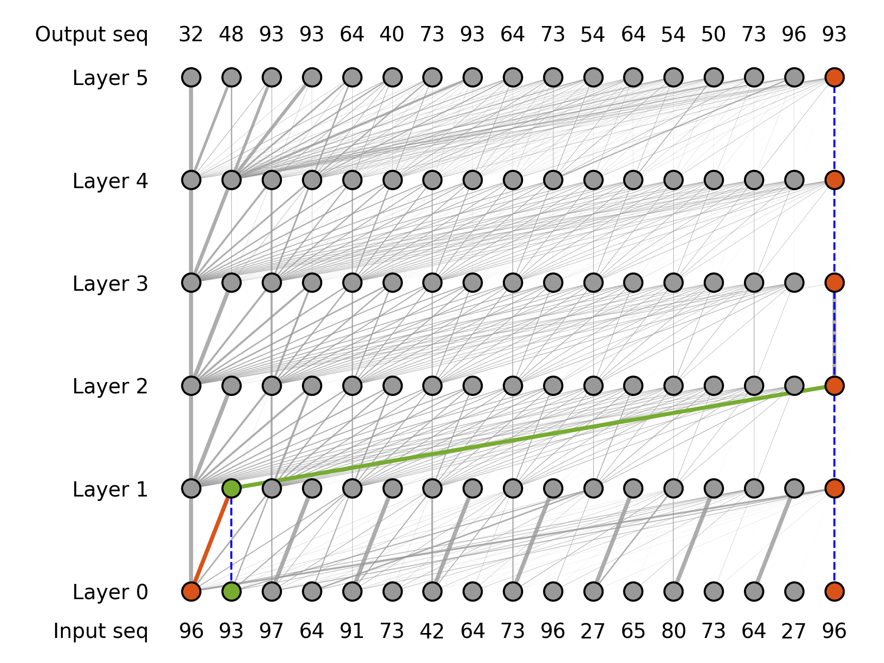
(d) 1-step reasoning, small initial

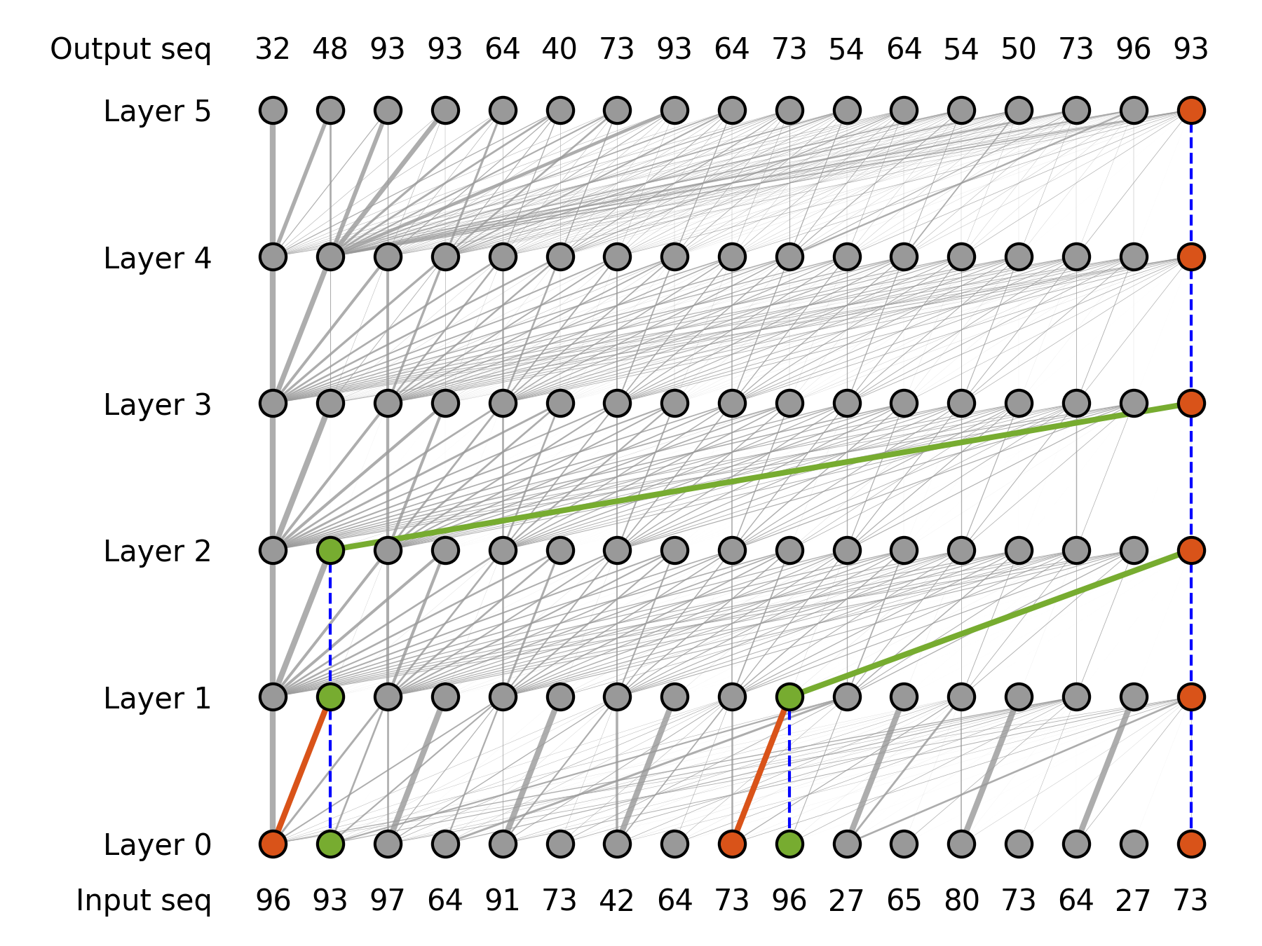
(e) 2-step reasoning, small initial

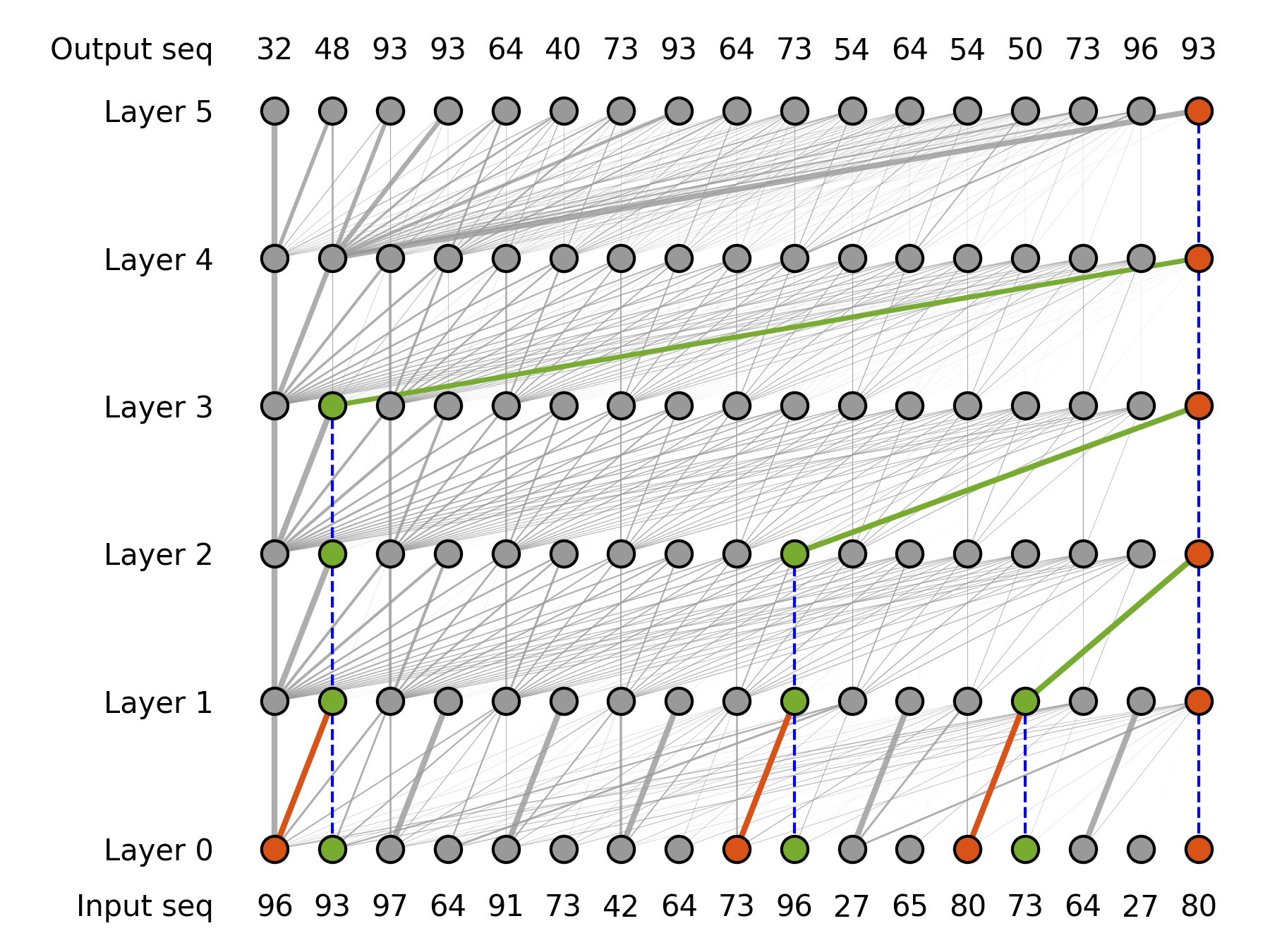
(f) 3-step reasoning, small initial

Figure 13: Performance on type3 1-3 steps reasoning dataset.

Appendix H Details for Training Type3 Dataset

Settings and Results. This section provides supplementary details on the experimental setup for the Transformer learning the Type 3 dataset. In all three experiments, we use a 5-layer Transformer network with 1 attention head per layer, where $d_{q}=d_{k}=d_{v}=64$ and $d_{m}=400$. The training set consists of 300,000 reasoning chains with a sequence length of 13, and an equal number of 1-step, 2-step, and 3-step reasoning chains. The learning rate starts at 5e-5, increases to 2e-4 within 200 epochs, and gradually decreases to 1e-5. The AdamW optimizer is used. For these three experiments, we set the uniform sampling interval of parameter initialization to $(6/m_{\text{in}})^{0.3}$ (large initialization), $(6/m_{\text{in}})^{0.5}$ (default initialization), and $(6/m_{\text{in}})^{1}$ (small initialization). Fig. 14 shows the loss and accuracy during the training process. Fig. 15 presents the information flow of the model’s reasoning.

Infomation Flow Analysis. For the information flow graphs of Type 3 data shown in Fig. 15, the models trained under the two initialization and post LayerNorm also exhibit differences in their processing of the sequence. The network trained with default initialization tends to complete the matching operation in the second-to-last column, i.e., the column containing the "start point", while the network trained with small initialization tends to complete the matching operation in the last column, i.e., the column containing the "step". Further research is needed to investigate the causes and advantages/disadvantages of these two mechanisms.

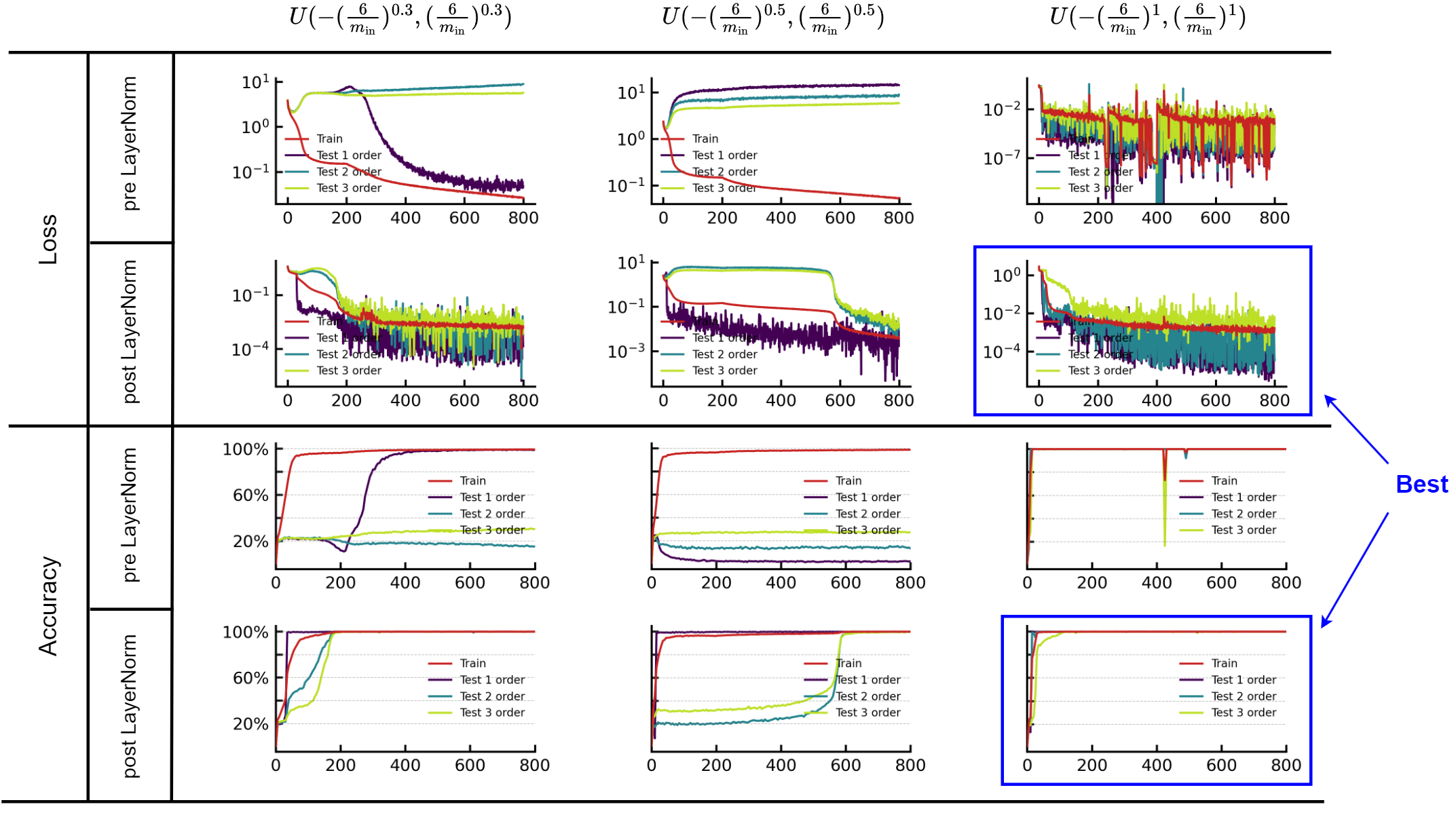
Figure 14: Type3 1-3 steps reasoning loss and accuracy.

(a) 1-step, default initial

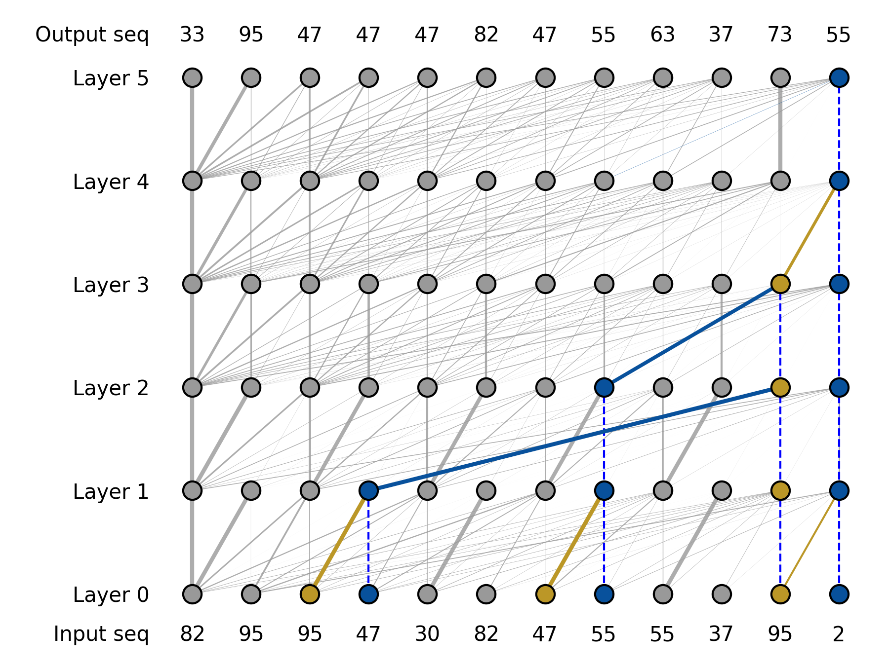
(b) 2-step, default initial

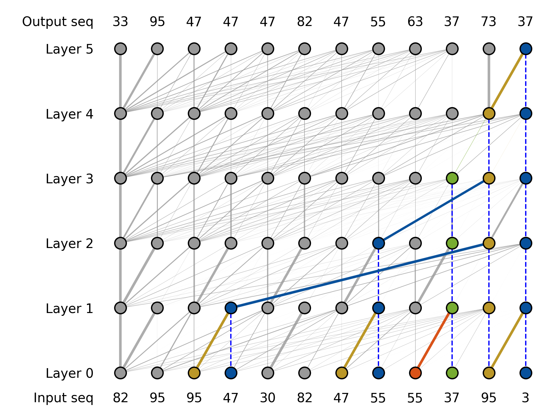
(c) 3-step, default initial

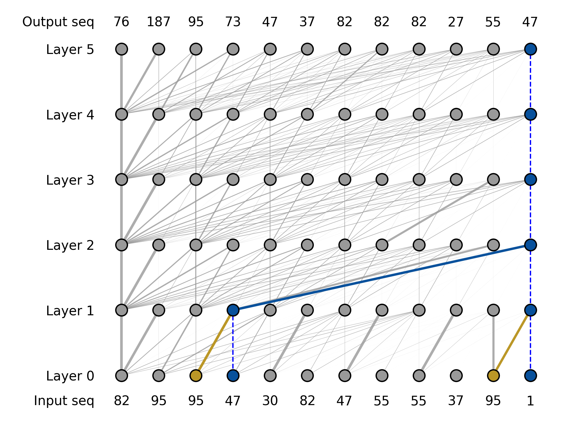
(d) 1-step, small initial

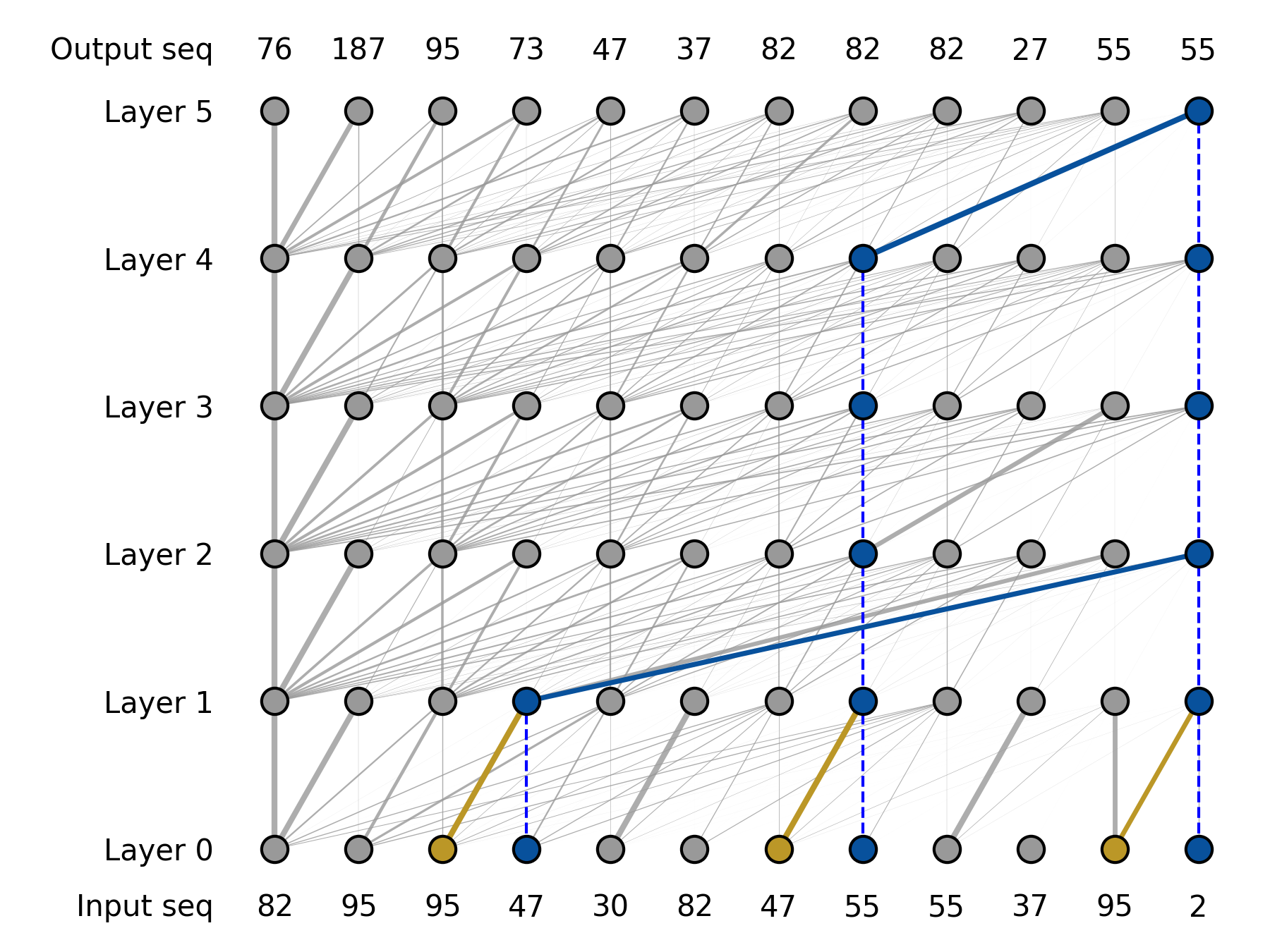
(e) 2-step, small initial

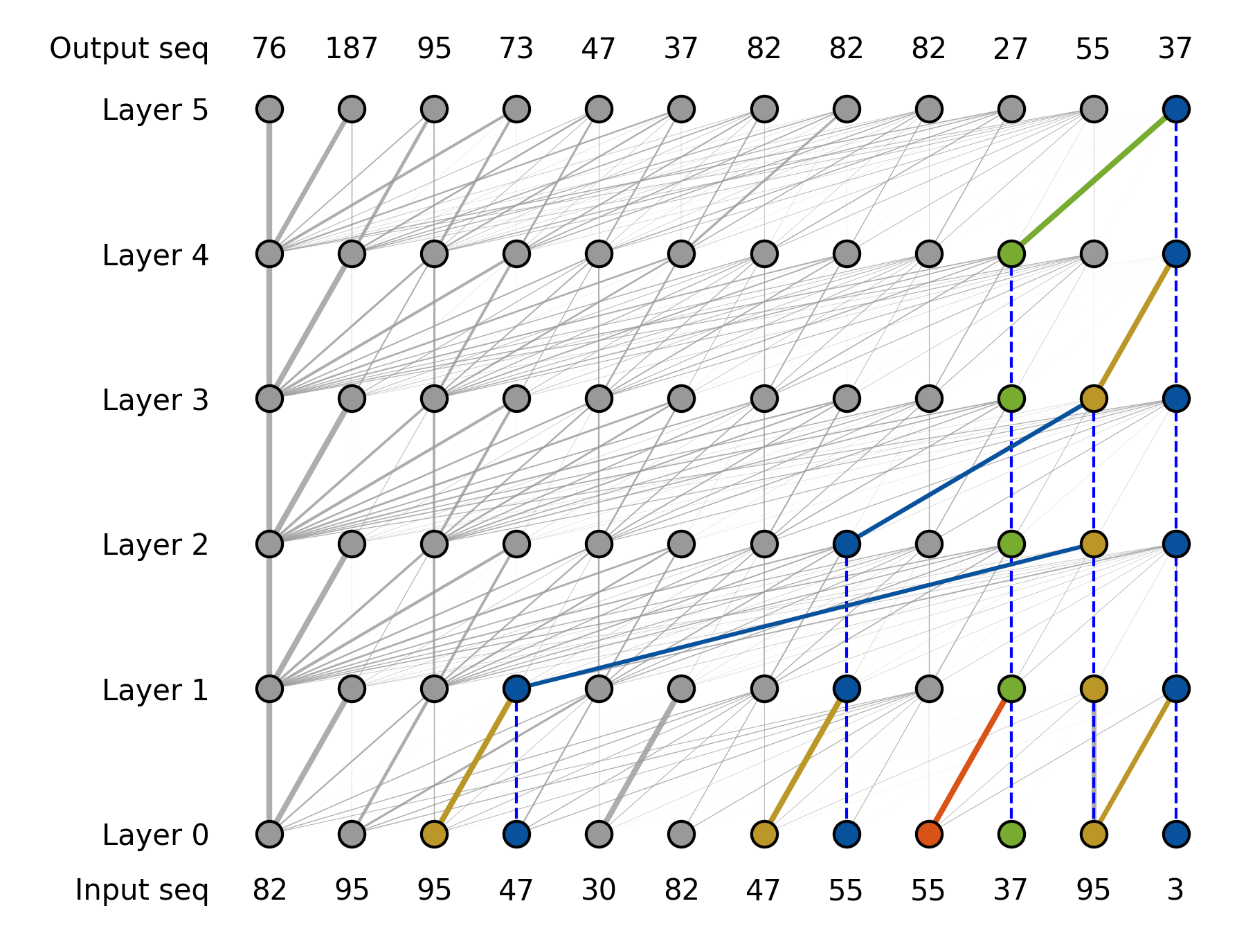
(f) 3-step, small initial

Figure 15: Performance on type3 1-3 steps reasoning dataset.

Appendix I Details for Adding Orthogonal Noise Experiment

This section provides supplementary details on the experimental setup for adding orthogonal noise experiment. We use a post-LayerNorm 3-layer Transformer network, where $d_{q}=d_{k}=d_{v}=64$ and $d_{m}=400$. The training set consists of 30,000 2-step reasoning chains (11-length single chain structure). The learning rate starts at 5e-5, increases to 2e-4 within 20 epochs, and gradually decreases to 1e-5. We trained the model for 200 epochs in total. The AdamW optimizer is used. The parameters are initialed form a uniform distribution $U(-(6/m_{\text{in}})^{0.5},(6/m_{\text{in}})^{0.5})$. In this setting, the Transformers have poor generation ability in the test dataset.

We replace $W^{Q(l),\mathsf{T}}W^{K(l)}$ and $W^{VO(l)}$ with $W^{Q(l),\mathsf{T}}W^{K(l)}+\alpha^{(l)}Z$, and $W^{VO(l)}+\beta^{(l)}Z^{\mathsf{T}}$, respectively, where $\alpha^{(l)}$ and $\beta^{(l)}$ are learnable parameters, and $Z\in\mathbb{R}^{d_{m}\times d_{m}}$ is a random matrix following $N(0,1)$. Therefore, 6 extra learnable parameters are added to this 3-layer single-head model in total. Fig. 16 and Fig. 17 show the loss and accuracy of the Transformer under different settings. Fig. 18 shows the changes of the learnable parameters $\alpha^{(l)}$ and $\beta^{(l)}$ during training.

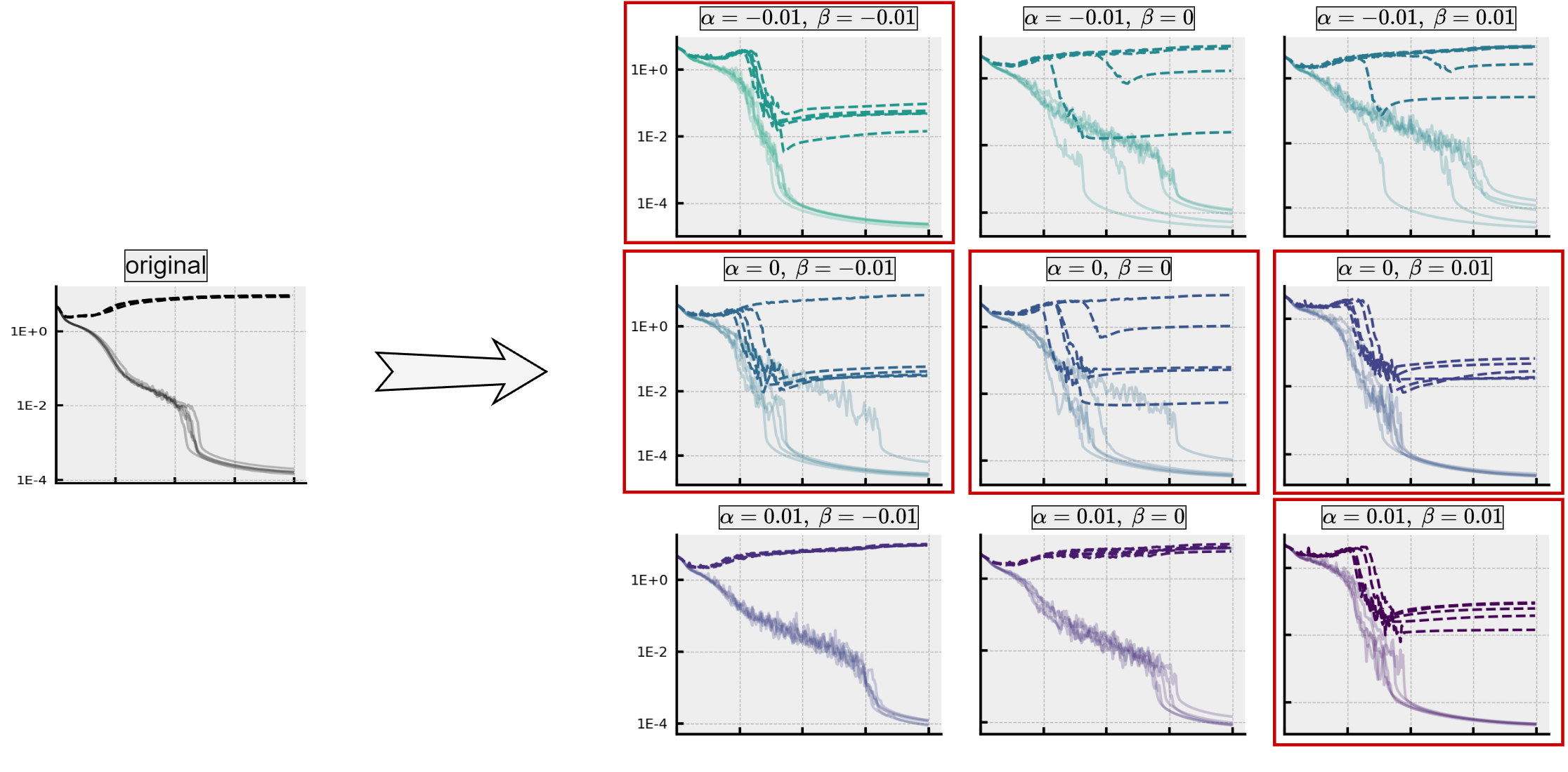
Figure 16: The impact of different learnable parameters’ initial values, $\alpha^{(l)}$ and $\beta^{(l)}$, on the model’s reasoning ability. The solid lines represent the training loss, while the dashed lines denote the test loss. Each experiment was conducted with five random seeds.

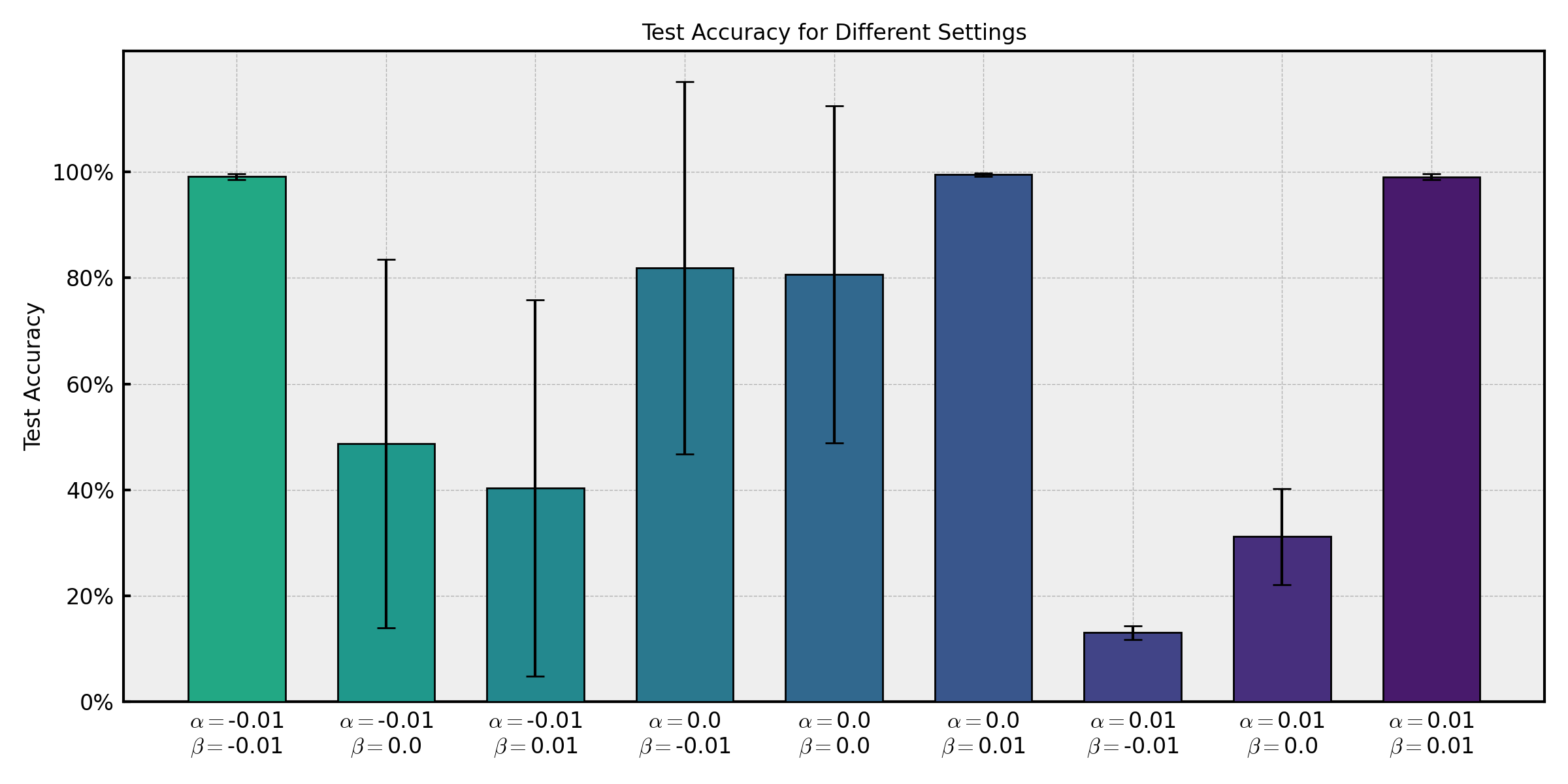
Figure 17: The average accuracy of different initial value of $\alpha^{(l)}$ and $\beta^{(l)}$.

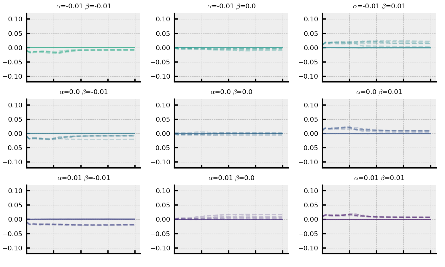
(a) layer 0

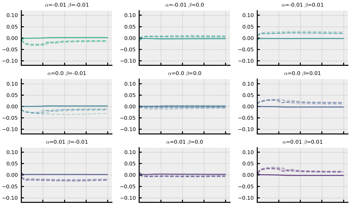
(b) layer 1

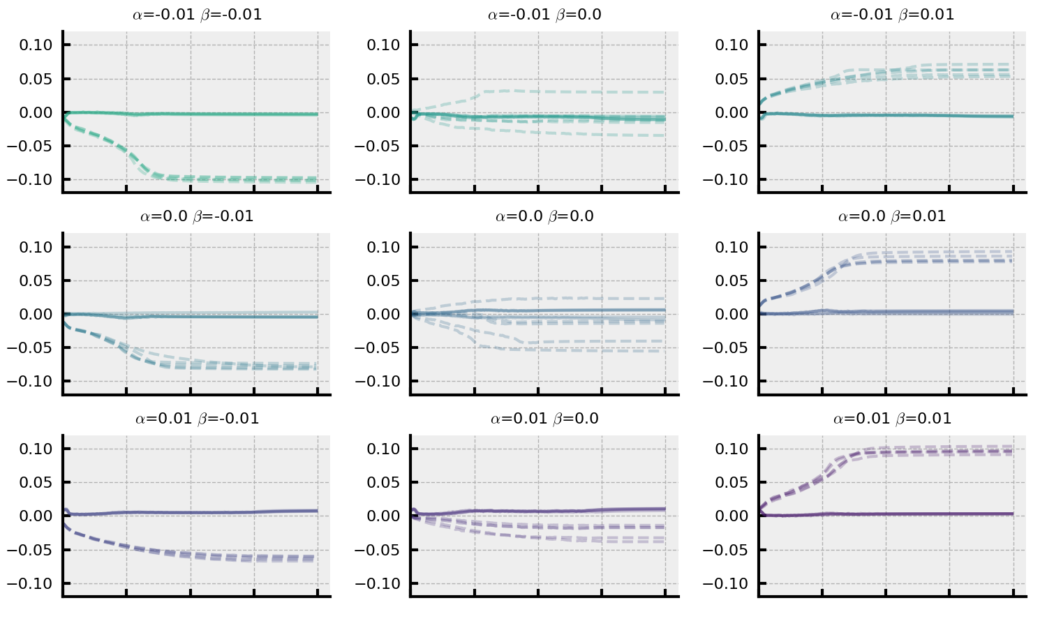
(c) layer 2

Figure 18: Changes of the learnable parameters $\alpha^{(l)}$ and $\beta^{(l)}$ during training.The solid lines represent the $\alpha^{(l)}$, while the dashed lines denote the $\beta^{(l)}$. Each experiment was conducted with five random seeds.

Appendix J Pseudocode for Upper Bound of Reasoning Ability

Pseudocode 1 shows the implementation process of the Info-Prop Rules mentioned in the main text. Each Node[i] is a dictionary containing two attributes: pos (position) and val (value). Node[i][pos] and Node[i][val] are two sets. Initially, each set contains only its own information and will be updated according to the Info-Prop Rules.

Algorithm 1 Information Propagation Rules

1:  Initialize an empty dictionary Node

2:  for each token i in the sequence do

3:     Node[i][pos] $\leftarrow$ i

4:     Node[i][val] $\leftarrow$ token i

5:  end for

6:  Node_new $\leftarrow$ Node

7:  Information propagation

8:  for each node i in Node do

9:     for each node j > i in Node do

10:        rule1 $\leftarrow$ any even number $a\in$ Node[i][pos] satisfies $a+1\in$ Node[j][pos]

11:        rule2 $\leftarrow$ Node[i][val] $\cap$ Node[j][val] $\neq\varnothing$

12:        rule3 $\leftarrow$ Node[i][pos] $\cap$ Node[j][pos] $\neq\varnothing$

13:        if rule1 or rule2 or rule3 then

14:           Node_new[j][pos] $\leftarrow$ Node_new[j][pos] $\cup$ Node[i][pos]

15:           Node_new[j][val] $\leftarrow$ Node_new[j][val] $\cup$ Node[i][val]

16:        end if

17:     end for

18:  end for

Figure 19 discusses the minimum number of steps required to transmit the final reasoning result to the last token.

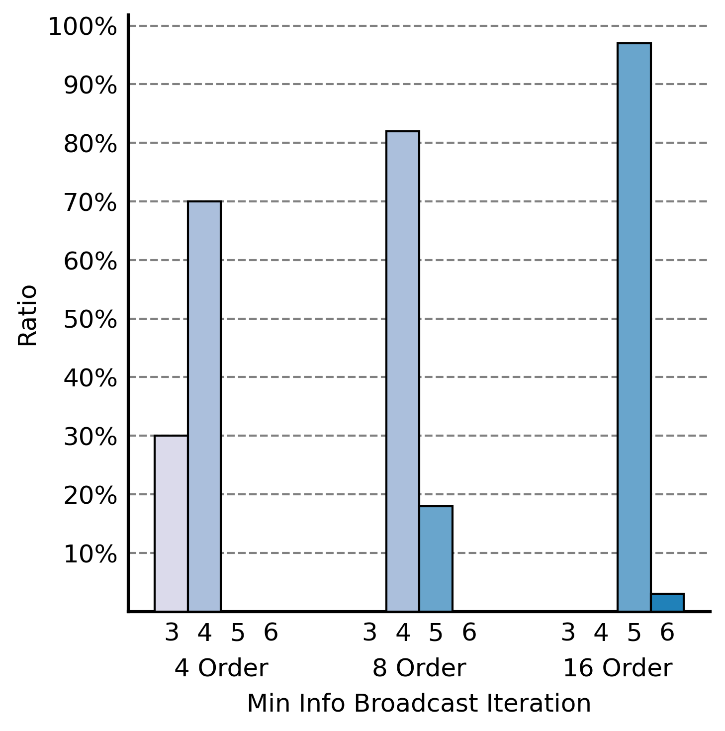
Figure 19: Minimum number of iterations required to transmit the labels of different steps of reasoning to the last position when propagating information based on the Info-Prop Rules.

References

- Vaswani et al. [2017] A. Vaswani, N. Shazeer, N. Parmar, J. Uszkoreit, L. Jones, A. N. Gomez, Ł. Kaiser, I. Polosukhin, Attention is all you need, Advances in neural information processing systems 30 (2017).
- Liu et al. [2018] P. J. Liu, M. Saleh, E. Pot, B. Goodrich, R. Sepassi, L. Kaiser, N. Shazeer, Generating wikipedia by summarizing long sequences, arXiv preprint arXiv:1801.10198 (2018).
- Devlin et al. [2018] J. Devlin, M.-W. Chang, K. Lee, K. Toutanova, Bert: Pre-training of deep bidirectional transformers for language understanding, arXiv preprint arXiv:1810.04805 (2018).
- Radford et al. [2019] A. Radford, J. Wu, R. Child, D. Luan, D. Amodei, I. Sutskever, Language models are unsupervised multitask learners (2019).
- Touvron et al. [2023] H. Touvron, T. Lavril, G. Izacard, X. Martinet, M.-A. Lachaux, T. Lacroix, B. Rozière, N. Goyal, E. Hambro, F. Azhar, et al., Llama: Open and efficient foundation language models, arXiv preprint arXiv:2302.13971 (2023).
- OpenAI [2023] OpenAI, Gpt-4 technical report, 2023. arXiv:2303.08774.
- Brown et al. [2020] T. Brown, B. Mann, N. Ryder, M. Subbiah, J. D. Kaplan, P. Dhariwal, A. Neelakantan, P. Shyam, G. Sastry, A. Askell, et al., Language models are few-shot learners, Advances in neural information processing systems 33 (2020) 1877–1901.
- Dong et al. [2022] Q. Dong, L. Li, D. Dai, C. Zheng, Z. Wu, B. Chang, X. Sun, J. Xu, Z. Sui, A survey on in-context learning, arXiv preprint arXiv:2301.00234 (2022).
- Garg et al. [2022] S. Garg, D. Tsipras, P. S. Liang, G. Valiant, What can transformers learn in-context? a case study of simple function classes, Advances in Neural Information Processing Systems 35 (2022) 30583–30598.
- Trinh et al. [2024] T. H. Trinh, Y. Wu, Q. V. Le, H. He, T. Luong, Solving olympiad geometry without human demonstrations, Nature 625 (2024) 476–482.
- Davies et al. [2021] A. Davies, P. Veličković, L. Buesing, S. Blackwell, D. Zheng, N. Tomašev, R. Tanburn, P. Battaglia, C. Blundell, A. Juhász, et al., Advancing mathematics by guiding human intuition with ai, Nature 600 (2021) 70–74.
- Olsson et al. [2022] C. Olsson, N. Elhage, N. Nanda, N. Joseph, N. DasSarma, T. Henighan, B. Mann, A. Askell, Y. Bai, A. Chen, et al., In-context learning and induction heads, arXiv preprint arXiv:2209.11895 (2022).
- Wei et al. [2022] J. Wei, X. Wang, D. Schuurmans, M. Bosma, F. Xia, E. Chi, Q. V. Le, D. Zhou, et al., Chain-of-thought prompting elicits reasoning in large language models, Advances in neural information processing systems 35 (2022) 24824–24837.
- Kojima et al. [2022] T. Kojima, S. S. Gu, M. Reid, Y. Matsuo, Y. Iwasawa, Large language models are zero-shot reasoners, Advances in neural information processing systems 35 (2022) 22199–22213.
- Boix-Adsera et al. [2023] E. Boix-Adsera, O. Saremi, E. Abbe, S. Bengio, E. Littwin, J. Susskind, When can transformers reason with abstract symbols?, arXiv preprint arXiv:2310.09753 (2023).
- Blanchard et al. [2011] G. Blanchard, G. Lee, C. Scott, Generalizing from several related classification tasks to a new unlabeled sample, Advances in neural information processing systems 24 (2011).
- Liu et al. [2023] Y. Liu, C. X. Tian, H. Li, L. Ma, S. Wang, Neuron activation coverage: Rethinking out-of-distribution detection and generalization, arXiv preprint arXiv:2306.02879 (2023).
- Liu et al. [2022] Z. Liu, E. J. Michaud, M. Tegmark, Omnigrok: Grokking beyond algorithmic data, in: The Eleventh International Conference on Learning Representations, 2022.
- Power et al. [2022] A. Power, Y. Burda, H. Edwards, I. Babuschkin, V. Misra, Grokking: Generalization beyond overfitting on small algorithmic datasets, arXiv preprint arXiv:2201.02177 (2022).
- Abdin et al. [2024] M. Abdin, S. A. Jacobs, A. A. Awan, J. Aneja, A. Awadallah, H. Awadalla, N. Bach, A. Bahree, A. Bakhtiari, H. Behl, et al., Phi-3 technical report: A highly capable language model locally on your phone, arXiv preprint arXiv:2404.14219 (2024).
- Wang et al. [2022] K. Wang, A. Variengien, A. Conmy, B. Shlegeris, J. Steinhardt, Interpretability in the wild: a circuit for indirect object identification in gpt-2 small, arXiv preprint arXiv:2211.00593 (2022).
- Goldowsky-Dill et al. [2023] N. Goldowsky-Dill, C. MacLeod, L. Sato, A. Arora, Localizing model behavior with path patching, arXiv preprint arXiv:2304.05969 (2023).
- Bietti et al. [2024] A. Bietti, V. Cabannes, D. Bouchacourt, H. Jegou, L. Bottou, Birth of a transformer: A memory viewpoint, Advances in Neural Information Processing Systems 36 (2024).
- Nichani et al. [2024] E. Nichani, A. Damian, J. D. Lee, How transformers learn causal structure with gradient descent, arXiv preprint arXiv:2402.14735 (2024).
- Edelman et al. [2024] B. L. Edelman, E. Edelman, S. Goel, E. Malach, N. Tsilivis, The evolution of statistical induction heads: In-context learning markov chains, arXiv preprint arXiv:2402.11004 (2024).
- Chen et al. [2024] S. Chen, H. Sheen, T. Wang, Z. Yang, Training dynamics of multi-head softmax attention for in-context learning: Emergence, convergence, and optimality, arXiv preprint arXiv:2402.19442 (2024).
- Todd et al. [2023] E. Todd, M. L. Li, A. S. Sharma, A. Mueller, B. C. Wallace, D. Bau, Function vectors in large language models, arXiv preprint arXiv:2310.15213 (2023).
- Chen and Zou [2024] X. Chen, D. Zou, What can transformer learn with varying depth? case studies on sequence learning tasks, arXiv preprint arXiv:2404.01601 (2024).
- Jacot et al. [2018] A. Jacot, F. Gabriel, C. Hongler, Neural tangent kernel: Convergence and generalization in neural networks, Advances in neural information processing systems 31 (2018).
- Arora et al. [2019] S. Arora, S. S. Du, W. Hu, Z. Li, R. R. Salakhutdinov, R. Wang, On exact computation with an infinitely wide neural net, in: Advances in Neural Information Processing Systems, 2019, pp. 8141–8150.
- Zhang et al. [2019] Y. Zhang, Z.-Q. J. Xu, T. Luo, Z. Ma, A type of generalization error induced by initialization in deep neural networks, arXiv:1905.07777 [cs, stat] (2019).
- Williams et al. [2019] F. Williams, M. Trager, C. T. Silva, D. Panozzo, D. Zorin, J. Bruna, Gradient dynamics of shallow univariate relu networks, CoRR abs/1906.07842 (2019). URL: http://arxiv.org/abs/1906.07842. arXiv:1906.07842.
- E et al. [2020] W. E, C. Ma, L. Wu, A comparative analysis of optimization and generalization properties of two-layer neural network and random feature models under gradient descent dynamics., Sci. China Math. 63 (2020).
- Luo et al. [2021] T. Luo, Z.-Q. J. Xu, Z. Ma, Y. Zhang, Phase diagram for two-layer relu neural networks at infinite-width limit, Journal of Machine Learning Research 22 (2021) 1–47.
- Zhou et al. [2022] H. Zhou, Q. Zhou, Z. Jin, T. Luo, Y. Zhang, Z.-Q. J. Xu, Empirical phase diagram for three-layer neural networks with infinite width, Advances in Neural Information Processing Systems (2022).
- Liu et al. [2020] L. Liu, X. Liu, J. Gao, W. Chen, J. Han, Understanding the difficulty of training transformers, arXiv preprint arXiv:2004.08249 (2020).
- Trockman and Kolter [2023] A. Trockman, J. Z. Kolter, Mimetic initialization of self-attention layers, in: International Conference on Machine Learning, PMLR, 2023, pp. 34456–34468.
- Huang et al. [2020] X. S. Huang, F. Perez, J. Ba, M. Volkovs, Improving transformer optimization through better initialization, in: International Conference on Machine Learning, PMLR, 2020, pp. 4475–4483.
- Zhang et al. [2024] Z. Zhang, P. Lin, Z. Wang, Y. Zhang, Z.-Q. J. Xu, Initialization is critical to whether transformers fit composite functions by inference or memorizing, arXiv preprint arXiv:2405.05409 (2024).
- Ba et al. [2016] J. L. Ba, J. R. Kiros, G. E. Hinton, Layer normalization, arXiv preprint arXiv:1607.06450 (2016).
- Xiong et al. [2020] R. Xiong, Y. Yang, D. He, K. Zheng, S. Zheng, C. Xing, H. Zhang, Y. Lan, L. Wang, T. Liu, On layer normalization in the transformer architecture, in: International Conference on Machine Learning, PMLR, 2020, pp. 10524–10533.
- Xu et al. [2019] J. Xu, X. Sun, Z. Zhang, G. Zhao, J. Lin, Understanding and improving layer normalization, Advances in neural information processing systems 32 (2019).
- Voita et al. [2019] E. Voita, D. Talbot, F. Moiseev, R. Sennrich, I. Titov, Analyzing multi-head self-attention: Specialized heads do the heavy lifting, the rest can be pruned, arXiv preprint arXiv:1905.09418 (2019).
- Vig [2019] J. Vig, A multiscale visualization of attention in the transformer model, arXiv preprint arXiv:1906.05714 (2019).
- Kovaleva et al. [2019] O. Kovaleva, A. Romanov, A. Rogers, A. Rumshisky, Revealing the dark secrets of bert, arXiv preprint arXiv:1908.08593 (2019).
- Kobayashi et al. [2020] G. Kobayashi, T. Kuribayashi, S. Yokoi, K. Inui, Attention is not only a weight: Analyzing transformers with vector norms, arXiv preprint arXiv:2004.10102 (2020).
- Vig et al. [2020] J. Vig, S. Gehrmann, Y. Belinkov, S. Qian, D. Nevo, Y. Singer, S. Shieber, Investigating gender bias in language models using causal mediation analysis, Advances in neural information processing systems 33 (2020) 12388–12401.
- Jeoung and Diesner [2022] S. Jeoung, J. Diesner, What changed? investigating debiasing methods using causal mediation analysis, arXiv preprint arXiv:2206.00701 (2022).
- Conmy et al. [2023] A. Conmy, A. Mavor-Parker, A. Lynch, S. Heimersheim, A. Garriga-Alonso, Towards automated circuit discovery for mechanistic interpretability, Advances in Neural Information Processing Systems 36 (2023) 16318–16352.
- Merullo et al. [2023] J. Merullo, C. Eickhoff, E. Pavlick, Circuit component reuse across tasks in transformer language models, arXiv preprint arXiv:2310.08744 (2023).
- Wang et al. [2023] L. Wang, L. Li, D. Dai, D. Chen, H. Zhou, F. Meng, J. Zhou, X. Sun, Label words are anchors: An information flow perspective for understanding in-context learning, arXiv preprint arXiv:2305.14160 (2023).
- Dutta et al. [2024] S. Dutta, J. Singh, S. Chakrabarti, T. Chakraborty, How to think step-by-step: A mechanistic understanding of chain-of-thought reasoning, arXiv preprint arXiv:2402.18312 (2024).
- Poli et al. [2024] M. Poli, A. W. Thomas, E. Nguyen, P. Ponnusamy, B. Deiseroth, K. Kersting, T. Suzuki, B. Hie, S. Ermon, C. Ré, et al., Mechanistic design and scaling of hybrid architectures, arXiv preprint arXiv:2403.17844 (2024).
- Zhang et al. [2024] Z. Zhang, Z. Wang, J. Yao, Z. Zhou, X. Li, Z.-Q. J. Xu, et al., Anchor function: a type of benchmark functions for studying language models, arXiv preprint arXiv:2401.08309 (2024).