CuckooGraph: A Scalable and Space-Time Efficient Data Structure for Large-Scale Dynamic Graphs
Abstract
Graphs play an increasingly important role in various big data applications. However, existing graph data structures cannot simultaneously address the performance bottlenecks caused by the dynamic updates, large scale, and high query complexity of current graphs. This paper proposes a novel data structure for large-scale dynamic graphs called CuckooGraph. It does not need to know the amount of graph data in advance, and can adaptively resize to the most memory-efficient form according to the data scale, realizing multiple graph analytic tasks faster. The key techniques of CuckooGraph include Transformation and Denylist. Transformation fully utilizes the limited memory by designing related data structures that allow flexible space transformations to smoothly expand/tighten the required space depending on the number of incoming items. Denylist efficiently handles item insertion failures and further improves processing speed. We conduct extensive experiments, and the results show that CuckooGraph significantly reduces query time by four orders of magnitude on 1-hop successor and precursor queries compared to the state-of-the-art.
I Introduction
I-A Background and Motivation
Graphs can intuitively represent various relationships between entities and are widely used in various big data applications, such as user behavior analysis in social/e-commerce networks [1, 2, 3], financial fraud detection in transactional systems [4, 5, 6], network security and monitoring in the Internet [7, 8, 9], and even trajectory tracking of close contacts of the COVID-19 epidemic [10, 11], Correspondingly, graph analytic systems also play an increasingly significant role, responsible for storing, processing, and analyzing graph-like data well.
As an essential part of graph analytics systems, graph storage schemes are currently facing challenges introduced by the following properties of graph data: ① Fast update: graphs always arrive quickly and are highly dynamic [12, 13, 14]. This requires the storage structure to be updated at high speed. ② Large data scale: graphs can even reach hundreds of millions of edges [15, 16, 17]. This requires the storage structure to be flexibly adapted to the data scale. ③ High query complexity: graphs have complex topologies, and their node degrees are often unevenly distributed and follow a power-law distribution [18, 19, 20]. This means that graphs usually consist of mostly low-degree nodes and a few high-degree nodes. Querying the neighbors of high-degree nodes takes longer, while low-degree nodes take less time. However, the former is more likely to be queried and updated than the latter. This imbalance leads to poor query performance and hinders further optimization. In summary, an ideal graph storage scheme can achieve memory saving, fast running speed, and good update and expansion performance to deal with any unknown graphs.
Unfortunately, neither existing graph storage nor graph database schemes can simultaneously address ①②③ above. Most of them adopt adjacency lists (mainly for sparse graphs) or adjacency matrices (mainly for dense graphs) as the basic data structure to store complete graph information (edges, nodes, ). However, they are unable to achieve both acceptable space and time efficiency when dealing with large-scale dynamic graphs. Take schemes [21, 22, 23, 24, 25, 26, 27, 28, 29, 30] based on adjacency list (or similar) structures as an example: they certainly cannot address ③. For querying a given edge , they have to traverse the entire list associated with the starting , so the query speed depends heavily on the degree of the node . Recently, Wind-Bell Index (WBI) [31] is the state-of-the-art (SOTA) solution for addressing ③. Its data structure consists of an adjacency matrix and many adjacency lists, combining their advantages. In addition, it also speeds up queries by introducing hashing. However, it is not designed for scalability and thus is not friendly enough for ②. Besides, it also has a lot of room for improvement in ① because there is still the possibility of traversing more adjacency lists.
Inspired by the strengths and weaknesses of existing schemes, the aim of this paper is to propose a novel hash-based storage structure to simultaneously address ①②③ well. More intuitively, we should answer the question: How to efficiently store large-scale and fast-updating dynamic graphs, as well as query multiple critical graph query tasks faster?
I-B Our Proposed Solution
Towards the design goal presented in I-A, we propose a novel data structure for storing large-scale dynamic graphs, namely CuckooGraph. It has the following advantages: 1) It enables fast and error-free storage of arbitrary graphs (in terms of scale and origin); 2) It can be flexibly expanded and contracted according to arbitrary graphs of unpredictable size; 3) It guarantees very fast query speed for multiple graph query tasks; 4) It has a high loading rate that can be preset.
The design philosophy of CuckooGraph is as follows. To ensure more time- and space-efficient insertion and query of large-scale dynamic graphs, instead of using traditional adjacency matrices or adjacency lists, we choose a (larger) cuckoo hash table (L-CHT) as the basic data structure with a finer-grained division of space in each bucket. Initially, we assume that edge is mapped/stored in this bucket. Next, L-CHT decides whether to perform the transformation based on the degree (the number of incoming ) of the node : 1) When the node degree is small: this sparsity is more consistent with most graphs in reality, then we sequentially store the incoming into the designated divided subspace in the bucket. 2) When the node degree exceeds the specified number of subspaces: these subspaces merged in pairs to form several slots with one of them deposited into the first pointer to the first (smaller) cuckoo hash table (S-CHT) that has just been activated, and all is transferred into that S-CHT to accommodate more incoming . 3) When the node degree is even larger: S-CHT is incremented with some regularity, , by smoothly increasing the memory space to robustly cope with a massive amount of ; and of course, it can also be decremented with some regularity to handle deletions. In short, our transformation technique (also applicable to L-CHT) make good use of limited memory space and adapt to the gradual increase or decrease of by smoothly expanding or tightening space through a series of spatial transformations.
Although we seem to significantly improve the time and space efficiency through well-designed L/S-CHT, the shortcomings of cuckoo hashing itself have not yet been addressed. In other words, as the memory space becomes tight due to the increase in incoming items, frequent item replacements caused by hash collisions and eventually insertion failures may occur. This results in either our storage scheme not being error-free or becoming less efficient. Therefore, we further propose the denylist technique, aiming to cooperate with the above-mentioned transformation technique to accurately accommodate those items that ultimately fail to be inserted. By sacrificing a very small amount of memory, it efficiently ensures that our solution is error-free and faster. See III for more details on the two key techniques of CuckooGraph. Further, we also provide the weighted version of CuckooGraph customized for streaming scenarios.
The rest of this paper is organized as follows. We theoretically prove that the time and memory cost of CuckooGraph is desirable through mathematical analysis in IV. We conduct comprehensive experiments on large-scale real-world and synthetic datasets to evaluate the performance of CuckooGraph on multiple graph query and analytic tasks, as detailed in V.
Main Experimental Results: 1) For the edge query task, the Average Query Time (AQT) of CuckooGraph is faster than that of WBI, while its memory usage is less than that of WBI with a loading rate of 0.9; 2) For the 1-hop successor and precursor query tasks, the AQT of CuckooGraph is and faster than that of WBI, respectively; 3) For the task of finding triangles, the AQT of CuckooGraph is faster than that of WBI; 4) For the task of Single-Source Shortest Paths, the Execution Time of CuckooGraph is faster than that of WBI.
II Related Work
In this section, we introduce the most basic data structure of CuckooGraph, , cuckoo hash table (CHT), in II-A, and the SOTA graph storage scheme, , Wind-Bell Index (WBI), in II-B, respectively.
II-A Cuckoo Hash Table
The key idea of cuckoo hash table (CHT) [32] is as follows. Each newly inserted item is mapped to two positions by two hash functions, and an empty bucket is selected from these two positions for insertion. If there are items recorded in both positions, CHT selects one of them to kick out, and the kicked out item needs to be re-inserted: , it is inserted into another corresponding position. On the premise that the two hash functions are independent of each other, CHT has a high loading rate, and its query speed still maintains of ordinary hash tables. However, the disadvantages of CHT are also obvious. When a CHT has a high loading rate, its remaining memory space is tight, which tends to cause each new item insertion often accompanied by a large number of kick-outs and re-insertions. Thus, the time complexity of such insertions is difficult to estimate. When a CHT is full, the insertion of a new item may directly lead to an infinite loop. Therefore, CHT needs to be set with an insertion upper limit, which leads to the evil result that the usual hash table does not exist: insertion failure. In the worst case, its insertion takes a lot of time, and the end result still fails.
II-B Wind-Bell Index
Wind-Bell Index (WBI) [31] is a SOTA data structure for graph database, which consists of an adjacency matrix and many adjacency lists. Each bucket of the adjacency matrix corresponds to a adjacency list through a pointer. The key idea of WBI is to select the shortest hanging lists through multiple hashes, to address the query inefficiency caused by the imbalance of node degrees that has not been considered in existing graph storage/database schemes. In this way, only a small number of memory accesses are required when WBI queries each edge, which speeds up the edge query. Therefore, for a sparse graph with nodes, WBI can achieve better load balancing by setting the size of the matrix to . Conversely, the traditional adjacency matrix requires the size of , and adjacency lists alone are unable to cope with this issue.
| Notation | Meaning |
| A distinct graph item | |
| L-CHT | The large cuckoo hash table |
| , | Two hash functions associated with L-CHT |
| S-CHT | The small cuckoo hash table |
| , | Two hash functions associated with S-CHT(s) |
| The length of 1st S-CHT | |
| The number of large slots in Part 2 of each cell | |
| The loading rate | |
| The preset threshold for expansion | |
| The preset overall threshold for contraction | |
| L-DL | Denylist for L-CHT(s) |
| S-DL | Denylist for S-CHT(s) |
| Maximum number of loops in L/S-CHT | |
| Weight, or number of times is repeated |
III CuckooGraph Design
In this section, we present the basic version of CuckooGraph that does not support duplicate edges in III-A and the extended version of CuckooGraph that supports duplicate edges in III-B, respectively. The symbols (including abbreviations) frequently used in this paper are shown in Table I.

III-A Basic Version
III-A1 Transformable Data Structures
As shown in Figure 1 (except for the rightmost orange box), the basic data structure of CuckooGraph consists of one (or more) large cuckoo hash table(s) (denoted as L-CHT(s)) and many small cuckoo hash tables (denoted as S-CHTs) associated with it/them, all of which are specially designed.
L-CHT has two bucket arrays denoted as and , respectively, associated with two independent hash functions and , respectively111The basic structure of S-CHT is no different from that of L-CHT, except for the length and the association with two other independent hash functions and .. Each bucket has cells, each of which is designed to have two parts: Part 1 and Part 2. For any arriving graph item , assuming it is mapped to bucket and deposited in the cell , then: Part 1 of is used to store , while Part 2 of is directly used to store or the pointer(s) pointing to S-CHT which is used to actually store . In Figure 1 (red box), Part 2 is designed as a structure that can be flexibly transformed in a manner determined by the number of (denoted as ) corresponding to in Part 1, as shown below: ① Part 2 is initialized to small slots, , up to can be recorded, to handle the situation where ; ② When , small slots are merged in pairs to form large slots dedicated to storing pointers usually with more bytes, and 1st large slot is deposited with a pointer that points to 1st S-CHT; Then, all the current are stored into this S-CHT of length222We define the length of CHT as the number of buckets in the array with more buckets. .
Next, we proceed to describe the transformation strategies of S-CHT and L-CHT to efficiently cope with the increasing as follows: 1) If the growing causes the loading rate () of the 1st S-CHT to reach the preset threshold before the current arrives, we enable the 2nd pointer and store it in the 2nd large slot, as well as simultaneously enables the 2nd S-CHT; 2) By analogy, when of the -th S-CHT also reaches , we continue to enable the -th pointer and S-CHT similarly. Here, we allocate the length of each newly enabled S-CHT in a memory-efficient manner, which is specifically related to the value. We illustrate the transformation rule of length with , when there are at most 3 S-CHTs, as shown in Table II. When and occur, the 2nd and 3rd S-CHTs with a length of are enabled in turn; When occurs, the 1st, 2nd and 3rd S-CHTs are merged at once into a new 1st S-CHT of length on the 1st pointer, and the new 2nd S-CHT with length is enabled on the 2nd pointer; and so on. In summary, different values correspond to different transformation rules, and such rules can also be applied to L-CHT to better handle unpredictable large-scale graphs.
| # | the 1st S-CHT | the 2nd S-CHT | the 3rd S-CHT |
| 0 | n | null | null |
| 1 | n | n/2 | null |
| 2 | n | n/2 | n/2 |
| 3 | 2n | n | null |
| 4 | 2n | n | n |
| 5 | 4n | 2n | null |
| 6 | 4n | 2n | 2n |
| 7 | 8n | 4n | null |
| … | … | … | … |
Reverse Transformation: We introduce reverse transformation strategies for S-CHT and L-CHT to efficiently cope with the decreasing . Similar to the situation where increases, if the deletion of the current happens to cause the overall loading rate of the S-CHT chain333For convenience, we call all S-CHT(s) associated with the pointers corresponding to each a S-CHT chain. to be lower than another threshold , then we delete/compress the S-CHT where the was originally located as follows: 1) If there are two or more S-CHTs on the S-CHT chain, we delete the current S-CHT and transfer the previously stored on it to other S-CHTs; 2) If there is only one S-CHT left on the S-CHT chain, we compress the length of the S-CHT to half of the original length. The above processing can be applied similarly to L-CHT.
III-A2 Denylist Optimization
There is one aspect of our design that has not been considered so far: the original CHT may suffer from item insertion failures. A straightforward solution is to extend CuckooGraph via the transformations described above whenever an insertion failure occurs. To address this issue more efficiently, we further propose an optimization called Denylist (DL), as shown in Figure 1 (orange box).
DL is actually a vector with a size limit. In CuckooGraph, all S-CHT(s) and L-CHT(s) are each equipped with a DL, denoted as S-DL and L-DL, respectively. However, S-DL and L-DL are organized differently: 1) Each unit of S-DL records a complete graph item, , a pair; 2) While L-DL’s is consistent with that of each cell of L-CHT(s), so that even if is kicked out during item replacement, the associated S-CHT(s) does not need to be copied/moved. S-DL and L-DL are used to accommodate those that are ultimately unsuccessfully inserted into S-CHT(s) and L-CHT(s), respectively. Let’s take S-DL, which cooperates with S-CHT(s), as an example for a more detailed explanation, as follows: 1) Initially, we assume that is attempted to be inserted into an arbitrary S-CHT; 2) When the total number of kicked out exceeds the threshold and there is still an unsettled , the insertion fails, then and its corresponding is placed in S-DL; 3) Each time it is the S-CHT’s turn to expand, we insert those in S-DL whose exactly match the present in the current S-CHT into the new S-CHT. 4) Subsequently, S-DL continues to accommodate all failed insertion items as usual.
III-A3 Operations
By introducing the operations of CuckooGraph below, we aim to show how it can handle dynamically updated large-scale graphs.
Insertion: The process of inserting a new graph item mainly consists of three steps, as follows:
-
•
Step 1: We first query whether is already stored in CuckooGraph through the Query operation below. If so, is no longer inserted; otherwise, proceed to Step 2.
-
•
Step 2: By calculating hash functions, we map to a bucket of L-CHT and try to store it in one of the cells. There are three cases here: ① is mapped to for the first time and there is at least one empty cell in the bucket. Then, we store in Part 1 of an arbitrary empty cell, and store in Part 2. See III-A1 for extensions of related data structures that may be triggered by the arrival of . ② is mapped to for the first time but the bucket is full. Then, we randomly kick out the resident in one of the cells and store in it. The remaining operations are the same as ①. For this kicked-out , we just re-insert it. ③ If has been recorded in , we directly store in Part 2.
-
•
Step 3: For any and that were not successfully inserted into Part 1 and Part 2 (in case of S-CHT), respectively, we store the relevant information in L-DL and S-DL, respectively.
Next, we illustrate the above insertion operations through the examples in Figure 1. For convenience, we assume that and that there is only one bucket array for each L-CHT and S-CHT, associated with hash functions and , respectively.
Example 1: For the new item , it is mapped to . There is one cell in that has already recorded , but the small slots in Part 2 has recorded in total. Then, we transfer all to the 1st S-CHT by computing the hash function .
Example 2: For the new item , it is mapped to . has been recorded in , but of the 1st S-CHT exceeds . Then, we map the qualified ( and ) in S-DL and to the 2nd S-CHT with half the previous length.
Example 3: For the new item , it is mapped to . Since is already full, we randomly kick out an unlucky and stores in Part 1 of the new empty cell, and stores in the 1st small slot of Part 2. Then, we try to map into another bucket. Suppose one is not settled in the end and it happens to be . We have to place it in L-DL, along with the pointer associated with it.
Query: The process of querying a new graph item mainly consists of two steps, as follows:
-
•
Step 1: Query whether is in L-CHT, otherwise check whether it is in L-DL. Specifically, we first calculate hash functions to locate a bucket that may record , and then traverse to determine whether exists. If so, we directly execute Step 2; otherwise, we further query L-DL: if is in L-BS, proceed to Step 2; otherwise, return null.
-
•
Step 2: Query whether has a corresponding in Part 2. If so, we directly report it; otherwise, we further query S-DL: if is in S-DL, report it; otherwise, return null.
Deletion: To delete a graph item, we first query it and then delete it. For compression of related data structures that may be caused by deleting this item, see Reverse Transformation in III-A1.
III-B Extended Version
The base version of CuckooGraph can be easily extended into a new version that efficiently supports storing duplicate edges, as designed for streaming scenarios.
Data Structure: We only need to make a few customized modifications based on the transformable data structure proposed in Section III-A1. Specifically for S-CHT, each small slot in Part 2 needs to change from storing only to storing both and weight . As more information is recorded, the number of small slots changes from to accordingly, , the space of two small slots is used to store .
Next, we describe the operations related to the weighted version of CuckooGraph, focusing only on its differences from the basic version for better intuition.
Insertion: The main difference from the basic version is that when it is initially discovered that the item already exists, it changes from doing nothing to incrementing the corresponding by 1 (or other defined value, the same below) and then returning.
Query: Report the item and return the value of .
Deletion: We decrement the of the item by 1 and delete the item when the weight is reduced to 0.
IV Mathematical Analysis
In this section, we theoretically analyze the performance of CuckooGraph. Specifically, we show the time and memory complexity of CuckooGraph.
IV-A Time Cost of CuckooGraph
In this part, we assume that there is only insertion operation in CuckooGraph. First, we show a theorem with respect to multi-cell cuckoo hash tables. Then, we analyze the insertion time complexity of CuckooGraph based on it. Finally, we analyze the time cost of the expansion process.
Theorem 1.
Assume that a cuckoo hash table has buckets, each bucket has cells, and there are distinct items to insert. Let . If , then the expected time complexity for inserting an item is .
Since the is defined as , by setting , the expected time cost for inserting an item can be calculated as . If we set as the maximum number of loops for L-CHT, then the worst-case insertion time cost can be further written as , or if is not very large. Here, we provide an experiment to verify the above: We expand CuckooGraph starting from the minimum length and insert all the edges of NotreDame Dataset into it in sequence. It can be calculated that the average number of insertions per item in L-CHT and S-CHT considering the expansion is about 1.017 and 1.006, respectively, which is much less than ( in the experiments in Section V).
Then, we analyze the amortized cost of inserting edges into CuckooGraph. We assume that two hash functions in L-CHT are the same modular hash functions. The insertion time complexity of CuckooGraph can be summarized as follows:
Theorem 2.
Assume that the L/S-DL are never full during insertion procedure and inserting an edge into L-CHT (not triggering L-CHT expansion) costs 1 dollar, then the price of inserting edges into L-CHT will not exceed dollars, and its expectation will not exceed dollars.
Proof.
We first analyze the cost of merging and expansion: Assume that the 1st, 2nd, 3rd L-CHT stores distinct respectively. When merging L-CHT, we re-hash every and re-insert it into the merged L-CHT if its hash value does not match its bucket index. The hash functions are the same modular hash functions, and the size of the merged L-CHT is 2 times larger than 1st L-CHT, and 4 times larger than 2nd and 3rd L-CHT. Hence, the probability to re-insert every is in 1st L-CHT, and in 2nd and 3rd L-CHT. In conclusion, the price of merging operation will not exceed dollars, and its expectation is dollars.
Then, we assume that after inserting edges, the 1st L-CHT has cells, and it has cells before insertion. Assume that the 1st, 2nd, 3rd L-CHT stores distinct before -th merging and expansion, then . Hence, the total cost of merging and expansion will not exceed
and its expectation is
If , then the insertion costs dollars in total; otherwise, the of L-CHT is smaller than but greater than , hence and the total cost of merging and expansion will not exceed . In conclusion, the price of inserting edges into L-CHT will not exceed dollars, and its expectation will not exceed . ∎
IV-B Memory Cost of CuckooGraph
In this part, we take both insertion and deletion operations into consideration. We first define a stable state for L/S-CHT and analyze its property. Then, we show the memory cost of CuckooGraph under the stable state. We assume that in this part.
Definition 3.
We define a group of L/S-CHTs as stable, if its overall loading rate () is at least .
The property of stable state is that, once a group of L/S-CHTs is stable, then it will be stable with high probability.
Lemma 4.
Assume that the number of graph items inserted into the L/S-CHTs at time are and , respectively. If a group of L/S-CHTs is on stable state at time , then it will always stay on stable state if the number of items in this group of L/S-CHTs is at least and .
Proof.
Since a group of L/S-CHTs is on stable state, its must be greater than . Then, once its is greater than , then the hash table will expand or times to its original size. and once its is less than , the hash table will contract if possible. As a result, if the number of items in this group of L/S-CHTs is at least and , then the size of the L/S-CHTs will not be smaller after time . Therefore, its is still greater than after expansion. ∎
Theorem 5.
Assume that the L/S-DL are never full during insertion procedure and the L/S-CHTs are all on stable state. The upper bound of cells is for L-CHT and for all S-CHT (not including the L/S-DL), where denotes the number of distinct nodes, and denotes the number of distinct edges.
Proof.
We first analyze the number of cells in L-CHT: Since there are distinct nodes in the graph, they occupy at most cells in L-CHT. The lower bound of is on stable state, so L-CHT has at most cells.
Then, we analyze the number of cells in S-CHT: Assume that , and the number of edges starting from is . Since all groups of S-CHTs are on stable state, then the S-CHT for has at most cells. Hence, all S-CHT occupy at most cells. ∎
| Abbreviations in Legends | Related Metrics | Explanations |
| Ours (NT) and Ours (T) | Throughput | Results of CuckooGraph’s L-CHT without transformation (NT) and with transformation (T), where NT means the size of the dataset is known in advance (so the L-CHT size can be preset) and T means the size of the dataset is not known in advance (so L-CHT has to be transformed automatically). |
V Experimental Results
In this section, we evaluate the performance of CuckooGraph through extensive experiments. First, we evaluate how key parameters affect CuckooGraph in V-B. Then, we evaluate the excellent properties of CuckooGraph itself such as high loading rate and scalability in V-C and V-D, respectively. Finally, we compare the performance of CuckooGraph and the SOTA on several important graph tasks in V-E-V-I.
V-A Experimental Setup
Platform: We conduct all the experiments on a 18-core CPU server (36 threads, Intel(R) Core(TM) i9-10980XE CPU @ 3.00GHz) with 128GB DRAM memory. It has 64KB L1 cache, 1MB L2 cache for each core, and 24.75MB L3 cache shared by all cores.
Implementation: We implement CuckooGraph and the other competitor algorithms with C++ and build them with g++ 7.5.0 and -O3 option. The hash functions we use are 32-bit Bob Hash (obtained from the open-source website [33]) with random initial seeds. For CuckooGraph, we set , the Denylist size to 128, as well as the ratio of the number of buckets in the two arrays of L/S-CHT is 2:1, and whether the basic or extended version of CuckooGraph is used depends on whether the dataset has repeated edges. For WBI, we set the length and width of its ceiling/adjacency matrix to 400 for better query performance.
Datasets: We use four real-world datasets and one synthetic datasets: 1) CAIDA; 2) NotreDame; 3) StackOverflow; 4) WikiTalk; 5) DenseGraph. The details are shown as follows.
1) CAIDA: The 1st dataset is streams of anonymized IP traces collected by CAIDA [34]. Each flow is identified by a five-tuple: source and destination IP addresses, source and destination ports, protocol. The source and destination IP addresses in the traces are used as the start and end points of the graph, respectively. The dataset contains 27121713 duplicate edges concerning 510839 nodes, with an edge density of and an average node degree of 1.66.
2) NotreDame: The 2nd dataset is a web graph collected from University of Notre Dame [35]. Nodes represent web pages, and directed edges represent hyperlinks between them. The dataset contains 1497134 duplicate-free edges concerning 325729 nodes, with an edge density of and an average node degree of 4.60.
3) StackOverflow: The 3rd dataset is a collection of interactions on the stack exchange website called Stack Overflow [36]. Nodes represent users and edges represent user interactions. The dataset has 63497050 duplicate edges and 2601977 nodes, with an edge density of and an average node degree of 13.9.
4) WikiTalk: The 4th dataset is a collection of user communications obtained from English Wikipedia [37]. The nodes and edges refer to the same as above. It includes 24981163 duplicate edges and 2987535 nodes, with an edge density of and an average node degree of 3.14.
5) DenseGraph: We synthesize this large dense graph dataset consisting of many simple directed graphs. It has 57593245 duplicate-free edges and 8000 nodes, with an edge density of and an average node degree of 7199.2.
Evaluation Metrics: We use the following metrics to compare the performance of our CuckooGraph with the SOTA competitors.
1) Average Insertion Time (AIT): AIT is defined as the average time required to insert an edge.
2) Average Query Time (AQT): AQT is defined as the average time required to perform a given query task.
3) Memory Usage (MU): MU is defined as the memory used to store a specified amount of edges.
Legend Note: We provide explanations of the abbreviations in the legends of some figures in Table III.
V-B Experiments on Parameter Settings
In this section, we measure the effects of some key parameters for CuckooGraph, namely, the number of cells per bucket in L/S-CHT d, the preset threshold for expansion G, and the maximum number of loops in L/S-CHT T. This experiment evaluates the effects by: 1) We first batch inserting all edges in the CAIDA dataset into CuckooGraph and then batch querying them from CuckooGraph, and measure the average throughput separately; 2) We measure the memory usage by continuously inserting edges.
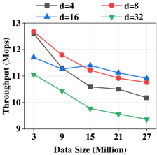
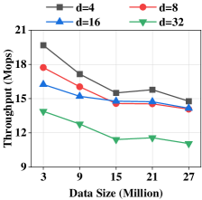
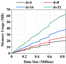


Effects of (Figure 2(a))-2(c): Our experimental results show that the optimal values of is 4 and 8. We find that and enable the fastest insertion and query throughput of CuckooGraph, respectively. Also, the memory usage of CuckooGraph with and is the least and second least, respectively. Considering that smaller means smaller , we set .
Effects of (Figure 3(a))-3(c): Our experimental results show that the overall performance is best when the value of is 0.9. We find that the insertion and query throughput of CuckooGraph with of 0.8, 0.85, and 0.9 are very close to each other, and all are faster than the one at of 0.95. In addition, the larger is, the smaller the memory usage of CuckooGraph is. Thus, we set after the above considerations.
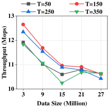
Effects of (Figure 4(a))-4(c): The experimental results show that CuckooGraph achieves most ideal performance at of 150 and 250. We find that CuckooGraph has the fastest insertion and query throughput when is 150 and 250, respectively. Meanwhile, different values of make no difference to the memory usage of CuckooGraph. Hence, we set .
V-C Experiments on Loading Rate
We conduct this loading rate experiment to verify that a single S-CHT can achieve a very high loading rate without insertion failure under our settings. For example, assuming that the first insertion failure occurs when the loading rate is 0.95, the probability of insertion failure when the loading rate is below 0.8 is extremely low (no Denylist is involved). Specifically, given the length of S-CHT, we use of the dataset to continuously insert S-CHT until the first insertion failure occurs, and output the loading rate of the S-CHT at this moment.

Results & Analysis (Figure 5): On different datasets and S-CHTs of different lengths, the loading rate can almost always reach above 0.95 (commonly to reach above 0.98) before the first insertion failure occurs. It shows that our S/L-CHT with two bucket array length ratio of 2:1 and can achieve extremely high loading rate, and the probability of insertion failure occurring below our setting of is extremely low.
V-D Experiments on Expansion Time
CuckooGraph’s S-CHT faces expansion during the insertion process, and only the Transformation from the 2n/n/n form to the 4n/2n form is the most time-consuming. The above time-consuming mainly lies in the operation of merging three 2n/n/n tables into one 4n table. Therefore, we use this experiment to explore how time-consuming such a merging operation is. Specifically, we use the deduplicated to continuously insert into these 3 empty tables so that their loading rate reach 0.8, then merge them and calculate the time spent on the merging operation.
Results & Analysis (Figure 6): The merging time has an approximately linear relationship with the S-CHT length. Although one merging may seem slightly longer, such time consumption is acceptable. Since the frequency of merging is very low, considering that merging only occurs once every many insertions, the AIT can still be stably maintained at a low value. Our Theorem 2 has shown that the AIT does not increase as the amount of data increases, but remains constant.
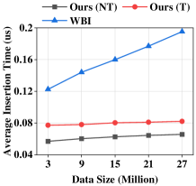
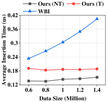
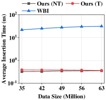
V-E Experiments on Edge Queries
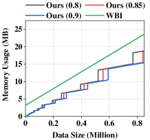
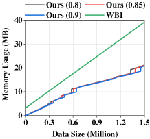
Methodology: 1) We insert a certain number of edges from the dataset into CuckooGraph or WBI and get the total insertion time, calculate it divided by the number of insertions to get the AIT. 2) We query the inserted edges sequentially and get the total query time and calculate it divided by the number of queries to get the AQT. 3) We first deduplicate the dataset with duplicate edges and obtain non-duplicated edges, and then insert them into CuckooGraph or WBI in sequence. After each insertion, the memory usage of CuckooGraph or WBI at that moment is output in sequence.
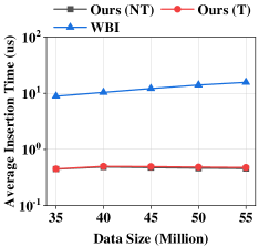
AIT (Figure 7(a)-7(d)): We find that the AIT of the NT and T states of CuckooGraph is around 24.0 and 21.6 lower than that of WBI on average, respectively.
AQT (Figure 8(a)-8(d)): We find that the AQT of the NT and T states of CuckooGraph is around 51.5 and 44.6 lower than that of WBI on average, respectively.
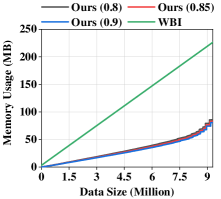
MU (Figure 9(a)-9(d)): We find that the MU of CuckooGraph at the three loading rates (0.8, 0.85, 0.9) is around 2.34, 2.46, and 2.56 lower than that of WBI on average, respectively.
Analysis: The time complexity of CuckooGraph insertion and query is without considering the time-consuming changes of the hash function modulo operations. The maximum number of L-CHT and S-CHT per cell is 3, and the lengths of L-DL and S-DL are also limited. Assuming that accessing a bucket or a Denylist requires one memory access, the worst case scenario when querying an edge is no more than 14 memory accesses, so there is an upper bound for the number of memory accesses in CuckooGraph. We can also demonstrate that the AIT in the worst case is no more than 3 times the above insertion time for a single insertion that does not involve Transformation. Conversely, since the adjacency matrix size of WBI is fixed, its insertion and query time increase as the number of different inserted edges increases, and the fixed adjacency matrix makes it poorly adaptable to graph scale changes. In terms of space usage, WBI suffers from several important drawbacks. First, WBI has to store a large number of pointers. CuckooGraph does not need to store a large number of additional pointers, and it has few structures that are not directly used for storage. Its space waste comes mainly from L/S-CHTs not being filled, but this is compensated for by the fact that its upper limit on the loading rate can be very high. Second, in WBI, assuming that a corresponds to , the has to be stored times in the linked list “blocks” corresponding to those different edges. When is large, such repeated storage imposes a large space overhead. Conversely, in CuckooGraph, unless has a corresponding that is kicked to S-DL, the need only be stored once and there is no duplicate storage. Third, WBI requires additional storage of additional data structures such as an adjacency matrix and counters. If the adjacency matrix is set too large in advance due to unpredictable data volume, it will cause huge waste of space. Conversely, CuckooGraph can flexibly handle any data volume.


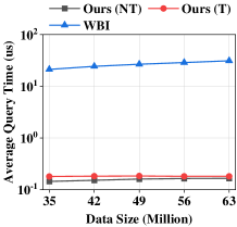
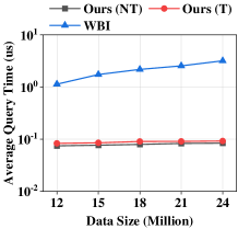

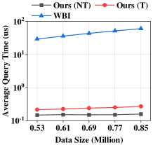
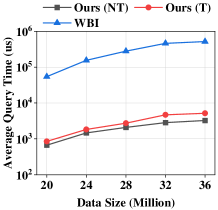
V-F Experiments on 1-Hop Successor and Precursor Queries
V-F1 1-Hop Successor Queries
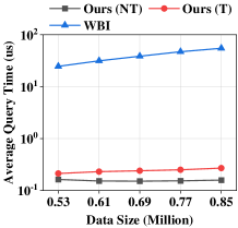
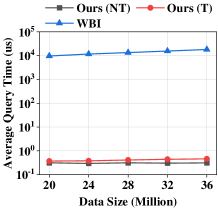
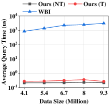
Methodology: This type of query refers to giving a and returning all its and their number. For CuckooGraph, it means finding the cell () or all S-CHT () corresponding to the , and returning all among them. In addition, S-DL must also be traversed and queried in case there is a corresponding to the . For WBI, we first find all the rows corresponding to the on the adjacency matrix, traverse all the edges hanging under these rows to find all the edges corresponding to the and return their corresponding . We evaluate this by inserting a certain number of non-duplicate edges, after which we randomly pick 5000 of the inserted for successor queries and calculate the AQT.
AQT (Figure 10(a)-10(d)): We find that the AQT of the NT and T states of CuckooGraph is around 13500.8 and 9994.7 lower than that of WBI on average, respectively.


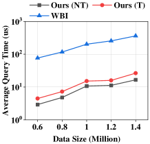


V-F2 1-Hop Precursor Queries
Methodology: This type of query is the opposite of the above-mentioned successor query, , given a , all its and their number are returned. Note that for , we need to insert it into CuckooGraph according to , , insert it in reverse. For WBI, we can insert normally like the above successor, but when querying the predecessor, we need to change “traverse all rows corresponding to ” to “traverse all columns corresponding to ”.
V-F3 Analysis
First, successor queries of WBI need to traverse a huge number of irrelevant other edges, resulting in a lot of waste of overhead. On the contrary, except that CuckooGraph may traverse a small number of edges of other in S-DL, the rest of the traversed are all based on the target . In short, the amount it traverses is much smaller than that of WBI. Second, the linked list “blocks” used by WBI to store edges are connected by pointers. Therefore, the addresses of different blocks may be far apart, and the spatial locality is very poor, so that traversing WBI may require a huge amount of memory accesses. As for CuckooGraph, basically exists in a small number of S-CHTs. Therefore, different can be arranged much more continuously in address with good spatial locality, which can greatly reduce the number of memory accesses. The analysis of the precursor queries is similar to that of the successor queries and will not be described in detail.
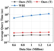
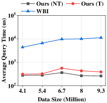
V-G Experiments on Finding Triangles
Methodology: Finding triangles means that given a node, return the number of triangles containing the node in the graph. For this query, WBI first finds all the precursors and all successors of the node, and then enumerates all possible edges composed of these successors and precursors to perform edge queries. The number of successful queries is the result of this task. CuckooGraph first finds all the 2-hop successors of the node through successor queries, and then enumerates all the possible edges composed of the node’s 2-hop successors and the node itself to perform edge queries. The evaluation method is also similar to Section V-F.
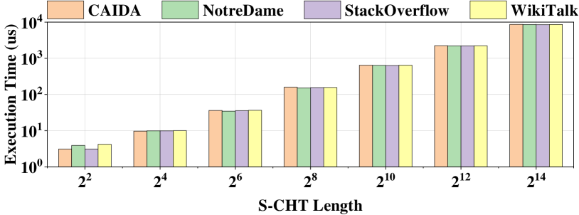
AQT (Figure 12(a)-12(d)): We find that the AQT of the NT and T states of CuckooGraph is around 136.5 and 75.2 lower than that of WBI on average, respectively.
Analysis: The reason is that CuckooGraph’s successor, precursor, and edge queries are all much faster than WBI’s. Because finding triangles is accomplished based on the successor, precursor and edge queries.
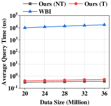
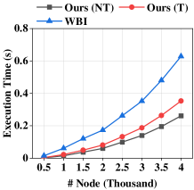
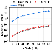
V-H Experiments on SSSP
Methodology: The details of the Single-Source Shortest Paths (SSSP) task are as follows. We first insert all the non-repeating edges of the dataset, and then select a number of nodes with the largest total degree (, the sum of the outgoing and incoming degrees) to extract the subgraph. After that, we take the 10 nodes with the largest total degree among these nodes, and execute Dijkstra algorithm [38] 10 times with these 10 nodes as the source. Each time Dijkstra algorithm is used to find the shortest distance from the source to the node on the subgraph for each node in the subgraph. We evaluate the execution time of these 10 tests. In Dijkstra algorithm, whenever an edge query is needed, an edge query of CuckooGraph or WBI is executed. Note that in this experiment, we default to a weight of 1 for all edges.
Execution Time (Figure 13(a)-13(d)): We find that the Execution Time of the NT and T states of CuckooGraph is around 132.8 and 103.7 lower than that of WBI on average, respectively.
Analysis: The reason why CuckooGraph is faster than WBI in this experiment is because CuckooGraph’s edge query is faster than WBI, especially when the amount of data is large.
V-I Other Evaluations
V-I1 From Real-World Graphs to Dense Graphs
The real-world datasets used in the experiments before this section are all sparse graphs. In order to verify that CuckooGraph is also effective on dense graphs, we synthesize the DenseGraph dataset and use AIT, AQT, and MU as the evaluation metrics.
V-I2 A Discussion with Graph Stream Summarization
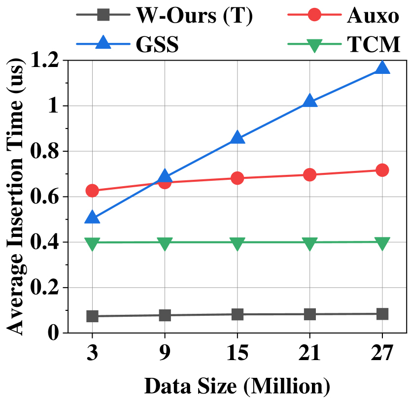
In recent years, the research community has proposed a series of graph stream summarization schemes [39, 40, 41, 42, 43, 44, 45] to approximately store graph streams in sublinear space, which is a different problem from the one concentrated in this paper. Next, we kindly compare and discuss three graph stream summarization schemes (Auxo [45], GSS [41], and TCM [40]) with the extended version of CuckooGraph (W-ours) on weighted edge queries in terms of AIT and AQT on CAIDA.
Results & Analysis (Figure 15(a)-15(b)): We find that both AIT and AQT of CuckooGraph are always faster than Auxo/GSS/TCM on weighted edge queries. However, these experiments are not comparisons between similar solutions, but are intended as friendly comparisons for discussion purposes only. It is clear that CuckooGraph/WBI records complete graph information, while Auxo/GSS/TCM approximately records graph streams, so they each have their own advantages and disadvantages and are designed for different scenarios and requirements.

VI Conclusion
This paper proposes CuckooGraph, a storage scheme that is error-free, efficient, and can flexibly adapt to large-scale dynamic graphs. CuckooGraph consists of two key techniques: Transformation and Denylist. Transformation allows flexible spatial transformation based on the arrival of items to maximize memory space utilization; Denylist efficiently accommodates failed insertion items and cooperates with Transformation to speed up item processing. Theoretical analysis of CuckooGraph is provided. We evaluate CuckooGraph on multiple important graph tasks on four large-scale real-world datasets and one synthetic dense graph dataset. Experimental results show that CuckooGraph significantly outperforms the SOTA scheme.
References
- [1] J. Li, X. Wang, K. Deng, X. Yang, T. Sellis, and J. X. Yu, “Most influential community search over large social networks,” in 2017 IEEE 33rd International Conference on Data Engineering (ICDE), 2017, pp. 871–882.
- [2] Y. Matsunobu, S. Dong, and H. Lee, “Myrocks: Lsm-tree database storage engine serving facebook’s social graph,” Proceedings of the VLDB Endowment, vol. 13, no. 12, pp. 3217–3230, 2020.
- [3] J. Zhang, C. Gao, D. Jin, and Y. Li, “Group-buying recommendation for social e-commerce,” in 2021 IEEE 37th International Conference on Data Engineering (ICDE), 2021, pp. 1536–1547.
- [4] D. Wang, J. Lin, P. Cui, Q. Jia, Z. Wang, Y. Fang, Q. Yu, J. Zhou, S. Yang, and Y. Qi, “A semi-supervised graph attentive network for financial fraud detection,” in 2019 IEEE International Conference on Data Mining (ICDM), 2019, pp. 598–607.
- [5] J. Jiang, Y. Li, B. He, B. Hooi, J. Chen, and J. K. Z. Kang, “Spade: a real-time fraud detection framework on evolving graphs,” Proceedings of the VLDB Endowment, vol. 16, no. 3, pp. 461–469, 2022.
- [6] X. Huang, Y. Yang, Y. Wang, C. Wang, Z. Zhang, J. Xu, L. Chen, and M. Vazirgiannis, “Dgraph: A large-scale financial dataset for graph anomaly detection,” Advances in Neural Information Processing Systems, vol. 35, pp. 22 765–22 777, 2022.
- [7] M. Iliofotou, P. Pappu, M. Faloutsos, M. Mitzenmacher, S. Singh, and G. Varghese, “Network monitoring using traffic dispersion graphs (tdgs),” in Proceedings of the 7th ACM SIGCOMM Conference on Internet Measurement, 2007, pp. 315–320.
- [8] T. Wang and L. Liu, “Privacy-aware mobile services over road networks,” Proceedings of the VLDB Endowment, vol. 2, no. 1, pp. 1042–1053, 2009.
- [9] M. Simeonovski, G. Pellegrino, C. Rossow, and M. Backes, “Who controls the internet? analyzing global threats using property graph traversals,” in Proceedings of the 26th International Conference on World Wide Web, 2017, pp. 647–656.
- [10] Y. Ma, P. Gerard, Y. Tian, Z. Guo, and N. V. Chawla, “Hierarchical spatio-temporal graph neural networks for pandemic forecasting,” in Proceedings of the 31st ACM International Conference on Information & Knowledge Management (CIKM), 2022, pp. 1481–1490.
- [11] X. Zhu, X. Huang, L. Sun, and J. Liu, “A novel graph indexing approach for uncovering potential covid-19 transmission clusters,” ACM Transactions on Knowledge Discovery from Data, vol. 17, no. 2, pp. 1–24, 2023.
- [12] J. Mondal and A. Deshpande, “Managing large dynamic graphs efficiently,” in Proceedings of the 2012 ACM SIGMOD International Conference on Management of Data, 2012, pp. 145–156.
- [13] P. Pandey, B. Wheatman, H. Xu, and A. Buluc, “Terrace: A hierarchical graph container for skewed dynamic graphs,” in Proceedings of the 2021 International Conference on Management of Data (SIGMOD), 2021, pp. 1372–1385.
- [14] J. Hou, Z. Zhao, Z. Wang, W. Lu, G. Jin, D. Wen, and X. Du, “Aeong: An efficient built-in temporal support in graph databases,” Proceedings of the VLDB Endowment, vol. 17, no. 6, pp. 1515–1527, 2024.
- [15] M. Potamias, F. Bonchi, A. Gionis, and G. Kollios, “K-nearest neighbors in uncertain graphs,” Proceedings of the VLDB Endowment, vol. 3, no. 1-2, pp. 997–1008, 2010.
- [16] U. Kang, H. Tong, J. Sun, C.-Y. Lin, and C. Faloutsos, “Gbase: an efficient analysis platform for large graphs,” The VLDB Journal, vol. 21, pp. 637–650, 2012.
- [17] S. Sahu, A. Mhedhbi, S. Salihoglu, J. Lin, and M. T. Özsu, “The ubiquity of large graphs and surprising challenges of graph processing,” Proceedings of the VLDB Endowment, vol. 11, no. 4, pp. 420–431, 2017.
- [18] Y. Shao, B. Cui, L. Chen, L. Ma, J. Yao, and N. Xu, “Parallel subgraph listing in a large-scale graph,” in Proceedings of the 2014 ACM SIGMOD international conference on Management of Data, 2014, pp. 625–636.
- [19] Y.-Y. Jo, M.-H. Jang, S.-W. Kim, and S. Park, “Realgraph: A graph engine leveraging the power-law distribution of real-world graphs,” in The World Wide Web Conference, 2019, pp. 807–817.
- [20] Z. Wei, X. He, X. Xiao, S. Wang, Y. Liu, X. Du, and J.-R. Wen, “Prsim: Sublinear time simrank computation on large power-law graphs,” in Proceedings of the 2019 International Conference on Management of Data (SIGMOD), 2019, pp. 1042–1059.
- [21] C. Wang, W. Wang, J. Pei, Y. Zhu, and B. Shi, “Scalable mining of large disk-based graph databases,” in Proceedings of the tenth ACM SIGKDD International Conference on Knowledge Discovery and Data Mining, 2004, pp. 316–325.
- [22] L. Zou, M. T. Özsu, L. Chen, X. Shen, R. Huang, and D. Zhao, “gstore: a graph-based sparql query engine,” The VLDB journal, vol. 23, pp. 565–590, 2014.
- [23] W. Sun, A. Fokoue, K. Srinivas, A. Kementsietsidis, G. Hu, and G. Xie, “Sqlgraph: An efficient relational-based property graph store,” in Proceedings of the 2015 ACM SIGMOD International Conference on Management of Data, 2015, pp. 1887–1901.
- [24] X. Zhu, G. Feng, M. Serafini, X. Ma, J. Yu, L. Xie, A. Aboulnaga, and W. Chen, “Livegraph: a transactional graph storage system with purely sequential adjacency list scans,” Proceedings of the VLDB Endowment, vol. 13, no. 7, pp. 1020–1034, 2020.
- [25] A. Mhedhbi, P. Gupta, S. Khaliq, and S. Salihoglu, “A+ indexes: Tunable and space-efficient adjacency lists in graph database management systems,” in 2021 IEEE 37th International Conference on Data Engineering (ICDE), 2021, pp. 1464–1475.
- [26] “Neo4j website.” https://neo4j.com/, 2022.
- [27] “OrientDB website.” http://orientdb.org/, 2020.
- [28] “ArangoDB website.” https://www.arangodb.com/, 2021.
- [29] “JanusGraph website.” https://janusgraph.org/, 2021.
- [30] “GraphDB website.” https://www.ontotext.com/products/graphdb/, 2022.
- [31] R. Qiu, Y. Ming, Y. Hong, H. Li, and T. Yang, “Wind-bell index: Towards ultra-fast edge query for graph databases,” in 2023 IEEE 39th International Conference on Data Engineering (ICDE), 2023, pp. 2090–2098.
- [32] R. Pagh and F. F. Rodler, “Cuckoo hashing,” Journal of Algorithms, vol. 51, no. 2, pp. 122–144, 2004.
- [33] “Hash website,” http://burtleburtle.net/bob/hash/evahash.html.
- [34] “The CAIDA Anonymized Internet Traces,” https://www.caida.org/catalog/datasets/overview/.
- [35] “Note Dame web graph,” http://snap.stanford.edu/data/web-NotreDame.html.
- [36] “Stack Overflow temporal network,” http://snap.stanford.edu/data/sx-stackoverflow.html.
- [37] “Wikipedia talk (en),” http://konect.cc/networks/wiki_talk_en/.
- [38] E. W. Dijkstra, “A note on two problems in connexion with graphs,” in Edsger Wybe Dijkstra: His Life, Work, and Legacy, 2022, pp. 287–290.
- [39] P. Zhao, C. C. Aggarwal, and M. Wang, “gsketch: on query estimation in graph streams,” Proceedings of the VLDB Endowment, vol. 5, no. 3, pp. 193–204, 2011.
- [40] N. Tang, Q. Chen, and P. Mitra, “Graph stream summarization: From big bang to big crunch,” in Proceedings of the 2016 International Conference on Management of Data (SIGMOD), 2016, pp. 1481–1496.
- [41] Gou, Xiangyang and Zou, Lei and Zhao, Chenxingyu and Yang, Tong, “Fast and accurate graph stream summarization,” in 2019 IEEE 35th International Conference on Data Engineering (ICDE), 2019, pp. 1118–1129.
- [42] X. Gou, L. Zou, C. Zhao, and T. Yang, “Graph stream sketch: Summarizing graph streams with high speed and accuracy,” IEEE Transactions on Knowledge and Data Engineering, vol. 35, no. 6, pp. 5901–5914, 2023.
- [43] J. Ko, Y. Kook, and K. Shin, “Incremental lossless graph summarization,” in Proceedings of the 26th ACM SIGKDD International Conference on Knowledge Discovery & Data Mining, 2020, pp. 317–327.
- [44] Z. Ma, J. Yang, K. Li, Y. Liu, X. Zhou, and Y. Hu, “A parameter-free approach for lossless streaming graph summarization,” in Proceedings of the 26th International Conference Database Systems for Advanced Applications (DASFAA), 2021, pp. 385–393.
- [45] Z. Jiang, H. Chen, and H. Jin, “Auxo: A scalable and efficient graph stream summarization structure,” Proceedings of the VLDB Endowment, vol. 16, no. 6, pp. 1386–1398, 2023.