Addressing Duplicated Data in Point Process Models
Abstract
Spatial point process models are widely applied to point pattern data from various fields in the social and environmental sciences. However, a serious hurdle in fitting point process models is the presence of duplicated points, wherein multiple observations share identical spatial coordinates. This often occurs because of decisions made in the geo-coding process, such as assigning representative locations (e.g., aggregate-level centroids) to observations when data producers lack exact location information. Because spatial point process models like the Log-Gaussian Cox Process (LGCP) assume unique locations, researchers often employ ad hoc solutions (e.g., jittering) to address duplicated data before analysis. As an alternative, this study proposes a Modified Minimum Contrast (MMC) method that adapts the inference procedure to account for the effect of duplicates without needing to alter the data. The proposed MMC method is applied to LGCP models, with simulation results demonstrating the gains of our method relative to existing approaches in terms of parameter estimation. Interestingly, simulation results also show the effect of the geo-coding process on parameter estimates, which can be utilized in the implementation of the MMC method. The MMC approach is then used to infer the spatial clustering characteristics of conflict events in Afghanistan (2008-2009).
Keywords: Conflict events; Duplicates; Geolocation error; LGCP; Spatial point process
1 Introduction
Event data (i.e., presence-only data) are commonly found in various fields, such as environmental sciences, population ecology, sociology, and political science. In the social sciences, for example, they are used to analyze spatial patterns of social and political behavior, including analyses of protests (Earl et al., 2004), crime (Krieger et al., 2015), terrorism (LaFree, 2019), and civil violence (Cederman and Gleditsch, 2009). These data code actions at the incident level – that is, they provide who-did-what-when-where-and-why information on discrete events – thereby allowing for greater insights into their determinants. Given continued improvements in our ability to automate event identification and extraction from secondary sources (Lee et al., 2019), event data are likely to see even wider use in the future.
Much of the promise of event data analysis in social science applications, however, is often unrealized due to the well-known limitations of these data (e.g., missing events, geolocation errors, etc.). Event data in social sciences are largely drawn from media reports, which risks description bias as event details may go inaccurately reported (Earl et al., 2004). This can include information as basic as where the event occurred (Weidmann, 2015). Oftentimes, for example, the initial media report may contain imprecise information on the event location, providing only the district or state within which it occurred (Cook and Weidmann, 2022). In these instances, researchers often assign representative spatial coordinates (i.e., the observations are snapped), such as the centroid for the administrative unit in which the event was reported.
While this may be the best that can be achieved, given the inherent limits on the available information, these geo-coding decisions present problems for analysts interested in applying point process models. First, the assigned locations may deviate considerably from the true locations, i.e., geolocation error, threatening the validity of any inferences drawn using the observed point pattern. Second, the likelihood of duplicated data rises dramatically since multiple events may be assigned to the same location. Duplicated data creates issues when applying spatial point process models, as these often assume non-coincident observations. For instance, under the spatial Log-Gaussian Cox Process (LGCP) framework, having more than one event at the same location results in a non-invertible covariance matrix for the underlying Gaussian process. Therefore, in order to apply spatial (and spatio-temporal) point process models, researchers are forced to address the issue of duplicated data.
Various approaches have been implemented in the literature to address these duplicates, including data elimination (i.e., dropping duplicate observations) and data manipulation (i.e., jittering event locations). While these may evade the issue of duplicate points, this is achieved at a great cost, as these strategies induce sample selection bias and errors in location information. Given these costs, we propose a more principled approach to accommodate data with duplicates during estimation: the modified minimum contrast (MMC) method. The key insight advanced here is that with minimal changes to the information supplied to the objective function – through the introduction of a non-zero lower bound to the lag limit used in the discrepancy measure – we can avoid the adverse effect of duplicate events on inference. This approach not only solves problems with duplicate observations but may also improve inference with data exhibiting more general geolocation errors.
The rest of the paper is organized as follows. Section 2 introduces the causes and consequences of duplicated points and summarizes existing methods to address duplicates. We then provide two motivating real-world examples to demonstrate how duplicates arise and their effect on Ripley’s -function, a widely used summary statistic for point processes. In Section 3, we define and introduce the relevant properties of LGCP models before proposing the MMC estimation method for inference adjustment when analyzing observed point patterns containing duplicates. Then, in Section 4, we design three simulation scenarios to illustrate the performance of the proposed method as compared to existing methods. Finally, in Section 5, we apply these same approaches to real-world conflict data from Afghanistan before concluding in Section 6.
2 Motivation
In incident-level data, there are two types of duplicated data that researchers often confront: i) multiple entries for the same incident and ii) multiple incidents with the same spatial coordinates. In the former, multiple records of the same event are entered into the sample – arising from multiple reports, etc. – and should be removed in the data processing stage (i.e., de-duplication) prior to analysis. In the latter, duplicate data (or duplicated points) arise when separate events or incidents are assigned the same spatial coordinates. As these are independent events, they should each remain in the sample; however, the coincident location information can pose challenges in subsequent spatial point pattern analysis. This is the issue we concentrate on here.
Duplicated points can arise in many ways; however, they typically occur because of imprecision in the measuring instrument, coding choices made in data processing, or both. At sufficiently high levels of resolution, the probability of multiple events occurring in the same location should approach zero. Our measures of these incident locations, however, are rarely this precise, meaning the recorded locations nearby can and often do coincide. Still other times, duplicate data are produced due to deliberate decisions made in data publishing. When there are (geo)privacy concerns relating to the data, for example, incident locations may be “snapped” to the nearest notable spatial feature, thereby risking duplicate points. See Figure 1 for what we mean by “snapping.” In the Police.uk data (Tompson et al., 2015), for example, the actual crime event location is obfuscated by snapping to the nearest point from a predetermined list of connotatively neutral locations to protect confidentiality. This process – one of the geographic masking techniques presented in Zandbergen (2014) – likely inflates the number of duplicate points we observe because each snap point may have multiple events near it, resulting in those crimes being assigned to the same geographic coordinates.
In other instances, duplicates can arise due to both data imprecision and resultant coding decisions, as in many social and political events datasets. To illustrate, consider the Global Terrorism Database (GTD; START, 2021a), which draws from publicly available information, e.g., media reports, to produce data on incidents of domestic and international terrorism. These media reports often lack precise information on the location of the incident, indicating only a general area in which the event took place. Lacking exact location information, the spatial coordinates of the event are instead assigned/snapped to the centroid of the smallest administrative region identified. These coding conventions are commonly found in media-sourced event data and inevitably incur duplicate points. In what follows, we refer to point patterns with snapping-induced duplicates as corrupted data.
Regardless of their origin, duplicate points pose several challenges when applying statistical methodology to spatial point processes. Many point process models are based on the assumption that the underlying true processes are simple, i.e., no two points coincide in the same position (Daley and Vere-Jones, 2003, p.47). Duplicated points violate this assumption, and statistical procedures designed for simple point processes will be invalid or non-applicable (Baddeley et al., 2015, p.60). For example, in parameter estimation procedures of LGCP models that involve covariance matrices, such as maximum likelihood estimation, duplicated points lead to non-invertible covariance matrices or ill-conditioned optimization problems. For LGCP models, even for inference methods that do not deal with covariance matrices, such as minimum contrast estimation, the presence of duplicates may produce biased estimates of parameters that characterize the underlying spatial point process. Specifically, duplicated points artificially inflate the observed count of points within small distance lags (as later seen in Figure 3). Duplicated points may form clusters that do not reflect genuine spatial clustering but instead arise from the duplication itself, leading to biased estimates of parameters associated with spatial clustering in the model. As such, researchers need to carefully consider the issue of duplicates in spatial point process modeling.
Handling of Duplicates
There is no single, easy approach to address duplicate data fully. Obviously, ignoring the presence of duplicates and blindly applying inference methods is inadvisable as one would obtain unreliable and misleading results. However, we will later use this “do nothing” approach as a baseline for comparison. In our review of the relevant literature on spatial point pattern data, we found several more direct approaches to dealing with duplicates used in applied research.
First, researchers can simply remove duplicated points from the data (Method \Romannum1). By deleting all but one observation at each location where duplication occurs (Turner, 2009), researchers ensure there is no duplicate data in the analysis sample. However, this is achieved at some cost since removing these duplicates results in a loss of information from the data and biased inferences, especially the underestimation of first-order intensity.
Second, researchers may jitter the locations of duplicated points (Method \Romannum2). Here, one adds a random perturbation to the coordinates of each duplicated point (e.g., Iftimi et al., 2018; Jun and Cook, 2024), which again effectively eliminates duplicate points. For instance, one may jitter the - and -coordinates of the duplicated point independently by amounts chosen from a uniform distribution for some . Unlike deletion, this method allows researchers to retain all of the data; however, it is sensitive to ad hoc choices regarding the jittering distribution(s). There is no established method to guide these choices, and it can be challenging to determine the optimal jittering radius, , that effectively removes the artifacts caused by duplicated points without overly damaging the integrity of the original spatial pattern. For example, one may set a small number for to alleviate the problem of the point process not being simple without altering the data too much, but the effect of duplicates (i.e., microspatial aggregation) may not be adequately addressed. For example, if the duplicates are created due to corruption, as seen in the GTD mentioned above, the optimal jittering radius, though unknown, is clearly not small because the maximum error introduced through snapping points to centroids grows with the size of the domain partitions. On the other hand, if is too large, it may excessively disrupt the spatial structure of the data, and one even runs the risk of pushing points (near the boundary) out of the study domain. Regardless of the specific choices made, ultimately, one induces spatial measurement error in the original sample, which necessarily carries some costs.
Lastly, as with jittering, researchers may redistribute duplicated points to other randomly determined locations within some predetermined area (Method \Romannum3). For example, one may replace each duplicated point with a random point within some associated partition area, e.g., a Thiessen polygon or a geographical unit that contains the original point. While this is more often applied for disaggregating count data as in Shi et al. (2013), it can also be applied to address duplicates. Unlike jittering in Method \Romannum2, this method ensures that points near the boundary of the study domain are retained. However, it still introduces additional noise to the data, the extent of which is subject to the size and shape of the partition areas. As a result, the induced error will be larger on average for events in large partitions than for events in small ones. Additionally if event determinants (e.g., population) are also correlated with the size of these units, then the induced noise can produce a form of differential measurement error.
Case Study – Afghanistan
We first consider the GTD data on terrorism to demonstrate the extent and severity of these issues in real-world data. In the GTD, incidents of terrorism are collected primarily from publicly available, unclassified source materials, e.g., media articles and electronic news archives (START, 2021b). Most GTD events are assigned precise latitude and longitude data, and the presumed level of accuracy in these locations is reported as an additional feature in the data set. This accuracy is encoded by a “specificity” score, an ordinal measure ranging from 1 (very accurate) to 5 (location unknown). For example, specificity indicates the spatial coordinates of the event are assigned at the most specific spatial resolution – the center of the city, village, or town in which the attack occurred; specificity indicates the coordinates of the event are less accurate and assigned at the centroid of the smallest subnational administrative region identified, e.g., subdistrict, district, province, etc.; specificity means the longitude and latitude of the event are unknown (additional details are given in START (2021b)).


Figure 2 shows the prevalence of duplicates in the GTD data on Afghanistan between 2011 and 2020. We observe that more than half of the events have a specificity level greater than 1 (in (a)), and more than of points in any given year are duplicated (in (b)). This indicates that spatial uncertainty and duplication persist in this data set over time. Additionally, among events with specificity = 1, the highest level of precision, the duplication (multiplicity ) is still present, as shown in (c). This may be partially due to urban/populated areas being more likely to be the targets of terror attacks, and the highest spatial resolution in the data set is the center of the city in which attacks took place.
While self-reported information on the locational uncertainty is useful, contrasting media-sourced data with more accurate (ideally gold-standard) data would obviously be preferred. With this in mind, we next consider a data set used in Weidmann (2015), which has drawn from two sources reporting conflict events in Afghanistan: i) the “Significant Activities” (SIGACTS) military database, and ii) the UCDP Geo-referenced Event Dataset (GED; Sundberg and Melander, 2013). For matched pairs, i.e., events appearing in both data sets, we have two reported locations – one from the GED and one from SIGACTS – for each observation. Like the GTD data, the GED data are drawn from media reports and contain many duplicates. On the other hand, locations in SIGACTS are measured with GPS technology; hence, they are more accurate and contain far fewer duplicates. The availability of conflict event data compiled independently by both the media (GED) and the military (SIGACTS) makes these data sets one of the few opportunities for a data set comparison.
To illustrate the effect of corrupted data on summary statistics, we compare the estimated Ripley’s -function (Ripley, 1977) from the GED to that from the SIGACTS data. The stationary homogeneous -function is defined as where is the (assumed) constant intensity, and is the random number of extra points within distance of an arbitrary point of the process. The function is typically estimated by given later in equation (6). The distance metric we use here is Euclidean distance on planar coordinates. One could work with geodesic distance using longitude and latitude, but given the relatively small spatial domain we consider, we decided to use a projection instead. Specifically, we convert geographic (latitude, longitude) coordinates from GTD to the Universal Transverse Mercator (UTM) coordinates (where unit distance is km).

Figure 3 shows estimated functions for the SIGACTS data, the original GED data, and the GED data with the three methods to handle duplicates described above. We see that the for the unmodified GED presents a discontinuity near the origin, caused by duplicates; moreover, after (km), it consistently underestimates compared to the for SIGACTS. Though the discontinuity disappears after a small amount of jittering ( km) for each coordinate using MC-\Romannum2, the corresponding looks essentially similar to the unmodified data. A large ( km) jittering radius behaves similarly to MC-\Romannum3, as they both spread duplicated points to such a degree that they severely underestimate . Worse still is the from MC-\Romannum1, which produces the lowest estimated values given the deleted observations. Note that the ’s corresponding to each of these methods to deal with duplicates show a certain level of deviation from the reference for SIGACTS, which may lead to poor performance in parameter estimation using -function-based statistical inference (e.g., minimum contrast estimation with -function).
3 Modified Inference for Point Patterns with Duplicates
Each of the methods to deal with duplicates introduced above modify the original spatial point pattern data in some manner, either by deleting, jittering, or redistributing observations. To develop a more principled method for handling duplicates, we refrain from altering data and instead develop an inference method to accommodate duplicated data. Our proposed method works with the original, unaltered data, even when duplicates are present. Furthermore, as illustrated below through simulation studies, our proposed method helps to uncover the nature of spatial corruption of the data. We focus here on duplicate data in the context of the LGCP, a widely used model for analyzing spatial point pattern data. In the following, we first introduce some necessary preliminaries on the LGCP framework and then detail our proposed duplicate-robust inference method, the Modified Minimum Contrast method.
Log-Gaussian Cox Process
Many point patterns from real-world data exhibit complex interactions between points, necessitating more flexible point process models. LGCPs (Møller et al., 1998) are well-developed and popular models for capturing spatial (and spatio-temporal) interactions among points in environmental studies (Valente and Laurini, 2023), ecology (Renner et al., 2015), and spatial epidemiology (Diggle et al., 2013). Political events typically present high heterogeneity and geographic clustering (Buhaug and Gleditsch, 2008; Darmofal, 2009), making LGCP models useful for elucidating such patterns.
An LGCP model can be specified in the following way: first level, the process is a Poisson process conditional on the intensity function ; second level, this intensity function is considered as a realization of the stochastic process , which is often expressed as in analogy with random effect models
| (1) |
where , is a vector of covariates at location , and are the associated parameters to be estimated; is a Gaussian random field. One appealing feature of the LGCP is that its moment properties are analytically tractable. In particular, the first-order characteristic intensity function is given by
| (2) |
where , and . The second-order characteristic pair correlation function (PCF) is given by
| (3) |
where is the correlation function of . For more theoretical properties of LGCPs, see Møller et al. (1998).
Throughout the remainder of the paper, we assume that is stationary and isotropic, implying that , and . We consider an exponential correlation function controlled by a parameter for such that . Moreover, we let for identifiability. The intensity and PCF in (2)-(3) are then simplified as
| (4) |
Under our assumptions and settings, spatial clusters captured by LGCPs are related to the spatial range parameter and the variance parameter . As either of these parameters tends to zero, so too does , meaning there is no spatial clustering. As in Zhu et al. (2021), note that increasing while holding fixed determines the sizes or radii of the clusters. If one instead holds fixed, then increasing determines the variance in the intensity across the spatial domain. Jointly increasing both and directly affects the dependence of process , producing larger clusters of points (due mainly to ) that are increasingly distinct from those points not in a given cluster (due mainly to ).
Three common statistical inference methods for LGCP models are maximum likelihood inference, Bayesian inference, and Minimum Contrast (MC) estimation. However, both maximum likelihood inference and Bayesian inference face challenges when applied to complex point processes like LGCPs due to analytically intractable likelihood functions, as discussed in Baddeley et al. (2007) and Møller and Waagepetersen (2017). Moreover, these methods may encounter numerical issues; in particular, the covariance matrices are non-invertible when the observed point pattern contains duplicates. On the other hand, the MC method (Møller et al., 1998; Diggle, 2003) is widely favored in practice owing to its computational efficiency and ease of implementation. Notably, MC methods can be directly applied to point patterns containing duplicates without numerical issues arising, though they do not account for the bias induced by the presence of duplicates. Hence, this study endeavors to adapt the MC method to accommodate the impact of duplicates within the LGCP framework.
Proposed Method: Modified Minimum Contrast
The main idea of the MC method is to look for parameters that minimize the discrepancy measure between the theoretical summary descriptor that involves the unknown parameters, and its empirical counterpart. In this study, we consider the -function as the summary descriptor to characterize the second-order properties of a point process.
Let denote the theoretical -function and the corresponding empirical estimate. A typical measure of discrepancy between and is
| (5) |
where and are given constants and is a weight function. The MC estimate for is then defined as the minimizer of . The asymptotic properties of the MC method can be found in Heinrich (1992) and in Guan and Sherman (2007).
For a stationary point process , is given by
| (6) |
where is the number of observed points inside a bounded window , is the index set of the events in , is an edge correction factor, and is the estimated intensity just as computed by the R package spatstat (Baddeley et al., 2015). We can see that when duplicates are present in data, overestimates when is small. In other words, the expected number of extra points within a relatively short distance of a randomly chosen point is overestimated, i.e., as we observed in Figure 3. Then, since we know that there will be an erroneous discrepancy between and at small values of , it is natural to truncate the integral to reflect only the true discrepancies. Hence, we modify the discrepancy measure in equation (5) by adding a tuning parameter as the lower limit of the integral, that is
| (7) |
The resulting minimizer we call the modified minimum contrast (MMC) estimator. We note that there are some literature that presents the general MC idea with the general lower bound of the integral in (5). However, as far as we are aware, this is the first thorough study to check the effect of non-zero lower bound in the discrepancy measure, and furthermore, the first study that demonstrates the utility of such non-zero lower bound in dealing with duplicates in spatial point pattern data.
As in the general MC methods, there are no standard criteria for choosing appropriate user-specified parameters , , and the weight function . For the weight function and the tuning parameter in equation (7), per Diggle’s suggestion (Diggle, 2003, p. 87) we let and . For , the upper limits of the discrepancy measure, Diggle suggests that a good rule of thumb is to set where and represent the maximum width and height of the study domain. However, in the case of heterogeneous point patterns, to capture the local features, a smaller should be used as in Davies and Hazelton (2013). Lastly, for the key tuning parameter , our hypothesis is that the optimal is associated with the geometry of the partitions for the study region, say the length of the cell on a regular grid. This will be discussed in greater detail in Section 4.
For a second-order intensity-reweighted stationary (SOIRS) point process, i.e., PCF is translation invariant if it exists, we then replace with , the estimate of the inhomogeneous -function proposed by Baddeley et al. (2000)
| (8) |
where is an estimate of the intensity function often by kernel smoothing approaches, which will be introduced in the next section. As for the theoretical (or parametric) -function, its mathematical form is known for many point processes. In particular, if is an LGCP under our setting in Section 3.1, the parametric -function is given by
| (9) |
Then the MMC estimate for is chosen to minimize
| (10) |
Replace by if is inhomogeneous.
First-Order Intensity Estimation
As in the MC method, the MMC method requires estimates of the first-order intensity function and the -function. We estimate the first-order intensity nonparametrically in all cases even when we know the true parametric settings (as in the simulated studies) because in real applications, not only do we not know the true heterogeneous trend, but even if one believes that some factors contribute to this heterogeneity, the relevant covariates are not always available to us. For an inhomogeneous point process with a smoothly spatially varying intensity, we consider a fixed-bandwidth kernel estimate for as proposed in Davies et al. (2018): for observed points ,
| (11) | ||||
where is the bandwidth, is the kernel function and is an edge-correction factor.
On the other hand, for an inhomogeneous point process with a moderately to highly heterogeneous intensity, we use an adaptive kernel estimator as in Davies and Baddeley (2018) and Davies et al. (2018). The idea of this approach is to allow the bandwidth to vary with respect to observations so that, in areas of high density, the resulting bandwidth is small, while in areas of low density, the resulting bandwidth is large. Formally, the adaptive estimator is given as
| (12) | ||||
where the smoothing bandwidth is a function of a coordinate, is a pilot estimate of the unknown intensity constructed via (11) with a fixed pilot bandwidth , is the global bandwidth, is the geometric mean of the inverse-density bandwidth factors, and is the edge correction for the adaptive estimator. For simplicity, we let . For details, see (Abramson, 1982; Silverman, 1986; Davies et al., 2018).
4 Simulation Study
We undertake a series of simulation experiments under different settings of the spatial structure of the point patterns as well as their corruption process and present key findings in this section. Additional results are presented in the Appendix.
Three main scenarios are considered as summarized in Table 1: , a homogeneous LGCP; , an inhomogeneous LGCP with a smooth spatially varying intensity structure; and , an inhomogeneous LGCP with a moderately heterogeneous intensity structure that resembles the real-world application. To facilitate comparison between these scenarios and to make these scenarios comparable to our main application, we use a square as the domain in and . This has an area roughly equal to that of Afghanistan itself (approx. 652,861 km2), which is used as the domain in . The expected number of points, , over the entire spatial domain for all three scenarios is set to be approximately 1,000, roughly the number of events in the paired SIGACTS/GED datasets.
Type of LGCP Label Domain Homogeneous Inhomogeneous Afghanistan
-
•
(, ) is the location vector, with and the x and y coordinates respectively.
-
•
log_cities represents the log of distance to the top 10 most populated cities in Afghanistan.
-
•
log_ring represents the log of distance to the ring road in Afghanistan.
-
•
The unit of distance for is km.
As discussed in Section 3.1, we assume that the second-order properties are controlled by an exponential correlation structure from the underlying Gaussian process such that and . Here denotes the Euclidean norm. For , we set and to produce mild and moderate spatial clustering. For scenarios S2 and S3, we only consider since, as discussed in Davies and Hazelton (2013), with larger , spatial clustering of points may be hard to separate from the spatially varying mean term, .
As observed in Figure 2, in the GTD terrorism data, approximately of points are duplicated in any given year. To parallel this, we corrupt the simulated data for all three scenarios by snapping of points to the centroid of their domain partitions so that roughly of the points are duplicated. When applying the proposed MMC method, we consider values ranging from and , considering the size of the domain. We repeat the simulations 200 times for each scenario and present the estimates of parameters against for both uncorrupted and corrupted synthetic data. We report the median of the estimates along with the first and third quartiles (Q1, Q3).
Homogeneous Case: S1
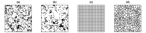
We start with the homogeneous LGCP, , where the expected number of points is 1,000 across the spatial domain. Figures 4(a)-(b) show realizations under with mild spatial clustering and moderate spatial clustering , respectively. To observe the effect that the shape and size of the partitions have on the results, we consider two types of domain partitions (e.g., pseudo-administrative divisions): a regular grid shown in Figure 4(c) and a Dirichlet tessellation shown in Figure 4(d). To form the corrupted data, we randomly select of the uncorrupted data in Figures 4(a) and (b) to be snapped to the centroid of each domain partition.
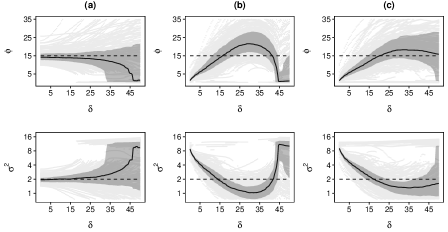
Figures 5 and 6 present the behavior of MMC estimates for parameters and against . Notice that, in both figures, when there is no data corruption (in (a)), the estimates of are nearly constant. This may be a sign that when there are no duplicates, the estimates of are not overly sensitive to the particular choice of , at least up to a certain point. On the other hand, we observe that both figures exhibit concavity between and for both types of corrupted data. For both Figures,(b) and (c) show that for corrupted data, the median of estimated values with (i.e., usual MC method) is much smaller than the true value. It is promising that, as increases from zero, the median of estimated values increases to reach near the true value. Moreover, the best median value is attained near the curve’s maximum, and the particular values that give the best estimates are around 25, which is about the maximum snapping distance for the simulation. This provides us guidance on choosing the optimal value (i.e., value that results in the best estimate).
On the other hand, the curve for in Figure 6 (b) has multiple local peaks (after the first largest one) that may correspond to the spatial design of grids for snapping. That is, the smallest snapping distance is around 25 (corresponding to the first peak), then around 50 (for the second peak), etc. This pattern is clearly an artifact of the geometry of the regular grid. This agrees with the fact that we no longer observe these sharp edges when tessellations are used to partition the domain (Figure 6 (c)). We want to point out that the optimal value is dependent upon the process of the data corruption (i.e., the shape and size of administrative districts) rather than the underlying second-order properties of the point patterns.
Regarding the selection of for parameter estimates, we suggest choosing the corresponding to the first local maximum in the median curve for corrupted data (which gives the largest estimate as discussed above). To be clear, we are not choosing that gives the closest estimate of to the true value, as this would be unknown in applied settings. Instead, we choose the that gives the maximum value, under the reasoning that duplicate data generally result in the underestimation of . This strategy can be applied to real data applications, and our simulation studies suggest that the maximum value of (under different candidate values for ) also tends to be closest to the true value.

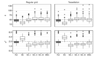
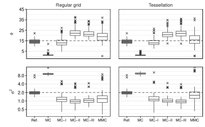
We now compare the performance, in terms of parameter estimation, of the proposed method with the MC method combined with existing methods to deal with duplicates. Figure 7 reports the estimates of and for various methods to deal with duplicates for the scenario . Here, “Ref” refers to the MC estimates when there is no corruption, “MC” refers to the MC estimates with duplicates, “MC-I” refers to the MC estimates with duplicates removed, “MC-II” refers to the MC estimates with jittering, “MC-III” refers to the MC estimates with re-distribution, and “MMC” refers to the proposed MMC method. Overall, it is clear that “MC” gives a serious underestimation of as expected. The rest of the MC methods are somewhat comparable, except that MC-I gives a reasonable estimate of . However, as discussed later in this section, MC-I has the problem of serious underestimation of the first-order intensity structure due to the fact that duplicates are simply removed. The problem will be more detrimental when there are significant amounts of duplicated points. Compared to MC-\Romannum2 and MC-\Romannum3, the proposed MMC method gives better estimates for in the sense that the median of the estimates is closer to the truth (despite a slightly larger variance).
Although MC-\Romannum2 may seem appealing at first, it requires a nontrivial choice to be made regarding the jittering radius. As discussed in Section 2, there is no standard approach to guide this choice. Figure 8 shows the effect of jittering radius in the estimates of and . As we can see, the estimated () is monotonically increasing (decreasing) with respect to the jittering radius. Furthermore, there is no clear reason why a jittering distance of km gives the best estimate of . Therefore, there is no way of identifying the optimal jittering distance that is likely to return the best estimates of in either simulation studies or real data applications. In contrast, as discussed above, we can identify optimal even for real data applications, as we choose that gives the maximum estimate. In our simulation studies, we chose to use a jittering radius of km, considering the size of the districts, as discussed above.

Inhomogeneous Case: S2
We next consider an inhomogeneous case, with a smoothly varying intensity surface (a linear function of coordinate components). As in , we corrupt the simulated data by moving of the points to the centroid of their pseudo-administrative divisions: a regular grid and a tessellation. Figure 9 shows a single realization and two corresponding corrupted point patterns to illustrate the difference between the corruption by the regular grid and by the tessellation.

The first-order intensity functions are estimated by kernel smoothing with fixed bandwidth, as illustrated in Section 3.3. We adopt the criteria by Davies and Hazelton (2013) with a modification to choose the bandwidth (over a sequence of values) that performs better in recovering the true values of parameters for uncorrupted data. More specifically, we define the Relative Euclidean Distance (RED) as
where and are absolute relative errors of MC estimates ( and ) from uncorrupted data. Next, instead of computing the mean of estimated parameters and then RED as in Davies and Hazelton (2013), we compute RED for estimated parameters and then take the median as the median provides a more stable measure of central tendency. By computing RED for each individual simulation, we gain the added benefit of computing error bounds for the bandwidth curves. We then pick the bandwidth that minimizes this median. In this simulation scenario, we get as the optimal bandwidth and use it for both the uncorrupted and corrupted data.

Figure 10 presents the MMC results for this scenario. We observe that the median of the estimates of against from the simulated data in (a) decreases with respect to and stays roughly constant () otherwise. In contrast, the median of estimated from both grid and tessellation corrupted data, (b)-(c), each show a local maximum at (similar to the optimal value chosen for S1). Figure 11 presents the results for and from the different approaches, similar to the comparison done for presented earlier in Figure 7. The results are similar to those from : MMC returns estimates closer to the truth than either MC-\Romannum2 or MC-\Romannum3, and as good if not better than MC-\Romannum1 (depending on the scenario). While method MC-\Romannum1, simply deleting duplicates, seems to capture second-order properties fairly well, this comes at the expense of accurately capturing the first-order intensity. As shown in Figure 12, deleting the duplicate data causes the model to heavily underestimate the first-order intensity structure. While not the central focus of our study, this has obvious consequences in applied research where the first-order intensity, often expressed as a function of spatial covariates, is central.


Inhomogeneous Case: S3
The final simulation scenario we consider is designed to parallel features of the paired SIGACTS/GED dataset, offering a more realistic setting to evaluate our approach. We implement the simulation within the boundary of Afghanistan and use its (second-level) administrative divisions (Figure 13(d)), 328 districts (obtained from the GADM database), as the domain partitions. Using this more realistic simulation setting also allows us to demonstrate how to select tuning parameters (e.g., bandwidth) necessary for analyzing real data.
As detailed in Table 1, we design a first-order intensity function as a linear combination of two covariates to generate point patterns with moderate-to-high heterogeneity. Specifically, this function has a strong negative association with the log of distance to the ring road (World Bank Group, 2019) and a relatively weaker negative association with the log of distance to the top ten most populated cities in Afghanistan (GeoNames, 2023); coefficients are adjusted so that the expected number of generated points is approximate 1000. In other words, the intensity is greater near highly populated areas. Furthermore, we consider three ways to corrupt data:“random,” “positive,” and “negative” corruption. Random corruption is similar to the process in scenarios S1 and S2, where we corrupt data by snapping to district centers of points chosen randomly (with equal probability). In S3, we also consider corruption that is systematically influenced by population count data obtained from WorldPop (2018). Specifically, for “positive corruption,” of the points are randomly selected, with the selection probability weighted by the log of the population counts. Conversely, for ”negative corruption,” of points are randomly chosen with probability weighted by the inverse of the log of the population counts. Figures 13(a)-(d) show a single realization and three corresponding corrupted point patterns. We observe that under “negative” corruption (in (d)), the point pattern in the southern (more rural) part of the country looks more sparse compared to those under “random” and “positive” corruptions (in (b)-(c)), as more points are moved to the center of the larger size of districts with less population density.


We estimate the first-order intensity with the adaptive kernel approach in (12). Using the same criterion as in to choose based on RED, we see that gives optimal performance. We further compare this selected with those from four approaches (CvL, diggle, ppl, scott) available in the spatstat R package (Baddeley et al., 2015) and four approaches (BOOT, LIK, LSCV, OS) available in the sparr R package (Davies et al., 2018). As shown in Figure 14, all methods give values of bandwidth that are too small, resulting in underestimation of the true level of dependence, except the OS (oversmoothing) bandwidth selector proposed by Terrell (1990) and the CvL bandwidth selector by Cronie and van Lieshout (2018). On the other hand, since 105 is already a fairly large level of smoothing for our domain (which is roughly contained in a 1,300 by 1,000 rectangle), using an even larger bandwidth like the one selected by the CvL criterion risks overestimating the resulting correlation parameters. Overall, the bandwidths chosen by OS, having a median slightly less than 105 (around 95), provide the best bandwidth absent knowledge of the true parameters for this scenario. Hence, we use both bandwidths, 105 based on the RED criterion and 95 from OS, and only present the results with (both results are comparable).

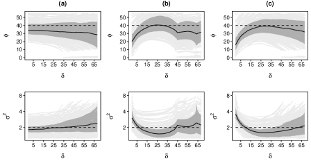
Figure 15 presents MMC estimates of parameters and against for scenario . We see a similar pattern to scenario , with the median of estimates for against from the simulated data (in (a)) decreasing until and staying approximately constant afterward. The median of estimated from the “randomly,” “positively,” and “negatively” corrupted data (as in(b)-(d)) have local maxima (i.e. what we take to be the optimal value of as discussed in ) at , and respectively. Figure 16 presents a comparison of estimates from different methods, as done in S1 and S2. We observe that the performance of MMC methods, especially for the estimation of , is equal to or better than other MC methods.

5 Application
We now revisit one of our motivating examples: Conflict events in Afghanistan using the SIGACTS and GED data. Figure 17 shows spatial point patterns from the SIGACTS and GED data sets, including spatial locations with duplicated data. We consider an inhomogeneous LGCP model for both data. We use the results from SIGACTS as the reference case since, as we discussed above, the location coordinates in SIGACTS are considered more accurate than the GED data. The adaptive kernel approach discussed in Section 3.3 is used to estimate the (highly heterogeneous) intensity for both SIGACTS and GED data. As we discussed in the simulation scenario , we use the OS approach to select the global bandwidth , which ends up at about 85 in this case. Additionally, we try two more choices, one smaller () and one larger (), to show the sensitivity of the MMC estimates to the choice of bandwidth.


Similar to the results in the simulation from Section 4, the MMC estimates of against for GED show local maxima (Figure 18). Moreover, as bandwidth increases, we see increases in both MC estimates for from SIGACTS (dashed lines) and MMC estimates for at optimal from GED, while optimal values are not sensitive to the choice of bandwidth. Therefore, for the rest of this section, we fix .
Figure 19 presents the estimated first-order intensity surfaces for SIGACTS, GED, and GED with three methods to handle the duplicates. We observe two high-intensity spots for the estimated intensity from SIGACTS, one in the east over the capital city (Kabul) and the other in the south of the country near Kandahar city. As expected, using the deletion method (\Romannum1), both “hot” spots are nearly absent, highlighting the degree of information loss that is a necessary consequence of this method. A comparison of estimates for and from different methods is presented in Figure 20. Compared to the reference estimates from SIGACTS, the proposed MMC method at optimal outperformed the other four methods. Although it is not our preferred approach, among currently available approaches in the literature, Method III performs the best in terms of the first- and second-order structures. As far as we can tell, this method has been introduced in the literature (Shi et al., 2013) as discussed in Section 2.1 but has not been fully utilized for the issue of duplicates or geo-location errors.


6 Discussion
In this study, we consider the challenges of analyzing and modeling spatial point patterns with duplicate points. Existing approaches to dealing with duplicate data often involve altering the original data, either removing duplicate observations or adding noise to reported locations. As an alternative, we advocate an approach that modifies the method of inference to account for duplicates, thereby preserving the integrity of the data. Using an LGCP model, we demonstrate how the MC method can be modified to account for duplicates by truncating the lower bound of integration in the discrepancy measure with a tuning parameter, . In doing so, only the less biased discrepancies are reflected in the estimation of the second-order parameters in the presence of duplicates. Using simulation experiments, we show that when duplicates result from the geo-coding process (that we call corruption), a natural choice for emerges to help guide the proposed MMC method. Typically, we find that the optimal is more a consequence of the data corruption process (e.g. the extent of the geo-location error) than the underlying spatial point pattern structure. Moreover, for both simulated and real-data applications, the MMC method with the optimal outperforms the general MC methods with existing approaches in handling duplicates. Where previous methods sought to obscure (jitter) or disregard (delete), our proposed method directly addresses the problem created by duplicates – the erroneous discrepancy at the micro-scale – by identifying where to begin measuring the true discrepancy.
While our approach offers improvements over existing ones to deal with duplicate data, several open questions remain that should guide future research. First, as an MC-based method, it inherits the problem of choice of tuning parameters such as , , and bandwidth for the empirical estimate of . Second, in some event datasets, there may be corruption at multiple spatial scales. As discussed above, the Global Terrorism Database has a “specificity” score indicating the level of resolution at which the data are snapped (e.g., the first-level administrative unit, the second-level administrative unit, etc.). In future work, we will consider how our proposed approach can be generalized to accommodate multiple levels of corruption structure. Finally, duplicates are only one issue caused by geo-location errors (i.e., inaccurate coordinate information) in event data. In future work, we plan to consider cases of more general geo-location errors and how our approach can be extended to account for them.
References
- Abramson (1982) Abramson, I. S. (1982), “On bandwidth variation in kernel estimates-a square root law,” The Annals of Statistics, 10, 1217–1223.
- Baddeley et al. (2007) Baddeley, A., Bárány, I., and Schneider, R. (2007), “Spatial point processes and their applications,” Stochastic Geometry: Lectures Given at the CIME Summer School Held in Martina Franca, Italy, September 13–18, 2004, 1–75.
- Baddeley et al. (2015) Baddeley, A., Rubak, E., and Turner, R. (2015), Spatial point patterns: methodology and applications with R, CRC Press.
- Baddeley et al. (2000) Baddeley, A. J., Møller, J., and Waagepetersen, R. (2000), “Non‐and semi‐parametric estimation of interaction in inhomogeneous point patterns,” Statistica Neerlandica, 54, 329–350.
- Buhaug and Gleditsch (2008) Buhaug, H. and Gleditsch, K. S. (2008), “Contagion or confusion? Why conflicts cluster in space,” International Studies Quarterly, 52, 215–233.
- Cederman and Gleditsch (2009) Cederman, L.-E. and Gleditsch, K. S. (2009), “Introduction to special issue on “disaggregating civil war”,” Journal of Conflict Resolution, 53, 487–495.
- Cook and Weidmann (2022) Cook, S. J. and Weidmann, N. B. (2022), “Race to the bottom: Spatial aggregation and event data,” International Interactions, 1–21.
- Cronie and van Lieshout (2018) Cronie, O. and van Lieshout, M. N. M. (2018), “A non-model-based approach to bandwidth selection for kernel estimators of spatial intensity functions,” Biometrika, 105, 455–462.
- Daley and Vere-Jones (2003) Daley, D. J. and Vere-Jones, D. (2003), An introduction to the theory of point processes: volume I: elementary theory and methods, Springer New York.
- Darmofal (2009) Darmofal, D. (2009), “Bayesian spatial survival models for political event processes,” American Journal of Political Science, 53, 241–257.
- Davies and Baddeley (2018) Davies, T. M. and Baddeley, A. (2018), “Fast computation of spatially adaptive kernel estimates,” Statistics and Computing, 28, 937–956.
- Davies and Hazelton (2013) Davies, T. M. and Hazelton, M. L. (2013), “Assessing minimum contrast parameter estimation for spatial and spatiotemporal log‐Gaussian Cox processes,” Statistica Neerlandica, 67, 355–389.
- Davies et al. (2018) Davies, T. M., Marshall, J. C., and Hazelton, M. L. (2018), “Tutorial on kernel estimation of continuous spatial and spatiotemporal relative risk,” Statistics in Medicine, 37, 1191–1221.
- Diggle (2003) Diggle, P. J. (2003), Statistical analysis of spatial point patterns, Arnold, London, 2nd ed.
- Diggle et al. (2013) Diggle, P. J., Moraga, P., Rowlingson, B., and Taylor, B. M. (2013), “Spatial and spatio-temporal log-Gaussian Cox processes: extending the geostatistical paradigm,” Statistical Science, 28, 542–563.
- Earl et al. (2004) Earl, J., Martin, A., McCarthy, J. D., and Soule, S. A. (2004), “The use of newspaper data in the study of collective action,” Annu. Rev. Sociol., 30, 65–80.
- GADM (2021) GADM (2021), “GADM database of Global Administrative Areas, version 4.1,” https://gadm.org/data.html. [Accessed: Jul 13, 2022].
- GeoNames (2023) GeoNames (2023), “All Cities with a population 1000,” https://download.geonames.org/export/dump/. [Accessed: Jan 23, 2023].
- Guan and Sherman (2007) Guan, Y. and Sherman, M. (2007), “On least squares fitting for stationary spatial point processes,” Journal of the Royal Statistical Society: Series B (Statistical Methodology), 69, 31–49.
- Heinrich (1992) Heinrich, L. (1992), “Minimum contrast estimates for parameters of ergodic spatial point processes,” Information Theory, Statistical Decision Functions, Random Processes: Transactions of the 11th Prague Conference Held from August 27 to 31, 1990, 479–492.
- Iftimi et al. (2018) Iftimi, A., van Lieshout, M.-C., and Montes, F. (2018), “A multi-scale area-interaction model for spatio-temporal point patterns,” Spatial Statistics, 26, 38–55.
- Jun and Cook (2024) Jun, M. and Cook, S. J. (2024), “Flexible multivariate spatio-temporal Hawkes process models of terrorism,” Annals of Applied Statistics, 18, 1378–1403.
- Krieger et al. (2015) Krieger, N., Chen, J. T., Waterman, P. D., Kiang, M. V., and Feldman, J. (2015), “Police killings and police deaths are public health data and can be counted,” PLoS Medicine, 12.
- LaFree (2019) LaFree, G. (2019), “The evolution of terrorism event databases,” in The Oxford Handbook of Terrorism, Oxford University Press, pp. 50–68.
- Lee et al. (2019) Lee, S. J., Liu, H., and Ward, M. D. (2019), “Lost in space: Geolocation in event data,” Political Science Research and Methods, 7, 871–888.
- Møller et al. (1998) Møller, J., Syversveen, A. R., and Waagepetersen, R. P. (1998), “Log Gaussian Cox processes,” Scandinavian Journal of Statistics, 25, 451–482.
- Møller and Waagepetersen (2017) Møller, J. and Waagepetersen, R. P. (2017), “Some recent developments in statistics for spatial point patterns,” Annual Review of Statistics and Its Application, 4, 317–342.
- Renner et al. (2015) Renner, I. W., Elith, J., Baddeley, A., Fithian, W., Hastie, T., Phillips, S. J., Popovic, G., and Warton, D. I. (2015), “Point process models for presence‐only analysis,” Methods in Ecology and Evolution, 6, 366–379.
- Ripley (1977) Ripley, B. D. (1977), “Modelling spatial patterns,” Journal of the Royal Statistical Society: Series B (Methodological), 39, 172–192.
- Shi et al. (2013) Shi, X., Miller, S., Mwenda, K., Onda, A., Rees, J., Onega, T., Gui, J., Karagas, M., Demidenko, E., and Moeschler, J. (2013), “Mapping disease at an approximated individual level using aggregate data: a case study of mapping New Hampshire birth defects,” International Journal of Environmental Research and Public Health, 10, 4161–4174.
- Silverman (1986) Silverman, B. W. (1986), Density estimation for statistics and data analysis, vol. 26, CRC Press.
- START (2021a) START (2021a), “Global Terrorism Database 1970 - 2020 [data file],” https://www.start.umd.edu/gtd.
- START (2021b) — (2021b), “Global Terrorism Database codebook: Methodology, inclusion criteria, and variables,” https://www.start.umd.edu/gtd/downloads/Codebook.pdf.
- Sundberg and Melander (2013) Sundberg, R. and Melander, E. (2013), “Introducing the UCDP georeferenced event dataset,” Journal of Peace Research, 50, 523–532.
- Terrell (1990) Terrell, G. R. (1990), “The maximal smoothing principle in density estimation,” Journal of the American Statistical Association, 85, 470–477.
- Tompson et al. (2015) Tompson, L., Johnson, S., Ashby, M., Perkins, C., and Edwards, P. (2015), “UK open source crime data: accuracy and possibilities for research,” Cartography and Geographic Information Science, 42, 97–111.
- Turner (2009) Turner, R. (2009), “Point patterns of forest fire locations,” Environmental and ecological statistics, 16, 197–223.
- Valente and Laurini (2023) Valente, F. and Laurini, M. (2023), “A spatio-temporal analysis of fire occurrence patterns in the Brazilian Amazon,” Scientific Reports, 13, 12727.
- Weidmann (2015) Weidmann, N. B. (2015), “On the accuracy of media-based conflict event data,” Journal of Conflict Resolution, 59, 1129–1149.
- World Bank Group (2019) World Bank Group (2019), “Afghanistan Road Network,” https://datacatalog.worldbank.org/search/dataset/0038673. [Accessed: Mar 22, 2023].
- WorldPop (2018) WorldPop (2018), “Global 1km Population,” https://www.worldpop.org. [Accessed: Jun 8, 2023].
- Zandbergen (2014) Zandbergen, P. A. (2014), “Ensuring confidentiality of geocoded health data: assessing geographic masking strategies for individual-level data,” Advances in Medicine, https://doi.org/10.1155/2014/567049.
- Zhu et al. (2021) Zhu, L., Cook, S. J., and Jun, M. (2021), “The promise and perils of point process models of political events,” ArXiv:2108.12566 [stat.ME].
Appendix A Varying levels of corruption in S1
Figure 21 shows the effect of different levels of corruption on the MMC estimates of against . As the corruption level increases, we observe that the black median curves deviate more from the median of MC estimates on uncorrupted data. Additionally, the cusps created by the regularity in the geometry of the grid become more apparent. Aside from these cusps, the deviation presents in both cases as an increase in the concavity of the median estimates.

Appendix B MC estimates against jittering radius
As shown in Figures 22 and 23, for both simulated and GED data, the median of estimated curves for both and exhibit monotonic responses to jittering radius, leaving no clear optimality condition.


Appendix C Optimal bandwidths based on RED criterion
As shown at the top of Figure 24, for , as fixed bandwidth increases, estimated increases while estimated decreases. On the other hand, the bottom of the figure shows that in , parameter estimates are not stable (i.e. have wide uncertainty bounds) at small bandwidths. But after the bounds stabilize, and we see a clear upward trend with and roughly constant . The RED curves have global minima for both and , which provides an optimal bandwidth.


Appendix D Supplementary Figures for S3


