Conformal Classification with Equalized Coverage for Adaptively Selected Groups
Abstract
This paper introduces a conformal inference method to evaluate uncertainty in classification by generating prediction sets with valid coverage conditional on adaptively chosen features. These features are carefully selected to reflect potential model limitations or biases. This can be useful to find a practical compromise between efficiency—by providing informative predictions—and algorithmic fairness—by ensuring equalized coverage for the most sensitive groups. We demonstrate the validity and effectiveness of this method on simulated and real data sets.
1 Introduction
1.1 Uncertainty, Fairness, and Efficiency in Machine Learning
Increasingly sophisticated machine learning (ML) models, like deep neural networks, are revolutionizing decision-making in many high-stakes domains, including medical diagnostics [1], job screening [2], and recidivism prediction [3, 4]. However, serious concerns related to uncertainty quantification [5, 6] and algorithmic fairness [7, 8, 9, 10] underscore the need for novel methods that can provide reliable and unbiased measures of confidence, applicable to any model.
Uncertainty quantification is crucial because ML models, although effective on average, can make errors while displaying overconfidence [11]. Consequently, in some situations users may lack sufficient warning about the potential unreliability of a prediction, raising trust and safety concerns. A promising solution is conformal inference [12, 13, 14], which enables converting the output of any model into prediction sets with precise coverage guarantees. These sets reflect the model’s confidence on a case-by-case basis, with smaller sets indicating higher confidence in a specific prediction.
Algorithmic fairness focuses on the challenges of prediction inaccuracies that disproportionately impact specific groups, often identified by sensitive attributes like race, sex, and age. Among the many sources of algorithmic bias are training data that do not adequately represent the population’s heterogeneity and a focus on maximizing average performance. However, fairness is partly subjective and lacks a universally accepted definition [15], leading to sometimes conflicting interpretations [16].
This complexity makes conformal inference with equalized coverage [17] an appealing approach. Equalized coverage aims to ensure that the prediction sets attain their coverage not only on average for the whole population (e.g., above 90%) but also at the same level within each group of interest. While this does not necessarily imply that the prediction sets will have equal size on average across different groups—since it is possible the predictive model may be more or less accurate for different groups—it objectively communicates the possible limitations of a model.
The rationale for conformal inference with equalized coverage is twofold. First, it is more straightforward compared to correcting a model’s inaccuracies, which may require retraining with better data or imposing constraints that deviate from a data-driven approach. Second, it is beneficial because reliable uncertainty estimates can mitigate the negative impact of over-reliance on potentially inaccurate predictions. Thus, this approach maintains data integrity while enhancing fairness and reliability.
A limitation of the current method for conformal inference with equalized coverage is that it does not scale well to situations involving diverse populations with multiple sensitive attributes. In such cases, it necessitates splitting the data into exponentially many subsets, significantly reducing the effective sample size and leading to less informative predictions. Balancing this trade-off [18] between efficiency—aiming for highly informative predictions—and fairness—ensuring unbiased treatment—is challenging and requires novel approaches. This paper introduces a method to address this by providing equalized coverage conditional on carefully chosen features, informed by the model and data. While it cannot guarantee equalized coverage for all sensitive groups, it seeks a reasonable compromise with finite data sets, mitigating significant biases while retaining predictive power.
1.2 Background on Conformal Inference for Classification
Consider a data set comprising exchangeable (e.g., i.i.d.) observations for , sampled from an arbitrary and unknown distribution . In classification, one can write , where is a categorical label and represents the individual’s features, taking values in some space . As explained below, we will assume these features include some sensitive attributes. Further, we consider a test point , also sampled exchangeably from , and whose label has not yet been observed.
A standard goal for split conformal prediction methods is to quantify the predictive uncertainty of a given “black-box” ML model (e.g., pre-trained on an independent data set) by constructing a prediction set for , guaranteeing marginal coverage at some desired level :
| (1) |
Above, the probability is taken over the randomness in both and , as well as in the data indexed by . Intuitively, marginal coverage means that the prediction sets are expected to cover the correct outcomes for a fraction of the population. However, this is not always satisfactory, especially if one is concerned that the miscoverage errors may disproportionately affect individuals characterized by well-defined features.
To address these concerns, one might consider feature-conditional coverage, for all . This would ensure consistent coverage for all possible test features . However, it is impossible to achieve without additional assumptions, such as modeling the distribution [19] or significantly restricting the feature space [20]. Given that such assumptions may be unrealistic in real-world settings, exact feature-conditional coverage is typically unachievable.
Equalized coverage [17] seeks a practical middle ground between the two extremes of marginal and feature-conditional coverage, focusing on accounting for specific discrete attributes encapsulated by . To facilitate the subsequent exposition of our method, it is useful to recall the definition of equalized coverage with the following notation.
Let denote the number of sensitive attributes, and for each let count the possible values of the -th attribute. Consider a function , so that for each subset of attribute indices, is a vector of length representing the values of all attributes indexed by for an individual with features . In the special case where is a singleton, e.g., for some , then denotes the value of the -th attribute; e.g., someone’s race. More generally, , for any distinct , denotes the joint values of two attributes, characterizing a smaller group like “Asian Males”.
The notion of exhaustive equalized coverage, introduced by [17] and termed “exhaustive” here to distinguish it from other possible related notions, is defined as:
| (2) |
In words, this says has valid coverage conditional on all sensitive attributes. Prediction sets satisfying (2) can be obtained by applying the standard conformal calibration method separately within each of the groups characterized by a specific combination of the protected attributes represented by ; see Appendix A1 for details. However, a downside of this approach is that the calibration subsets may be too small if is large, leading to uninformative predictions for even moderate values of . This limitation forms the starting point of our work.
1.3 Preview of Our Contributions: Adaptive Equalized Coverage
In practice, for a given model and data set, different groups may not exhibit the same need for rigorous equalized coverage guarantees (2), as conformal predictions may be able to approximately achieve the desired coverage even without explicit constraints. Algorithmic bias typically affects only a minority of the population, so standard prediction sets with marginal coverage (1) may approximately satisfy (2) for most groups. Therefore, we propose Adaptively Fair Conformal Prediction (AFCP), a new method that efficiently identifies and addresses groups suffering from algorithmic bias in a data-driven way, adjusting their prediction sets to equalize coverage without sacrificing informativeness.
AFCP involves two main steps. First, as sketched in Figure 1, it carefully selects a sensitive attribute , based on and the data in . Although AFCP can be extended to select multiple attributes, we begin by focusing on this simpler version for clarity. Intuitively, AFCP searches for the attribute corresponding to the group most negatively affected by algorithmic bias. It may also opt to select no attribute () in the absence of significant biases.
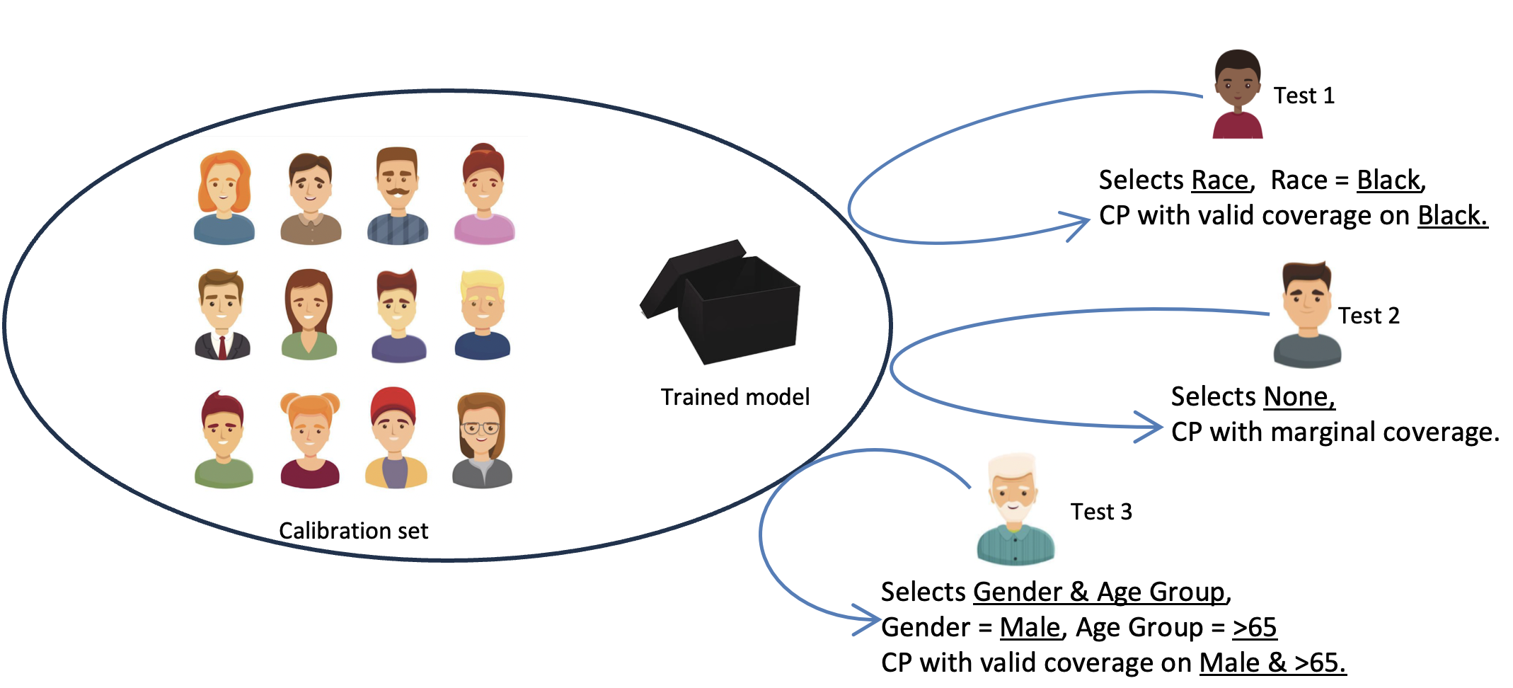
Next, AFCP constructs a prediction set for that guarantees the following notion of adaptive equalized coverage at the desired level :
| (3) |
In words, this tells us is well-calibrated for the groups defined by the selected attribute . It is worth highlighting the key distinctions between (3) and the existing notions of coverage reviewed above. On the one hand, if AFCP identifies no significant bias, selecting , then (3) reduces to marginal coverage (1), following the convention that is a constant. On the other hand, exhaustive equalized coverage (2) would correspond to simultaneously selecting all possible sensitive attributes instead of only that identified by . To clarify the terminology, in this paper we will say that an attribute is sensitive if it may identify a group affected by algorithmic bias. By contrast, a protected attribute is one for which equalized coverage is explicitly sought.
Figure 2 illustrates this intuition through a simulated example. In this scenario, we generate synthetic medical diagnosis data, considering six possible diagnosis labels, and designate race, sex, and age group as potentially sensitive attributes alongside other demographic factors. Notably, the Black group, identified by race, is characterized by fewer samples and higher algorithmic bias, resulting in marginal prediction sets with low group-conditional coverage. By contrast, the model leads to no significant disparities across the sexes and age groups in this dataset.
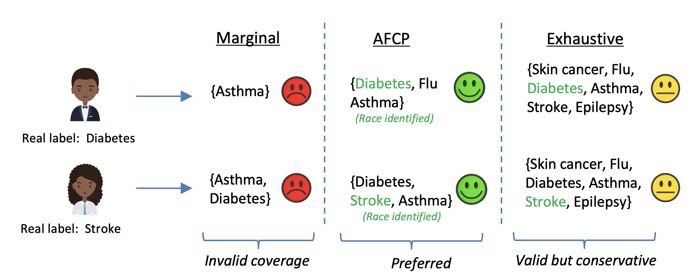
For two example patients from the critical group, the standard marginal prediction sets fail to cover the true label. Conversely, sets calibrated for exhaustive equalized coverage are too conservative to be informative. By contrast, AFCP generates prediction sets that are both efficient and fair.
Without additional sample splitting, which would be inefficient, constructing informative prediction sets that satisfy (3) is challenging due to potential selection bias from using the same data for attribute selection and conformal calibration. This paper presents a novel solution to address this challenge.
1.4 Table of Contents
Section 2 presents our AFCP method, focusing on the special case in which at most one sensitive attribute may be selected. Section 3 demonstrates the empirical performance of AFCP on synthetic and real data. Section 4 discusses some limitations and suggests ideas for future work.
Additional content is presented in the Appendices. Appendix A1 reviews relevant details of existing approaches. Appendices A2 and A3 present two extensions of our method, respectively enabling the selection of more than one sensitive attribute and providing valid coverage also conditional on the true test label; both extensions involve distinct technical challenges. Additionally, a variation of AFCP designed for outlier detection tasks is detailed in Appendix A4. Appendix A5 contains all mathematical proofs. Appendix A6 explains how to implement our method efficiently and studies its computational cost. Appendix A7 describes the results of numerous additional experiments.
1.5 Related Works
Conformal inference is a very active research area, with numerous methods addressing diverse tasks, including outlier detection [21, 22, 23], classification [24, 25, 26, 27, 28], and regression [29, 30, 31]. Overcoming the limitations of the standard marginal coverage guarantees (1) is a main interest in this field.
Some works have proposed conformity scores designed to seek high feature-conditional coverage while calibrating prediction sets for marginal coverage [30, 27]. Others attempt to mitigate overconfidence while training the ML model [32, 33], and several have developed calibration methods for non-exchangeable data, accounting for possible distribution shifts [34, 35, 36, 37, 38]. These works are complementary to ours, as we focus on guaranteeing a new adaptive notion of equalized coverage.
In addition to [17], several other works have considered constructing prediction sets adhering to various notions of equalized coverage and have empirically investigated the performance of conformal predictors in this regard [39]. In the context of regression, [40] and [41] proposed strategies to enhance conditional coverage given several protected attributes, but they targeted a different notion of equalized coverage designed for continuous outcomes. In classification, a classical approach to move beyond marginal coverage is label-conditional coverage, where the “protected” groups are defined not based on the features but by the label itself, [42, 43, 44]. As explained in Appendix A3, the method proposed in this paper can also be extended to provide label-conditional coverage.
More closely related to the notion of equalized coverage [17] are the works of [45, 46], which differ from ours as they do not consider the automatic selection of the sensitive groups. To tackle a related challenge due to unknown biased attributes, [47] studied how to identify unfairly treated groups by establishing a simultaneously valid confidence bound on group-wise disparities. In principle, their approach can be integrated within the selection component of our method. Very recently, [48] proposed an elegant method to obtain valid conformal prediction sets for adaptively selected subsets of test cases. While their perspective aligns more closely with ours, their approach and focus differ as they study different selection rules not specifically aimed at mitigating algorithmic bias.
2 Method
2.1 Automatic Attribute Selection
Given a pre-trained classifier, an independent calibration data set , and a test point with an unknown label , we will select (at most) one sensitive attribute, , according to the following leave-one-out procedure.
For each , imagine is equal to , and define an augmented calibration set . For each , define also the leave-one-out set , with acting as a placeholder for . Then, for each , we construct a conformal prediction set for given by calibrating the classifier using the data in . Any method can be applied for this purpose, although it may be helpful for concreteness to focus on employing the standard approach seeking marginal coverage (1) using the adaptive conformity scores proposed by [27]. Let denote the binary indicator of whether fails to cover :
| (4) |
After evaluating for all , we will assess the leave-one-out miscoverage rate for the worst-off group identified by each sensitive attribute . That is, we evaluate
Intuitively, denotes the maximum miscoverage rate across all groups identified by the -th attribute. Large values of suggest that the -th attribute may be a sensitive attribute corresponding to at least one group suffering from algorithmic bias.
To assess whether there is evidence of significant algorithmic bias, we can perform a statistical test for the null hypothesis that no algorithmic bias exists. Note that this test can be heuristic since it does not need to be exact for our method to rigorously guarantee (3). Therefore, we do not need to carefully consider the assumptions underlying this test. As a useful heuristic, we define:
| (5) |
and carry out a one-sided t-test for the null hypothesis against .
If is rejected (at any desired level, like 5%), we conclude there exists a group suffering from significant algorithmic bias, and we identify the corresponding attribute through
| (6) |
Otherwise, we set , which corresponds to selecting no attribute. See Algorithm 1 for an outline of this procedure, as a function of the placeholder label .
After repeating this procedure for each , the final selected attribute is:
| (7) |
Therefore, an attribute is selected if and only if it is consistently flagged by our leave-one-out procedure for all values of the placeholder label . This approach minimizes the potential arbitrariness due to the use of a placeholder label and is necessary to guarantee that our method constructs prediction sets achieving (3), as discussed in the next section.
Before explaining how our method utilizes the selected sensitive attribute obtained in (7) to construct prediction sets satisfying (3), we pause to make two remarks. First, as long as is large enough, is quite stable with respect to both and , as each of these variables plays a relatively small role in determining the leave-one-out miscoverage rates. Therefore, the selected attribute given by (7) is also quite stable for different values of . This stability will be demonstrated empirically in Section 3. Second, despite its iterative nature, our method can be implemented efficiently; see Appendix A6. Further, if is very large, our method could be streamlined using cross-validation instead of a leave-one-out approach.
2.2 Constructing the Adaptive Prediction Sets
After evaluating by applying Algorithm 1 with placeholder label for for all , and selecting a (possibly empty) subset of attributes using (7), AFCP constructs an adaptive prediction set for that satisfies (3) as follows.
First, it constructs a marginal conformal prediction set targeting (1), by applying the standard approach reviewed in Appendix A1. Then, for each , it constructs a conformal prediction set with equalized coverage for the group identified by attribute , as if it had been fixed. This is achieved by applying the standard marginal method based on a restricted calibration sample indexed by ; see Algorithm A1 in Appendix A1 for further details. Therefore, note that becomes equivalent to if . Finally, the AFCP prediction set for is given by:
| (8) |
See Algorithm 2 for an outline of this procedure.
Note that the AFCP set given by (8) always contains the marginal set ; this is essential to prove the validity of our approach. Second, in practice the selection tends to be very consistent for different values of the placeholder label , as long as the sample size is large enough; therefore, the union in (8) will typically not lead to a very large prediction set.
The following result, proved in Appendix A5, establishes that the prediction sets output by AFCP guarantee adaptive equalized coverage (3) with respect to the adaptively selected attribute . It is worth emphasizing this result is not straightforward and involves an innovative proof technique to address the lack of exchangeability introduced by the adaptive selection step.
3 Numerical Experiments
3.1 Setup and Benchmarks
This section demonstrates the empirical performance of AFCP, focusing on the implementation described in Section 2, which selects at most one sensitive attribute. Our method is compared with three existing approaches, which utilize the same data, ML model, and conformity scores but produce prediction sets with different guarantees. The first is the marginal benchmark, which constructs prediction sets guaranteeing (1) by applying Algorithm A1 without protected attributes. The second is the exhaustive equalized benchmark, which constructs prediction sets guaranteeing (2) by applying Algorithm A1 with all sensitive attributes simultaneously protected. The third is a partial equalized benchmark that separately applies Algorithm A1 with each possible protected attribute , and then takes the union of all such prediction sets. This is an intuitive approach that can be easily verified to provide a coverage guarantee intermediate between (2) and (3), namely:
| (9) |
However, we will see that these prediction sets are often still too conservative in practice.
In addition, we apply a variation of AFCP that always selects one sensitive attribute, regardless of the outcome of the significance test. This method is denoted as AFCP1 in our experiments.
For all methods considered, the classifier is based on a five-layer neural network with linear layers interconnected via a ReLU activation function. The output layer uses a softmax function to estimate the conditional label probabilities. The Adam optimizer and cross-entropy loss function are used in the training process, with a learning rate set at 0.0001. The loss values demonstrate convergence after 100 epochs of training. For all methods, the miscoverage target level is set at .
3.2 Synthetic Data
We generate synthetic classification data to mimic a medical diagnosis task with six possible labels: Skin cancer, Diabetes, Asthma, Stroke, Flu, and Epilepsy. The available features include three sensitive attributes—Age Group, Region, and Color—and six additional non-sensitive covariates. Color is categorized as Blue or Grey, with 10% and 90% marginal frequencies, respectively. The Age Group is cyclically repeated as , and Region is sampled from an i.i.d. multinomial distribution across with equal probabilities. The six non-sensitive features are i.i.d. random samples from a uniform distribution on . For simplicity, Color is denoted as and the first non-sensitive feature as . Conditional on , the label is generated based on a decision tree model that depends only on and , as detailed in Appendix A7. This model is designed so that the diagnosis label for individuals with Color equal to Blue is intrinsically harder to predict, mimicking the presence of algorithmic bias.
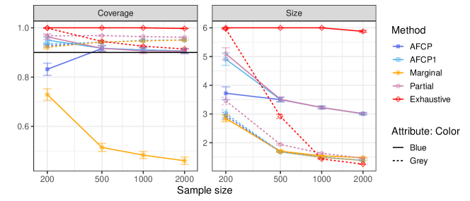
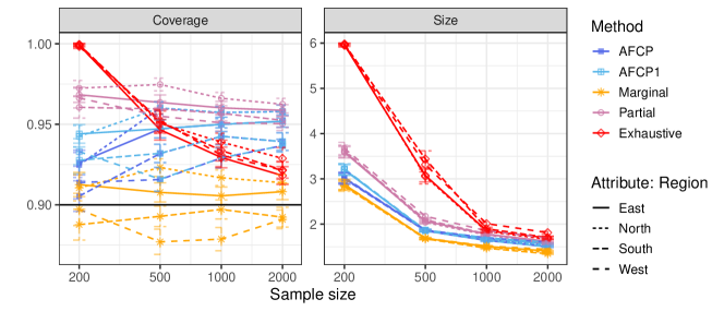
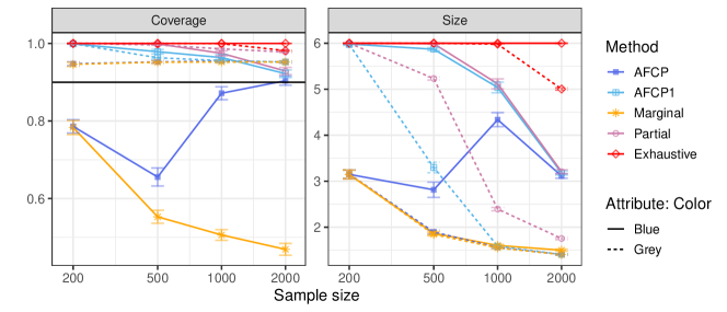
Figure 3 shows the performance of all methods as a function of the total sample size, ranging from 200 to 2000. In each case, of the samples are used for training and the remaining for calibration. Results are averaged over 500 test points and 100 independent experiments.
While the marginal benchmark produces the smallest prediction sets on average, it leads to significant empirical undercoverage within the Blue group. In contrast, the exhaustive benchmark, which achieves the highest coverage overall, tends to lead to overly conservative and thus uninformative prediction sets, especially for the Blue group. The partial benchmark, though less conservative than the exhaustive method, still generates prediction sets that are too large when the sample size is small.
Our AFCP method and its simpler variation, AFCP1, not only achieve valid coverage for the Blue group but do so with prediction sets that, on average, are not much larger than the marginal ones. AFCP1 is slightly more robust than AFCP when the sample size is very small, as it never fails to select a sensitive attribute. This is advantageous in scenarios where we know there is a sensitive attribute worth equalizing coverage for, though this may not always be the case in practice. See Figure A1 and Table A1 for detailed results with standard errors.

Figure 4 provides additional insight into our method’s performance by plotting the selection frequencies of each sensitive attribute as a function of sample size, within the same experiments described in Figure 3. These results show that our method behaves as anticipated. When the sample size and algorithmic bias are both small, AFCP shows more variability in selecting the sensitive attribute, often selecting no attributes. However, as the sample size grows and the undercoverage affecting the Blue group becomes more pronounced, AFCP consistently selects Color as the most sensitive attribute, correctly identifying the main manifestation of algorithmic bias in these data.

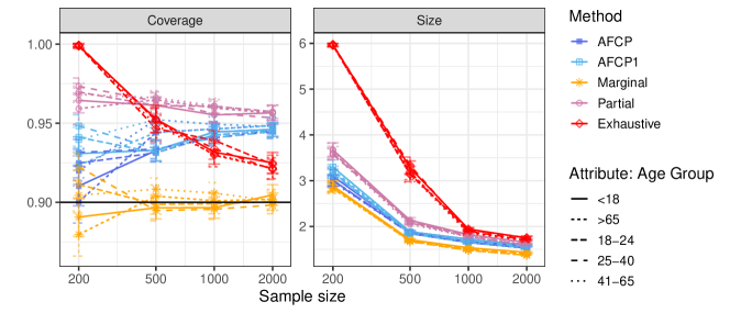
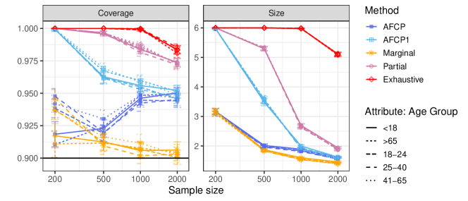
Additional results are presented in Appendix A7.1.1. Figures A1–A3 and Tables A2–A4 summarize the average coverage and prediction set size conditional on each protected attribute. Figures A4–A7 and Tables A5–A8 study the performance of an extension of our method that also provides valid coverage conditional on the true label of the test point.
3.3 Nursery data
We apply AFCP and its benchmarks to the open-domain Nursery data set [49], which was derived from a hierarchical decision model originally developed to rank applications for nursery schools for social science studies. The data encompass 12,960 instances with eight categorical features: Parents’ occupation (3 levels), Child’s nursery (5 levels), Family form (4 levels), Number of children (1, 2, 3, or more), Housing conditions (3 levels), Financial standing (2 levels), Social conditions (3 levels), and Health status (3 levels). These features are used to predict application ranks across five categories. The variables “Parents’ occupation", “Number of children", “Financial standing", “Social conditions", and “Health status" are marked as possible sensitive attributes.
To prepare for model training, we executed several pre-processing steps. First, two instances labeled “recommend" were removed due to the minimal occurrence of this outcome label. Subsequently, we utilized the LabelEncoder function in the sklearn Python package to numerically encode all features and labels. To make the problem more interesting and allow control over the strength of algorithmic bias, we added independent, uniformly distributed noise to the labels of samples with Parents’ occupation in the first category, rounding these perturbed labels to the nearest integer. This makes the group corresponding to the first category of Parents’ occupation intrinsically more unpredictable and hence more prone to algorithmic bias. To enhance the challenge of making accurate predictions for this group, it was further down-sampled to 10% of its original size.
Figure 5 summarizes the performance of all approaches as a function of the total number of training and calibration data points, which varies between 200 and 5000. The results are averaged over 500 randomly chosen test points and 100 repeated experiments. In each experiment, 50% of the samples are randomly assigned for training and the remaining 50% for calibration. The marginal benchmark is heavily biased, leading to prediction sets with very low coverage for samples with Parents’ occupation in the first category. The exhaustive benchmark is too conservative and results in very large prediction sets unless the sample size is very large. The partial benchmark performs better than the other two benchmarks, but our AFCP method still outperforms it, producing smaller prediction sets with valid coverage even for the hardest-to-predict group. See Table A9 for detailed results.

The results of additional experiments are presented in Appendix A7.1.2. Figures A8–A12 and Tables A10–A14 detail the average coverage and prediction set size for each sensitive attribute. Additionally, Figures A13–A18 and Tables A15–A20 report on the performance of an extended version of AFCP which also ensured valid coverage conditional on the true test label.
3.4 Additional Numerical Experiments
4 Discussion
This paper presents a practical and statistically principled method to construct informative conformal prediction sets with valid coverage conditional on adaptively selected features. This approach balances efficiency and equalized coverage, which may be particularly useful in applications involving multiple sensitive attributes. While we believe it offers substantial benefits, a potential limitation of this method is that it does not always identify the most relevant sensitive attribute, particularly when working with limited sample sizes. Nevertheless, our empirical results are quite encouraging, demonstrating that AFCP effectively mitigates significant instances of algorithmic bias when the sample size is adequate. Moreover, our method is flexible, allowing for the integration of prior knowledge about which sensitive attributes might require protection against algorithmic bias.
This paper creates several opportunities for further work. Future research could focus on theoretically studying the conditions under which our method can be guaranteed to select the correct sensitive attribute with high probability. Additionally, future extensions might explore implementing different attribute selection procedures, such as those inspired by [47]. Finally, extending our method to accommodate regression tasks with continuous outcomes presents additional computational challenges, but potential solutions could be inspired by [33].
The numerical experiments described in this paper were carried out on a computing cluster. Individual experiments, involving 1000 calibration samples and 500 test samples, required less than 25 minutes and 5GB of memory on a single CPU. The entire project took approximately 100 hours of computing time, and did not involve preliminary or failed experiments.
References
- Jones et al. [2020] A. Jones, B. Smith, and C. Johnson. Deep learning models for medical diagnosis. Journal of Medical Imaging, 7(2):021008, 2020.
- Brown et al. [2021] J. K. Brown et al. Using machine learning for job application screening: A comparative analysis. In International Conference on Artificial Intelligence in HR, pages 12–21, 2021.
- Zeng et al. [2017] Jiaming Zeng, Berk Ustun, and Cynthia Rudin. Interpretable classification models for recidivism prediction. J. R. Stat. Soc. (A), 180(3):689–722, 2017.
- Kuchibhotla and Berk [2023] Arun K Kuchibhotla and Richard A Berk. Nested conformal prediction sets for classification with applications to probation data. Ann. Appl. Stat., 17(1):761–785, 2023.
- Nguyen et al. [2015] Anh Nguyen, Jason Yosinski, and Jeff Clune. Deep neural networks are easily fooled: High confidence predictions for unrecognizable images. In IEEE Conference on Computer Vision and Pattern Recognition, pages 427–436, 2015.
- Guo et al. [2017] Chuan Guo, Geoff Pleiss, Yu Sun, and Kilian Q Weinberger. On calibration of modern neural networks. In Int. Conf. Mach. Learn., pages 1321–1330. PMLR, 2017.
- Dwork et al. [2012] Cynthia Dwork, Moritz Hardt, Toniann Pitassi, Omer Reingold, and Richard Zemel. Fairness through awareness. In Innovations in Theoretical Computer Science Conference, page 214–226. Association for Computing Machinery, 2012.
- Zemel et al. [2013] Richard Zemel, Yu (Ledell) Wu, Kevin Swersky, Toniann Pitassi, and Cyntia Dwork. Learning fair representations. In Int. Conf. Mach. Learn., 2013.
- Hardt et al. [2016] Moritz Hardt, Eric Price, Eric Price, and Nati Srebro. Equality of opportunity in supervised learning. In Adv. Neural. Inf. Process. Syst., volume 29, 2016.
- Berk et al. [2021] Richard A Berk, Arun Kumar Kuchibhotla, and Eric Tchetgen Tchetgen. Improving fairness in criminal justice algorithmic risk assessments using optimal transport and conformal prediction sets. Sociological Methods & Research, 2021.
- Ovadia et al. [2019] Yaniv Ovadia, Emily Fertig, Jie Ren, Zachary Nado, David Sculley, Sebastian Nowozin, Joshua Dillon, Balaji Lakshminarayanan, and Jasper Snoek. Can you trust your model’s uncertainty? evaluating predictive uncertainty under dataset shift. Adv. Neural Inf. Process. Syst., 32, 2019.
- Papadopoulos et al. [2002] Harris Papadopoulos, Kostas Proedrou, Vladimir Vovk, and Alex Gammerman. Inductive confidence machines for regression. In Eur. Conf. Mach. Learn., pages 345–356, 2002.
- Vovk et al. [2005] Vladimir Vovk, Alex Gammerman, and Glenn Shafer. Algorithmic learning in a random world. Springer, 2005.
- Lei et al. [2018] Jing Lei, Max G’Sell, Alessandro Rinaldo, Ryan J. Tibshirani, and Larry Wasserman. Distribution-free predictive inference for regression. J. Am. Stat. Assoc., 113(523):1094–1111, 2018.
- Hellman [2020] Deborah Hellman. Measuring algorithmic fairness. Virginia Law Review, 106(4):811–866, 2020.
- Chouldechova [2017] Alexandra Chouldechova. Fair prediction with disparate impact: A study of bias in recidivism prediction instruments. Big Data, 5(2):153–163, 2017.
- Romano et al. [2020a] Yaniv Romano, Rina Foygel Barber, Chiara Sabatti, and Emmanuel Candès. With malice toward none: Assessing uncertainty via equalized coverage. Harvard Data Science Review, 2020a.
- Fan et al. [2023] Jianqing Fan, Xin Tong, Yanhui Wu, and Shunan Yao. Neyman-Pearson and equal opportunity: when efficiency meets fairness in classification. arXiv preprint arXiv:2310.01009, 2023.
- Barber et al. [2021] Rina Foygel Barber, Emmanuel J Candès, Aaditya Ramdas, and Ryan J Tibshirani. The limits of distribution-free conditional predictive inference. Information and Inference, 10(2):455–482, 2021.
- Lee and Barber [2021] Yonghoon Lee and Rina Barber. Distribution-free inference for regression: discrete, continuous, and in between. Adv. Neural Inf. Process. Syst., 34:7448–7459, 2021.
- Bates et al. [2023] Stephen Bates, Emmanuel Candès, Lihua Lei, Yaniv Romano, and Matteo Sesia. Testing for outliers with conformal p-values. Ann. Stat., 51(1):149 – 178, 2023.
- Marandon et al. [2024] Ariane Marandon, Lihua Lei, David Mary, and Etienne Roquain. Adaptive novelty detection with false discovery rate guarantee. Ann. Stat., 52(1):157–183, 2024.
- Liang et al. [2024a] Ziyi Liang, Matteo Sesia, and Wenguang Sun. Integrative conformal p-values for out-of-distribution testing with labelled outliers. J. R. Stat. Soc. (B), page qkad138, 2024a.
- Lei et al. [2013] Jing Lei, James Robins, and Larry Wasserman. Distribution-free prediction sets. J. Am. Stat. Assoc., 108(501):278–287, 2013.
- Sadinle et al. [2019] Mauricio Sadinle, Jing Lei, and Larry Wasserman. Least ambiguous set-valued classifiers with bounded error levels. J. Am. Stat. Assoc., 114(525):223–234, 2019.
- Podkopaev and Ramdas [2021] Aleksandr Podkopaev and Aaditya Ramdas. Distribution-free uncertainty quantification for classification under label shift. In Uncertainty in Artificial Intelligence, pages 844–853. PMLR, 2021.
- Romano et al. [2020b] Yaniv Romano, Matteo Sesia, and Emmanuel J. Candès. Classification with valid and adaptive coverage. Adv. Neural Inf. Process. Syst., 33, 2020b.
- Angelopoulos et al. [2021] Anastasios Nikolas Angelopoulos, Stephen Bates, Michael Jordan, and Jitendra Malik. Uncertainty sets for image classifiers using conformal prediction. In Int. Conf. Learn. Represent., 2021.
- Lei and Wasserman [2014] Jing Lei and Larry Wasserman. Distribution-free prediction bands for non-parametric regression. J. R. Stat. Soc. (B), 76(1):71–96, 2014.
- Romano et al. [2019] Yaniv Romano, Evan Patterson, and Emmanuel J Candès. Conformalized quantile regression. In Adv. Neural Inf. Process. Syst., pages 3538–3548, 2019.
- Sesia and Romano [2021] Matteo Sesia and Yaniv Romano. Conformal prediction using conditional histograms. Adv. Neural Inf. Process. Syst., 34, 2021.
- Einbinder et al. [2022] Bat-Sheva Einbinder, Yaniv Romano, Matteo Sesia, and Yanfei Zhou. Training uncertainty-aware classifiers with conformalized deep learning. In Adv. Neural Inf. Process. Syst., volume 35, 2022.
- Liang et al. [2023] Ziyi Liang, Yanfei Zhou, and Matteo Sesia. Conformal inference is (almost) free for neural networks trained with early stopping. In Int. Conf. Mach. Learn., 2023.
- Barber et al. [2023] Rina Foygel Barber, Emmanuel J Candès, Aaditya Ramdas, and Ryan J Tibshirani. Conformal prediction beyond exchangeability. Ann. Stat., 51(2):816–845, 2023.
- Tibshirani et al. [2019] Ryan J Tibshirani, Rina Foygel Barber, Emmanuel Candès, and Aaditya Ramdas. Conformal prediction under covariate shift. Adv. Neural Inf. Process. Syst., 32, 2019.
- Gibbs and Candès [2022] Isaac Gibbs and Emmanuel Candès. Conformal inference for online prediction with arbitrary distribution shifts. arXiv preprint arXiv:2208.08401, 2022.
- Yang et al. [2024] Yachong Yang, Arun Kumar Kuchibhotla, and Eric Tchetgen Tchetgen. Doubly robust calibration of prediction sets under covariate shift. J. R. Stat. Soc. (B), page qkae009, 2024.
- Liang et al. [2024b] Ziyi Liang, Tianmin Xie, Xin Tong, and Matteo Sesia. Structured conformal inference for matrix completion with applications to group recommender systems. arXiv preprint arXiv:2404.17561, 2024b.
- Lu et al. [2022] Charles Lu, Andreanne Lemay, Ken Chang, Katharina Hoebel, and Jayashree Kalpathy-Cramer. Fair conformal predictors for applications in medical imaging. AAAI Conference on Artificial Intelligence, 36:12008–12016, 06 2022.
- Wang et al. [2023] Fangxin Wang, Lu Cheng, Ruocheng Guo, Kay Liu, and Philip S. Yu. Equal opportunity of coverage in fair regression. In Adv. Neural Inf. Process. Syst, 2023.
- Liu et al. [2022] Meichen Liu, Lei Ding, Dengdeng Yu, Wulong Liu, Linglong Kong, and Bei Jiang. Conformalized fairness via quantile regression. In Alice H. Oh, Alekh Agarwal, Danielle Belgrave, and Kyunghyun Cho, editors, Adv. Neural Inf. Process. Syst., 2022.
- Vovk et al. [2003] Vladimir Vovk, David Lindsay, Ilia Nouretdinov, and Alex Gammerman. Mondrian confidence machine. Technical report, Royal Holloway, University of London, 2003. On-line Compression Modelling project.
- Ding et al. [2024] Tiffany Ding, Anastasios Angelopoulos, Stephen Bates, Michael Jordan, and Ryan J Tibshirani. Class-conditional conformal prediction with many classes. Adv. Neural Inf. Process. Syst., 36, 2024.
- Löfström et al. [2015a] Tuve Löfström, Henrik Boström, Henrik Linusson, and Ulf Johansson. Bias reduction through conditional conformal prediction. Intell. Data Anal., 19(6):1355–1375, nov 2015a. ISSN 1088-467X.
- Jung et al. [2023] Christopher Jung, Georgy Noarov, Ramya Ramalingam, and Aaron Roth. Batch multivalid conformal prediction. In Int. Conf. Learn. Represent., 2023.
- Gibbs et al. [2023] Isaac Gibbs, John J Cherian, and Emmanuel J Candès. Conformal prediction with conditional guarantees. arXiv preprint arXiv:2305.12616, 2023.
- Cherian and Candès [2023] John J. Cherian and Emmanuel J. Candès. Statistical inference for fairness auditing. arXiv preprint arXiv:2305.03712, 2023.
- Jin and Ren [2024] Ying Jin and Zhimei Ren. Confidence on the focal: Conformal prediction with selection-conditional coverage. arXiv preprint arXiv:2403.03868, 2024.
- Rajkovic [1997] Vladislav Rajkovic. Nursery. UCI Machine Learning Repository, 1997. DOI: https://doi.org/10.24432/C5P88W, License: CC-BY 4.0.
- Becker and Kohavi [1996] Barry Becker and Ronny Kohavi. Adult. UCI Machine Learning Repository, 1996. DOI: https://doi.org/10.24432/C5XW20, License: CC-BY 4.0.
- Shafer and Vovk [2008] Glenn Shafer and Vladimir Vovk. A tutorial on conformal inference. J. Mach. Learn. Res., 9(3), 2008.
- Löfström et al. [2015b] Tuve Löfström, Henrik Boström, Henrik Linusson, and Ulf Johansson. Bias reduction through conditional conformal prediction. Intell. Data Anal., 19(6):1355–1375, 11 2015b.
Appendix A1 Review of Existing Conformal Classification Methods
Algorithm A1 outlines the standard approach for constructing conformal prediction sets with equalized coverage with respect to a fixed list of protected attributes [17]. In the special case where the list of protected attributes is empty, this method reduces to the standard approach for constructing prediction sets with marginal coverage.
In the context of outlier detection, Algorithm A2 reviews the standard approach for computing conformal p-values achieving valid false positive rate (FPR) control conditional a fixed list of protected attributes.
Appendix A2 Methodology Extension: AFCP with Multiple Selected Attributes
This section introduces an extension of AFCP that enables the selection of more than one sensitive attribute. For simplicity, we focus on the selection of up to two attributes. The methodology for selecting more than two attributes can be extended in a similar manner, as explained later.
A2.1 Automatic Multiple Attribute Selections
Given a pre-trained classification model, an independent calibration data set with size , and a test point with an unknown label , Algorithm 1 in Section 2.1 introduces the AFCP component to select one sensitive attribute according to the leave-one-out procedure. Intuitively, selecting two sensitive attributes requires executing Algorithm 1 twice. However, during the second iteration, the sensitive attribute list is restricted to exclude the most critical protected attribute selected in the first round.
Specifically, for each placeholder label , assuming , Algorithm 1 is run with all sensitive attributes for the first iteration to obtain the first selected attribute . If , Algorithm 1 is run again using the sensitive attributes and one can get the second selected attribute . Therefore, the identified attributes for test feature with placeholder for the test label is the union of the two . This procedure is outlined in Algorithm A3.
After repeating this procedure for each , the final selected attribute is:
| (A10) |
A2.2 Constructing the Adaptive Prediction Sets
After selecting a subset of attributes using (A10), which may be empty, or include one or two attributes, AFCP constructs an adaptive prediction set for that satisfies (3) as follows.
First, it constructs a marginal conformal prediction set targeting (1), by applying Algorithm A1 without protected attributes. Then, for each , it constructs a conformal prediction set with equalized coverage for the group jointly identified by attributes . This can be achieved by applying Algorithm A1 with protected attributes . Lastly, it constructs a conformal prediction set with equalized coverage separately for each protected attribute , by applying the standard approach in Algorithm A1 on the subsets indexed by .
Finally, the AFCP prediction set constructed using up to two selected attributes is given as:
| (A11) |
See Algorithm A4 for an outline of this AFCP extension.
Appendix A3 Methodology Extension: AFCP with Label Conditional Coverage
This section extends the AFCP method with adaptive equalized coverage that is also conditional on the true test label. We focus on the main implementation of AFCP, where it can select up to one sensitive attribute.
First, the label conditional counterparts of the marginal coverage, the exhaustive equalized coverage, and the adaptive equalized coverage are defined. The label-conditional counterpart of marginal coverage is defined as:
| (A12) |
Intuitively, this coverage ensures that the prediction sets constructed are valid for each group with the test label for all possible values of . This coverage offers a stronger assurance than marginal coverage in classification contexts. However, it overlooks scenarios where groups, identified by feature attributes, may suffer adverse effects from prediction biases. To address these concerns, one can aim for label-conditional exhaustive equalized coverage [17], defined as:
| (A13) |
Achieving this label conditional exhaustive equalized coverage involves applying the standard conformal classification method (outlined in Algorithm A1) separately within each of the groups characterized by every possible combination of sensitive attributes and test labels. Hence, this approach can become overly conservative when a large number of sensitive attributes or response labels are presented.
Our AFCP method strikes a balance between the two approaches to achieve label-conditional adaptive equalized coverage:
| (A14) |
which guarantees that the true test label is contained within the prediction sets with high probability for the groups defined by the selected attribute and the test label for every .
A3.1 Automatic Attribute Selection
Given a pre-trained classification model and an independent calibration data set with size , for each placeholder label for , the AFCP method with label-conditional adaptive equalized coverage (A14) selects the sensitive attribute by simply applying Algorithm 1 using the label-restricted calibration data . After repeating this process for each , the final selected attribute is again given by
| (A15) |
A3.2 Constructing the Adaptive Prediction Sets
After selecting by applying Algorithm 1 with placeholder label based on the label-restricted calibration data , and selecting a sensitive attribute , AFCP constructs an adaptive prediction set for that satisfies (A14) as follows.
For each , it firstly construct a conformal prediction set by applying Algorithm A1 using the label-restricted calibration set without considering protected attributes. Then, it constructs another conformal prediction set with equalized coverage for the group identified by both the selected attribute and label . This can be achieved by applying Algorithm A1 based on a subset of the calibration samples indexed by . Lemma A1 shows that, for any given placeholder label, the prediction set constructed in this step satisfies the label conditional adaptive equalized coverage as long as the selected variable using that placeholder label is fixed.
Lemma A1.
If are exchangeable and the selected attribute is fixed for some placeholder label , then, the prediction set constructed by calibrating on satisfies
for any .
Lastly, the final AFCP prediction set is obtained by:
| (A16) |
The procedures to form AFCP prediction sets with the label-conditional adaptive equalized coverage (A14) is summarized in Algorithm A5.
Appendix A4 Methodology Extension: AFCP for Outlier Detection
Consider a dataset containing sample points drawn exchangeably from an unknown distribution . Consider an additional test point . In the outlier detection problems, our AFCP method aims to study whether by constructing a valid conformal p-value conditional on the group identified by the selected attribute , that is:
| (A17) |
for any . Intuitively, this guarantees that, on groups defined by the selected attribute , the conformal p-value is super-uniform, therefore controlling the FPR (the probability of rejecting the null hypothesis that is an inlier when it is true) below .
A4.1 Automatic Attribute Selection
Given a pre-trained one-class classifier , an independent calibration dataset , and a test point , our method selects a sensitive attribute according to the following leave-one-out procedure. Sometimes, no attribute may be selected, as denoted by .
Define an augmented calibration set . For each , define also the leave-one-out set . Then, for each , we compute a conformal p-value for using the data in to test if is an outlier. This can be accomplished by running Algorithm A2, using as the calibration data and as the test point, and with the convention that smaller nonconformity scores suggest is more likely to be an outlier. Any nonconformity scores can be utilized here. For concreteness, we focus on using the adaptive conformity scores proposed by [27]. Small provides stronger evidence to reject the null hypothesis is an inlier. Let denote the binary indicator of whether is rejected:
| (A18) |
After evaluating for all , we will assess the leave-one-out FPR for the worst-off group identified by each sensitive attribute . That is, we evaluate
| (A19) |
Intuitively, denotes the maximum FPR across all groups identified by the -th attribute, as estimated by the leave-one-out simulation carried out under the assumption that is an inlier. Large values of suggest that the -th attribute may be a sensitive attribute corresponding to at least one group suffering from algorithmic bias.
To assess whether there is evidence of significant algorithmic bias, we can perform a statistical test for the null hypothesis that no algorithmic bias exists. We define:
| (A20) |
and carry out a one-sided t-test for the null hypothesis against .
If is rejected (at any desired level, such as 5%), we conclude there exists a group suffering from significant algorithmic bias, and we identify the corresponding attribute through
| (A21) |
Otherwise, we set , which corresponds to selecting no attribute. See Algorithm A6 for an outline of this procedure.
A4.2 Evaluating the Adaptive Conformal P-Value
After selecting the (possibly empty) subset of attributes that corresponds to at least one group suffering from algorithmic bias, the next step of our AFCP method is to compute an adaptive conformal p-value for testing whether is an outlier that satisfies (A17). This can be simply achieved by applying the standard conformal method outlined in Algorithm A2 based on a restricted calibration sample indexed by See Algorithm A7 for a summary of AFCP for outlier detection tasks.
A4.3 AFCP for Outlier Detection with Multiple Selected Attributes
AFCP for outlier detection problems can be readily extended to select sensitive attributes where . This is achieved by repeatedly applying the single attribute selection procedure described in Algorithm A6 times. Each time, the algorithm selects a (possibly empty) subset of attributes from the list of sensitive attributes excluding the previously selected attribute . The final set of selected attributes is given by . See Algorithm A8 for an outline of this procedure.
After selecting a set of attributes , which might be empty or include one or more sensitive attributes, AFCP constructs an adaptive conformal p-value satisfying (A17). This can be easily achieved by applying Algorithm A2 with protected attributes . Algorithm A9 summarizes the AFCP implementation for outlier detection that allows selecting multiple protected attributes.
Appendix A5 Mathematical Proofs
Proof of Theorem 1.
Consider an imaginary oracle that has access to the true value of . Denote as the sensitive attribute selected by this oracle by applying Algorithm 1 with the true instead of a placeholder label. Let represent the corresponding output prediction set by applying Algorithm A1 with the protected attribute . Consider also , the standard prediction set with marginal coverage (1).
The main idea of our proof is to connect the output prediction set and selected attribute from Algorithm 2 to those of the imaginary oracle described above. Throughout this proof, we adopt the convention that .
To establish this connection, note that the attribute selected by Algorithm 2 is either empty, , or a singleton, for some . In the latter case, , , and thus almost-surely. Therefore,
| (A22) | ||||
where the last inequality follows from the facts that and almost-surely. Next, we only need to separately lower-bound by the two terms on the right-hand-side of (A22).
To complete the second part of the remaining task, note that the oracle-selected attribute is invariant to any permutations of the exchangeable data indexed by . Therefore, the data points are also exchangeable conditional on the groups defined by . This means we can imagine the protected attribute is fixed, and the oracle prediction set is simply obtained by applying Algorithm A1 to exchangeable data using a fixed protected attribute. This procedure is the same as the main algorithm in [17] and has guaranteed coverage above ; see Theorem 1 in [17]. ∎
Proof of Theorem A1.
Similar to the proof of Theorem 1, consider an imaginary oracle that has access to the true value of . Denote as the (possibly empty, one, or two) sensitive attribute(s) selected by this oracle by applying Algorithm A3 with the true . Let represent the output prediction set by applying Algorithm A1 with the protected attribute(s) . Consider also , the standard prediction set with marginal coverage (1), and the prediction set with valid coverage conditional on groups identified by a fixed attribute .
The key idea of our proof is again to connect the practical prediction set and selected protected attributes of Algorithm A4 to those of the imaginary oracle described above. Throughout this proof, we adopt the convention that .
To establish this connection, note that the attribute(s) selected by applying Algorithm A3 falls into one of the three possible cases almost surely: (a) , (b) , and (c) . The last scenario happens when the oracle selects two attributes, and the contains only one of them. For clarify of the notation, we denote the last case using .
Therefore,
| (A23) | ||||
where the last inequality follows from the facts that , , and almost-surely.
Next, we show how to separately lower-bound by the three terms on the right-hand-side of (A23).
The lower bounds of the first and second terms have been proved in theorem 1. We will focus on lower-bounding the coverage of the third term. Because the oracle-selected attribute(s) are invariant to any permutation of the exchangeable data indexed by , we can treat each of the two elements in as fixed. Without loss of generality, let and denote the first and the second element respectively, or with probability . Then,
| (A24) | ||||
where the inequality of the last line of (A24) is proved in [17] with fixed attribute and respectively. Lastly, realize that almost-surely, the proof is completed. ∎
Proof of Theorem A2..
Similar to the proof of Theorem 1, consider an imaginary oracle that has access to the true value of . Denote as the sensitive attribute selected by this oracle by applying Algorithm 1 based on a subset of the calibration data indexed by . Let represent the output prediction set by applying Algorithm A1 with the protected attribute . Consider also , the prediction set with label-conditional coverage obtained by running Algorithm A1 using without any protected attributes.
To establish this connection between the output prediction set and the selected attribute of Algorithm A5 and these of the imaginary oracle, note that the selected attribute must be or .
Therefore, for any ,
| (A25) | ||||
where the last inequality follows from the facts that and almost-surely.
Next, we only need to separately lower-bound by the two terms on the right-hand-side of (A25).
Next, we prove the lower bound for the second term. Fix any , and assume . First, note that the oracle-selected attribute is invariant to any permutations of the exchangeable data indexed by . Therefore, the data points are exchangeable conditional on the group identified by the oracle-selected attribute . This means that we can imagine the protected attribute is fixed, and the oracle prediction set is simply obtained by applying Algorithm A1 to exchangeable data using a fixed protected attribute. This procedure has guaranteed coverage above ; see Lemma A1. ∎
Proof of Theorem A3.
The strategy of this proof is very standard in the conformal inference literature. We add this proof for completeness.
Recall that denotes a subset of the calibration data that has the same value of the selected attribute as the test point. To prove (A17), it suffices to show that the nonconformity scores are exchangeable. Indeed, if the scores are exchangeable and almost surely distinct (which can be easily achieved by adding continuous random noises), then the rank of is uniformly distributed over the discrete values . Consequently, the conformal p-value constructed by Algorithm A7 follows a uniform distribution . This implies that . Even if the nonconformity scores are not almost surely distinct, one can still verify that the distribution of is super-uniform. Combining both cases, we have for any .
We complete the proof by showing that the nonconformity scores are exchangeable. Define as an arbitrary permutation function applied on and denote the permuted dataset as . We first run Algorithm A7 based on to select the sensitive attribute . Next, assume in a parallel world, we repeat Algorithm A7 with the same parameters and seed settings but based on the permuted data . Denote the selected attribute in the parallel world as . Essentially, . This is because the computation of conformal p-values and the procedure of selecting the attribute with the worst FPR in Algorithm A6 are not affected by the order of the calibration and test data. Therefore, the attribute selection process is invariant to the order of . This implies that the attribute selected by Algorithm A6 can be treated as fixed, and the nonconformity scores computed on the subset are simply reordered in the parallel world, i.e.,
where is the permutation obtained by restricting on . Hence, we have
where the equality in distribution is implied by . ∎
Proof of Theorem A4.
This proof is the same as the proof of Theorem A3 since the multiple selected attributes are invariant to any permutation of the calibration and test data. ∎
Proof of Lemma A1.
This proof is a minor extension of the proof of Theorem 1 in [17], with the difference that we additionally condition on the true test label.
Fix any , and suppose . For a placeholder label , consider a subset of the calibration data indexed by . Since are exchangeable and the protected attribute is fixed, the nonconformity scores evaluated on the subset are also exchangeable.
Appendix A6 Computational Shortcuts and Efficient Implementation
A6.1 Outlier Detection
Given a pre-trained one-class classifier, consider a calibration dataset of size . Let denote the number of sensitive attributes, and for each attribute , let denote the count of its possible values. Denote as the maximum count across all attributes.
AFCP for outlier detection outlined in Algorithm A7 has the following computational cost.
Analysis for a single test point
-
•
The cost of computing the false positive indicators for every sample in takes . Breaking into steps, for every data in , compute their nonconformity scores takes . Their associated conformal p-value can be computed at once by sorting all scores and keeping track of their ranks, which takes .
-
•
Then, selecting the sensitive attributes requires .
-
•
Once the attribute is selected, the cost of applying conformal prediction conditional on the group identified by the selected attribute is because the subset of the group has been found in the last step.
Hence, the total cost of running Algorithm A7 for a single test point is .
Analysis for test points
-
•
The cost of computing the false positive indicators for every sample in takes . This can be derived by rewriting the conformal p-values for all and for all as follows:
Computing the nonconformity scores for all samples in costs , evaluating the ranks takes , and comparing and costs .
-
•
Selecting the sensitive attribute costs . Breaking in steps, for each test sample , the worst FPR for attribute , as defined in (A20), can be rewritten as follows:
where represents a subset of the calibration data indexed by . The trick we use is that the identification of subset does not depend on the test sample and can be reused to calculate the FPR for every test sample . In specific, identifying takes . For each , computing takes , and computing takes . Therefore, repeating this process for all in total takes . Lastly, finding the maximum FPR across all attributes takes .
Hence, the total cost of running Algorithm A7 for test samples is .
A6.2 Multi-Class Classification
Given a pre-trained multi-class classifier, consider a calibration dataset of size . Let denote the total number of possible labels to predict, and let denote the number of sensitive attributes. For each attribute , let denote the count of its possible values. Denote as the maximum count across all attributes.
AFCP for multi-class classification outlined in Algorithm 2 has the following computational cost.
Analysis for a single test point
-
•
The cost of constructing prediction sets and computing miscoverage indicators within the leave-one-out procedure is .
-
•
Then, selecting the sensitive attributes requires .
-
•
Once the attribute is selected, the cost of applying conformal prediction conditional on the group identified by the selected attribute is because the subset of the group has been found in the last step.
Hence, the total cost of running Algorithm 2 for a single test point is .
Analysis for test points
-
•
The cost of computing miscoverage indicators is . This can be derived by rewriting the conformal p-values for all , and as follows:
For each placeholder label , computing the nonconformity scores for all samples in costs , evaluating the ranks takes , and comparing with costs . This process needs to be conducted for each , therefore the total cost of this step is .
-
•
Selecting the sensitive attribute costs . Breaking in steps, for each test sample , the worst miscoverage rate for attribute , as defined in (5), can be rewritten as follows:
where represents a subset of the calibration data indexed by . The trick we use is that the identification of subset does not depend on the test sample and the placeholder label , therefore can be reused to calculate the miscoverage rate for every test sample . In specific, identifying takes . For each , computing takes , and computing takes . Therefore, repeating this process for all and for all in total takes . Lastly, finding the maximum miscoverage across all attributes takes .
Hence, the total cost of running Algorithm 2 for test samples is .
Appendix A7 Additional Results from Numerical Experiments
A7.1 AFCP for Multiclass Classification
A7.1.1 Synthetic Data
Recall from Section 3.2 that Color is denoted as and the first one of the non-sensitive features as . The distribution of conditional on is modeled by a simple decision tree, where and are the only useful predictors for , formulated as the following:
| (A27) |
The detailed numerical experiments results of AFCP with the adaptive equalized coverage (see Equation (3)) are presented and compared with other benchmark methods.
| AFCP | AFCP1 | Marginal | Partial | Exhaustive | ||||||
| Sample size | Coverage | Size | Coverage | Size | Coverage | Size | Coverage | Size | Coverage | Size |
| 200 | 0.917 (0.003) | 3.016 (0.058) | 0.937 (0.003) | 3.206 (0.059) | 0.902 (0.003) | 2.861 (0.056) | 0.967 (0.002) | 3.624 (0.059) | 0.999 (0.000) | 5.965 (0.007) |
| 500 | 0.939 (0.002) | 1.860 (0.012) | 0.939 (0.002) | 1.861 (0.012) | 0.900 (0.002) | 1.685 (0.011) | 0.963 (0.001) | 2.094 (0.016) | 0.950 (0.002) | 3.219 (0.034) |
| 1000 | 0.945 (0.001) | 1.670 (0.009) | 0.945 (0.001) | 1.670 (0.009) | 0.900 (0.002) | 1.495 (0.009) | 0.959 (0.001) | 1.794 (0.010) | 0.933 (0.002) | 1.900 (0.009) |
| 2000 | 0.946 (0.001) | 1.548 (0.007) | 0.946 (0.001) | 1.548 (0.007) | 0.901 (0.002) | 1.391 (0.007) | 0.956 (0.001) | 1.618 (0.008) | 0.923 (0.001) | 1.719 (0.008) |
| AFCP | AFCP1 | Marginal | Partial | Exhaustive | |||||||
| Group | Sample size | Coverage | Size | Coverage | Size | Coverage | Size | Coverage | Size | Coverage | Size |
| Grey | |||||||||||
| Grey | 200 | 0.927 (0.003) | 2.936 (0.061) | 0.935 (0.003) | 3.015 (0.065) | 0.921 (0.003) | 2.862 (0.055) | 0.967 (0.002) | 3.457 (0.062) | 0.999 (0.000) | 5.961 (0.007) |
| Grey | 500 | 0.941 (0.002) | 1.682 (0.011) | 0.941 (0.002) | 1.682 (0.011) | 0.942 (0.002) | 1.683 (0.011) | 0.969 (0.001) | 1.941 (0.015) | 0.945 (0.002) | 2.917 (0.037) |
| Grey | 1000 | 0.949 (0.001) | 1.494 (0.009) | 0.949 (0.001) | 1.494 (0.009) | 0.947 (0.002) | 1.490 (0.009) | 0.964 (0.001) | 1.632 (0.010) | 0.925 (0.002) | 1.436 (0.008) |
| Grey | 2000 | 0.951 (0.001) | 1.384 (0.007) | 0.951 (0.001) | 1.384 (0.007) | 0.951 (0.001) | 1.381 (0.007) | 0.962 (0.001) | 1.462 (0.008) | 0.914 (0.002) | 1.254 (0.005) |
| Blue | |||||||||||
| Blue | 200 | 0.832 (0.012) | 3.723 (0.111) | 0.950 (0.007) | 4.908 (0.108) | 0.729 (0.012) | 2.847 (0.059) | 0.963 (0.006) | 5.099 (0.103) | 1.000 (0.000) | 6.000 (0.000) |
| Blue | 500 | 0.916 (0.006) | 3.500 (0.040) | 0.917 (0.006) | 3.504 (0.040) | 0.515 (0.008) | 1.707 (0.014) | 0.917 (0.006) | 3.512 (0.041) | 1.000 (0.000) | 6.000 (0.000) |
| Blue | 1000 | 0.910 (0.005) | 3.228 (0.024) | 0.910 (0.005) | 3.228 (0.024) | 0.484 (0.007) | 1.542 (0.011) | 0.906 (0.005) | 3.225 (0.024) | 1.000 (0.000) | 6.000 (0.000) |
| Blue | 2000 | 0.906 (0.005) | 3.008 (0.017) | 0.906 (0.005) | 3.008 (0.017) | 0.461 (0.008) | 1.480 (0.010) | 0.905 (0.005) | 3.013 (0.017) | 0.998 (0.001) | 5.878 (0.017) |
| AFCP | AFCP1 | Marginal | Partial | Exhaustive | |||||||
| Group | Sample size | Coverage | Size | Coverage | Size | Coverage | Size | Coverage | Size | Coverage | Size |
| <18 | |||||||||||
| <18 | 200 | 0.910 (0.006) | 3.098 (0.075) | 0.931 (0.005) | 3.298 (0.079) | 0.891 (0.006) | 2.887 (0.056) | 0.964 (0.004) | 3.674 (0.077) | 0.999 (0.001) | 5.967 (0.015) |
| <18 | 500 | 0.933 (0.003) | 1.884 (0.015) | 0.933 (0.003) | 1.885 (0.015) | 0.897 (0.003) | 1.710 (0.013) | 0.961 (0.003) | 2.136 (0.029) | 0.953 (0.004) | 3.283 (0.074) |
| <18 | 1000 | 0.944 (0.003) | 1.722 (0.010) | 0.944 (0.003) | 1.722 (0.010) | 0.897 (0.003) | 1.535 (0.010) | 0.955 (0.002) | 1.824 (0.014) | 0.932 (0.004) | 1.943 (0.017) |
| <18 | 2000 | 0.946 (0.002) | 1.586 (0.011) | 0.946 (0.002) | 1.586 (0.011) | 0.905 (0.003) | 1.434 (0.009) | 0.957 (0.002) | 1.653 (0.012) | 0.925 (0.003) | 1.747 (0.018) |
| 18-24 | |||||||||||
| 18-24 | 200 | 0.925 (0.005) | 3.010 (0.063) | 0.941 (0.004) | 3.185 (0.063) | 0.911 (0.005) | 2.870 (0.058) | 0.970 (0.003) | 3.613 (0.068) | 0.999 (0.001) | 5.958 (0.016) |
| 18-24 | 500 | 0.931 (0.003) | 1.859 (0.014) | 0.931 (0.003) | 1.859 (0.014) | 0.899 (0.003) | 1.686 (0.012) | 0.961 (0.002) | 2.091 (0.024) | 0.947 (0.004) | 3.147 (0.084) |
| 18-24 | 1000 | 0.942 (0.003) | 1.673 (0.011) | 0.942 (0.003) | 1.673 (0.011) | 0.899 (0.003) | 1.504 (0.010) | 0.961 (0.002) | 1.815 (0.014) | 0.939 (0.003) | 1.925 (0.017) |
| 18-24 | 2000 | 0.945 (0.002) | 1.573 (0.009) | 0.945 (0.002) | 1.573 (0.009) | 0.900 (0.003) | 1.404 (0.008) | 0.957 (0.002) | 1.645 (0.013) | 0.924 (0.003) | 1.754 (0.018) |
| 25-40 | |||||||||||
| 25-40 | 200 | 0.932 (0.004) | 2.995 (0.057) | 0.948 (0.004) | 3.159 (0.059) | 0.922 (0.004) | 2.868 (0.058) | 0.973 (0.003) | 3.577 (0.064) | 0.999 (0.001) | 5.965 (0.018) |
| 25-40 | 500 | 0.934 (0.003) | 1.845 (0.014) | 0.934 (0.003) | 1.845 (0.014) | 0.895 (0.003) | 1.672 (0.012) | 0.964 (0.003) | 2.116 (0.032) | 0.952 (0.004) | 3.336 (0.090) |
| 25-40 | 1000 | 0.941 (0.003) | 1.646 (0.011) | 0.941 (0.003) | 1.646 (0.011) | 0.896 (0.003) | 1.479 (0.010) | 0.956 (0.003) | 1.782 (0.018) | 0.934 (0.003) | 1.895 (0.020) |
| 25-40 | 2000 | 0.945 (0.002) | 1.530 (0.009) | 0.945 (0.002) | 1.530 (0.009) | 0.898 (0.003) | 1.372 (0.008) | 0.953 (0.002) | 1.600 (0.012) | 0.921 (0.003) | 1.710 (0.016) |
| 41-65 | |||||||||||
| 41-65 | 200 | 0.920 (0.005) | 2.969 (0.057) | 0.940 (0.004) | 3.162 (0.060) | 0.904 (0.005) | 2.851 (0.056) | 0.968 (0.003) | 3.580 (0.061) | 0.999 (0.000) | 5.955 (0.018) |
| 41-65 | 500 | 0.952 (0.003) | 1.847 (0.013) | 0.952 (0.003) | 1.847 (0.013) | 0.908 (0.004) | 1.668 (0.011) | 0.966 (0.002) | 2.047 (0.026) | 0.949 (0.004) | 3.138 (0.086) |
| 41-65 | 1000 | 0.949 (0.002) | 1.654 (0.012) | 0.949 (0.002) | 1.654 (0.012) | 0.906 (0.003) | 1.479 (0.010) | 0.961 (0.002) | 1.772 (0.017) | 0.930 (0.004) | 1.858 (0.023) |
| 41-65 | 2000 | 0.948 (0.002) | 1.519 (0.009) | 0.948 (0.002) | 1.519 (0.009) | 0.901 (0.003) | 1.369 (0.008) | 0.956 (0.002) | 1.590 (0.010) | 0.921 (0.003) | 1.684 (0.015) |
| >65 | |||||||||||
| >65 | 200 | 0.900 (0.007) | 3.008 (0.059) | 0.923 (0.006) | 3.228 (0.064) | 0.880 (0.007) | 2.826 (0.054) | 0.959 (0.005) | 3.675 (0.072) | 0.999 (0.000) | 5.979 (0.010) |
| >65 | 500 | 0.944 (0.003) | 1.867 (0.014) | 0.944 (0.003) | 1.867 (0.014) | 0.904 (0.003) | 1.689 (0.012) | 0.965 (0.002) | 2.082 (0.020) | 0.952 (0.004) | 3.191 (0.084) |
| >65 | 1000 | 0.946 (0.002) | 1.653 (0.011) | 0.946 (0.002) | 1.653 (0.011) | 0.901 (0.003) | 1.479 (0.010) | 0.960 (0.002) | 1.774 (0.014) | 0.930 (0.004) | 1.880 (0.020) |
| >65 | 2000 | 0.949 (0.003) | 1.529 (0.010) | 0.949 (0.003) | 1.529 (0.010) | 0.902 (0.003) | 1.377 (0.009) | 0.956 (0.002) | 1.600 (0.012) | 0.921 (0.003) | 1.699 (0.016) |
| AFCP | AFCP1 | Marginal | Partial | Exhaustive | |||||||
| Group | Sample size | Coverage | Size | Coverage | Size | Coverage | Size | Coverage | Size | Coverage | Size |
| West | |||||||||||
| West | 200 | 0.914 (0.005) | 3.030 (0.059) | 0.933 (0.004) | 3.218 (0.060) | 0.897 (0.005) | 2.878 (0.057) | 0.966 (0.003) | 3.671 (0.068) | 0.998 (0.001) | 5.948 (0.017) |
| West | 500 | 0.916 (0.004) | 1.869 (0.015) | 0.916 (0.004) | 1.869 (0.015) | 0.877 (0.004) | 1.691 (0.012) | 0.955 (0.003) | 2.176 (0.022) | 0.952 (0.003) | 3.315 (0.080) |
| West | 1000 | 0.929 (0.003) | 1.699 (0.011) | 0.929 (0.003) | 1.699 (0.011) | 0.879 (0.004) | 1.516 (0.010) | 0.951 (0.003) | 1.854 (0.015) | 0.931 (0.004) | 2.012 (0.021) |
| West | 2000 | 0.937 (0.002) | 1.602 (0.009) | 0.937 (0.002) | 1.602 (0.009) | 0.891 (0.003) | 1.442 (0.009) | 0.950 (0.002) | 1.693 (0.011) | 0.921 (0.003) | 1.811 (0.015) |
| East | |||||||||||
| East | 200 | 0.926 (0.004) | 3.012 (0.059) | 0.944 (0.003) | 3.194 (0.059) | 0.913 (0.004) | 2.874 (0.057) | 0.968 (0.002) | 3.586 (0.062) | 0.999 (0.001) | 5.958 (0.016) |
| East | 500 | 0.947 (0.003) | 1.862 (0.013) | 0.947 (0.003) | 1.863 (0.013) | 0.908 (0.003) | 1.686 (0.012) | 0.964 (0.002) | 2.065 (0.020) | 0.947 (0.003) | 3.075 (0.071) |
| East | 1000 | 0.950 (0.002) | 1.677 (0.010) | 0.950 (0.002) | 1.677 (0.010) | 0.906 (0.003) | 1.508 (0.010) | 0.960 (0.002) | 1.778 (0.014) | 0.929 (0.003) | 1.856 (0.019) |
| East | 2000 | 0.952 (0.002) | 1.564 (0.009) | 0.952 (0.002) | 1.564 (0.009) | 0.908 (0.002) | 1.406 (0.008) | 0.959 (0.002) | 1.621 (0.010) | 0.918 (0.003) | 1.694 (0.015) |
| North | |||||||||||
| North | 200 | 0.925 (0.004) | 3.022 (0.059) | 0.943 (0.003) | 3.204 (0.060) | 0.911 (0.004) | 2.855 (0.055) | 0.972 (0.002) | 3.630 (0.058) | 0.999 (0.001) | 5.979 (0.010) |
| North | 500 | 0.960 (0.002) | 1.859 (0.012) | 0.960 (0.002) | 1.859 (0.012) | 0.923 (0.003) | 1.687 (0.010) | 0.975 (0.002) | 2.040 (0.016) | 0.951 (0.003) | 3.054 (0.083) |
| North | 1000 | 0.957 (0.002) | 1.665 (0.011) | 0.957 (0.002) | 1.665 (0.011) | 0.917 (0.002) | 1.489 (0.010) | 0.966 (0.002) | 1.760 (0.012) | 0.939 (0.003) | 1.841 (0.018) |
| North | 2000 | 0.958 (0.002) | 1.523 (0.009) | 0.958 (0.002) | 1.523 (0.009) | 0.914 (0.003) | 1.373 (0.008) | 0.962 (0.002) | 1.572 (0.010) | 0.929 (0.003) | 1.664 (0.015) |
| South | |||||||||||
| South | 200 | 0.905 (0.005) | 2.998 (0.060) | 0.928 (0.004) | 3.209 (0.064) | 0.888 (0.005) | 2.836 (0.054) | 0.961 (0.003) | 3.604 (0.065) | 1.000 (0.000) | 5.976 (0.011) |
| South | 500 | 0.932 (0.003) | 1.851 (0.012) | 0.932 (0.003) | 1.852 (0.012) | 0.893 (0.003) | 1.676 (0.012) | 0.960 (0.002) | 2.097 (0.022) | 0.951 (0.003) | 3.440 (0.090) |
| South | 1000 | 0.943 (0.003) | 1.639 (0.010) | 0.943 (0.003) | 1.639 (0.010) | 0.897 (0.003) | 1.468 (0.010) | 0.957 (0.002) | 1.784 (0.015) | 0.934 (0.003) | 1.898 (0.016) |
| South | 2000 | 0.939 (0.003) | 1.501 (0.008) | 0.939 (0.003) | 1.501 (0.008) | 0.892 (0.003) | 1.345 (0.007) | 0.952 (0.002) | 1.584 (0.011) | 0.922 (0.003) | 1.704 (0.015) |
Next, we provide numerical experimental results comparing AFCP with the label-conditional adaptive equalized coverage (see Equation (A14)) with other benchmark methods.

| AFCP | AFCP1 | Marginal | Partial | Exhaustive | ||||||
| Sample size | Coverage | Size | Coverage | Size | Coverage | Size | Coverage | Size | Coverage | Size |
| 200 | 0.931 (0.003) | 3.153 (0.046) | 0.999 (0.000) | 5.972 (0.008) | 0.930 (0.003) | 3.151 (0.047) | 1.000 (0.000) | 6.000 (0.000) | 1.000 (0.000) | 6.000 (0.000) |
| 500 | 0.923 (0.002) | 1.986 (0.025) | 0.965 (0.001) | 3.552 (0.051) | 0.912 (0.002) | 1.846 (0.016) | 0.996 (0.000) | 5.307 (0.015) | 1.000 (0.000) | 6.000 (0.000) |
| 1000 | 0.946 (0.002) | 1.843 (0.012) | 0.956 (0.001) | 1.938 (0.012) | 0.907 (0.002) | 1.557 (0.010) | 0.985 (0.001) | 2.669 (0.017) | 1.000 (0.000) | 5.982 (0.002) |
| 2000 | 0.947 (0.001) | 1.578 (0.008) | 0.949 (0.001) | 1.585 (0.008) | 0.903 (0.002) | 1.415 (0.008) | 0.973 (0.001) | 1.900 (0.011) | 0.983 (0.001) | 5.104 (0.011) |

| AFCP | AFCP1 | Marginal | Partial | Exhaustive | |||||||
| Group | Sample size | Coverage | Size | Coverage | Size | Coverage | Size | Coverage | Size | Coverage | Size |
| Grey | |||||||||||
| Grey | 200 | 0.948 (0.003) | 3.153 (0.046) | 0.999 (0.000) | 5.971 (0.008) | 0.946 (0.003) | 3.151 (0.047) | 1.000 (0.000) | 6.000 (0.000) | 1.000 (0.000) | 6.000 (0.000) |
| Grey | 500 | 0.952 (0.002) | 1.896 (0.022) | 0.963 (0.002) | 3.299 (0.057) | 0.952 (0.002) | 1.843 (0.016) | 0.996 (0.000) | 5.232 (0.016) | 1.000 (0.000) | 6.000 (0.000) |
| Grey | 1000 | 0.955 (0.001) | 1.561 (0.011) | 0.956 (0.001) | 1.588 (0.013) | 0.952 (0.002) | 1.551 (0.011) | 0.986 (0.001) | 2.393 (0.019) | 0.999 (0.000) | 5.980 (0.002) |
| Grey | 2000 | 0.952 (0.001) | 1.406 (0.008) | 0.952 (0.001) | 1.407 (0.007) | 0.952 (0.001) | 1.405 (0.008) | 0.978 (0.001) | 1.755 (0.011) | 0.981 (0.001) | 5.004 (0.012) |
| Blue | |||||||||||
| Blue | 200 | 0.786 (0.009) | 3.149 (0.047) | 0.999 (0.000) | 5.983 (0.005) | 0.783 (0.009) | 3.145 (0.049) | 1.000 (0.000) | 6.000 (0.000) | 1.000 (0.000) | 6.000 (0.000) |
| Blue | 500 | 0.655 (0.012) | 2.813 (0.083) | 0.979 (0.003) | 5.869 (0.016) | 0.553 (0.008) | 1.869 (0.018) | 0.999 (0.001) | 5.989 (0.005) | 1.000 (0.000) | 6.000 (0.000) |
| Blue | 1000 | 0.872 (0.008) | 4.339 (0.077) | 0.964 (0.004) | 5.038 (0.058) | 0.506 (0.007) | 1.603 (0.013) | 0.974 (0.003) | 5.117 (0.054) | 1.000 (0.000) | 6.000 (0.000) |
| Blue | 2000 | 0.904 (0.006) | 3.114 (0.024) | 0.922 (0.005) | 3.180 (0.023) | 0.469 (0.008) | 1.501 (0.012) | 0.929 (0.005) | 3.206 (0.022) | 1.000 (0.000) | 6.000 (0.000) |
| AFCP | AFCP1 | Marginal | Partial | Exhaustive | |||||||
| Group | Sample size | Coverage | Size | Coverage | Size | Coverage | Size | Coverage | Size | Coverage | Size |
| <18 | |||||||||||
| <18 | 200 | 0.918 (0.005) | 3.172 (0.046) | 0.999 (0.000) | 5.972 (0.008) | 0.917 (0.005) | 3.168 (0.048) | 1.000 (0.000) | 6.000 (0.000) | 1.000 (0.000) | 6.000 (0.000) |
| <18 | 500 | 0.923 (0.003) | 2.017 (0.028) | 0.963 (0.002) | 3.483 (0.059) | 0.912 (0.003) | 1.874 (0.019) | 0.996 (0.001) | 5.289 (0.034) | 1.000 (0.000) | 5.999 (0.001) |
| <18 | 1000 | 0.946 (0.003) | 1.893 (0.016) | 0.956 (0.003) | 1.999 (0.019) | 0.906 (0.003) | 1.604 (0.012) | 0.984 (0.002) | 2.696 (0.030) | 1.000 (0.000) | 5.980 (0.006) |
| <18 | 2000 | 0.950 (0.002) | 1.616 (0.012) | 0.952 (0.002) | 1.624 (0.012) | 0.906 (0.003) | 1.458 (0.009) | 0.974 (0.002) | 1.940 (0.016) | 0.983 (0.002) | 5.110 (0.031) |
| 18-24 | |||||||||||
| 18-24 | 200 | 0.938 (0.004) | 3.178 (0.050) | 1.000 (0.000) | 5.971 (0.008) | 0.937 (0.004) | 3.180 (0.050) | 1.000 (0.000) | 6.000 (0.000) | 1.000 (0.000) | 6.000 (0.000) |
| 18-24 | 500 | 0.919 (0.003) | 1.994 (0.029) | 0.962 (0.002) | 3.555 (0.059) | 0.912 (0.003) | 1.846 (0.017) | 0.997 (0.001) | 5.303 (0.036) | 1.000 (0.000) | 6.000 (0.000) |
| 18-24 | 1000 | 0.945 (0.003) | 1.843 (0.015) | 0.955 (0.002) | 1.934 (0.016) | 0.907 (0.003) | 1.561 (0.012) | 0.985 (0.001) | 2.685 (0.031) | 0.999 (0.000) | 5.975 (0.006) |
| 18-24 | 2000 | 0.944 (0.003) | 1.605 (0.010) | 0.945 (0.002) | 1.611 (0.010) | 0.901 (0.003) | 1.429 (0.009) | 0.973 (0.002) | 1.930 (0.017) | 0.984 (0.001) | 5.104 (0.035) |
| 25-40 | |||||||||||
| 25-40 | 200 | 0.948 (0.003) | 3.162 (0.050) | 0.999 (0.000) | 5.971 (0.008) | 0.946 (0.003) | 3.164 (0.051) | 1.000 (0.000) | 6.000 (0.000) | 1.000 (0.000) | 6.000 (0.000) |
| 25-40 | 500 | 0.920 (0.003) | 1.957 (0.026) | 0.962 (0.002) | 3.554 (0.059) | 0.909 (0.003) | 1.827 (0.017) | 0.997 (0.001) | 5.299 (0.037) | 1.000 (0.000) | 6.000 (0.000) |
| 25-40 | 1000 | 0.942 (0.003) | 1.814 (0.015) | 0.953 (0.003) | 1.908 (0.017) | 0.902 (0.003) | 1.537 (0.012) | 0.981 (0.002) | 2.628 (0.030) | 1.000 (0.000) | 5.985 (0.005) |
| 25-40 | 2000 | 0.945 (0.002) | 1.558 (0.010) | 0.947 (0.002) | 1.566 (0.009) | 0.903 (0.002) | 1.398 (0.009) | 0.972 (0.002) | 1.891 (0.017) | 0.985 (0.001) | 5.099 (0.027) |
| 41-65 | |||||||||||
| 41-65 | 200 | 0.942 (0.003) | 3.160 (0.048) | 1.000 (0.000) | 5.974 (0.007) | 0.937 (0.003) | 3.148 (0.049) | 1.000 (0.000) | 6.000 (0.000) | 1.000 (0.000) | 6.000 (0.000) |
| 41-65 | 500 | 0.930 (0.003) | 1.969 (0.026) | 0.969 (0.002) | 3.575 (0.059) | 0.916 (0.003) | 1.836 (0.016) | 0.996 (0.001) | 5.328 (0.038) | 1.000 (0.000) | 6.000 (0.000) |
| 41-65 | 1000 | 0.949 (0.003) | 1.826 (0.016) | 0.959 (0.002) | 1.917 (0.016) | 0.912 (0.003) | 1.537 (0.011) | 0.988 (0.001) | 2.676 (0.031) | 1.000 (0.000) | 5.981 (0.005) |
| 41-65 | 2000 | 0.947 (0.002) | 1.552 (0.009) | 0.949 (0.002) | 1.558 (0.009) | 0.902 (0.003) | 1.391 (0.009) | 0.972 (0.002) | 1.873 (0.015) | 0.983 (0.002) | 5.126 (0.032) |
| >65 | |||||||||||
| >65 | 200 | 0.910 (0.005) | 3.092 (0.043) | 0.999 (0.001) | 5.972 (0.008) | 0.911 (0.005) | 3.093 (0.043) | 1.000 (0.000) | 6.000 (0.000) | 1.000 (0.000) | 6.000 (0.000) |
| >65 | 500 | 0.924 (0.003) | 1.992 (0.028) | 0.967 (0.002) | 3.590 (0.059) | 0.912 (0.003) | 1.846 (0.017) | 0.997 (0.001) | 5.316 (0.034) | 1.000 (0.000) | 6.000 (0.000) |
| >65 | 1000 | 0.948 (0.003) | 1.839 (0.016) | 0.960 (0.002) | 1.930 (0.016) | 0.908 (0.003) | 1.544 (0.011) | 0.986 (0.001) | 2.662 (0.028) | 1.000 (0.000) | 5.988 (0.004) |
| >65 | 2000 | 0.950 (0.002) | 1.562 (0.011) | 0.951 (0.002) | 1.568 (0.011) | 0.904 (0.003) | 1.400 (0.010) | 0.973 (0.002) | 1.868 (0.016) | 0.981 (0.002) | 5.082 (0.032) |
| AFCP | AFCP1 | Marginal | Partial | Exhaustive | |||||||
| Group | Sample size | Coverage | Size | Coverage | Size | Coverage | Size | Coverage | Size | Coverage | Size |
| West | |||||||||||
| West | 200 | 0.927 (0.004) | 3.165 (0.047) | 0.999 (0.000) | 5.979 (0.009) | 0.923 (0.004) | 3.164 (0.048) | 1.000 (0.000) | 6.000 (0.000) | 1.000 (0.000) | 6.000 (0.000) |
| West | 500 | 0.910 (0.003) | 2.018 (0.028) | 0.955 (0.003) | 3.594 (0.055) | 0.894 (0.003) | 1.872 (0.016) | 0.995 (0.001) | 5.303 (0.023) | 1.000 (0.000) | 5.999 (0.001) |
| West | 1000 | 0.930 (0.003) | 1.869 (0.015) | 0.940 (0.003) | 1.972 (0.018) | 0.887 (0.003) | 1.575 (0.012) | 0.981 (0.001) | 2.718 (0.024) | 0.999 (0.000) | 5.976 (0.005) |
| West | 2000 | 0.936 (0.002) | 1.632 (0.009) | 0.938 (0.002) | 1.640 (0.009) | 0.894 (0.003) | 1.465 (0.009) | 0.968 (0.002) | 1.978 (0.013) | 0.983 (0.001) | 5.102 (0.025) |
| East | |||||||||||
| East | 200 | 0.942 (0.003) | 3.174 (0.048) | 0.999 (0.000) | 5.952 (0.014) | 0.940 (0.003) | 3.172 (0.049) | 1.000 (0.000) | 6.000 (0.000) | 1.000 (0.000) | 6.000 (0.000) |
| East | 500 | 0.927 (0.003) | 1.980 (0.025) | 0.966 (0.002) | 3.520 (0.054) | 0.918 (0.003) | 1.848 (0.016) | 0.997 (0.000) | 5.283 (0.028) | 1.000 (0.000) | 6.000 (0.000) |
| East | 1000 | 0.953 (0.002) | 1.846 (0.016) | 0.963 (0.002) | 1.934 (0.015) | 0.914 (0.003) | 1.569 (0.012) | 0.985 (0.001) | 2.643 (0.022) | 0.999 (0.000) | 5.980 (0.005) |
| East | 2000 | 0.951 (0.002) | 1.588 (0.010) | 0.952 (0.002) | 1.595 (0.010) | 0.911 (0.002) | 1.430 (0.009) | 0.975 (0.002) | 1.909 (0.015) | 0.983 (0.001) | 5.081 (0.031) |
| North | |||||||||||
| North | 200 | 0.937 (0.003) | 3.146 (0.046) | 1.000 (0.000) | 5.979 (0.010) | 0.936 (0.003) | 3.144 (0.046) | 1.000 (0.000) | 6.000 (0.000) | 1.000 (0.000) | 6.000 (0.000) |
| North | 500 | 0.937 (0.003) | 1.972 (0.026) | 0.974 (0.002) | 3.519 (0.057) | 0.930 (0.003) | 1.840 (0.016) | 0.997 (0.001) | 5.292 (0.027) | 1.000 (0.000) | 6.000 (0.000) |
| North | 1000 | 0.957 (0.002) | 1.844 (0.015) | 0.968 (0.002) | 1.937 (0.015) | 0.920 (0.002) | 1.548 (0.011) | 0.988 (0.001) | 2.686 (0.023) | 1.000 (0.000) | 5.986 (0.004) |
| North | 2000 | 0.959 (0.002) | 1.554 (0.010) | 0.961 (0.002) | 1.560 (0.010) | 0.915 (0.003) | 1.397 (0.009) | 0.978 (0.001) | 1.854 (0.014) | 0.983 (0.001) | 5.107 (0.031) |
| South | |||||||||||
| South | 200 | 0.919 (0.004) | 3.125 (0.047) | 1.000 (0.000) | 5.982 (0.009) | 0.919 (0.004) | 3.120 (0.047) | 1.000 (0.000) | 6.000 (0.000) | 1.000 (0.000) | 6.000 (0.000) |
| South | 500 | 0.918 (0.003) | 1.974 (0.030) | 0.963 (0.002) | 3.580 (0.059) | 0.907 (0.003) | 1.826 (0.018) | 0.996 (0.001) | 5.351 (0.024) | 1.000 (0.000) | 6.000 (0.000) |
| South | 1000 | 0.944 (0.003) | 1.815 (0.014) | 0.955 (0.002) | 1.911 (0.016) | 0.905 (0.003) | 1.533 (0.011) | 0.984 (0.001) | 2.634 (0.022) | 1.000 (0.000) | 5.985 (0.004) |
| South | 2000 | 0.942 (0.003) | 1.537 (0.009) | 0.944 (0.003) | 1.544 (0.009) | 0.894 (0.003) | 1.366 (0.008) | 0.970 (0.002) | 1.860 (0.015) | 0.984 (0.001) | 5.124 (0.031) |
A7.1.2 Nursery Data
| AFCP | AFCP1 | Marginal | Partial | Exhaustive | ||||||
| Sample size | Coverage | Size | Coverage | Size | Coverage | Size | Coverage | Size | Coverage | Size |
| 200 | 0.923 (0.004) | 1.847 (0.029) | 0.934 (0.003) | 1.918 (0.030) | 0.896 (0.003) | 1.726 (0.027) | 0.977 (0.002) | 2.559 (0.039) | 0.999 (0.001) | 3.980 (0.014) |
| 500 | 0.930 (0.002) | 1.623 (0.014) | 0.931 (0.002) | 1.625 (0.014) | 0.900 (0.002) | 1.504 (0.015) | 0.961 (0.002) | 1.909 (0.022) | 1.000 (0.000) | 4.000 (0.000) |
| 1000 | 0.928 (0.002) | 1.486 (0.009) | 0.928 (0.002) | 1.486 (0.009) | 0.900 (0.002) | 1.375 (0.009) | 0.952 (0.002) | 1.655 (0.014) | 1.000 (0.000) | 3.997 (0.001) |
| 2000 | 0.928 (0.001) | 1.359 (0.006) | 0.928 (0.001) | 1.359 (0.006) | 0.902 (0.002) | 1.259 (0.005) | 0.945 (0.001) | 1.450 (0.007) | 0.992 (0.000) | 3.738 (0.006) |
| 5000 | 0.916 (0.001) | 1.156 (0.005) | 0.916 (0.001) | 1.156 (0.005) | 0.901 (0.002) | 1.085 (0.003) | 0.928 (0.002) | 1.180 (0.005) | 0.939 (0.001) | 1.342 (0.007) |
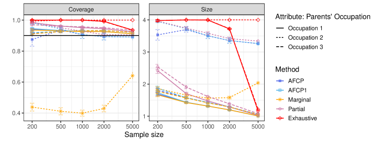
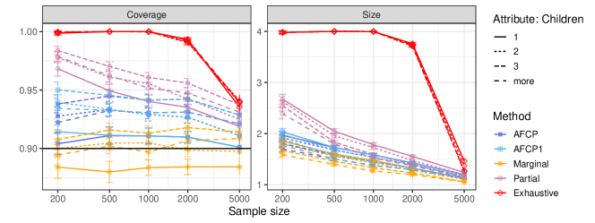
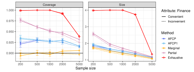
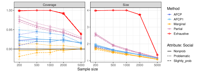

| AFCP | AFCP1 | Marginal | Partial | Exhaustive | |||||||
| Group | Sample size | Coverage | Size | Coverage | Size | Coverage | Size | Coverage | Size | Coverage | Size |
| Occupation 0 | |||||||||||
| Occupation 0 | 200 | 0.940 (0.003) | 1.692 (0.028) | 0.945 (0.003) | 1.731 (0.031) | 0.936 (0.004) | 1.665 (0.029) | 0.983 (0.002) | 2.420 (0.044) | 1.000 (0.000) | 3.980 (0.014) |
| Occupation 0 | 500 | 0.933 (0.002) | 1.433 (0.012) | 0.933 (0.002) | 1.433 (0.012) | 0.931 (0.003) | 1.424 (0.013) | 0.961 (0.002) | 1.703 (0.021) | 1.000 (0.000) | 4.000 (0.000) |
| Occupation 0 | 1000 | 0.927 (0.002) | 1.315 (0.009) | 0.927 (0.002) | 1.315 (0.009) | 0.925 (0.002) | 1.314 (0.009) | 0.951 (0.002) | 1.475 (0.015) | 1.000 (0.000) | 3.996 (0.001) |
| Occupation 0 | 2000 | 0.926 (0.002) | 1.197 (0.007) | 0.926 (0.002) | 1.197 (0.007) | 0.926 (0.002) | 1.196 (0.006) | 0.944 (0.002) | 1.286 (0.008) | 0.992 (0.001) | 3.720 (0.010) |
| Occupation 0 | 5000 | 0.912 (0.002) | 1.010 (0.004) | 0.912 (0.002) | 1.010 (0.004) | 0.912 (0.002) | 1.007 (0.003) | 0.925 (0.002) | 1.028 (0.004) | 0.936 (0.002) | 1.167 (0.009) |
| Occupation 1 | |||||||||||
| Occupation 1 | 200 | 0.875 (0.022) | 3.533 (0.082) | 0.984 (0.006) | 3.952 (0.017) | 0.438 (0.013) | 1.862 (0.031) | 0.988 (0.006) | 3.965 (0.016) | 0.993 (0.005) | 3.980 (0.014) |
| Occupation 1 | 500 | 0.937 (0.009) | 3.699 (0.041) | 0.943 (0.008) | 3.727 (0.034) | 0.411 (0.012) | 1.657 (0.024) | 0.950 (0.006) | 3.742 (0.027) | 1.000 (0.000) | 4.000 (0.000) |
| Occupation 1 | 1000 | 0.906 (0.012) | 3.505 (0.042) | 0.906 (0.012) | 3.505 (0.042) | 0.399 (0.010) | 1.561 (0.020) | 0.928 (0.007) | 3.585 (0.026) | 1.000 (0.000) | 4.000 (0.000) |
| Occupation 1 | 2000 | 0.893 (0.010) | 3.356 (0.041) | 0.893 (0.010) | 3.356 (0.041) | 0.429 (0.011) | 1.579 (0.020) | 0.906 (0.007) | 3.416 (0.027) | 1.000 (0.000) | 4.000 (0.000) |
| Occupation 1 | 5000 | 0.891 (0.010) | 3.263 (0.038) | 0.891 (0.010) | 3.263 (0.038) | 0.641 (0.012) | 2.037 (0.021) | 0.904 (0.006) | 3.341 (0.025) | 1.000 (0.000) | 4.000 (0.000) |
| Occupation 2 | |||||||||||
| Occupation 2 | 200 | 0.913 (0.004) | 1.810 (0.033) | 0.919 (0.004) | 1.868 (0.035) | 0.911 (0.004) | 1.772 (0.029) | 0.970 (0.003) | 2.534 (0.041) | 0.999 (0.001) | 3.980 (0.014) |
| Occupation 2 | 500 | 0.927 (0.003) | 1.577 (0.018) | 0.927 (0.003) | 1.577 (0.018) | 0.926 (0.003) | 1.566 (0.018) | 0.961 (0.002) | 1.906 (0.026) | 1.000 (0.000) | 4.000 (0.000) |
| Occupation 2 | 1000 | 0.932 (0.002) | 1.428 (0.011) | 0.932 (0.002) | 1.428 (0.011) | 0.931 (0.002) | 1.415 (0.011) | 0.956 (0.002) | 1.614 (0.016) | 1.000 (0.000) | 3.998 (0.001) |
| Occupation 2 | 2000 | 0.933 (0.002) | 1.289 (0.007) | 0.933 (0.002) | 1.289 (0.007) | 0.933 (0.002) | 1.285 (0.007) | 0.951 (0.002) | 1.387 (0.009) | 0.991 (0.001) | 3.726 (0.010) |
| Occupation 2 | 5000 | 0.922 (0.002) | 1.056 (0.005) | 0.922 (0.002) | 1.056 (0.005) | 0.921 (0.002) | 1.053 (0.004) | 0.934 (0.002) | 1.082 (0.005) | 0.935 (0.002) | 1.210 (0.009) |
| AFCP | AFCP1 | Marginal | Partial | Exhaustive | |||||||
| Group | Sample size | Coverage | Size | Coverage | Size | Coverage | Size | Coverage | Size | Coverage | Size |
| 1 | |||||||||||
| 1 | 200 | 0.904 (0.004) | 1.966 (0.033) | 0.914 (0.004) | 2.034 (0.034) | 0.884 (0.005) | 1.853 (0.032) | 0.968 (0.003) | 2.673 (0.048) | 0.999 (0.001) | 3.980 (0.014) |
| 1 | 500 | 0.911 (0.004) | 1.728 (0.019) | 0.911 (0.004) | 1.730 (0.019) | 0.880 (0.005) | 1.600 (0.019) | 0.949 (0.003) | 2.047 (0.026) | 1.000 (0.000) | 4.000 (0.000) |
| 1 | 1000 | 0.911 (0.003) | 1.581 (0.014) | 0.911 (0.003) | 1.581 (0.014) | 0.884 (0.003) | 1.475 (0.013) | 0.940 (0.003) | 1.784 (0.018) | 1.000 (0.000) | 3.998 (0.001) |
| 1 | 2000 | 0.910 (0.002) | 1.428 (0.009) | 0.910 (0.002) | 1.428 (0.009) | 0.884 (0.003) | 1.326 (0.009) | 0.935 (0.003) | 1.554 (0.012) | 0.993 (0.001) | 3.758 (0.014) |
| 1 | 5000 | 0.901 (0.003) | 1.198 (0.009) | 0.901 (0.003) | 1.198 (0.009) | 0.884 (0.003) | 1.122 (0.006) | 0.919 (0.003) | 1.238 (0.009) | 0.935 (0.003) | 1.463 (0.016) |
| 2 | |||||||||||
| 2 | 200 | 0.928 (0.004) | 1.917 (0.032) | 0.939 (0.003) | 1.983 (0.033) | 0.900 (0.004) | 1.794 (0.030) | 0.978 (0.002) | 2.629 (0.051) | 0.999 (0.001) | 3.980 (0.014) |
| 2 | 500 | 0.933 (0.003) | 1.679 (0.017) | 0.934 (0.003) | 1.680 (0.017) | 0.905 (0.003) | 1.556 (0.017) | 0.961 (0.002) | 1.957 (0.024) | 1.000 (0.000) | 4.000 (0.000) |
| 2 | 1000 | 0.929 (0.003) | 1.535 (0.012) | 0.929 (0.003) | 1.535 (0.012) | 0.905 (0.003) | 1.427 (0.011) | 0.956 (0.002) | 1.725 (0.018) | 1.000 (0.000) | 3.997 (0.002) |
| 2 | 2000 | 0.927 (0.003) | 1.387 (0.008) | 0.927 (0.003) | 1.387 (0.008) | 0.899 (0.003) | 1.283 (0.007) | 0.942 (0.002) | 1.473 (0.010) | 0.991 (0.001) | 3.739 (0.013) |
| 2 | 5000 | 0.911 (0.003) | 1.175 (0.008) | 0.911 (0.003) | 1.175 (0.008) | 0.898 (0.004) | 1.105 (0.005) | 0.925 (0.003) | 1.198 (0.008) | 0.941 (0.003) | 1.370 (0.012) |
| 3 | |||||||||||
| 3 | 200 | 0.938 (0.004) | 1.806 (0.031) | 0.950 (0.003) | 1.882 (0.032) | 0.908 (0.004) | 1.670 (0.027) | 0.984 (0.002) | 2.544 (0.051) | 1.000 (0.000) | 3.980 (0.014) |
| 3 | 500 | 0.945 (0.002) | 1.579 (0.015) | 0.945 (0.002) | 1.581 (0.015) | 0.916 (0.003) | 1.460 (0.016) | 0.970 (0.002) | 1.834 (0.024) | 1.000 (0.000) | 4.000 (0.000) |
| 3 | 1000 | 0.941 (0.002) | 1.451 (0.011) | 0.941 (0.002) | 1.451 (0.011) | 0.913 (0.003) | 1.332 (0.011) | 0.961 (0.002) | 1.592 (0.015) | 1.000 (0.000) | 3.998 (0.001) |
| 3 | 2000 | 0.942 (0.002) | 1.324 (0.008) | 0.942 (0.002) | 1.324 (0.008) | 0.918 (0.002) | 1.230 (0.007) | 0.956 (0.002) | 1.401 (0.010) | 0.991 (0.001) | 3.713 (0.015) |
| 3 | 5000 | 0.929 (0.003) | 1.128 (0.008) | 0.929 (0.003) | 1.128 (0.008) | 0.914 (0.003) | 1.056 (0.005) | 0.937 (0.002) | 1.142 (0.008) | 0.939 (0.002) | 1.262 (0.012) |
| more | |||||||||||
| more | 200 | 0.922 (0.004) | 1.698 (0.026) | 0.934 (0.004) | 1.772 (0.029) | 0.894 (0.004) | 1.586 (0.025) | 0.979 (0.002) | 2.392 (0.051) | 0.999 (0.000) | 3.980 (0.014) |
| more | 500 | 0.932 (0.003) | 1.502 (0.015) | 0.933 (0.003) | 1.503 (0.015) | 0.902 (0.003) | 1.396 (0.014) | 0.962 (0.003) | 1.795 (0.028) | 1.000 (0.000) | 4.000 (0.000) |
| more | 1000 | 0.931 (0.002) | 1.376 (0.010) | 0.931 (0.002) | 1.376 (0.010) | 0.897 (0.003) | 1.266 (0.010) | 0.952 (0.002) | 1.519 (0.017) | 1.000 (0.000) | 3.996 (0.002) |
| more | 2000 | 0.931 (0.003) | 1.296 (0.008) | 0.931 (0.003) | 1.296 (0.008) | 0.907 (0.003) | 1.197 (0.007) | 0.948 (0.002) | 1.371 (0.009) | 0.993 (0.001) | 3.739 (0.015) |
| more | 5000 | 0.921 (0.003) | 1.121 (0.008) | 0.921 (0.003) | 1.121 (0.008) | 0.909 (0.003) | 1.055 (0.005) | 0.931 (0.003) | 1.139 (0.008) | 0.940 (0.003) | 1.274 (0.013) |
| AFCP | AFCP1 | Marginal | Partial | Exhaustive | |||||||
| Group | Sample size | Coverage | Size | Coverage | Size | Coverage | Size | Coverage | Size | Coverage | Size |
| Convenient | |||||||||||
| Convenient | 200 | 0.921 (0.004) | 1.873 (0.029) | 0.933 (0.003) | 1.946 (0.031) | 0.894 (0.004) | 1.755 (0.028) | 0.976 (0.002) | 2.596 (0.040) | 0.999 (0.001) | 3.980 (0.014) |
| Convenient | 500 | 0.930 (0.002) | 1.665 (0.015) | 0.930 (0.002) | 1.667 (0.015) | 0.901 (0.003) | 1.547 (0.015) | 0.961 (0.002) | 1.961 (0.022) | 1.000 (0.000) | 4.000 (0.000) |
| Convenient | 1000 | 0.927 (0.002) | 1.531 (0.010) | 0.927 (0.002) | 1.531 (0.010) | 0.897 (0.002) | 1.414 (0.009) | 0.951 (0.002) | 1.707 (0.015) | 1.000 (0.000) | 3.997 (0.001) |
| Convenient | 2000 | 0.930 (0.002) | 1.393 (0.008) | 0.930 (0.002) | 1.393 (0.008) | 0.905 (0.002) | 1.293 (0.007) | 0.947 (0.002) | 1.490 (0.009) | 0.992 (0.001) | 3.739 (0.008) |
| Convenient | 5000 | 0.917 (0.002) | 1.165 (0.006) | 0.917 (0.002) | 1.165 (0.006) | 0.906 (0.002) | 1.097 (0.004) | 0.932 (0.002) | 1.194 (0.006) | 0.939 (0.002) | 1.347 (0.010) |
| Inconvenient | |||||||||||
| Inconvenient | 200 | 0.924 (0.004) | 1.821 (0.028) | 0.935 (0.003) | 1.889 (0.029) | 0.899 (0.004) | 1.698 (0.027) | 0.978 (0.002) | 2.521 (0.040) | 0.999 (0.001) | 3.980 (0.014) |
| Inconvenient | 500 | 0.931 (0.002) | 1.582 (0.015) | 0.931 (0.002) | 1.583 (0.015) | 0.901 (0.003) | 1.462 (0.015) | 0.961 (0.002) | 1.857 (0.022) | 1.000 (0.000) | 4.000 (0.000) |
| Inconvenient | 1000 | 0.929 (0.002) | 1.440 (0.010) | 0.929 (0.002) | 1.440 (0.010) | 0.902 (0.003) | 1.336 (0.010) | 0.953 (0.002) | 1.601 (0.015) | 1.000 (0.000) | 3.997 (0.001) |
| Inconvenient | 2000 | 0.925 (0.002) | 1.325 (0.006) | 0.925 (0.002) | 1.325 (0.006) | 0.899 (0.002) | 1.224 (0.006) | 0.943 (0.002) | 1.410 (0.008) | 0.993 (0.001) | 3.736 (0.010) |
| Inconvenient | 5000 | 0.915 (0.002) | 1.146 (0.006) | 0.915 (0.002) | 1.146 (0.006) | 0.897 (0.002) | 1.072 (0.004) | 0.925 (0.002) | 1.166 (0.006) | 0.938 (0.002) | 1.337 (0.010) |
| AFCP | AFCP1 | Marginal | Partial | Exhaustive | |||||||
| Group | Sample size | Coverage | Size | Coverage | Size | Coverage | Size | Coverage | Size | Coverage | Size |
| Nonprob | |||||||||||
| Nonprob | 200 | 0.922 (0.004) | 1.894 (0.031) | 0.933 (0.004) | 1.964 (0.032) | 0.896 (0.004) | 1.775 (0.030) | 0.976 (0.002) | 2.605 (0.041) | 0.999 (0.001) | 3.980 (0.014) |
| Nonprob | 500 | 0.926 (0.003) | 1.655 (0.018) | 0.926 (0.003) | 1.657 (0.017) | 0.897 (0.004) | 1.538 (0.018) | 0.959 (0.002) | 1.943 (0.023) | 1.000 (0.000) | 4.000 (0.000) |
| Nonprob | 1000 | 0.924 (0.003) | 1.509 (0.012) | 0.924 (0.003) | 1.509 (0.012) | 0.899 (0.003) | 1.406 (0.012) | 0.951 (0.002) | 1.694 (0.017) | 1.000 (0.000) | 3.998 (0.001) |
| Nonprob | 2000 | 0.922 (0.002) | 1.360 (0.008) | 0.922 (0.002) | 1.360 (0.008) | 0.896 (0.003) | 1.258 (0.008) | 0.942 (0.002) | 1.456 (0.011) | 0.991 (0.001) | 3.740 (0.012) |
| Nonprob | 5000 | 0.917 (0.003) | 1.164 (0.007) | 0.917 (0.003) | 1.164 (0.007) | 0.901 (0.003) | 1.092 (0.005) | 0.927 (0.002) | 1.186 (0.007) | 0.938 (0.003) | 1.360 (0.013) |
| Problematic | |||||||||||
| Problematic | 200 | 0.937 (0.004) | 1.846 (0.030) | 0.949 (0.004) | 1.916 (0.030) | 0.913 (0.004) | 1.726 (0.028) | 0.984 (0.002) | 2.546 (0.041) | 1.000 (0.000) | 3.980 (0.014) |
| Problematic | 500 | 0.945 (0.002) | 1.626 (0.014) | 0.945 (0.002) | 1.628 (0.014) | 0.913 (0.003) | 1.500 (0.015) | 0.967 (0.002) | 1.892 (0.023) | 1.000 (0.000) | 4.000 (0.000) |
| Problematic | 1000 | 0.941 (0.002) | 1.486 (0.010) | 0.941 (0.002) | 1.486 (0.010) | 0.909 (0.003) | 1.369 (0.009) | 0.958 (0.002) | 1.639 (0.014) | 1.000 (0.000) | 3.996 (0.002) |
| Problematic | 2000 | 0.936 (0.002) | 1.337 (0.008) | 0.936 (0.002) | 1.337 (0.008) | 0.909 (0.003) | 1.238 (0.007) | 0.950 (0.002) | 1.417 (0.009) | 0.993 (0.001) | 3.726 (0.012) |
| Problematic | 5000 | 0.916 (0.003) | 1.135 (0.006) | 0.916 (0.003) | 1.135 (0.006) | 0.903 (0.003) | 1.066 (0.004) | 0.931 (0.002) | 1.160 (0.006) | 0.939 (0.002) | 1.312 (0.010) |
| Slightly_prob | |||||||||||
| Slightly_prob | 200 | 0.909 (0.004) | 1.800 (0.027) | 0.921 (0.004) | 1.871 (0.029) | 0.881 (0.004) | 1.677 (0.026) | 0.971 (0.003) | 2.526 (0.044) | 0.999 (0.001) | 3.980 (0.014) |
| Slightly_prob | 500 | 0.920 (0.003) | 1.590 (0.016) | 0.920 (0.003) | 1.590 (0.016) | 0.891 (0.003) | 1.476 (0.016) | 0.956 (0.002) | 1.893 (0.026) | 1.000 (0.000) | 4.000 (0.000) |
| Slightly_prob | 1000 | 0.919 (0.003) | 1.462 (0.011) | 0.919 (0.003) | 1.462 (0.011) | 0.891 (0.003) | 1.351 (0.011) | 0.947 (0.002) | 1.629 (0.018) | 1.000 (0.000) | 3.997 (0.001) |
| Slightly_prob | 2000 | 0.925 (0.002) | 1.378 (0.008) | 0.925 (0.002) | 1.378 (0.008) | 0.900 (0.003) | 1.282 (0.006) | 0.944 (0.002) | 1.475 (0.009) | 0.993 (0.001) | 3.746 (0.011) |
| Slightly_prob | 5000 | 0.914 (0.002) | 1.167 (0.006) | 0.914 (0.002) | 1.167 (0.006) | 0.900 (0.003) | 1.096 (0.005) | 0.927 (0.002) | 1.193 (0.007) | 0.939 (0.002) | 1.354 (0.011) |
| AFCP | AFCP1 | Marginal | Partial | Exhaustive | |||||||
| Group | Sample size | Coverage | Size | Coverage | Size | Coverage | Size | Coverage | Size | Coverage | Size |
| Not-Recommended | |||||||||||
| Not-Recommended | 200 | 0.961 (0.003) | 1.357 (0.031) | 0.967 (0.003) | 1.419 (0.031) | 0.942 (0.003) | 1.223 (0.029) | 0.990 (0.001) | 1.951 (0.052) | 1.000 (0.000) | 3.980 (0.014) |
| Not-Recommended | 500 | 0.950 (0.002) | 1.136 (0.008) | 0.950 (0.002) | 1.139 (0.008) | 0.931 (0.003) | 1.006 (0.007) | 0.971 (0.002) | 1.228 (0.013) | 1.000 (0.000) | 4.000 (0.000) |
| Not-Recommended | 1000 | 0.942 (0.002) | 1.086 (0.007) | 0.942 (0.002) | 1.086 (0.007) | 0.925 (0.003) | 0.985 (0.005) | 0.958 (0.002) | 1.130 (0.008) | 1.000 (0.000) | 3.995 (0.002) |
| Not-Recommended | 2000 | 0.935 (0.002) | 1.051 (0.005) | 0.935 (0.002) | 1.051 (0.005) | 0.922 (0.002) | 0.966 (0.003) | 0.948 (0.002) | 1.072 (0.005) | 0.994 (0.001) | 3.697 (0.013) |
| Not-Recommended | 5000 | 0.927 (0.002) | 1.033 (0.005) | 0.927 (0.002) | 1.033 (0.005) | 0.915 (0.002) | 0.969 (0.003) | 0.937 (0.002) | 1.048 (0.005) | 0.940 (0.002) | 1.164 (0.009) |
| Priority | |||||||||||
| Priority | 200 | 0.938 (0.004) | 2.249 (0.038) | 0.948 (0.003) | 2.326 (0.039) | 0.909 (0.004) | 2.145 (0.038) | 0.979 (0.002) | 2.987 (0.044) | 1.000 (0.000) | 3.980 (0.014) |
| Priority | 500 | 0.946 (0.002) | 1.866 (0.026) | 0.946 (0.002) | 1.867 (0.026) | 0.912 (0.003) | 1.751 (0.026) | 0.967 (0.002) | 2.229 (0.036) | 1.000 (0.000) | 4.000 (0.000) |
| Priority | 1000 | 0.945 (0.002) | 1.601 (0.015) | 0.945 (0.002) | 1.601 (0.015) | 0.907 (0.003) | 1.484 (0.016) | 0.960 (0.002) | 1.788 (0.021) | 1.000 (0.000) | 3.998 (0.001) |
| Priority | 2000 | 0.933 (0.002) | 1.384 (0.010) | 0.933 (0.002) | 1.384 (0.010) | 0.901 (0.002) | 1.278 (0.009) | 0.948 (0.002) | 1.476 (0.013) | 0.991 (0.001) | 3.734 (0.011) |
| Priority | 5000 | 0.908 (0.003) | 1.140 (0.008) | 0.908 (0.003) | 1.140 (0.008) | 0.896 (0.003) | 1.073 (0.005) | 0.924 (0.003) | 1.167 (0.007) | 0.937 (0.002) | 1.330 (0.010) |
| Recommended | |||||||||||
| Recommended | 200 | 0.871 (0.006) | 1.933 (0.031) | 0.888 (0.006) | 2.006 (0.033) | 0.839 (0.006) | 1.809 (0.028) | 0.962 (0.004) | 2.736 (0.043) | 0.998 (0.001) | 3.980 (0.014) |
| Recommended | 500 | 0.895 (0.004) | 1.869 (0.020) | 0.896 (0.004) | 1.870 (0.020) | 0.859 (0.004) | 1.757 (0.020) | 0.945 (0.003) | 2.273 (0.029) | 1.000 (0.000) | 4.000 (0.000) |
| Recommended | 1000 | 0.898 (0.003) | 1.775 (0.014) | 0.898 (0.003) | 1.775 (0.014) | 0.867 (0.003) | 1.662 (0.014) | 0.938 (0.002) | 2.053 (0.023) | 1.000 (0.000) | 3.998 (0.001) |
| Recommended | 2000 | 0.914 (0.003) | 1.646 (0.011) | 0.914 (0.003) | 1.646 (0.011) | 0.883 (0.003) | 1.539 (0.010) | 0.940 (0.002) | 1.807 (0.013) | 0.991 (0.001) | 3.780 (0.010) |
| Recommended | 5000 | 0.912 (0.003) | 1.293 (0.010) | 0.912 (0.003) | 1.293 (0.010) | 0.894 (0.002) | 1.213 (0.007) | 0.924 (0.002) | 1.324 (0.010) | 0.939 (0.002) | 1.532 (0.014) |
Next, we provide numerical experimental results comparing AFCP with the label-conditional adaptive equalized coverage (see Equation (A14)) with other benchmark methods.

| AFCP | AFCP1 | Marginal | Partial | Exhaustive | ||||||
| Sample size | Coverage | Size | Coverage | Size | Coverage | Size | Coverage | Size | Coverage | Size |
| 200 | 0.925 (0.003) | 2.745 (0.029) | 0.962 (0.002) | 3.841 (0.017) | 0.919 (0.003) | 2.575 (0.023) | 0.996 (0.001) | 3.970 (0.014) | 0.999 (0.001) | 3.980 (0.014) |
| 500 | 0.924 (0.002) | 2.934 (0.034) | 0.944 (0.002) | 3.670 (0.008) | 0.910 (0.002) | 2.214 (0.019) | 0.978 (0.001) | 3.811 (0.007) | 1.000 (0.000) | 4.000 (0.000) |
| 1000 | 0.922 (0.002) | 2.994 (0.029) | 0.933 (0.002) | 3.505 (0.006) | 0.905 (0.002) | 1.954 (0.015) | 0.966 (0.001) | 3.649 (0.006) | 1.000 (0.000) | 4.000 (0.000) |
| 2000 | 0.923 (0.001) | 2.937 (0.025) | 0.927 (0.001) | 3.352 (0.010) | 0.904 (0.001) | 1.712 (0.019) | 0.954 (0.001) | 3.495 (0.007) | 0.997 (0.000) | 3.996 (0.000) |
| 5000 | 0.913 (0.001) | 1.893 (0.022) | 0.915 (0.001) | 2.426 (0.022) | 0.902 (0.001) | 1.127 (0.005) | 0.935 (0.001) | 2.593 (0.019) | 0.956 (0.001) | 3.872 (0.002) |
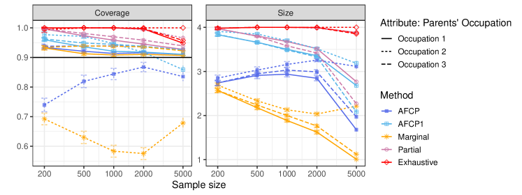
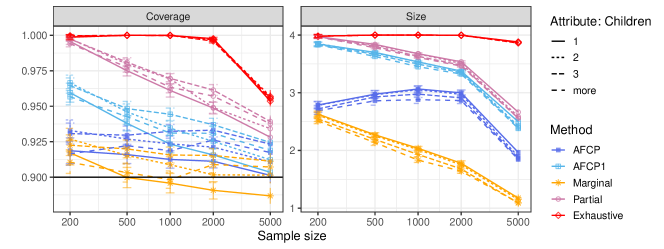
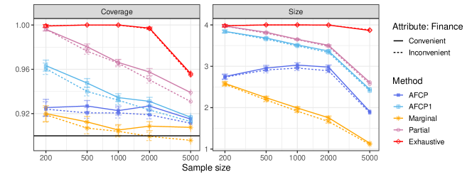
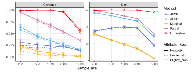

| AFCP | AFCP1 | Marginal | Partial | Exhaustive | |||||||
| Group | Sample size | Coverage | Size | Coverage | Size | Coverage | Size | Coverage | Size | Coverage | Size |
| Occupation 0 | |||||||||||
| Occupation 0 | 200 | 0.934 (0.004) | 2.740 (0.029) | 0.960 (0.003) | 3.831 (0.018) | 0.932 (0.004) | 2.569 (0.024) | 0.996 (0.001) | 3.967 (0.014) | 1.000 (0.000) | 3.980 (0.014) |
| Occupation 0 | 500 | 0.921 (0.003) | 2.911 (0.036) | 0.936 (0.002) | 3.662 (0.011) | 0.913 (0.003) | 2.177 (0.022) | 0.973 (0.002) | 3.803 (0.008) | 1.000 (0.000) | 4.000 (0.000) |
| Occupation 0 | 1000 | 0.914 (0.002) | 2.937 (0.030) | 0.921 (0.002) | 3.502 (0.009) | 0.908 (0.003) | 1.888 (0.017) | 0.958 (0.002) | 3.677 (0.007) | 1.000 (0.000) | 4.000 (0.000) |
| Occupation 0 | 2000 | 0.916 (0.002) | 2.845 (0.028) | 0.918 (0.002) | 3.356 (0.012) | 0.910 (0.002) | 1.624 (0.022) | 0.945 (0.002) | 3.518 (0.008) | 0.996 (0.000) | 3.995 (0.000) |
| Occupation 0 | 5000 | 0.910 (0.002) | 1.679 (0.021) | 0.911 (0.002) | 2.681 (0.019) | 0.907 (0.002) | 1.009 (0.004) | 0.927 (0.002) | 2.768 (0.016) | 0.948 (0.002) | 3.877 (0.003) |
| Occupation 1 | |||||||||||
| Occupation 1 | 200 | 0.739 (0.012) | 2.850 (0.034) | 0.977 (0.005) | 3.907 (0.016) | 0.692 (0.010) | 2.689 (0.026) | 0.993 (0.005) | 3.980 (0.014) | 0.993 (0.005) | 3.980 (0.014) |
| Occupation 1 | 500 | 0.819 (0.011) | 3.031 (0.036) | 0.971 (0.003) | 3.848 (0.011) | 0.630 (0.011) | 2.334 (0.022) | 1.000 (0.000) | 4.000 (0.000) | 1.000 (0.000) | 4.000 (0.000) |
| Occupation 1 | 1000 | 0.844 (0.010) | 3.159 (0.032) | 0.947 (0.005) | 3.699 (0.015) | 0.583 (0.010) | 2.130 (0.019) | 1.000 (0.000) | 3.999 (0.001) | 1.000 (0.000) | 4.000 (0.000) |
| Occupation 1 | 2000 | 0.868 (0.008) | 3.257 (0.019) | 0.917 (0.006) | 3.516 (0.016) | 0.575 (0.010) | 2.034 (0.019) | 0.994 (0.002) | 3.982 (0.004) | 1.000 (0.000) | 4.000 (0.000) |
| Occupation 1 | 5000 | 0.835 (0.008) | 3.114 (0.027) | 0.859 (0.007) | 3.185 (0.025) | 0.679 (0.009) | 2.213 (0.019) | 0.966 (0.004) | 3.885 (0.010) | 1.000 (0.000) | 4.000 (0.000) |
| Occupation 2 | |||||||||||
| Occupation 2 | 200 | 0.938 (0.004) | 2.739 (0.031) | 0.962 (0.003) | 3.841 (0.018) | 0.934 (0.003) | 2.569 (0.024) | 0.996 (0.001) | 3.973 (0.014) | 0.999 (0.001) | 3.980 (0.014) |
| Occupation 2 | 500 | 0.938 (0.002) | 2.947 (0.033) | 0.949 (0.002) | 3.658 (0.012) | 0.939 (0.002) | 2.237 (0.017) | 0.981 (0.001) | 3.797 (0.011) | 1.000 (0.000) | 4.000 (0.000) |
| Occupation 2 | 1000 | 0.939 (0.002) | 3.030 (0.028) | 0.944 (0.002) | 3.486 (0.007) | 0.938 (0.002) | 2.000 (0.015) | 0.970 (0.002) | 3.581 (0.007) | 1.000 (0.000) | 4.000 (0.000) |
| Occupation 2 | 2000 | 0.936 (0.002) | 2.990 (0.026) | 0.938 (0.002) | 3.329 (0.010) | 0.936 (0.002) | 1.763 (0.019) | 0.958 (0.002) | 3.417 (0.008) | 0.997 (0.000) | 3.996 (0.000) |
| Occupation 2 | 5000 | 0.925 (0.002) | 1.971 (0.029) | 0.926 (0.002) | 2.083 (0.030) | 0.922 (0.002) | 1.123 (0.007) | 0.939 (0.002) | 2.269 (0.028) | 0.958 (0.002) | 3.852 (0.003) |
| AFCP | AFCP1 | Marginal | Partial | Exhaustive | |||||||
| Group | Sample size | Coverage | Size | Coverage | Size | Coverage | Size | Coverage | Size | Coverage | Size |
| 1 | |||||||||||
| 1 | 200 | 0.919 (0.005) | 2.788 (0.031) | 0.960 (0.003) | 3.844 (0.017) | 0.917 (0.004) | 2.631 (0.026) | 0.996 (0.001) | 3.972 (0.014) | 0.999 (0.001) | 3.980 (0.014) |
| 1 | 500 | 0.916 (0.003) | 2.975 (0.033) | 0.938 (0.003) | 3.699 (0.010) | 0.900 (0.004) | 2.271 (0.018) | 0.975 (0.002) | 3.838 (0.010) | 1.000 (0.000) | 4.000 (0.000) |
| 1 | 1000 | 0.912 (0.003) | 3.066 (0.028) | 0.923 (0.003) | 3.534 (0.008) | 0.896 (0.003) | 2.038 (0.016) | 0.961 (0.002) | 3.677 (0.008) | 1.000 (0.000) | 4.000 (0.000) |
| 1 | 2000 | 0.911 (0.002) | 2.998 (0.026) | 0.916 (0.002) | 3.375 (0.012) | 0.891 (0.003) | 1.779 (0.021) | 0.949 (0.002) | 3.536 (0.009) | 0.998 (0.000) | 3.997 (0.001) |
| 1 | 5000 | 0.901 (0.003) | 1.967 (0.023) | 0.903 (0.003) | 2.498 (0.024) | 0.887 (0.003) | 1.176 (0.007) | 0.928 (0.002) | 2.664 (0.020) | 0.954 (0.002) | 3.880 (0.003) |
| 2 | |||||||||||
| 2 | 200 | 0.933 (0.004) | 2.782 (0.030) | 0.967 (0.003) | 3.851 (0.017) | 0.927 (0.004) | 2.613 (0.024) | 0.998 (0.001) | 3.972 (0.014) | 0.999 (0.001) | 3.980 (0.014) |
| 2 | 500 | 0.927 (0.003) | 2.966 (0.034) | 0.946 (0.003) | 3.686 (0.010) | 0.915 (0.003) | 2.251 (0.020) | 0.980 (0.002) | 3.824 (0.008) | 1.000 (0.000) | 4.000 (0.000) |
| 2 | 1000 | 0.923 (0.003) | 3.052 (0.029) | 0.935 (0.002) | 3.536 (0.007) | 0.909 (0.003) | 2.015 (0.014) | 0.969 (0.002) | 3.675 (0.007) | 1.000 (0.000) | 4.000 (0.000) |
| 2 | 2000 | 0.921 (0.003) | 2.972 (0.026) | 0.925 (0.003) | 3.364 (0.011) | 0.902 (0.003) | 1.750 (0.020) | 0.949 (0.002) | 3.506 (0.007) | 0.997 (0.001) | 3.996 (0.001) |
| 2 | 5000 | 0.911 (0.003) | 1.895 (0.024) | 0.912 (0.003) | 2.425 (0.023) | 0.901 (0.003) | 1.150 (0.007) | 0.934 (0.002) | 2.589 (0.022) | 0.957 (0.002) | 3.876 (0.004) |
| 3 | |||||||||||
| 3 | 200 | 0.931 (0.004) | 2.721 (0.030) | 0.965 (0.003) | 3.837 (0.017) | 0.923 (0.004) | 2.547 (0.024) | 0.997 (0.001) | 3.971 (0.015) | 1.000 (0.000) | 3.980 (0.014) |
| 3 | 500 | 0.930 (0.003) | 2.928 (0.035) | 0.948 (0.003) | 3.664 (0.010) | 0.920 (0.003) | 2.191 (0.020) | 0.981 (0.002) | 3.803 (0.009) | 1.000 (0.000) | 4.000 (0.000) |
| 3 | 1000 | 0.932 (0.002) | 2.976 (0.029) | 0.944 (0.002) | 3.497 (0.008) | 0.916 (0.003) | 1.931 (0.019) | 0.970 (0.002) | 3.632 (0.007) | 1.000 (0.000) | 4.000 (0.000) |
| 3 | 2000 | 0.933 (0.002) | 2.911 (0.027) | 0.937 (0.002) | 3.347 (0.011) | 0.915 (0.002) | 1.680 (0.021) | 0.961 (0.002) | 3.477 (0.009) | 0.996 (0.001) | 3.995 (0.001) |
| 3 | 5000 | 0.923 (0.002) | 1.865 (0.024) | 0.924 (0.002) | 2.400 (0.023) | 0.911 (0.003) | 1.090 (0.007) | 0.939 (0.002) | 2.559 (0.021) | 0.955 (0.002) | 3.860 (0.004) |
| more | |||||||||||
| more | 200 | 0.916 (0.004) | 2.688 (0.031) | 0.957 (0.003) | 3.830 (0.017) | 0.910 (0.004) | 2.509 (0.023) | 0.994 (0.001) | 3.967 (0.014) | 0.999 (0.000) | 3.980 (0.014) |
| more | 500 | 0.922 (0.003) | 2.860 (0.038) | 0.943 (0.003) | 3.629 (0.010) | 0.903 (0.003) | 2.137 (0.024) | 0.978 (0.002) | 3.779 (0.009) | 1.000 (0.000) | 4.000 (0.000) |
| more | 1000 | 0.919 (0.003) | 2.880 (0.033) | 0.931 (0.003) | 3.451 (0.009) | 0.898 (0.003) | 1.833 (0.020) | 0.963 (0.002) | 3.611 (0.008) | 1.000 (0.000) | 4.000 (0.000) |
| more | 2000 | 0.926 (0.003) | 2.865 (0.026) | 0.931 (0.003) | 3.324 (0.012) | 0.909 (0.003) | 1.641 (0.019) | 0.957 (0.002) | 3.461 (0.009) | 0.997 (0.001) | 3.996 (0.001) |
| more | 5000 | 0.917 (0.003) | 1.846 (0.024) | 0.919 (0.003) | 2.382 (0.023) | 0.907 (0.003) | 1.093 (0.006) | 0.938 (0.002) | 2.559 (0.021) | 0.956 (0.002) | 3.872 (0.003) |
| AFCP | AFCP1 | Marginal | Partial | Exhaustive | |||||||
| Group | Sample size | Coverage | Size | Coverage | Size | Coverage | Size | Coverage | Size | Coverage | Size |
| Convenient | |||||||||||
| Convenient | 200 | 0.925 (0.004) | 2.753 (0.030) | 0.963 (0.002) | 3.843 (0.017) | 0.920 (0.004) | 2.587 (0.024) | 0.996 (0.001) | 3.972 (0.014) | 0.999 (0.001) | 3.980 (0.014) |
| Convenient | 500 | 0.927 (0.002) | 2.957 (0.033) | 0.948 (0.002) | 3.684 (0.009) | 0.913 (0.002) | 2.240 (0.018) | 0.980 (0.001) | 3.822 (0.008) | 1.000 (0.000) | 4.000 (0.000) |
| Convenient | 1000 | 0.923 (0.002) | 3.029 (0.027) | 0.934 (0.002) | 3.517 (0.007) | 0.905 (0.002) | 1.993 (0.015) | 0.966 (0.001) | 3.653 (0.006) | 1.000 (0.000) | 4.000 (0.000) |
| Convenient | 2000 | 0.927 (0.002) | 2.980 (0.026) | 0.931 (0.002) | 3.369 (0.010) | 0.909 (0.002) | 1.757 (0.020) | 0.958 (0.002) | 3.508 (0.008) | 0.997 (0.000) | 3.996 (0.000) |
| Convenient | 5000 | 0.915 (0.002) | 1.908 (0.022) | 0.917 (0.002) | 2.445 (0.022) | 0.908 (0.002) | 1.143 (0.006) | 0.939 (0.002) | 2.614 (0.019) | 0.956 (0.002) | 3.866 (0.003) |
| Inconvenient | |||||||||||
| Inconvenient | 200 | 0.924 (0.003) | 2.737 (0.029) | 0.961 (0.003) | 3.839 (0.017) | 0.919 (0.003) | 2.564 (0.023) | 0.996 (0.001) | 3.969 (0.014) | 0.999 (0.001) | 3.980 (0.014) |
| Inconvenient | 500 | 0.921 (0.002) | 2.911 (0.035) | 0.940 (0.002) | 3.656 (0.009) | 0.907 (0.003) | 2.188 (0.021) | 0.976 (0.001) | 3.800 (0.008) | 1.000 (0.000) | 4.000 (0.000) |
| Inconvenient | 1000 | 0.921 (0.002) | 2.957 (0.030) | 0.932 (0.002) | 3.492 (0.007) | 0.904 (0.003) | 1.915 (0.016) | 0.966 (0.002) | 3.644 (0.007) | 1.000 (0.000) | 4.000 (0.000) |
| Inconvenient | 2000 | 0.919 (0.002) | 2.892 (0.026) | 0.923 (0.002) | 3.335 (0.011) | 0.899 (0.002) | 1.666 (0.020) | 0.950 (0.001) | 3.483 (0.008) | 0.997 (0.000) | 3.996 (0.000) |
| Inconvenient | 5000 | 0.911 (0.002) | 1.879 (0.023) | 0.913 (0.002) | 2.409 (0.023) | 0.896 (0.002) | 1.112 (0.005) | 0.931 (0.002) | 2.573 (0.020) | 0.955 (0.001) | 3.878 (0.002) |
| AFCP | AFCP1 | Marginal | Partial | Exhaustive | |||||||
| Group | Sample size | Coverage | Size | Coverage | Size | Coverage | Size | Coverage | Size | Coverage | Size |
| Nonprob | |||||||||||
| Nonprob | 200 | 0.931 (0.004) | 2.768 (0.031) | 0.964 (0.003) | 3.846 (0.017) | 0.924 (0.004) | 2.601 (0.025) | 0.996 (0.001) | 3.971 (0.014) | 0.999 (0.001) | 3.980 (0.014) |
| Nonprob | 500 | 0.926 (0.003) | 2.939 (0.035) | 0.945 (0.003) | 3.674 (0.009) | 0.912 (0.003) | 2.228 (0.020) | 0.979 (0.001) | 3.815 (0.008) | 1.000 (0.000) | 4.000 (0.000) |
| Nonprob | 1000 | 0.924 (0.003) | 3.016 (0.029) | 0.935 (0.002) | 3.515 (0.008) | 0.909 (0.003) | 1.980 (0.016) | 0.968 (0.002) | 3.658 (0.007) | 1.000 (0.000) | 4.000 (0.000) |
| Nonprob | 2000 | 0.921 (0.002) | 2.934 (0.026) | 0.926 (0.002) | 3.355 (0.011) | 0.903 (0.002) | 1.711 (0.021) | 0.954 (0.002) | 3.501 (0.008) | 0.996 (0.001) | 3.996 (0.001) |
| Nonprob | 5000 | 0.915 (0.002) | 1.904 (0.024) | 0.916 (0.002) | 2.437 (0.023) | 0.900 (0.002) | 1.137 (0.007) | 0.934 (0.002) | 2.585 (0.021) | 0.957 (0.002) | 3.875 (0.003) |
| Problematic | |||||||||||
| Problematic | 200 | 0.924 (0.004) | 2.742 (0.030) | 0.963 (0.003) | 3.843 (0.017) | 0.922 (0.004) | 2.573 (0.023) | 0.997 (0.001) | 3.972 (0.014) | 1.000 (0.000) | 3.980 (0.014) |
| Problematic | 500 | 0.923 (0.003) | 2.941 (0.034) | 0.944 (0.002) | 3.674 (0.009) | 0.911 (0.003) | 2.213 (0.019) | 0.978 (0.002) | 3.810 (0.007) | 1.000 (0.000) | 4.000 (0.000) |
| Problematic | 1000 | 0.923 (0.002) | 2.999 (0.029) | 0.935 (0.002) | 3.508 (0.007) | 0.904 (0.003) | 1.954 (0.016) | 0.963 (0.002) | 3.644 (0.007) | 1.000 (0.000) | 4.000 (0.000) |
| Problematic | 2000 | 0.924 (0.002) | 2.914 (0.026) | 0.929 (0.002) | 3.355 (0.011) | 0.904 (0.003) | 1.683 (0.021) | 0.953 (0.002) | 3.486 (0.008) | 0.997 (0.001) | 3.996 (0.001) |
| Problematic | 5000 | 0.912 (0.002) | 1.863 (0.022) | 0.914 (0.002) | 2.394 (0.022) | 0.903 (0.002) | 1.106 (0.005) | 0.935 (0.002) | 2.588 (0.020) | 0.952 (0.002) | 3.871 (0.003) |
| Slightly_prob | |||||||||||
| Slightly_prob | 200 | 0.918 (0.004) | 2.722 (0.029) | 0.958 (0.003) | 3.831 (0.017) | 0.913 (0.004) | 2.550 (0.022) | 0.996 (0.001) | 3.968 (0.014) | 0.999 (0.001) | 3.980 (0.014) |
| Slightly_prob | 500 | 0.921 (0.003) | 2.921 (0.034) | 0.943 (0.002) | 3.662 (0.009) | 0.906 (0.003) | 2.201 (0.020) | 0.978 (0.002) | 3.809 (0.009) | 1.000 (0.000) | 4.000 (0.000) |
| Slightly_prob | 1000 | 0.919 (0.002) | 2.966 (0.030) | 0.931 (0.002) | 3.492 (0.007) | 0.902 (0.002) | 1.929 (0.017) | 0.966 (0.001) | 3.646 (0.007) | 1.000 (0.000) | 4.000 (0.000) |
| Slightly_prob | 2000 | 0.923 (0.002) | 2.963 (0.025) | 0.927 (0.002) | 3.347 (0.012) | 0.905 (0.002) | 1.743 (0.019) | 0.954 (0.002) | 3.498 (0.008) | 0.998 (0.000) | 3.997 (0.000) |
| Slightly_prob | 5000 | 0.913 (0.002) | 1.912 (0.023) | 0.914 (0.002) | 2.448 (0.023) | 0.902 (0.002) | 1.139 (0.006) | 0.935 (0.002) | 2.605 (0.019) | 0.958 (0.002) | 3.871 (0.004) |
| AFCP | AFCP1 | Marginal | Partial | Exhaustive | |||||||
| Group | Sample size | Coverage | Size | Coverage | Size | Coverage | Size | Coverage | Size | Coverage | Size |
| Not-Recommended | |||||||||||
| Not-Recommended | 200 | 0.937 (0.005) | 2.279 (0.038) | 0.947 (0.005) | 3.868 (0.020) | 0.936 (0.005) | 2.193 (0.028) | 0.995 (0.001) | 3.975 (0.014) | 1.000 (0.000) | 3.980 (0.014) |
| Not-Recommended | 500 | 0.929 (0.004) | 2.576 (0.071) | 0.938 (0.003) | 3.915 (0.005) | 0.924 (0.004) | 1.771 (0.033) | 0.981 (0.002) | 3.981 (0.002) | 1.000 (0.000) | 4.000 (0.000) |
| Not-Recommended | 1000 | 0.928 (0.003) | 2.864 (0.069) | 0.936 (0.002) | 3.919 (0.010) | 0.917 (0.003) | 1.504 (0.031) | 0.968 (0.002) | 3.968 (0.002) | 1.000 (0.000) | 4.000 (0.000) |
| Not-Recommended | 2000 | 0.932 (0.002) | 3.129 (0.054) | 0.936 (0.002) | 3.876 (0.018) | 0.921 (0.003) | 1.341 (0.027) | 0.956 (0.002) | 3.956 (0.002) | 0.994 (0.001) | 3.994 (0.001) |
| Not-Recommended | 5000 | 0.914 (0.002) | 2.940 (0.046) | 0.915 (0.002) | 3.541 (0.043) | 0.901 (0.003) | 0.973 (0.005) | 0.929 (0.002) | 3.737 (0.027) | 0.939 (0.002) | 3.939 (0.002) |
| Priority | |||||||||||
| Priority | 200 | 0.931 (0.004) | 3.055 (0.038) | 0.973 (0.002) | 3.833 (0.018) | 0.925 (0.004) | 2.922 (0.032) | 0.997 (0.001) | 3.966 (0.014) | 1.000 (0.000) | 3.980 (0.014) |
| Priority | 500 | 0.928 (0.003) | 2.989 (0.048) | 0.948 (0.002) | 3.511 (0.015) | 0.914 (0.003) | 2.470 (0.022) | 0.980 (0.002) | 3.699 (0.012) | 1.000 (0.000) | 4.000 (0.000) |
| Priority | 1000 | 0.927 (0.003) | 2.946 (0.035) | 0.939 (0.002) | 3.287 (0.009) | 0.907 (0.003) | 2.142 (0.018) | 0.967 (0.002) | 3.439 (0.009) | 1.000 (0.000) | 4.000 (0.000) |
| Priority | 2000 | 0.916 (0.003) | 2.709 (0.024) | 0.922 (0.003) | 3.069 (0.013) | 0.894 (0.003) | 1.781 (0.023) | 0.952 (0.002) | 3.209 (0.012) | 0.998 (0.000) | 3.996 (0.001) |
| Priority | 5000 | 0.910 (0.002) | 1.263 (0.026) | 0.913 (0.002) | 1.765 (0.027) | 0.898 (0.002) | 1.085 (0.005) | 0.934 (0.002) | 1.879 (0.028) | 0.960 (0.002) | 3.833 (0.004) |
| Recommended | |||||||||||
| Recommended | 200 | 0.906 (0.005) | 2.899 (0.043) | 0.965 (0.003) | 3.820 (0.020) | 0.897 (0.005) | 2.607 (0.021) | 0.996 (0.002) | 3.970 (0.014) | 0.998 (0.001) | 3.980 (0.014) |
| Recommended | 500 | 0.914 (0.003) | 3.234 (0.042) | 0.945 (0.003) | 3.582 (0.014) | 0.891 (0.003) | 2.403 (0.013) | 0.975 (0.002) | 3.754 (0.011) | 1.000 (0.000) | 4.000 (0.000) |
| Recommended | 1000 | 0.911 (0.003) | 3.174 (0.025) | 0.925 (0.003) | 3.302 (0.011) | 0.890 (0.003) | 2.224 (0.011) | 0.963 (0.002) | 3.534 (0.010) | 1.000 (0.000) | 4.000 (0.000) |
| Recommended | 2000 | 0.920 (0.002) | 2.969 (0.020) | 0.924 (0.002) | 3.106 (0.016) | 0.897 (0.002) | 2.024 (0.015) | 0.954 (0.002) | 3.316 (0.015) | 0.999 (0.000) | 3.998 (0.000) |
| Recommended | 5000 | 0.916 (0.002) | 1.472 (0.025) | 0.916 (0.002) | 1.969 (0.025) | 0.907 (0.002) | 1.325 (0.010) | 0.943 (0.002) | 2.164 (0.025) | 0.968 (0.001) | 3.845 (0.003) |
A7.2 AFCP for Outlier Detection
A7.2.1 Setup and Benchmarks
This section demonstrates the empirical performance of our AFCP extension for outlier detection. Firstly, we focus on the implementation described in Algorithm A7, which selects at most one sensitive attribute. Similar to the multi-class classification cases, Our method is compared with three existing approaches, which utilize the same data, ML model, and conformity scores but compute conformal p-values with different guarantees. The first is the marginal benchmark, which constructs conformal p-value guaranteeing by applying Algorithm A2 without protected attributes. The second is the exhaustive equalized benchmark, which evaluates conformal p-values guaranteeing by applying Algorithm A2 with all sensitive attributes simultaneously protected. The third is a partial equalized benchmark that separately applies Algorithm A2 with each possible protected attribute , and then takes the maximum of all such p values. This is an intuitive approach that can be easily verified to provide a coverage guarantee .
In addition, similar to the multiclass classification experiments, we consider AFCP1 - the AFCP implementation that always selects the most critical protected attribute without conducting the significance test.
For all methods considered, the outlier detection model is based on a three-layer neural network, and the outputs from each layer are batch-normalized. The Adam optimizer and the BCEWithLogitsLoss loss function are used in the training process, with a learning rate set at 0.0001. The loss values demonstrate convergence after 100 epochs of training. For all methods, the miscoverage target level is set at . Note that the training and testing data contain both inliers and outliers, while the calibration data only contains inliers.
We assess the performance of the methods based on the False Positive Rate (FPR) and the True Positive Rate (TPR). Ideally, the objective is to achieve a higher conditional FPR for groups experiencing unfairness, thereby maintaining the average FPR below the target threshold of 0.1 while simultaneously achieving a higher TPR. The results presented are averaged over 500 independent test points and 30 experiments.
A7.2.2 Synthetic Data
We employ the same data settings as in the multi-class classification example, designating Color as the sensitive attribute associated with the Blue group, which suffers from undercoverage. While Age Group and Region are also sensitive attributes, they are not subject to biases in this context. The outcome labels have two possible values: if the unit is properly treated and otherwise. In our experiment, we treat as an outlier and as an inlier, with the data generation process described as:
| (A28) |
Figure A19 and Table A21 illustrate the performance of conformal p-values generated by various methods on synthetic data, showcasing how performance varies with the number of samples in training and calibration datasets. Figures A20–A21 and Tables A22–A24 separately evaluate the False Positive Rate (FPR) and True Positive Rate (TPR) for each protected attribute. Additionally, Figure A23 explores how the severity of bias affecting groups impacts the selection frequency of our method at various levels. The severity of bias is controlled by the varying percentage of Blue samples, with higher levels indicating less samples and more significant biases in the Blue group.

| AFCP | AFCP1 | Marginal | Partial | Exhaustive | ||||||
| Sample Size | FPR | TPR | FPR | TPR | FPR | TPR | FPR | TPR | FPR | TPR |
| 200 | 0.094 (0.007) | 0.642 (0.025) | 0.069 (0.006) | 0.544 (0.033) | 0.102 (0.008) | 0.649 (0.027) | 0.018 (0.003) | 0.221 (0.023) | 0.000 (0.000) | 0.000 (0.000) |
| 500 | 0.079 (0.005) | 0.706 (0.018) | 0.078 (0.005) | 0.703 (0.018) | 0.085 (0.005) | 0.696 (0.017) | 0.037 (0.003) | 0.519 (0.024) | 0.010 (0.002) | 0.066 (0.006) |
| 1000 | 0.089 (0.005) | 0.780 (0.008) | 0.088 (0.005) | 0.780 (0.008) | 0.096 (0.005) | 0.770 (0.010) | 0.046 (0.003) | 0.664 (0.014) | 0.052 (0.003) | 0.521 (0.011) |
| 2000 | 0.097 (0.005) | 0.804 (0.006) | 0.097 (0.005) | 0.804 (0.006) | 0.101 (0.004) | 0.800 (0.006) | 0.056 (0.004) | 0.720 (0.010) | 0.071 (0.004) | 0.728 (0.008) |
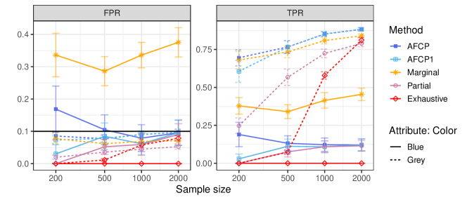
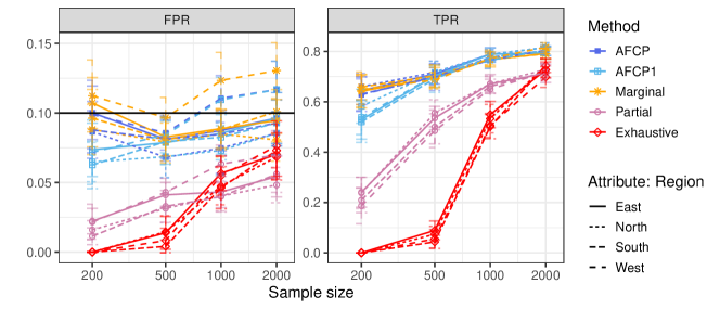
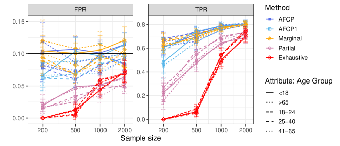
| AFCP | AFCP1 | Marginal | Partial | Exhaustive | |||||||
| Group | Sample Size | FPR | TPR | FPR | TPR | FPR | TPR | FPR | TPR | FPR | TPR |
| Grey | |||||||||||
| Grey | 200 | 0.085 (0.006) | 0.695 (0.027) | 0.073 (0.007) | 0.606 (0.036) | 0.077 (0.007) | 0.680 (0.029) | 0.020 (0.003) | 0.247 (0.026) | 0.000 (0.000) | 0.000 (0.000) |
| Grey | 500 | 0.077 (0.005) | 0.767 (0.021) | 0.078 (0.006) | 0.766 (0.021) | 0.062 (0.006) | 0.734 (0.019) | 0.036 (0.003) | 0.567 (0.027) | 0.011 (0.002) | 0.074 (0.007) |
| Grey | 1000 | 0.090 (0.005) | 0.852 (0.008) | 0.090 (0.005) | 0.853 (0.008) | 0.069 (0.004) | 0.809 (0.011) | 0.045 (0.003) | 0.725 (0.014) | 0.058 (0.004) | 0.579 (0.012) |
| Grey | 2000 | 0.097 (0.005) | 0.883 (0.005) | 0.097 (0.005) | 0.883 (0.005) | 0.071 (0.004) | 0.840 (0.006) | 0.052 (0.004) | 0.789 (0.011) | 0.079 (0.004) | 0.812 (0.009) |
| Blue | |||||||||||
| Blue | 200 | 0.169 (0.036) | 0.190 (0.040) | 0.030 (0.014) | 0.029 (0.016) | 0.336 (0.034) | 0.378 (0.027) | 0.000 (0.000) | 0.000 (0.000) | 0.000 (0.000) | 0.000 (0.000) |
| Blue | 500 | 0.105 (0.023) | 0.132 (0.025) | 0.085 (0.021) | 0.112 (0.024) | 0.286 (0.023) | 0.340 (0.023) | 0.052 (0.012) | 0.075 (0.017) | 0.000 (0.000) | 0.000 (0.000) |
| Blue | 1000 | 0.079 (0.021) | 0.122 (0.022) | 0.062 (0.017) | 0.109 (0.019) | 0.336 (0.020) | 0.414 (0.026) | 0.059 (0.017) | 0.109 (0.019) | 0.000 (0.000) | 0.000 (0.000) |
| Blue | 2000 | 0.096 (0.020) | 0.121 (0.020) | 0.096 (0.020) | 0.121 (0.020) | 0.375 (0.023) | 0.454 (0.020) | 0.090 (0.017) | 0.115 (0.018) | 0.000 (0.000) | 0.000 (0.000) |
| AFCP | AFCP1 | Marginal | Partial | Exhaustive | |||||||
| Group | Sample Size | FPR | TPR | FPR | TPR | FPR | TPR | FPR | TPR | FPR | TPR |
| West | |||||||||||
| West | 200 | 0.099 (0.012) | 0.628 (0.032) | 0.072 (0.012) | 0.538 (0.034) | 0.112 (0.013) | 0.649 (0.035) | 0.022 (0.006) | 0.187 (0.036) | 0.000 (0.000) | 0.000 (0.000) |
| West | 500 | 0.086 (0.006) | 0.701 (0.017) | 0.084 (0.007) | 0.705 (0.017) | 0.097 (0.007) | 0.687 (0.015) | 0.043 (0.005) | 0.485 (0.034) | 0.008 (0.004) | 0.055 (0.018) |
| West | 1000 | 0.111 (0.008) | 0.766 (0.017) | 0.109 (0.008) | 0.765 (0.016) | 0.123 (0.010) | 0.773 (0.016) | 0.063 (0.007) | 0.650 (0.025) | 0.055 (0.007) | 0.506 (0.024) |
| West | 2000 | 0.117 (0.010) | 0.805 (0.009) | 0.117 (0.010) | 0.805 (0.009) | 0.131 (0.010) | 0.817 (0.009) | 0.070 (0.009) | 0.718 (0.016) | 0.076 (0.008) | 0.698 (0.021) |
| East | |||||||||||
| East | 200 | 0.100 (0.010) | 0.644 (0.028) | 0.074 (0.010) | 0.529 (0.039) | 0.107 (0.009) | 0.642 (0.033) | 0.022 (0.005) | 0.241 (0.030) | 0.000 (0.000) | 0.000 (0.000) |
| East | 500 | 0.081 (0.007) | 0.711 (0.020) | 0.079 (0.008) | 0.703 (0.022) | 0.083 (0.007) | 0.696 (0.020) | 0.041 (0.004) | 0.535 (0.023) | 0.014 (0.006) | 0.089 (0.019) |
| East | 1000 | 0.087 (0.007) | 0.790 (0.013) | 0.085 (0.008) | 0.789 (0.012) | 0.089 (0.007) | 0.768 (0.015) | 0.043 (0.006) | 0.671 (0.019) | 0.057 (0.006) | 0.549 (0.026) |
| East | 2000 | 0.096 (0.009) | 0.794 (0.012) | 0.096 (0.009) | 0.794 (0.012) | 0.095 (0.008) | 0.791 (0.011) | 0.054 (0.007) | 0.713 (0.018) | 0.070 (0.008) | 0.727 (0.016) |
| North | |||||||||||
| North | 200 | 0.087 (0.008) | 0.660 (0.026) | 0.065 (0.007) | 0.582 (0.034) | 0.088 (0.009) | 0.646 (0.028) | 0.016 (0.003) | 0.238 (0.031) | 0.000 (0.000) | 0.000 (0.000) |
| North | 500 | 0.068 (0.007) | 0.717 (0.022) | 0.069 (0.007) | 0.716 (0.022) | 0.079 (0.007) | 0.698 (0.024) | 0.031 (0.005) | 0.555 (0.027) | 0.015 (0.006) | 0.074 (0.016) |
| North | 1000 | 0.075 (0.009) | 0.789 (0.009) | 0.073 (0.009) | 0.789 (0.009) | 0.085 (0.008) | 0.773 (0.013) | 0.040 (0.005) | 0.672 (0.015) | 0.047 (0.007) | 0.533 (0.028) |
| North | 2000 | 0.085 (0.008) | 0.816 (0.009) | 0.085 (0.008) | 0.816 (0.009) | 0.081 (0.008) | 0.802 (0.010) | 0.048 (0.006) | 0.728 (0.013) | 0.068 (0.008) | 0.743 (0.015) |
| South | |||||||||||
| South | 200 | 0.088 (0.010) | 0.630 (0.034) | 0.063 (0.009) | 0.520 (0.041) | 0.096 (0.010) | 0.658 (0.025) | 0.011 (0.003) | 0.209 (0.025) | 0.000 (0.000) | 0.000 (0.000) |
| South | 500 | 0.081 (0.008) | 0.697 (0.026) | 0.079 (0.008) | 0.691 (0.027) | 0.081 (0.008) | 0.704 (0.022) | 0.033 (0.006) | 0.500 (0.034) | 0.004 (0.002) | 0.043 (0.013) |
| South | 1000 | 0.085 (0.008) | 0.777 (0.010) | 0.083 (0.008) | 0.777 (0.009) | 0.088 (0.007) | 0.768 (0.011) | 0.040 (0.005) | 0.661 (0.014) | 0.046 (0.008) | 0.502 (0.024) |
| South | 2000 | 0.093 (0.008) | 0.803 (0.009) | 0.093 (0.008) | 0.803 (0.009) | 0.101 (0.008) | 0.790 (0.009) | 0.056 (0.007) | 0.718 (0.012) | 0.073 (0.011) | 0.744 (0.014) |
| AFCP | AFCP1 | Marginal | Partial | Exhaustive | |||||||
| Group | Sample Size | FPR | TPR | FPR | TPR | FPR | TPR | FPR | TPR | FPR | TPR |
| <18 | |||||||||||
| <18 | 200 | 0.104 (0.012) | 0.608 (0.032) | 0.067 (0.010) | 0.484 (0.047) | 0.104 (0.012) | 0.613 (0.031) | 0.020 (0.005) | 0.227 (0.039) | 0.000 (0.000) | 0.000 (0.000) |
| <18 | 500 | 0.107 (0.010) | 0.715 (0.017) | 0.104 (0.010) | 0.710 (0.018) | 0.100 (0.008) | 0.695 (0.022) | 0.049 (0.007) | 0.474 (0.036) | 0.013 (0.005) | 0.065 (0.022) |
| <18 | 1000 | 0.101 (0.010) | 0.777 (0.010) | 0.096 (0.010) | 0.774 (0.010) | 0.105 (0.011) | 0.767 (0.013) | 0.051 (0.009) | 0.645 (0.019) | 0.044 (0.006) | 0.499 (0.027) |
| <18 | 2000 | 0.114 (0.009) | 0.806 (0.014) | 0.114 (0.009) | 0.806 (0.014) | 0.121 (0.010) | 0.806 (0.014) | 0.063 (0.008) | 0.689 (0.024) | 0.072 (0.009) | 0.693 (0.021) |
| 18-24 | |||||||||||
| 18-24 | 200 | 0.082 (0.011) | 0.680 (0.027) | 0.062 (0.010) | 0.605 (0.041) | 0.088 (0.011) | 0.655 (0.032) | 0.017 (0.004) | 0.272 (0.039) | 0.000 (0.000) | 0.000 (0.000) |
| 18-24 | 500 | 0.069 (0.007) | 0.730 (0.021) | 0.069 (0.007) | 0.736 (0.018) | 0.068 (0.007) | 0.708 (0.022) | 0.025 (0.004) | 0.546 (0.032) | 0.013 (0.006) | 0.089 (0.019) |
| 18-24 | 1000 | 0.099 (0.010) | 0.791 (0.012) | 0.096 (0.010) | 0.791 (0.012) | 0.098 (0.009) | 0.779 (0.013) | 0.051 (0.007) | 0.698 (0.015) | 0.060 (0.012) | 0.541 (0.030) |
| 18-24 | 2000 | 0.084 (0.007) | 0.804 (0.011) | 0.084 (0.007) | 0.804 (0.011) | 0.079 (0.007) | 0.799 (0.012) | 0.048 (0.005) | 0.731 (0.015) | 0.069 (0.007) | 0.757 (0.013) |
| 25-40 | |||||||||||
| 25-40 | 200 | 0.078 (0.011) | 0.660 (0.040) | 0.062 (0.010) | 0.575 (0.051) | 0.094 (0.012) | 0.672 (0.031) | 0.015 (0.005) | 0.208 (0.040) | 0.000 (0.000) | 0.000 (0.000) |
| 25-40 | 500 | 0.060 (0.006) | 0.741 (0.020) | 0.060 (0.007) | 0.745 (0.021) | 0.068 (0.007) | 0.722 (0.023) | 0.034 (0.005) | 0.581 (0.032) | 0.005 (0.003) | 0.052 (0.016) |
| 25-40 | 1000 | 0.082 (0.007) | 0.784 (0.013) | 0.084 (0.007) | 0.784 (0.013) | 0.090 (0.008) | 0.777 (0.013) | 0.045 (0.006) | 0.680 (0.017) | 0.058 (0.010) | 0.537 (0.030) |
| 25-40 | 2000 | 0.093 (0.009) | 0.804 (0.011) | 0.093 (0.009) | 0.804 (0.011) | 0.096 (0.007) | 0.803 (0.011) | 0.051 (0.006) | 0.741 (0.012) | 0.069 (0.009) | 0.738 (0.013) |
| 41-65 | |||||||||||
| 41-65 | 200 | 0.084 (0.009) | 0.653 (0.036) | 0.066 (0.008) | 0.607 (0.041) | 0.099 (0.008) | 0.672 (0.031) | 0.016 (0.004) | 0.244 (0.039) | 0.000 (0.000) | 0.000 (0.000) |
| 41-65 | 500 | 0.074 (0.009) | 0.688 (0.025) | 0.068 (0.010) | 0.679 (0.025) | 0.083 (0.009) | 0.680 (0.023) | 0.030 (0.004) | 0.498 (0.031) | 0.011 (0.004) | 0.074 (0.018) |
| 41-65 | 1000 | 0.073 (0.008) | 0.798 (0.013) | 0.070 (0.007) | 0.798 (0.013) | 0.073 (0.008) | 0.771 (0.016) | 0.034 (0.005) | 0.667 (0.024) | 0.045 (0.007) | 0.542 (0.031) |
| 41-65 | 2000 | 0.091 (0.008) | 0.810 (0.010) | 0.091 (0.008) | 0.810 (0.010) | 0.106 (0.007) | 0.801 (0.013) | 0.055 (0.007) | 0.721 (0.016) | 0.074 (0.008) | 0.745 (0.018) |
| >65 | |||||||||||
| >65 | 200 | 0.118 (0.015) | 0.614 (0.039) | 0.086 (0.015) | 0.452 (0.053) | 0.120 (0.016) | 0.633 (0.026) | 0.022 (0.007) | 0.158 (0.037) | 0.000 (0.000) | 0.000 (0.000) |
| >65 | 500 | 0.086 (0.010) | 0.657 (0.034) | 0.088 (0.010) | 0.651 (0.035) | 0.108 (0.010) | 0.673 (0.024) | 0.046 (0.006) | 0.497 (0.036) | 0.006 (0.003) | 0.060 (0.019) |
| >65 | 1000 | 0.094 (0.011) | 0.752 (0.015) | 0.093 (0.011) | 0.754 (0.015) | 0.114 (0.010) | 0.759 (0.016) | 0.052 (0.007) | 0.631 (0.024) | 0.054 (0.008) | 0.481 (0.027) |
| >65 | 2000 | 0.100 (0.009) | 0.797 (0.013) | 0.100 (0.009) | 0.797 (0.013) | 0.100 (0.009) | 0.793 (0.012) | 0.061 (0.006) | 0.720 (0.020) | 0.070 (0.007) | 0.711 (0.019) |

A7.2.3 Adult Income Data
We apply our method to the open-domain Adult Income dataset [50], a widely utilized resource in fairness studies. In this dataset, individuals with an income exceeding $50,000 are treated as outliers, while those with an income of $50,000 or less are considered inliers. All categorical variables in this dataset are treated as sensitive attributes, with levels that have small sample sizes grouped together during the pre-processing stages. After pre-processing, the sensitive attributes and their associated levels are as follows: Native-country (United-States, Others); Education (Bachelors, Some-college, HS-grad, Others); Work Class (Private, Non-private); Marital-status (Divorced, Married-civ-spouse, Never-married, Others); Occupation (Adm-clerical, Craft-repair, Other-service, Sales, Exec-managerial, Prof-specialty, Others); Relationship (Own-child, Husband, Not-in-family, Unmarried, Others); Race (White, Others); and Sex (female, male).
This section evaluates and compares the performance of AFCP, AFCP1, and AFCP+, which is the AFCP implementation capable of selecting multiple protected attributes, along with other benchmark methods described in Appendix A7.2.1. All results presented in this section average over 500 test points and 30 independent experiments.
For this dataset, the groups suffering from algorithmic biases are unknown. Figure A24 evaluates the performance of different methods on several groups that are observed to exhibit higher FPR using the Marginal method. In all such cases, our AFCP, AFPC1, and AFCP+ methods effectively identify and correct for the protected attributes corresponding to at least one group suffering from significantly higher FPR.
Figure A25 and Table A25 present the average FPR and TPR of conformal p-values computed using different methods across all test samples. On average, all methods can control the FPR below the target level of 0.1, while our AFCP methods generally achieve higher TPR.
In addition, Figures A26–A33 and Table A26–A33 separately assess the FPR and TPR of conformal p-values for each protected attribute.
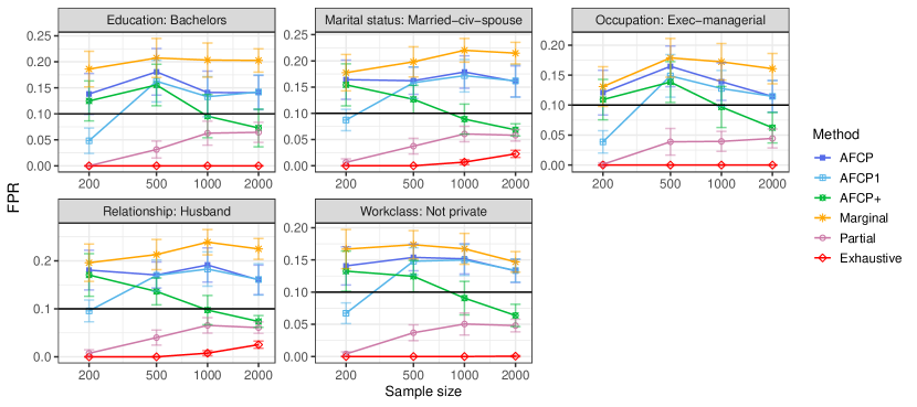
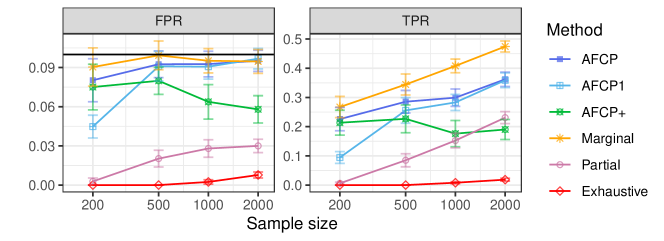
| AFCP | AFCP1 | AFCP+ | Marginal | Partial | Exhaustive | |||||||
| Sample size | FPR | TPR | FPR | TPR | FPR | TPR | FPR | TPR | FPR | TPR | FPR | TPR |
| 1 | ||||||||||||
| 200 | 0.080 (0.008) | 0.226 (0.020) | 0.045 (0.004) | 0.094 (0.010) | 0.075 (0.009) | 0.214 (0.021) | 0.090 (0.007) | 0.267 (0.018) | 0.003 (0.001) | 0.006 (0.002) | 0.000 (0.000) | 0.000 (0.000) |
| 1 | ||||||||||||
| 500 | 0.093 (0.005) | 0.285 (0.019) | 0.091 (0.006) | 0.256 (0.022) | 0.080 (0.005) | 0.227 (0.024) | 0.099 (0.006) | 0.344 (0.018) | 0.020 (0.003) | 0.085 (0.011) | 0.000 (0.000) | 0.000 (0.000) |
| 1 | ||||||||||||
| 1000 | 0.093 (0.005) | 0.299 (0.015) | 0.091 (0.005) | 0.283 (0.014) | 0.064 (0.007) | 0.176 (0.022) | 0.095 (0.005) | 0.408 (0.012) | 0.028 (0.003) | 0.153 (0.013) | 0.002 (0.001) | 0.008 (0.002) |
| 1 | ||||||||||||
| 2000 | 0.095 (0.004) | 0.362 (0.012) | 0.097 (0.004) | 0.359 (0.013) | 0.058 (0.005) | 0.190 (0.017) | 0.095 (0.005) | 0.475 (0.009) | 0.030 (0.003) | 0.231 (0.010) | 0.008 (0.001) | 0.019 (0.002) |
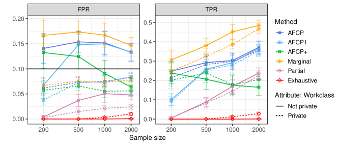
| AFCP | AFCP1 | AFCP+ | Marginal | Partial | Exhaustive | ||||||||
| Attribute: Workclass | Sample size | FPR | TPR | FPR | TPR | FPR | TPR | FPR | TPR | FPR | TPR | FPR | TPR |
| Not private | |||||||||||||
| Not private | 200 | 0.141 (0.015) | 0.248 (0.025) | 0.067 (0.008) | 0.101 (0.015) | 0.133 (0.016) | 0.238 (0.027) | 0.167 (0.015) | 0.306 (0.026) | 0.004 (0.002) | 0.005 (0.002) | 0.000 (0.000) | 0.000 (0.000) |
| Not private | 500 | 0.154 (0.010) | 0.292 (0.022) | 0.148 (0.010) | 0.258 (0.025) | 0.125 (0.012) | 0.206 (0.026) | 0.174 (0.011) | 0.380 (0.019) | 0.037 (0.006) | 0.089 (0.012) | 0.000 (0.000) | 0.000 (0.000) |
| Not private | 1000 | 0.152 (0.012) | 0.303 (0.019) | 0.150 (0.012) | 0.292 (0.018) | 0.091 (0.013) | 0.175 (0.024) | 0.167 (0.012) | 0.451 (0.019) | 0.051 (0.009) | 0.169 (0.018) | 0.000 (0.000) | 0.000 (0.000) |
| Not private | 2000 | 0.133 (0.009) | 0.371 (0.017) | 0.134 (0.009) | 0.367 (0.016) | 0.064 (0.009) | 0.164 (0.021) | 0.147 (0.008) | 0.484 (0.014) | 0.048 (0.005) | 0.238 (0.013) | 0.001 (0.001) | 0.001 (0.001) |
| Private | |||||||||||||
| Private | 200 | 0.062 (0.008) | 0.214 (0.021) | 0.038 (0.005) | 0.091 (0.014) | 0.057 (0.008) | 0.201 (0.022) | 0.067 (0.007) | 0.248 (0.019) | 0.002 (0.001) | 0.006 (0.002) | 0.000 (0.000) | 0.000 (0.000) |
| Private | 500 | 0.073 (0.005) | 0.283 (0.021) | 0.073 (0.006) | 0.254 (0.022) | 0.066 (0.005) | 0.239 (0.025) | 0.076 (0.005) | 0.324 (0.021) | 0.015 (0.003) | 0.083 (0.012) | 0.000 (0.000) | 0.000 (0.000) |
| Private | 1000 | 0.075 (0.006) | 0.298 (0.020) | 0.073 (0.006) | 0.279 (0.018) | 0.055 (0.006) | 0.178 (0.026) | 0.073 (0.004) | 0.386 (0.011) | 0.021 (0.003) | 0.144 (0.012) | 0.003 (0.001) | 0.012 (0.003) |
| Private | 2000 | 0.083 (0.004) | 0.356 (0.014) | 0.085 (0.004) | 0.353 (0.015) | 0.056 (0.005) | 0.205 (0.017) | 0.078 (0.005) | 0.468 (0.013) | 0.024 (0.003) | 0.226 (0.012) | 0.010 (0.002) | 0.028 (0.004) |
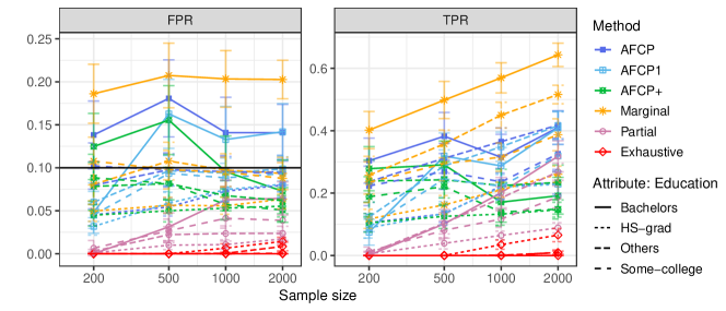
| AFCP | AFCP1 | AFCP+ | Marginal | Partial | Exhaustive | ||||||||
| Attribute: Education | Sample size | FPR | TPR | FPR | TPR | FPR | TPR | FPR | TPR | FPR | TPR | FPR | TPR |
| Bachelors | |||||||||||||
| Bachelors | 200 | 0.138 (0.020) | 0.304 (0.036) | 0.048 (0.012) | 0.075 (0.021) | 0.125 (0.019) | 0.278 (0.035) | 0.186 (0.017) | 0.402 (0.030) | 0.000 (0.000) | 0.000 (0.000) | 0.000 (0.000) | 0.000 (0.000) |
| Bachelors | 500 | 0.181 (0.022) | 0.382 (0.038) | 0.163 (0.020) | 0.319 (0.037) | 0.155 (0.020) | 0.291 (0.038) | 0.207 (0.019) | 0.498 (0.030) | 0.031 (0.008) | 0.102 (0.023) | 0.000 (0.000) | 0.000 (0.000) |
| Bachelors | 1000 | 0.141 (0.021) | 0.315 (0.037) | 0.133 (0.019) | 0.287 (0.029) | 0.095 (0.021) | 0.171 (0.032) | 0.203 (0.016) | 0.570 (0.024) | 0.063 (0.012) | 0.201 (0.024) | 0.000 (0.000) | 0.000 (0.000) |
| Bachelors | 2000 | 0.141 (0.017) | 0.410 (0.027) | 0.142 (0.016) | 0.409 (0.027) | 0.073 (0.018) | 0.192 (0.029) | 0.203 (0.011) | 0.643 (0.019) | 0.064 (0.010) | 0.318 (0.025) | 0.000 (0.000) | 0.000 (0.000) |
| HS-grad | |||||||||||||
| HS-grad | 200 | 0.045 (0.006) | 0.105 (0.015) | 0.032 (0.005) | 0.089 (0.016) | 0.045 (0.006) | 0.105 (0.015) | 0.050 (0.006) | 0.117 (0.015) | 0.001 (0.001) | 0.005 (0.003) | 0.000 (0.000) | 0.000 (0.000) |
| HS-grad | 500 | 0.054 (0.005) | 0.134 (0.013) | 0.059 (0.006) | 0.135 (0.019) | 0.050 (0.006) | 0.126 (0.020) | 0.056 (0.005) | 0.162 (0.015) | 0.010 (0.003) | 0.039 (0.009) | 0.000 (0.000) | 0.000 (0.000) |
| HS-grad | 1000 | 0.073 (0.006) | 0.223 (0.021) | 0.075 (0.007) | 0.219 (0.020) | 0.053 (0.007) | 0.133 (0.018) | 0.056 (0.005) | 0.211 (0.012) | 0.011 (0.003) | 0.064 (0.007) | 0.007 (0.003) | 0.035 (0.007) |
| HS-grad | 2000 | 0.080 (0.008) | 0.234 (0.018) | 0.081 (0.008) | 0.228 (0.019) | 0.055 (0.006) | 0.147 (0.012) | 0.064 (0.006) | 0.260 (0.013) | 0.017 (0.003) | 0.089 (0.008) | 0.014 (0.002) | 0.065 (0.011) |
| Others | |||||||||||||
| Others | 200 | 0.080 (0.014) | 0.237 (0.033) | 0.060 (0.011) | 0.123 (0.023) | 0.078 (0.014) | 0.239 (0.034) | 0.081 (0.012) | 0.257 (0.030) | 0.003 (0.001) | 0.007 (0.003) | 0.000 (0.000) | 0.000 (0.000) |
| Others | 500 | 0.098 (0.009) | 0.312 (0.024) | 0.097 (0.009) | 0.287 (0.026) | 0.082 (0.009) | 0.243 (0.029) | 0.108 (0.011) | 0.358 (0.022) | 0.022 (0.005) | 0.104 (0.017) | 0.000 (0.000) | 0.000 (0.000) |
| Others | 1000 | 0.096 (0.009) | 0.365 (0.022) | 0.094 (0.009) | 0.349 (0.023) | 0.068 (0.009) | 0.224 (0.026) | 0.097 (0.010) | 0.450 (0.021) | 0.024 (0.004) | 0.184 (0.018) | 0.001 (0.001) | 0.001 (0.001) |
| Others | 2000 | 0.095 (0.008) | 0.418 (0.022) | 0.099 (0.007) | 0.416 (0.022) | 0.062 (0.008) | 0.234 (0.028) | 0.093 (0.009) | 0.516 (0.015) | 0.024 (0.004) | 0.268 (0.014) | 0.008 (0.003) | 0.009 (0.002) |
| Some-college | |||||||||||||
| Some-college | 200 | 0.102 (0.013) | 0.223 (0.032) | 0.045 (0.008) | 0.091 (0.018) | 0.088 (0.014) | 0.188 (0.032) | 0.108 (0.014) | 0.235 (0.033) | 0.007 (0.004) | 0.014 (0.007) | 0.000 (0.000) | 0.000 (0.000) |
| Some-college | 500 | 0.097 (0.010) | 0.269 (0.029) | 0.093 (0.011) | 0.245 (0.030) | 0.082 (0.009) | 0.221 (0.030) | 0.098 (0.011) | 0.294 (0.027) | 0.027 (0.007) | 0.081 (0.015) | 0.000 (0.000) | 0.000 (0.000) |
| Some-college | 1000 | 0.095 (0.009) | 0.236 (0.022) | 0.088 (0.008) | 0.222 (0.022) | 0.057 (0.009) | 0.139 (0.022) | 0.095 (0.009) | 0.315 (0.023) | 0.041 (0.006) | 0.117 (0.013) | 0.000 (0.000) | 0.000 (0.000) |
| Some-college | 2000 | 0.093 (0.011) | 0.326 (0.025) | 0.093 (0.011) | 0.319 (0.025) | 0.051 (0.006) | 0.149 (0.016) | 0.088 (0.009) | 0.387 (0.026) | 0.039 (0.006) | 0.188 (0.018) | 0.001 (0.001) | 0.009 (0.004) |
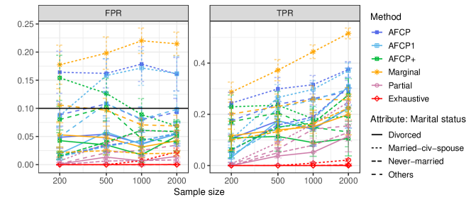
| AFCP | AFCP1 | AFCP+ | Marginal | Partial | Exhaustive | ||||||||
| Attribute: Marital status | Sample size | FPR | TPR | FPR | TPR | FPR | TPR | FPR | TPR | FPR | TPR | FPR | TPR |
| Divorced | |||||||||||||
| Divorced | 200 | 0.049 (0.010) | 0.105 (0.027) | 0.020 (0.006) | 0.032 (0.014) | 0.043 (0.010) | 0.107 (0.027) | 0.053 (0.011) | 0.116 (0.028) | 0.001 (0.001) | 0.000 (0.000) | 0.000 (0.000) | 0.000 (0.000) |
| Divorced | 500 | 0.054 (0.012) | 0.174 (0.038) | 0.058 (0.013) | 0.174 (0.038) | 0.035 (0.009) | 0.114 (0.029) | 0.048 (0.010) | 0.139 (0.030) | 0.013 (0.006) | 0.037 (0.016) | 0.000 (0.000) | 0.000 (0.000) |
| Divorced | 1000 | 0.037 (0.010) | 0.141 (0.033) | 0.036 (0.011) | 0.144 (0.032) | 0.017 (0.007) | 0.089 (0.027) | 0.031 (0.009) | 0.151 (0.032) | 0.006 (0.005) | 0.052 (0.020) | 0.000 (0.000) | 0.000 (0.000) |
| Divorced | 2000 | 0.054 (0.011) | 0.224 (0.039) | 0.054 (0.010) | 0.224 (0.039) | 0.051 (0.013) | 0.105 (0.034) | 0.043 (0.009) | 0.199 (0.040) | 0.015 (0.005) | 0.114 (0.030) | 0.000 (0.000) | 0.000 (0.000) |
| Married-civ-spouse | |||||||||||||
| Married-civ-spouse | 200 | 0.164 (0.019) | 0.243 (0.021) | 0.087 (0.010) | 0.103 (0.012) | 0.154 (0.020) | 0.229 (0.023) | 0.178 (0.017) | 0.286 (0.020) | 0.007 (0.003) | 0.007 (0.002) | 0.000 (0.000) | 0.000 (0.000) |
| Married-civ-spouse | 500 | 0.162 (0.013) | 0.299 (0.022) | 0.158 (0.015) | 0.266 (0.025) | 0.127 (0.013) | 0.236 (0.027) | 0.198 (0.014) | 0.372 (0.021) | 0.037 (0.008) | 0.090 (0.012) | 0.000 (0.000) | 0.000 (0.000) |
| Married-civ-spouse | 1000 | 0.179 (0.015) | 0.315 (0.018) | 0.172 (0.015) | 0.297 (0.017) | 0.089 (0.014) | 0.182 (0.024) | 0.220 (0.011) | 0.444 (0.013) | 0.061 (0.007) | 0.162 (0.014) | 0.007 (0.002) | 0.009 (0.002) |
| Married-civ-spouse | 2000 | 0.161 (0.015) | 0.375 (0.015) | 0.162 (0.016) | 0.371 (0.015) | 0.068 (0.006) | 0.192 (0.017) | 0.215 (0.010) | 0.516 (0.011) | 0.058 (0.006) | 0.247 (0.012) | 0.023 (0.003) | 0.021 (0.003) |
| Never-married | |||||||||||||
| Never-married | 200 | 0.015 (0.003) | 0.059 (0.016) | 0.014 (0.003) | 0.041 (0.014) | 0.015 (0.003) | 0.063 (0.016) | 0.022 (0.004) | 0.100 (0.021) | 0.000 (0.000) | 0.000 (0.000) | 0.000 (0.000) | 0.000 (0.000) |
| Never-married | 500 | 0.034 (0.006) | 0.158 (0.023) | 0.032 (0.006) | 0.147 (0.022) | 0.040 (0.008) | 0.150 (0.022) | 0.025 (0.004) | 0.132 (0.020) | 0.006 (0.002) | 0.050 (0.010) | 0.000 (0.000) | 0.000 (0.000) |
| Never-married | 1000 | 0.043 (0.009) | 0.190 (0.024) | 0.043 (0.009) | 0.182 (0.023) | 0.061 (0.009) | 0.166 (0.025) | 0.019 (0.003) | 0.163 (0.019) | 0.007 (0.002) | 0.079 (0.014) | 0.000 (0.000) | 0.000 (0.000) |
| Never-married | 2000 | 0.055 (0.009) | 0.307 (0.036) | 0.056 (0.009) | 0.309 (0.036) | 0.059 (0.008) | 0.275 (0.032) | 0.020 (0.003) | 0.224 (0.023) | 0.008 (0.002) | 0.129 (0.017) | 0.000 (0.000) | 0.002 (0.002) |
| Others | |||||||||||||
| Others | 200 | 0.089 (0.012) | 0.175 (0.028) | 0.050 (0.009) | 0.049 (0.011) | 0.080 (0.012) | 0.171 (0.029) | 0.106 (0.015) | 0.201 (0.029) | 0.002 (0.001) | 0.005 (0.003) | 0.000 (0.000) | 0.000 (0.000) |
| Others | 500 | 0.108 (0.011) | 0.240 (0.025) | 0.108 (0.011) | 0.225 (0.021) | 0.102 (0.012) | 0.205 (0.023) | 0.097 (0.011) | 0.230 (0.025) | 0.021 (0.006) | 0.063 (0.014) | 0.000 (0.000) | 0.000 (0.000) |
| Others | 1000 | 0.080 (0.011) | 0.262 (0.031) | 0.081 (0.011) | 0.255 (0.032) | 0.046 (0.010) | 0.149 (0.036) | 0.071 (0.006) | 0.259 (0.027) | 0.025 (0.005) | 0.142 (0.025) | 0.000 (0.000) | 0.000 (0.000) |
| Others | 2000 | 0.093 (0.012) | 0.288 (0.022) | 0.098 (0.013) | 0.299 (0.022) | 0.039 (0.007) | 0.131 (0.029) | 0.069 (0.010) | 0.256 (0.024) | 0.035 (0.007) | 0.155 (0.020) | 0.000 (0.000) | 0.000 (0.000) |
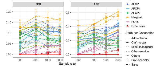
| AFCP | AFCP1 | AFCP+ | Marginal | Partial | Exhaustive | ||||||||
| Attribute: Occupation | Sample size | FPR | TPR | FPR | TPR | FPR | TPR | FPR | TPR | FPR | TPR | FPR | TPR |
| Adm-clerical | |||||||||||||
| Adm-clerical | 200 | 0.090 (0.015) | 0.206 (0.027) | 0.058 (0.014) | 0.126 (0.032) | 0.077 (0.015) | 0.183 (0.028) | 0.113 (0.018) | 0.239 (0.028) | 0.003 (0.002) | 0.010 (0.010) | 0.000 (0.000) | 0.000 (0.000) |
| Adm-clerical | 500 | 0.122 (0.014) | 0.242 (0.030) | 0.107 (0.014) | 0.192 (0.030) | 0.118 (0.015) | 0.209 (0.031) | 0.136 (0.015) | 0.321 (0.028) | 0.037 (0.012) | 0.069 (0.020) | 0.000 (0.000) | 0.000 (0.000) |
| Adm-clerical | 1000 | 0.108 (0.014) | 0.248 (0.027) | 0.112 (0.015) | 0.245 (0.025) | 0.078 (0.015) | 0.128 (0.022) | 0.093 (0.012) | 0.281 (0.025) | 0.042 (0.010) | 0.133 (0.022) | 0.000 (0.000) | 0.000 (0.000) |
| Adm-clerical | 2000 | 0.106 (0.014) | 0.322 (0.033) | 0.102 (0.014) | 0.312 (0.032) | 0.059 (0.011) | 0.132 (0.027) | 0.086 (0.012) | 0.352 (0.029) | 0.041 (0.007) | 0.176 (0.027) | 0.000 (0.000) | 0.000 (0.000) |
| Craft-repair | |||||||||||||
| Craft-repair | 200 | 0.103 (0.017) | 0.176 (0.030) | 0.050 (0.012) | 0.073 (0.016) | 0.099 (0.016) | 0.165 (0.029) | 0.108 (0.015) | 0.183 (0.029) | 0.004 (0.004) | 0.008 (0.005) | 0.000 (0.000) | 0.000 (0.000) |
| Craft-repair | 500 | 0.075 (0.011) | 0.187 (0.023) | 0.075 (0.013) | 0.182 (0.024) | 0.079 (0.011) | 0.160 (0.023) | 0.097 (0.011) | 0.230 (0.023) | 0.023 (0.006) | 0.071 (0.014) | 0.000 (0.000) | 0.000 (0.000) |
| Craft-repair | 1000 | 0.128 (0.014) | 0.242 (0.027) | 0.123 (0.013) | 0.229 (0.028) | 0.065 (0.013) | 0.131 (0.023) | 0.134 (0.012) | 0.278 (0.021) | 0.050 (0.009) | 0.104 (0.015) | 0.008 (0.004) | 0.027 (0.009) |
| Craft-repair | 2000 | 0.102 (0.012) | 0.270 (0.022) | 0.099 (0.012) | 0.262 (0.022) | 0.065 (0.009) | 0.168 (0.017) | 0.123 (0.012) | 0.346 (0.020) | 0.035 (0.005) | 0.163 (0.013) | 0.010 (0.003) | 0.065 (0.010) |
| Exec-managerial | |||||||||||||
| Exec-managerial | 200 | 0.121 (0.019) | 0.248 (0.033) | 0.039 (0.009) | 0.079 (0.021) | 0.109 (0.017) | 0.237 (0.033) | 0.131 (0.017) | 0.279 (0.031) | 0.001 (0.001) | 0.003 (0.003) | 0.000 (0.000) | 0.000 (0.000) |
| Exec-managerial | 500 | 0.165 (0.017) | 0.362 (0.033) | 0.149 (0.018) | 0.298 (0.033) | 0.139 (0.017) | 0.282 (0.034) | 0.179 (0.016) | 0.439 (0.025) | 0.039 (0.011) | 0.103 (0.017) | 0.000 (0.000) | 0.000 (0.000) |
| Exec-managerial | 1000 | 0.139 (0.016) | 0.340 (0.031) | 0.128 (0.015) | 0.300 (0.024) | 0.097 (0.017) | 0.201 (0.038) | 0.172 (0.015) | 0.517 (0.021) | 0.040 (0.008) | 0.193 (0.023) | 0.000 (0.000) | 0.000 (0.000) |
| Exec-managerial | 2000 | 0.115 (0.013) | 0.442 (0.021) | 0.115 (0.013) | 0.440 (0.021) | 0.062 (0.013) | 0.231 (0.030) | 0.161 (0.013) | 0.611 (0.018) | 0.044 (0.008) | 0.319 (0.018) | 0.000 (0.000) | 0.000 (0.000) |
| Other-service | |||||||||||||
| Other-service | 200 | 0.026 (0.007) | 0.114 (0.034) | 0.016 (0.006) | 0.050 (0.022) | 0.023 (0.007) | 0.101 (0.034) | 0.025 (0.006) | 0.131 (0.036) | 0.000 (0.000) | 0.000 (0.000) | 0.000 (0.000) | 0.000 (0.000) |
| Other-service | 500 | 0.065 (0.012) | 0.249 (0.055) | 0.071 (0.012) | 0.269 (0.053) | 0.041 (0.008) | 0.180 (0.044) | 0.044 (0.006) | 0.242 (0.045) | 0.009 (0.004) | 0.082 (0.028) | 0.000 (0.000) | 0.000 (0.000) |
| Other-service | 1000 | 0.039 (0.008) | 0.118 (0.028) | 0.038 (0.008) | 0.129 (0.033) | 0.034 (0.007) | 0.069 (0.026) | 0.035 (0.006) | 0.129 (0.040) | 0.012 (0.004) | 0.049 (0.018) | 0.000 (0.000) | 0.000 (0.000) |
| Other-service | 2000 | 0.070 (0.011) | 0.253 (0.042) | 0.073 (0.011) | 0.253 (0.042) | 0.040 (0.009) | 0.107 (0.025) | 0.028 (0.006) | 0.201 (0.029) | 0.013 (0.004) | 0.062 (0.018) | 0.000 (0.000) | 0.000 (0.000) |
| Others | |||||||||||||
| Others | 200 | 0.058 (0.012) | 0.141 (0.021) | 0.059 (0.012) | 0.118 (0.024) | 0.056 (0.012) | 0.137 (0.021) | 0.060 (0.012) | 0.151 (0.024) | 0.005 (0.002) | 0.007 (0.004) | 0.000 (0.000) | 0.000 (0.000) |
| Others | 500 | 0.064 (0.009) | 0.187 (0.024) | 0.069 (0.009) | 0.195 (0.024) | 0.054 (0.010) | 0.163 (0.026) | 0.058 (0.008) | 0.187 (0.023) | 0.011 (0.004) | 0.047 (0.011) | 0.000 (0.000) | 0.000 (0.000) |
| Others | 1000 | 0.070 (0.007) | 0.214 (0.019) | 0.073 (0.007) | 0.221 (0.022) | 0.054 (0.008) | 0.146 (0.017) | 0.050 (0.007) | 0.243 (0.013) | 0.010 (0.003) | 0.081 (0.010) | 0.004 (0.002) | 0.027 (0.009) |
| Others | 2000 | 0.071 (0.008) | 0.225 (0.018) | 0.077 (0.010) | 0.229 (0.018) | 0.059 (0.005) | 0.161 (0.017) | 0.062 (0.008) | 0.259 (0.016) | 0.017 (0.003) | 0.102 (0.012) | 0.023 (0.004) | 0.061 (0.009) |
| Prof-specialty | |||||||||||||
| Prof-specialty | 200 | 0.094 (0.017) | 0.243 (0.032) | 0.040 (0.012) | 0.079 (0.020) | 0.091 (0.016) | 0.232 (0.033) | 0.125 (0.017) | 0.308 (0.029) | 0.000 (0.000) | 0.000 (0.000) | 0.000 (0.000) | 0.000 (0.000) |
| Prof-specialty | 500 | 0.136 (0.024) | 0.309 (0.033) | 0.129 (0.019) | 0.275 (0.034) | 0.118 (0.021) | 0.225 (0.031) | 0.147 (0.027) | 0.385 (0.029) | 0.018 (0.006) | 0.086 (0.015) | 0.000 (0.000) | 0.000 (0.000) |
| Prof-specialty | 1000 | 0.122 (0.016) | 0.332 (0.018) | 0.120 (0.016) | 0.321 (0.019) | 0.074 (0.015) | 0.193 (0.026) | 0.159 (0.018) | 0.464 (0.019) | 0.039 (0.010) | 0.163 (0.018) | 0.000 (0.000) | 0.000 (0.000) |
| Prof-specialty | 2000 | 0.131 (0.013) | 0.411 (0.024) | 0.131 (0.013) | 0.404 (0.026) | 0.073 (0.014) | 0.205 (0.029) | 0.167 (0.012) | 0.562 (0.021) | 0.037 (0.008) | 0.262 (0.017) | 0.000 (0.000) | 0.000 (0.000) |
| Sales | |||||||||||||
| Sales | 200 | 0.110 (0.016) | 0.326 (0.035) | 0.032 (0.008) | 0.120 (0.022) | 0.105 (0.016) | 0.306 (0.037) | 0.127 (0.015) | 0.415 (0.036) | 0.002 (0.002) | 0.013 (0.007) | 0.000 (0.000) | 0.000 (0.000) |
| Sales | 500 | 0.086 (0.015) | 0.344 (0.035) | 0.084 (0.014) | 0.327 (0.037) | 0.071 (0.011) | 0.286 (0.038) | 0.126 (0.019) | 0.428 (0.034) | 0.021 (0.005) | 0.124 (0.024) | 0.000 (0.000) | 0.000 (0.000) |
| Sales | 1000 | 0.103 (0.016) | 0.382 (0.025) | 0.091 (0.015) | 0.357 (0.024) | 0.072 (0.013) | 0.221 (0.032) | 0.128 (0.012) | 0.535 (0.025) | 0.036 (0.008) | 0.218 (0.021) | 0.000 (0.000) | 0.000 (0.000) |
| Sales | 2000 | 0.112 (0.014) | 0.404 (0.031) | 0.114 (0.014) | 0.402 (0.031) | 0.045 (0.009) | 0.185 (0.032) | 0.111 (0.011) | 0.548 (0.021) | 0.041 (0.009) | 0.278 (0.025) | 0.000 (0.000) | 0.000 (0.000) |
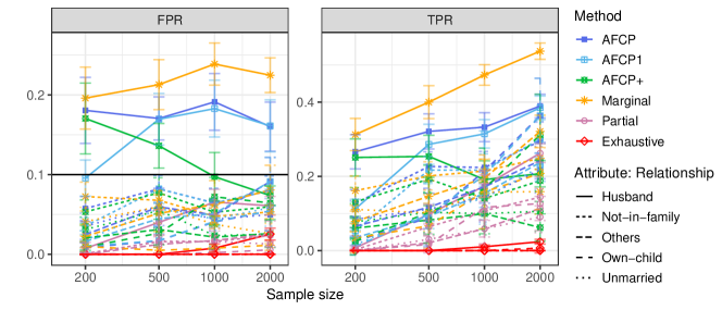
| AFCP | AFCP1 | AFCP+ | Marginal | Partial | Exhaustive | ||||||||
| Attribute: Relationship | Sample size | FPR | TPR | FPR | TPR | FPR | TPR | FPR | TPR | FPR | TPR | FPR | TPR |
| Husband | |||||||||||||
| Husband | 200 | 0.181 (0.021) | 0.266 (0.023) | 0.096 (0.011) | 0.112 (0.013) | 0.170 (0.022) | 0.251 (0.025) | 0.196 (0.019) | 0.313 (0.022) | 0.007 (0.004) | 0.007 (0.003) | 0.000 (0.000) | 0.000 (0.000) |
| Husband | 500 | 0.170 (0.014) | 0.321 (0.024) | 0.169 (0.016) | 0.286 (0.027) | 0.136 (0.014) | 0.254 (0.028) | 0.213 (0.016) | 0.400 (0.022) | 0.040 (0.008) | 0.098 (0.013) | 0.000 (0.000) | 0.000 (0.000) |
| Husband | 1000 | 0.191 (0.018) | 0.332 (0.019) | 0.183 (0.018) | 0.314 (0.019) | 0.097 (0.015) | 0.191 (0.025) | 0.239 (0.013) | 0.473 (0.014) | 0.066 (0.008) | 0.174 (0.015) | 0.008 (0.003) | 0.010 (0.002) |
| Husband | 2000 | 0.160 (0.015) | 0.389 (0.016) | 0.161 (0.016) | 0.385 (0.016) | 0.074 (0.006) | 0.207 (0.018) | 0.225 (0.011) | 0.537 (0.011) | 0.061 (0.006) | 0.262 (0.013) | 0.025 (0.004) | 0.024 (0.003) |
| Not-in-family | |||||||||||||
| Not-in-family | 200 | 0.057 (0.007) | 0.127 (0.018) | 0.035 (0.005) | 0.054 (0.010) | 0.053 (0.007) | 0.131 (0.019) | 0.072 (0.009) | 0.161 (0.020) | 0.001 (0.001) | 0.003 (0.002) | 0.000 (0.000) | 0.000 (0.000) |
| Not-in-family | 500 | 0.082 (0.009) | 0.227 (0.020) | 0.082 (0.008) | 0.217 (0.018) | 0.077 (0.009) | 0.193 (0.019) | 0.068 (0.006) | 0.201 (0.019) | 0.016 (0.003) | 0.064 (0.009) | 0.000 (0.000) | 0.000 (0.000) |
| Not-in-family | 1000 | 0.064 (0.009) | 0.224 (0.022) | 0.064 (0.009) | 0.217 (0.022) | 0.053 (0.009) | 0.141 (0.022) | 0.048 (0.005) | 0.215 (0.016) | 0.016 (0.004) | 0.108 (0.012) | 0.000 (0.000) | 0.000 (0.000) |
| Not-in-family | 2000 | 0.080 (0.009) | 0.295 (0.026) | 0.081 (0.009) | 0.300 (0.025) | 0.060 (0.008) | 0.188 (0.028) | 0.053 (0.004) | 0.248 (0.015) | 0.023 (0.004) | 0.144 (0.012) | 0.000 (0.000) | 0.000 (0.000) |
| Others | |||||||||||||
| Others | 200 | 0.025 (0.008) | 0.066 (0.013) | 0.016 (0.007) | 0.035 (0.010) | 0.021 (0.008) | 0.061 (0.014) | 0.022 (0.007) | 0.078 (0.014) | 0.000 (0.000) | 0.000 (0.000) | 0.000 (0.000) | 0.000 (0.000) |
| Others | 500 | 0.059 (0.012) | 0.117 (0.019) | 0.045 (0.009) | 0.093 (0.017) | 0.031 (0.010) | 0.082 (0.019) | 0.051 (0.012) | 0.146 (0.021) | 0.012 (0.006) | 0.021 (0.009) | 0.000 (0.000) | 0.000 (0.000) |
| Others | 1000 | 0.049 (0.008) | 0.172 (0.022) | 0.051 (0.008) | 0.154 (0.019) | 0.021 (0.008) | 0.100 (0.027) | 0.062 (0.015) | 0.195 (0.026) | 0.017 (0.006) | 0.059 (0.011) | 0.000 (0.000) | 0.000 (0.000) |
| Others | 2000 | 0.091 (0.015) | 0.243 (0.025) | 0.091 (0.015) | 0.237 (0.025) | 0.026 (0.009) | 0.062 (0.018) | 0.081 (0.015) | 0.321 (0.022) | 0.026 (0.008) | 0.114 (0.016) | 0.000 (0.000) | 0.000 (0.000) |
| Own-child | |||||||||||||
| Own-child | 200 | 0.008 (0.003) | 0.025 (0.018) | 0.010 (0.003) | 0.011 (0.011) | 0.009 (0.003) | 0.025 (0.018) | 0.010 (0.003) | 0.033 (0.020) | 0.001 (0.001) | 0.000 (0.000) | 0.000 (0.000) | 0.000 (0.000) |
| Own-child | 500 | 0.017 (0.009) | 0.089 (0.040) | 0.017 (0.009) | 0.097 (0.042) | 0.026 (0.009) | 0.103 (0.041) | 0.005 (0.002) | 0.067 (0.030) | 0.000 (0.000) | 0.017 (0.012) | 0.000 (0.000) | 0.000 (0.000) |
| Own-child | 1000 | 0.041 (0.014) | 0.214 (0.060) | 0.041 (0.014) | 0.203 (0.060) | 0.072 (0.012) | 0.167 (0.055) | 0.008 (0.002) | 0.158 (0.050) | 0.002 (0.001) | 0.117 (0.049) | 0.000 (0.000) | 0.000 (0.000) |
| Own-child | 2000 | 0.054 (0.012) | 0.363 (0.050) | 0.054 (0.012) | 0.363 (0.050) | 0.064 (0.011) | 0.312 (0.055) | 0.011 (0.003) | 0.208 (0.049) | 0.006 (0.002) | 0.127 (0.036) | 0.000 (0.000) | 0.007 (0.007) |
| Unmarried | |||||||||||||
| Unmarried | 200 | 0.035 (0.008) | 0.084 (0.025) | 0.018 (0.006) | 0.015 (0.011) | 0.031 (0.008) | 0.078 (0.024) | 0.041 (0.009) | 0.111 (0.029) | 0.000 (0.000) | 0.000 (0.000) | 0.000 (0.000) | 0.000 (0.000) |
| Unmarried | 500 | 0.060 (0.010) | 0.112 (0.027) | 0.057 (0.010) | 0.102 (0.027) | 0.055 (0.011) | 0.103 (0.027) | 0.060 (0.010) | 0.101 (0.025) | 0.017 (0.007) | 0.030 (0.013) | 0.000 (0.000) | 0.000 (0.000) |
| Unmarried | 1000 | 0.044 (0.007) | 0.144 (0.034) | 0.044 (0.009) | 0.142 (0.035) | 0.024 (0.007) | 0.099 (0.029) | 0.038 (0.007) | 0.157 (0.031) | 0.016 (0.004) | 0.059 (0.023) | 0.000 (0.000) | 0.000 (0.000) |
| Unmarried | 2000 | 0.050 (0.010) | 0.218 (0.031) | 0.058 (0.012) | 0.226 (0.031) | 0.025 (0.008) | 0.106 (0.027) | 0.026 (0.006) | 0.159 (0.030) | 0.013 (0.005) | 0.090 (0.021) | 0.000 (0.000) | 0.000 (0.000) |
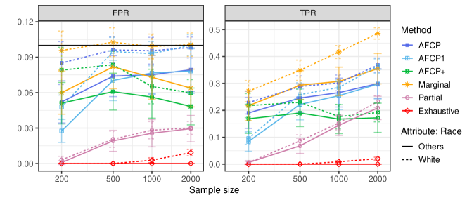
| AFCP | AFCP1 | AFCP+ | Marginal | Partial | Exhaustive | ||||||||
| Attribute: Race | Sample size | FPR | TPR | FPR | TPR | FPR | TPR | FPR | TPR | FPR | TPR | FPR | TPR |
| Others | |||||||||||||
| Others | 200 | 0.052 (0.009) | 0.190 (0.029) | 0.028 (0.005) | 0.084 (0.018) | 0.051 (0.009) | 0.169 (0.027) | 0.060 (0.009) | 0.217 (0.028) | 0.001 (0.001) | 0.006 (0.004) | 0.000 (0.000) | 0.000 (0.000) |
| Others | 500 | 0.074 (0.009) | 0.246 (0.026) | 0.070 (0.009) | 0.222 (0.029) | 0.061 (0.008) | 0.190 (0.025) | 0.082 (0.009) | 0.293 (0.027) | 0.019 (0.004) | 0.068 (0.014) | 0.000 (0.000) | 0.000 (0.000) |
| Others | 1000 | 0.075 (0.008) | 0.266 (0.027) | 0.077 (0.009) | 0.254 (0.026) | 0.056 (0.009) | 0.167 (0.027) | 0.073 (0.009) | 0.308 (0.026) | 0.026 (0.006) | 0.144 (0.019) | 0.000 (0.000) | 0.000 (0.000) |
| Others | 2000 | 0.079 (0.009) | 0.299 (0.027) | 0.078 (0.009) | 0.298 (0.028) | 0.048 (0.008) | 0.172 (0.027) | 0.064 (0.008) | 0.355 (0.028) | 0.029 (0.006) | 0.209 (0.022) | 0.000 (0.000) | 0.000 (0.000) |
| White | |||||||||||||
| White | 200 | 0.085 (0.009) | 0.229 (0.021) | 0.048 (0.005) | 0.095 (0.011) | 0.079 (0.010) | 0.218 (0.022) | 0.096 (0.008) | 0.271 (0.020) | 0.003 (0.001) | 0.006 (0.002) | 0.000 (0.000) | 0.000 (0.000) |
| White | 500 | 0.096 (0.005) | 0.289 (0.020) | 0.095 (0.006) | 0.258 (0.022) | 0.084 (0.006) | 0.230 (0.024) | 0.103 (0.006) | 0.349 (0.019) | 0.021 (0.003) | 0.086 (0.011) | 0.000 (0.000) | 0.000 (0.000) |
| White | 1000 | 0.095 (0.006) | 0.302 (0.015) | 0.093 (0.005) | 0.285 (0.014) | 0.065 (0.007) | 0.177 (0.023) | 0.099 (0.005) | 0.417 (0.012) | 0.028 (0.004) | 0.153 (0.013) | 0.003 (0.001) | 0.009 (0.002) |
| White | 2000 | 0.098 (0.004) | 0.368 (0.013) | 0.100 (0.004) | 0.365 (0.013) | 0.060 (0.006) | 0.192 (0.017) | 0.101 (0.005) | 0.486 (0.011) | 0.030 (0.003) | 0.233 (0.011) | 0.009 (0.001) | 0.020 (0.003) |
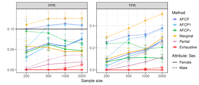
| AFCP | AFCP1 | AFCP+ | Marginal | Partial | Exhaustive | ||||||||
| Attribute: Sex | Sample size | FPR | TPR | FPR | TPR | FPR | TPR | FPR | TPR | FPR | TPR | FPR | TPR |
| Female | |||||||||||||
| Female | 200 | 0.047 (0.007) | 0.077 (0.013) | 0.031 (0.005) | 0.035 (0.008) | 0.043 (0.007) | 0.072 (0.014) | 0.057 (0.008) | 0.095 (0.014) | 0.001 (0.000) | 0.000 (0.000) | 0.000 (0.000) | 0.000 (0.000) |
| Female | 500 | 0.065 (0.007) | 0.144 (0.016) | 0.061 (0.007) | 0.123 (0.014) | 0.063 (0.008) | 0.110 (0.016) | 0.055 (0.005) | 0.159 (0.018) | 0.013 (0.003) | 0.038 (0.009) | 0.000 (0.000) | 0.000 (0.000) |
| Female | 1000 | 0.058 (0.008) | 0.182 (0.018) | 0.058 (0.007) | 0.170 (0.017) | 0.051 (0.007) | 0.113 (0.021) | 0.044 (0.005) | 0.187 (0.018) | 0.016 (0.003) | 0.073 (0.009) | 0.000 (0.000) | 0.000 (0.000) |
| Female | 2000 | 0.075 (0.007) | 0.266 (0.019) | 0.077 (0.007) | 0.265 (0.020) | 0.047 (0.007) | 0.106 (0.018) | 0.045 (0.005) | 0.290 (0.018) | 0.020 (0.003) | 0.117 (0.010) | 0.000 (0.000) | 0.000 (0.000) |
| Male | |||||||||||||
| Male | 200 | 0.100 (0.012) | 0.252 (0.022) | 0.054 (0.006) | 0.105 (0.012) | 0.095 (0.012) | 0.239 (0.024) | 0.111 (0.010) | 0.297 (0.021) | 0.004 (0.002) | 0.007 (0.002) | 0.000 (0.000) | 0.000 (0.000) |
| Male | 500 | 0.109 (0.007) | 0.310 (0.021) | 0.109 (0.008) | 0.279 (0.024) | 0.090 (0.006) | 0.247 (0.026) | 0.126 (0.008) | 0.377 (0.020) | 0.024 (0.004) | 0.093 (0.012) | 0.000 (0.000) | 0.000 (0.000) |
| Male | 1000 | 0.114 (0.007) | 0.321 (0.017) | 0.110 (0.007) | 0.304 (0.017) | 0.071 (0.008) | 0.187 (0.024) | 0.126 (0.007) | 0.448 (0.013) | 0.035 (0.004) | 0.167 (0.014) | 0.004 (0.001) | 0.009 (0.002) |
| Male | 2000 | 0.109 (0.006) | 0.379 (0.014) | 0.110 (0.006) | 0.376 (0.014) | 0.065 (0.006) | 0.205 (0.018) | 0.126 (0.007) | 0.507 (0.010) | 0.037 (0.003) | 0.251 (0.012) | 0.013 (0.002) | 0.022 (0.003) |
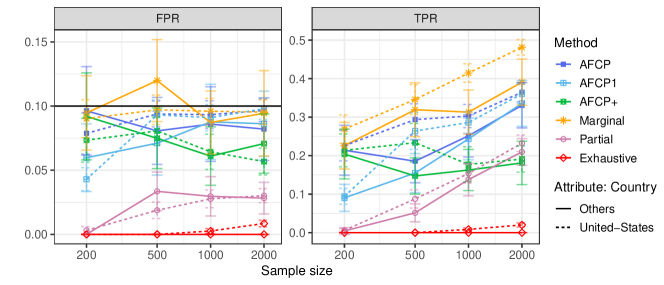
| AFCP | AFCP1 | AFCP+ | Marginal | Partial | Exhaustive | ||||||||
| Attribute: Country | Sample size | FPR | TPR | FPR | TPR | FPR | TPR | FPR | TPR | FPR | TPR | FPR | TPR |
| Others | |||||||||||||
| Others | 200 | 0.096 (0.017) | 0.214 (0.032) | 0.060 (0.013) | 0.090 (0.018) | 0.092 (0.017) | 0.204 (0.032) | 0.095 (0.014) | 0.226 (0.030) | 0.000 (0.000) | 0.004 (0.004) | 0.000 (0.000) | 0.000 (0.000) |
| Others | 500 | 0.081 (0.013) | 0.186 (0.028) | 0.071 (0.012) | 0.155 (0.025) | 0.075 (0.012) | 0.147 (0.024) | 0.120 (0.016) | 0.319 (0.035) | 0.034 (0.008) | 0.051 (0.012) | 0.000 (0.000) | 0.000 (0.000) |
| Others | 1000 | 0.086 (0.015) | 0.252 (0.028) | 0.088 (0.015) | 0.243 (0.027) | 0.061 (0.011) | 0.163 (0.027) | 0.087 (0.012) | 0.313 (0.029) | 0.030 (0.008) | 0.138 (0.021) | 0.000 (0.000) | 0.000 (0.000) |
| Others | 2000 | 0.082 (0.012) | 0.331 (0.029) | 0.086 (0.013) | 0.336 (0.030) | 0.071 (0.012) | 0.181 (0.028) | 0.094 (0.017) | 0.391 (0.030) | 0.028 (0.006) | 0.210 (0.017) | 0.000 (0.000) | 0.000 (0.000) |
| United-States | |||||||||||||
| United-States | 200 | 0.079 (0.008) | 0.226 (0.020) | 0.043 (0.004) | 0.094 (0.010) | 0.073 (0.009) | 0.214 (0.021) | 0.090 (0.007) | 0.269 (0.018) | 0.003 (0.001) | 0.006 (0.002) | 0.000 (0.000) | 0.000 (0.000) |
| United-States | 500 | 0.094 (0.005) | 0.294 (0.021) | 0.093 (0.006) | 0.264 (0.024) | 0.081 (0.005) | 0.234 (0.025) | 0.097 (0.006) | 0.346 (0.019) | 0.019 (0.003) | 0.088 (0.012) | 0.000 (0.000) | 0.000 (0.000) |
| United-States | 1000 | 0.093 (0.005) | 0.303 (0.015) | 0.091 (0.005) | 0.286 (0.014) | 0.064 (0.007) | 0.177 (0.023) | 0.096 (0.005) | 0.415 (0.012) | 0.028 (0.003) | 0.154 (0.012) | 0.003 (0.001) | 0.009 (0.002) |
| United-States | 2000 | 0.097 (0.004) | 0.365 (0.012) | 0.098 (0.004) | 0.360 (0.013) | 0.057 (0.005) | 0.191 (0.017) | 0.095 (0.005) | 0.481 (0.010) | 0.030 (0.003) | 0.232 (0.011) | 0.008 (0.001) | 0.020 (0.003) |