m o \IfNoValueTF#2 \NewDocumentCommand\Probm o \IfNoValueTF#2 \NewDocumentCommand\costoC\IfValueT#1_#1 \NewDocumentCommand\costHorizonPredSetm o\cost^#1\IfValueT#2(\infoVec_#2) \NewDocumentCommand\errorProcessmE_#1 \NewDocumentCommand\tHistoryB
[1] organization=Department of Information Technology, Uppsala University, addressline=Box 337, postcode=751 05, city=Uppsala, country=Sweden,
Certified Inventory Control of Critical Resources111This work was supported in part by the Swedish Research Council under contract 2021-05022.
Abstract
Inventory control is subject to service-level requirements, in which sufficient stock levels must be maintained despite an unknown demand. We propose a data-driven order policy that certifies any prescribed service level under minimal assumptions on the unknown demand process. The policy achieves this using any online learning method along with integral action. We further propose an inference method that is valid in finite samples. The properties and theoretical guarantees of the method are illustrated using both synthetic and real-world data.
keywords:
inventory control, forecasting , policy cost inference , policy certification1 Introduction
Inventory control using discrete-time models is a well-studied problem, where orders of items to hold in stock must anticipate future demand [1, 2]. By defining the costs of insufficient stocks, it is possible to find cost-minimizing policies using dynamic programming [3, 4, 5]. In practice, however, maintaining a certain service level of an inventory control system is a greater priority than cost minimization [6, 7]. Under certain restrictive assumptions on the demand process – such as memoryless and identically distributed demand – there are explicit formulations of the duality between service levels and costs [8]. Efforts to relax such assumptions can be found in [9, 10]. When the unknown demand distribution is learned from data, it is possible to provide probabilistic guarantees on the service level of an order policy in the special case of no stock being held between time periods [11, 12].
In this letter, we formulate an inventory control relaxing most assumptions on the demand process and allowing for arbitrary time dependence of this process, while providing order policies with certifiable service-level guarantees. The relaxation is relevant in several critical inventory control problems where service levels are important, such as hospital inventory control [13, 14].

We consider the management of a single item type with stock level at time instant by determining an order of additional units. Between and , items in stock are consumed by an unknown demand process . A critical stock event occurs if
| (1) |
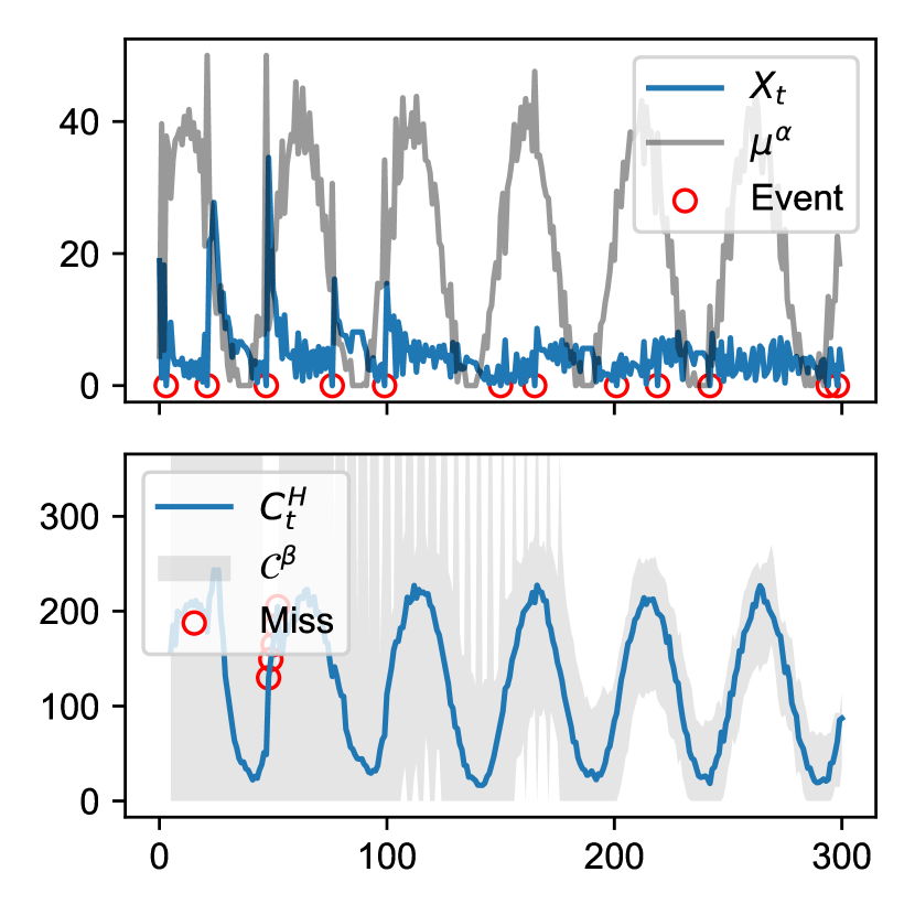
for a fixed safety stock . (If , this is also known as a ‘stockout’ event.) When (1) is not satisfied, the normal stock level is insufficient to cover demand. In this letter, we will describe an order policy that guarantees a certain service level by bounding the number of critical stock events over a specified period. At any , the policy has an operating cost, denoted , over a future time horizon of length . To forecast its costs online, we develop a method for constructing prediction intervals that will cover at a specified coverage level . Fig. 1 provides an illustrative example of the joint control and cost inference method proposed in this letter.
Notation We employ the following notation: , , .
2 Problem formulation
The stock of an inventory system follows a discrete-time dynamical equation
| (2) |
where order is placed at time instant and a demand is subsequently observed. The initial stock is . For ease of exposition and without loss of generality, we will work with , so that critical stock events are indicated by . The generalization to is straight forward.
At any , we have access to historical stock data, demand data, and side information , collected in the variable . An order policy
is the control law of interest. We define its service level as the fraction of non-critical stock events over a period . Our primary problem is to construct a policy that ensures a service level of at least , that is
| (3) |
with a user-defined rate . We call all policies that ensure (3) admissible with a service level .
Since any admissible policy can be replaced by and remain admissible, we will assume all admissible policies fulfil without loss of generality. Note that the trivial policy is also admissible but may hold a wastefully large stock beyond the specified service level. We are therefore seeking admissible policies with lower operating costs, that adapt to the information obtained about the demand process.
Let denote the operating cost of policy at time . Then its future operating cost over time horizon is
| (4) |
The choice of cost function is application dependent. One example is the cost of holding stock, e.g., . The current period cost is available in next period side information . Operating costs depends critically on the demand process , which is unknown. We therefore seek to construct prediction intervals that cover the future operating costs with a coverage level . That is,
| (5) |
where is a user-defined rate.
3 Method
Let be any predictor of the demand. Then the policy
| (6) |
is data-driven control law in which the orders are proportional to the predicted lack of stock. The demand predictor could assume any form, e.g.,
| (7) |
where is a simple autoregressive exogenous input (ARX) model. The more accurate models use, the less excess orders are made which keeps operating costs low. However, no matter how sophisticated the models are, the resulting policy (6) is not ensured to be admissible under an unknown demand process .
We will introduce integral action which takes into account the cumulative critical stock events to render (6) admissible with a service level . After deriving such an admissible order policy, we turn to the problem of inferring its future operation cost . The control and inference problems will be tackled by introducing nonlinear gain functions that bound error processes.
Our proof technique is inspired by [15], which develops a one-step-ahead method for time-series prediction. However, the cited paper does not consider interventions and their feedback effects, as is the focus of automatic control, nor the problem of providing multi-step-ahead prediction guarantees for future operating costs of a dynamic interventional policy.
3.1 Error Bound Functions
Let the integer denote an error process such that and . For instance, it may count the number of critical stock events: . We will now seek a function that can bound the error process.
Definition 1 (Error bound function)
Any nondecreasing function that satisfies .
A simple (piece-wise) linear example is
| (8) |
with parameters and . The parameter specifies an initial period in which we tolerate no errors, which leads to conservative policies. This is useful if the demand predictor requires some burn-in time. After a period , there is a linear increase of the error bound function from to . To determine a suitable integral action in a policy, we consider gain functions associated with .
Definition 2 (Associated gain)
An error function has an associated gain function if it satisfies
| (9) |
where is a saturation level.
Lemma 1
Consider any error bound function with an associated gain . If a saturated gain implies no error growth, i.e., , then the error process is bounded as
| (10) |
Proof 1
The proof is by induction. Base case holds by nonnegativity of the error bound function. Consider the inductive assumption . Two cases arise:
Case i) . Then and .
Case ii) . Then .
Finally, follows by the definition of .
Lemma 1 justifies the term ‘error bound function’ for . We will now turn to formulating a nonlinear gain function that adds integral action to the policy so as to render it admissible. The methodology will then be extended to infer the future operating costs.
3.2 Admissible policy
Theorem 2
Define the nonlinear gain
| (11) |
Then for any demand predictor , the order policy
| (12) |
is admissible with a service level (see (3)).
3.3 Valid cost inference
We now turn to forecasting the operating costs (4) of an admissible policy.
Similarly to the admissible policy construction that starts with a nominal predictor, the valid cost inference method starts with any nominal prediction interval . To make things concrete, consider nominal intervals produced by a quantile estimator. Let be a simple point predictor of the cost and define its empirical error as . Then a quantile estimator is given by:
| (17) |
and using it we can define a nominal prediction interval as
| (18) |
This nominal interval will be adjusted by introducing a gain as we show next.
Theorem 3
Assume non-negative bounded cost over a finite horizon, , where the upper bound may be infinity. Consider a horizon and any nominal prediction interval . Define an adjusted prediction interval
| (19) |
where
| (20) |
and
| (21) |
is a gain associated with the error bound function in (8) using in lieu of . Then has a coverage level according to (5).
Remark 1
A similar result holds for the special case of , but is omitted here for sake of brevity.
Remark 2
For we use as a default value and the burn-in period is problem dependent.
Proof 3
Define
| (22) |
Let the number of observed miscoverage events at time be define as that we want to bound by where . Next, define the error process to be the number of known as well as potential miscoverage events:
| (23) |
so that . Let be the saturation level. Then a direct verification shows that . We can therefore use Lemma 1 to show that . Since , we have also proven that
| (24) |
and therefore that has a coverage level .
4 Numerical experiments
The proposed order policy, and the online prediction interval for its future operational costs, are illustrated in a series of simulations using synthetic and real data. In all cases, we fix the prescribed service levels to and the coverage level to .
The operating cost is taken to be cost of purchase plus holding; for a holding cost , . A direct verification shows the finite horizon operating cost is upper bounded by . For simplicity, we use .
The nominal demand predictor used is a linear-in-parameters autoregressive model (7), where parameters are tracked by recursive least squares (RLS) [16, eq. 9.12]. To reduce the burn-in time, the RLS parameters are initialized by tracking on historical data , , recorded under an alternative policy, namely the empirical -quantile of demand; .
To construct the nominal prediction interval (18), we use another linear-in-parameters autoregressive model with parameters tracked by RLS,
This model predicts the future costs of the specific policy, and there are no data on this policy for . Therefore, no pre-training is done. The parameters are initialized with and the first element is set to , which yields a conservative initial prediction.
4.1 Synthetic data
We explore the order policy and cost inference methods on three rather different demand processes. All simulations on synthetic data use , and , and the demand is upper bounded by .
For demand prediction, we use model orders in (7), and set the RLS forgetting factor to . For cost inference, we use the feature vector of a linear AR-5 model for steps ahead prediction .
4.1.1 Periodic demand
The unknown demand process is assumed to follow
| (25) |
where and the demand is clipped to the interval . This captures seasonality with random shocks. In the cost inference, we use the RLS forgetting factor and set a burn-in time of samples. Fig. 1 shows the periodic orders resulting from the policy. We also see that the cost inference starts to become informative around .
4.1.2 Spiking demand
The unknown demand for items assumed to be proportional to the size of a latent infected population ,
which models episodic demand that arises from infectious decreases. Specifically, follows a stochastic ‘Susceptible-Infected-Removed’ or SIR-type model:
| (26) |
In (26), we have that
and . In each time step, with 3% probability, the population loses immunity and 0.1% of the population gets infected.
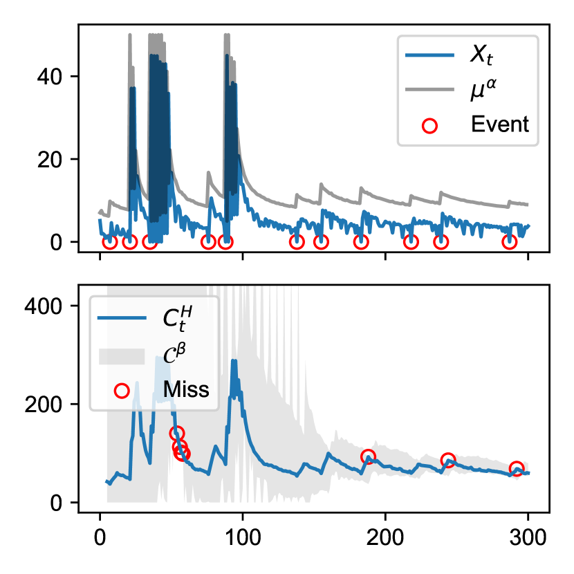
In the cost inference, we use the RLS forgetting factor and set a burn-in time of samples. Fig. 2 shows a spiking order pattern resulting from the policy. Note how the orders drop to zero during a longer period only to shoot up at the end.

4.1.3 Feedback demand
The unknown demand is assumed to depend on the stock level and therefore introduces feedback into system. Specifically, the demand process is
| (27) |
where . In the cost inference, we use and set the burn-in period to samples. Fig. 3 shows a considerable tightening of the cost inference tightens considerably after .

4.2 Electricity dataset
The previous results validate the guarantees of the order policy and cost inference methodology for rather different synthetic demand processes. As an example of a real-world demand process, we now use the electricity demand variable (NSWDemand) in the Elec2 dataset[17]. This process represents seasonality and shocks as well as other distribution shifts. It is therefore both interesting and challenging to analyze. The full dataset records the demand every 30 minutes (48 samples per day) for ca 900 days, normalized so that . We set the cost horizon to corresponding to 1 day. The pretraining window length to 3 days () and algorithm is run over 12 weeks of time periods (). The first datapoints are used for selecting suitable hyperparameters. The algorithm is then run on the subsequent samples.
Concerning hyperparameter selection, we chose demand model orders , in (7), and set the RLS with forgetting factor to . The cost inference feature map was set to include an autoregressive model of order 24 with additional Fourier coefficients representing periods of 3, 6, 12, 24 hours, and 7 days. The burn-in time was and the forgetting factor was .
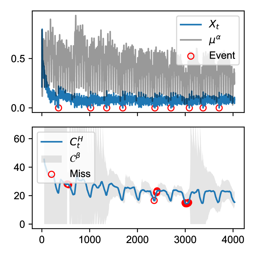
Fig. 4 shows strong periodic variations as well as sudden spikes in the orders. Despite significant variability in demand, the order policy ensures the prescribed service level . We also note that the cost inference tightens as in the previous case, but around demand fluctuations lead to several miscoverage events. These inflate the prediction intervals, which subsequently shrink again.

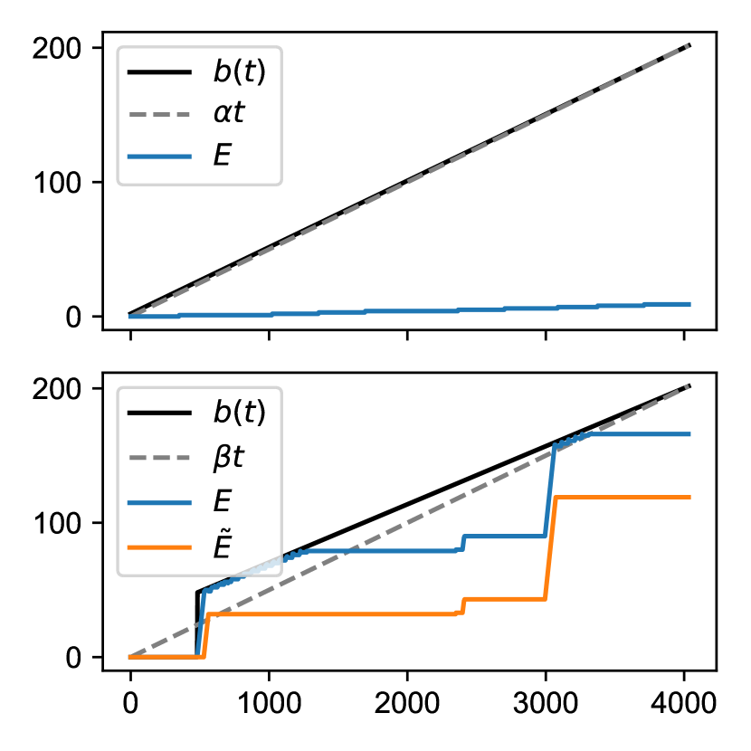
We use this example to illustrate in Fig. 5 the error processes associated with the order policy and cost inference, respectively. These processes are bounded by , which determines the associated gains.

5 Discussion
We have considered an inventory control problem with an unknown demand process in which order policies can be constructed with certified service levels and their operating cost can be forecast with a prescribed coverage level. These guarantees hold under very weak assumptions on the unknown demand process. We have verified the methods numerically and illustrated them on synthetic and real data.
The method builds on any nominal predictors of the demand and operating cost, which are adjusted using a nonlinear integration of errors made in the policy or cost inference, respectively. Several design choices are in fact possible here. In the simulation studies we used classical linear autoregressive models, but the use of more sophisticated predictors, such neural networks, is rather straightforward.
The error bound function and the associated gain function of choice affect the conservativeness of the method. In our experiments, we used the error bound function (8) with a simple parametrization, where we adjust the burn in time reflecting the fact that different models need more data to predict well. More complicated error bound functions are conceivable, which depend not only on time but also on the accuracy of the nominal predictor models.
Further exploratory work may study the impact of the choice of prediction models, as well as error bound functions and associated gains, on the operating costs and the tightness in cost inference. This may lead to finding more efficient admissible policies and cost inferences.
6 CRediT authorship contribution statement
Ludvig Hult: Conceptualization, Formal Analysis, Investigation, Software,
Dave Zachariah: Funding acquisition, Writing – review & editing, Conceptualization, Supervision
Petre Stoica: Writing – review & editing
References
- [1] K. J. Arrow, S. Karlin, H. E. Scarf, M. J. Beckmann, J. Gessford, and R. F. Muth, Studies in the mathematical theory of inventory and production, ser. Stanford mathematical studies in the social sciences. Stanford, California: Stanford university press, 1958.
- [2] S. Axsäter, Inventory Control, ser. International Series in Operations Research & Management Science. Springer International Publishing, 2015, vol. 225. [Online]. Available: https://link.springer.com/10.1007/978-3-319-15729-0
- [3] D. P. Bertsekas, Dynamic programming and stochastic control. Academic Press, 1976, vol. 125.
- [4] ——, Dynamic programming and optimal control. Athena Scientific, 1995.
- [5] A. Bensoussan, Dynamic programming and inventory control. Amsterdam: IOS Press, 2011.
- [6] A. C. Radasanu, “Inventory management, service level and safety stock,” Journal of Public Administration, Finance and Law, vol. 5, no. 9, pp. 145–153, 2016.
- [7] D. Bijulal, J. Venkateswaran, and N. Hemachandra, “Service levels, system cost and stability of production–inventory control systems,” International Journal of Production Research, vol. 49, no. 23, p. 7085–7105, dec 2011. [Online]. Available: https://doi.org/10.1080/00207543.2010.538744
- [8] G. J. Van Houtum and W. H. M. Zijm, “On the relationship between cost and service models for general inventory systems,” Statistica Neerlandica, vol. 54, no. 2, p. 127–147, 2000. [Online]. Available: https://onlinelibrary.wiley.com/doi/abs/10.1111/1467-9574.00132
- [9] C. E. Larson, L. J. Olson, and S. Sharma, “Optimal inventory policies when the demand distribution is not known,” Journal of Economic Theory, vol. 101, no. 1, p. 281–300, nov 2001. [Online]. Available: https://www.sciencedirect.com/science/article/pii/S0022053100927728
- [10] X. Yan, X. Chao, and Y. Lu, “Optimal control policies for dynamic inventory systems with service level dependent demand,” European Journal of Operational Research, vol. 314, no. 3, pp. 935–949, 2024. [Online]. Available: https://www.sciencedirect.com/science/article/pii/S0377221723008287
- [11] J. Huber, S. Müller, M. Fleischmann, and H. Stuckenschmidt, “A data-driven newsvendor problem: From data to decision,” European Journal of Operational Research, vol. 278, no. 3, p. 904–915, Nov. 2019. [Online]. Available: https://linkinghub.elsevier.com/retrieve/pii/S0377221719303807
- [12] R. Levi, G. Perakis, and J. Uichanco, “The data-driven newsvendor problem: New bounds and insights,” Operations Research, vol. 63, no. 6, p. 1294–1306, dec 2015. [Online]. Available: https://pubsonline.informs.org/doi/10.1287/opre.2015.1422
- [13] E. Saha and P. K. Ray, “Modelling and analysis of inventory management systems in healthcare: A review and reflections,” Computers & Industrial Engineering, vol. 137, p. 106051, 2019. [Online]. Available: https://www.sciencedirect.com/science/article/pii/S0360835219305108
- [14] M. Bijvank and I. F. A. Vis, “Inventory control for point-of-use locations in hospitals,” Journal of the Operational Research Society, vol. 63, no. 4, p. 497–510, Apr. 2012. [Online]. Available: https://doi.org/10.1057/jors.2011.52
- [15] A. N. Angelopoulos, E. Candes, and R. Tibshirani, “Conformal PID control for time series prediction,” in Thirty-seventh Conference on Neural Information Processing Systems, 2023. [Online]. Available: https://openreview.net/forum?id=zPYeYv6YYs
- [16] T. Söderström and P. Stoica, System identification. New York, NY: Prentice-Hall, 1989.
- [17] M. Harries, “Splice-2 comparative evaluation: Electricity pricing,” University of New South Wales, Tech. Rep. UNSW-CSE-TR-9905, July 1999.