Mobile Robot Sensory Coverage in 2-D Environments:
An Optimization Approach with Efficiency Bounds

Abstract

This paper considers three related mobile robot multi-target sensory coverage and inspection planning problems in 2-D environments. In the first problem, a mobile robot must find the shortest path to observe multiple targets with a limited range sensor in an obstacle free environment. In the second problem, the mobile robot must efficiently observe multiple targets while taking advantage of multi-target views in an obstacle free environment. The third problem considers multi-target sensory coverage in the presence of obstacles that obstruct sensor views of the targets. We show how all three problems can be formulated in a MINLP optimization framework. Because exact solutions to these problems are NP-hard, we introduce polynomial time approximation algorithms for each problem. These algorithms combine polynomial-time methods to approximate the optimal target sensing order, combined with efficient convex optimization methods that incorporate the constraints posed by the robot sensor footprint and obstacles in the environment. Importantly, we develop bounds that limit the gap between the exact and approximate solutions. Algorithms for all problems are fully implemented and illustrated with examples. Beyond the utility of our algorithms, the bounds derived in the paper contribute to the theory of optimal coverage planning algorithms.

I Introduction

In the robot sensory coverage problems considered in this paper, a mobile robot must choose its motions so that its sensors can inspect multiple targets in a bounded environment. Robot sensory coverage applications include mine sweeping [2], crop sampling [35], intruder detection [12] and sewage system inspection [29]. Other applications include aerial inspection of industrial installations [3, 5], aerial search [28], seafloor mapping [16] and ship hull inspection [15]. See surveys by Acar and Choset [1] and Galceran [17].

This paper studies three related mobile robot sensory coverage planning problems in 2-D environments. In the first two problems, a mobile robot must efficiently observe multiple targets with a limited range sensor in an obstacle free environment. First observing one target at a time, then exploiting possible multi-target views along the robot path. In the third problem, a mobile robot must efficiently observe with a limited range sensor multiple targets among stationary obstacles that obstruct sensor views of the targets.

Why do we study the multi-target sensory coverage planning problem, and why do we emphasize an optimal shortest path framework? On every day until the year 2030, the world will add $\sim$1 gigawatt of solar power generation capacity. Some solar installations will be as large as 5 miles on a side. These facilities must be inspected on a regular basis, presumably by robots. Simple boustrophedon paths will suffice to inspect the solar panel surfaces by aerial drones. But the electrical inverter modules and electrical junctions boxes, whose failure can be detected by thermal cameras, are irregularly sited inspection targets. The vast size of these inspection problems requires a shortest path strategy.

One of the novelties of this paper is to formulate these problems in a rigorous optimization framework. This framework brings the computational difficulty of coverage to the forefront. We show that all problems can be posed as mixed integer nonlinear optimization problems (MINLP). Because these MINLPs are NP-hard, we introduce polynomial time algorithms to approximately solve these problems. In addition to new algorithms, we provide rigorous efficiency bounds on the mobile robot path length that set new upper bounds on the length of a robot path to solve an inspection problem. These are the paper’s two main conceptual contributions.

The MINLP approach and our approximate solution methods provide a flexible framework for coverage planning that can be extended to target specific observation requirements, different sensor scanning patterns, terrain dependent travel cost and control input limits. Prior works have often made restricted choices of these parameters

Related work: We are not the first to recognize that sensory coverage planning (which is NP-hard) can be solved under MINLP formulation. Gentilini [18] adapted the MINLP formulations of Current  [11] and Golden [19] to plan the motion of a robot arm to inspect 3-D objects with a distal camera. The camera visits viewing neighborhoods specified as convex sets. A direct optimization of the viewing path was proposed. However, direct MINLP solvers can only find globally optimal solutions in reasonable computation times for small numbers of regions [4, 7, 27]. Large number of targets can be solved using branch and bound methods, with much longer computation time [10].

This paper solves off-line sensory coverage planning  problems using a two-stage approach that is related to a long tradition in robotics. Danner [12] uses a two-stage scheme to plan mobile robot intruder detection routes in 2-D environments. The first stage samples candidate robot sensing locations. The second stage computes in polynomial time a tour that visits the selected sensing locations.

Englot [14] used a two-stage scheme for underwater inspection of ship hulls. A mesh representation of the hull defines a collection of targets to observe. The first stage uses random sampling to construct a graph that connects sensing nodes with multiple target views. The second stage  computes a tour through the sensing nodes. Bircher [5] also used a two-stage scheme to plan aerial inspection of industrial sites. Mesh-based facets of the environment form the collection of targets to observe. Initial sensor node locations are chosen according to the sensor viewing pattern. The first stage computes a tour that visits all sensing nodes. The second stage adjusts the sensing positions to reduce the robot path length. This process repeats several times, but efficiency bounds on the coverage path length are not discussed.

The MINLP formulation has been applied to a different problem of computing collision free paths for robot arms [30]. The robot arm joint space is partitioned into collision free convex cells whose visitation order is represented by the MINLP integer variables. The integer variables are then relaxed into continuous variables and the MINLP is solved as a convex optimization problem having only continuous variables. However, the solution needs rounding back into integer variables in a manner that does not guarantee efficiency bounds on the solution path.

The mobile robot sensory coverage problem studied in this paper is related to the Traveling Salesperson Problem (TSP) with neighborhoods [31] in computational geometry. This NP-hard problem is approximately solved in polynomial time by finding a tour that visits each neighborhood, and then bounding the length of this tour in terms of the optimal tour length through the specified neighborhoods.

In this paper, the neighborhoods represent sensing regions modeled as circles centered at the targets. When the circles have equal size and do not overlap, Dumitrescu [13] computes in polynomial time a tour that visits each circle with path length $l(path)\!\leq\!(\mbox{\small$1$}\!+\!\tfrac{8}{\pi})(\mbox{\small$1$}\!+\!\epsilon)\!\cdot\!l_{opt}$, where $l_{opt}$ is the optimal tour length. The $\mbox{\small$1$}\!+\!\epsilon$ coefficient represents an approximation of an initial TSP tour that passes through the circle centers. For instance, $\mbox{\small$1$}\!+\!\epsilon\!=\!\tfrac{3}{2}$ when Christofides [9] is used to approximate the TSP tour. When the sensing circles possibly overlap, Dumitrescu [13] computes a tour that visits each circle with path length bound $l(path)\!\leq\!\pi(\mbox{\small$1$}\!+\!\tfrac{8}{\pi})(\mbox{\small$1$}\!+\!\epsilon)\!\cdot\!l_{opt}$, where $l_{opt}$ is the optimal tour length.

Isler adapted these techniques to sample crop data from circular areas (with path length efficiency bound [35]), and then to aerial robot inspection of ground targets visible through vertical cones of variable heights with path length efficiency bound [32].

Paper contributions and format: In the sensory coverage problems considered in this paper, the mobile robot starts at the first target location $T_{1}$, moves to observe intermediate targets $T_{2},\ldots,T_{n-1}$ in any order, then stops within the detection range of a final target $T_{n}$. This problem is termed $S$-to-$T$ sensory coverage, where $S\!=\!T_{1}$ and $T\!=\!T_{n}$. The mobile robot observes the targets at discrete sensing locations along its path while ensuring that the targets lie within the detection range $r$ of its on-board coverage sensors. The robot sensing locations thus lie in circular sensing regions of radius $r$ centered at the targets (Fig. 1).

The paper first describes the MINLP formulation of multi-target coverage in obstacle free environments with non-overlapping sensing regions. An approximate shortest sensory coverage path is computed in two stages. First, a polynomial time algorithm finds a bounded approximation to the optimal $S$-to-$T$ sensory coverage path, which establishes the sensing node visitation order. The sensing nodes positions are then optimized for the shortest path using efficient convex optimization. The robot’s path length bound is shown to approach $l(path)\!\leq\!\tfrac{10}{3}\!\cdot\!l_{opt}$, where $l_{opt}$ is the optimal $S$-to-$T$ sensory coverage path length. The approximation coefficient improves on [13] and is shown to be tight.

The paper next develops a novel MINLP formulation for multi-target sensory coverage when the sensing regions may overlap in an obstacle free environment. A modified two-stage approximation algorithm first places sensing nodes on the perimeter of base set sensing circles that overlap all other sensing circles. Application of the algorithm described above (approximate path construction, followed by sensing location optimization) is followed by a process of sensing node reduction. The constructed path satisfies the bound $l(path)\!\leq\!\frac{5}{3}\cdot 9\cdot l_{opt}$ (with some constants neglected), where $l_{opt}$ is the length of the shortest path that observes all targets while taking advantage of multi-target views. The approximation bound improves on [13] but is not a tight bound.

Figure 1: The problem geometry showing circular sensing regions centered at the targets and typical robot sensor footprints with detection range $r$.

The third sensory coverage problem includes polygonal obstacles in the environment. The targets can only be viewed from obstacle bounded viewing regions of maximal detection range $r$. The sensory coverage path among obstacles can still be computed by a polynomial time two-stage approach. Path length optimization occurs within the obstacle free space, and the number of sensing is reduced, when possible. The path length approximation bound for this problem uses two parameters. The number of obstacle vertices within detection range of the targets, $m$, and the circular radius representing the average area of the viewing regions, $\bar{\rho}\!\leq\!r$. The sensory coverage path satisfies the bound $l(path)\!\leq\!\frac{5}{3}(\mbox{\small$1$}\!+\!\mbox{\small$8$}\frac{r^{2}}{\bar{\rho}^{2}})\cdot(l_{opt}+2r\!\cdot\!m)$ (with some constants neglected), where $l_{opt}$ is the length of the optimal $S$-to-$T$ sensory coverage path in the environment. All algorithms are fully implemented and illustrated with execution examples.

A very preliminary version of this work appeared in [8]. The present paper sharpens Proposition 2 and provides the missing proof of this proposition. The bulk of Section IV on sensor node reduction is entirely new. Moreover, all of Section V and its novel bounds are new material.

The paper is structured as follows. Section II formulates the first multi-target sensory coverage problem as a MINLP problem. Section III describes a two-step approximation algorithm for this problem and develops a path length approximation bound. Section IV adds multi-target views to the MINLP formulation, then describes an analogous approximation algorithm, a sensing node reduction algorithm, and a path length approximation bound. Section V generalizes the MINLP formulation to multi-target sensory coverage in the presence of obstacles. The section describes an approximation algorithm, followed by analysis of the algorithm’s path length approximation bound. The conclusion discusses an extension of the MINLP approach to partially known environments and 3-D sensory coverage planning problems.

II MINLP Formulation of the Multi-Target Sensory Coverage Problem

This section describes the MINLP formulation of the basic multi-target sensory coverage problem. The mobile robot moves in a 2-D environment free of obstacles using an ideal position sensor and a finite detection range coverage sensor, whose footprint forms a circular or convex sector with detection range $r$ (Fig. 1). The robot must observe targets $T_{1},\ldots,T_{n}$ from discrete sensing nodes $S_{1},\ldots,S_{n_{s}}$ ($n_{s}\!\leq\!n$) along its path. The robot starts at target $T_{1}$ (which is also labeled as sensing node $S_{1}$) and ends within detection range of $T_{n}$, but otherwise observes the intermediate targets $T_{2},\ldots,T_{n-1}$ in any order. The sensing region that surrounds each target, $R(T_{i})$, is the circle of radius $r$ centered at $T_{i}$ (Fig. 1). This is a specific type of viewing region, $V(T_{i})$, which describes the area from which target $T_{i}$ can be observed. When the robot sensor is located in $R(T_{i})$, there exist sensor viewing directions that can observe target $T_{i}$.

The multi-target sensory coverage problem: The simplest problem assumes one sensing node per target, $n_{s}\!=\!n$, in an obstacle free environment. The goal is to find the shortest path, $\mathcal{P}$, that allows the robot to observe all targets $T_{1},\ldots,T_{n}$ from sensing nodes $S_{1},\ldots,S_{n}$, such that $S_{1}\!=\!T_{1}$ and $S_{n}\!\in\!R(T_{n})$.

The path $\mathcal{P}$ is chosen to minimize the cost

$$Cost(\{S_{1},\ldots,S_{n}\},\{\xi_{ij}\})=\ \sum_{i=1}^{n}\sum_{j=1,j\neq i}^{n}\!\xi_{ij}\!\cdot\!d(S_{i},S_{j})$$ (1)

over the sensing node locations $S_{1},\ldots,S_{n}\in\mbox{$I\!\!R$}^{2}$ ($S_{1}\!=\!T_{1}$) and incidence variables, $\xi_{ij}$ for $i,j\in\{1,\ldots,n\}$, such that

$$\xi_{ij}=\begin{cases}1&\mbox{\rm$T_{j}$ is observed immediately after $T_{i}$ is observed}\\ 0&{\rm otherwise}\end{cases}$$

with $d(S_{i},S_{j})\!\geq\!0$ denoting the distance between sensor nodes $S_{i}$ and $S_{j}$. Terrain dependent travel costs can be handled by non-symmetric travel costs. This paper assumes symmetric travel costs, $d(S_{i},S_{j})\!=\!d(S_{i},S_{j})$. In the symmetric case it suffices to use the reduced indices $j\!>\!i$ in Eq. (1).

For the sensory coverage path to be well defined, the cost minimization must satisfy the following constraints.

1. Full path constraints: The path $\mathcal{P}$ must pass through each sensing node

   $$\sum_{j=2}^{n}\xi_{1j}=1,\quad\quad\sum_{i=1}^{n-1}\ \xi_{in}=1,\vspace{-.13in}$$ (2)

   and

   $$\sum_{j=1}^{i-1}\xi_{ji}+\sum_{j=i+1}^{n}\ \xi_{ij}=2\hskip 10.00002pt\mbox{\hskip 15.00002pt $i=2\ldots n\!-\!1$.}\vspace{-.08in}$$ (3)

   Eq. (2) ensures that a single edge of $\mathcal{P}$ exits $S_{1}$ and a single edge enters $S_{n}$. Eq. (3) ensures that a single edge of $\mathcal{P}$ enters (first summand) and a single edge exits (second summand) each intermediate sensing node.

2. Connected path constraints: Additional constraints are needed to ensure that $\mathcal{P}$ forms a connected path. Let $\mathcal{S}\!=\!\{S_{1},\ldots,S_{n}\}$ be the set of sensing nodes. Let $W$ be the index set of three or more distinct sensing nodes, and let $|W|$ denote the set size. The constraints

   $$\sum_{i\in W,j\in W}\!\xi_{ij}\leq|W|\!-\!1,\ \forall W\subseteq\mathcal{S}\!-\!\mbox{\small$\{S_{1},S_{n}\}$},|W|\geq 3$$

   prevent disconnected sub-paths by preventing sets of $|W|\!\geq\!3$ sensing nodes from forming disjoint loops (Fig. 2). The number of such constraints

   $$\sum_{k=3}^{n-1}{{n\!-\!2}\choose k}=2^{n-1}\!-\!\frac{1}{2}(n\!-\!1)(n\!-\!2)-1$$

   is exponential in $n$, which highlights the NP-hardness of the multi-target sensory coverage problem.

3. Sensing region constraints: Each sensing node $S_{i}$ must lie inside the circular sensing region $R(T_{i})$, expressed by the quadratic constraint

   $$||S_{i}-T_{i}||^{2}\ \leq\ r^{2}\hskip 10.00002pt\mbox{\hskip 10.00002pt $S_{i}\in\mbox{$I\!\!R$}^{2}$, \ $i=1\ldots n$.}$$ (4)

Figure 2: A non-valid sensory coverage path starts at $S_{1}\!=\!T_{1}$ and ends at $S_{9}\!\in\!R(T_{9})$. The disjoint loop through the sensing nodes $W\!=\!\{S_{5},S_{6},S_{7},S_{8}\}$ does not satisfy the constraint $\sum_{i\in W,j\in W}\xi_{ij}$$\!\leq\!3$.

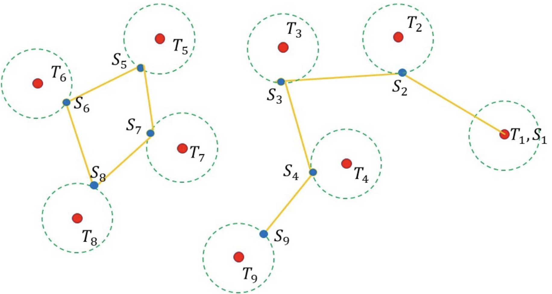
Problem $\#1$: Compute the minimum cost $S$-to-$T$ path $\mathcal{P}$ that visits variable sensing nodes $S_{1},\ldots,S_{n}$ such that all targets $T_{1},\ldots,T_{n}$ are observed at the sensing nodes. This problem is formulated as the MINLP optimization problem

$$(\mathcal{S}^{*},\{\xi^{*}_{ij}\})=\operatorname*{Arg\,Min}_{\mathcal{S},\{\xi_{ij}\}}\bigg{(}\sum_{i=1}^{n}\sum_{j=i,j>i}^{n}\xi_{ij}\!\cdot\!d(S_{i},S_{j})\bigg{)}$$

where $d(S_{i},S_{j})\!=\!\mbox{\small$\mbox{$\|S_{i}\!-\!S_{j}\|$}$}$ is the Euclidean distance. The sensing nodes $\mathcal{S}\!=\!\{S_{1},\ldots,S_{n}\}$ and the incidence variables $\{\xi_{ij}\}$ are subject to the constraints

$$\sum_{j=2}^{n}\xi_{1j}=1,\quad\quad\sum_{i=1}^{n-1}\ \xi_{in}=1$$ (5)

$$\sum_{j=1}^{i-1}\xi_{ji}+\sum_{j=i+1}^{n}\ \xi_{ij}=2\hskip 10.00002pt\mbox{\hskip 15.00002pt $i=2\ldots n\!-\!1$}$$ (6)

$$\!\!\sum_{i\in W,j\in W}\!\!\!\xi_{ij}\!\leq\!|W|\!-\!1,\ \forall W\subseteq\mathcal{S}\!-\!\mbox{\small$\{S_{1},S_{n}\}$},|W|\!\geq\!3\ \ \$$ (7)

$$\xi_{ij}\in\{0,1\}\hskip 15.00002pt\hskip 10.00002pt\mbox{\hskip 15.00002pt $1\leq i,j\leq n$}$$ (8)

$$S_{i}\ \in R(T_{i})\hskip 10.00002pt\mbox{\hskip 27.50003pt $S_{i}\in\mbox{$I\!\!R$}^{2}$, \ $i=1\ldots n$}$$ (9)

where the sensing range constraints take the quadratic form of Eq. (4). A convex polyhedral sensing pattern can alternatively included by a set of linear constraints. Generically, for any convex sensing footprint, these constraints are simply $S_{i}\in V(T_{i})$.

Figure 3: MINLP solution using BONMIN for eight targets that lie at the centers of the red sensing circles. (a) Initial path guess, and (b) the optimal sensory coverage path where each sensing node (blue dots) lies in a target centered sensing circle. (c) Another initial path guess with different visitation order for $T_{8}$, and (d) the MINLP solution gives the same globally optimal path.

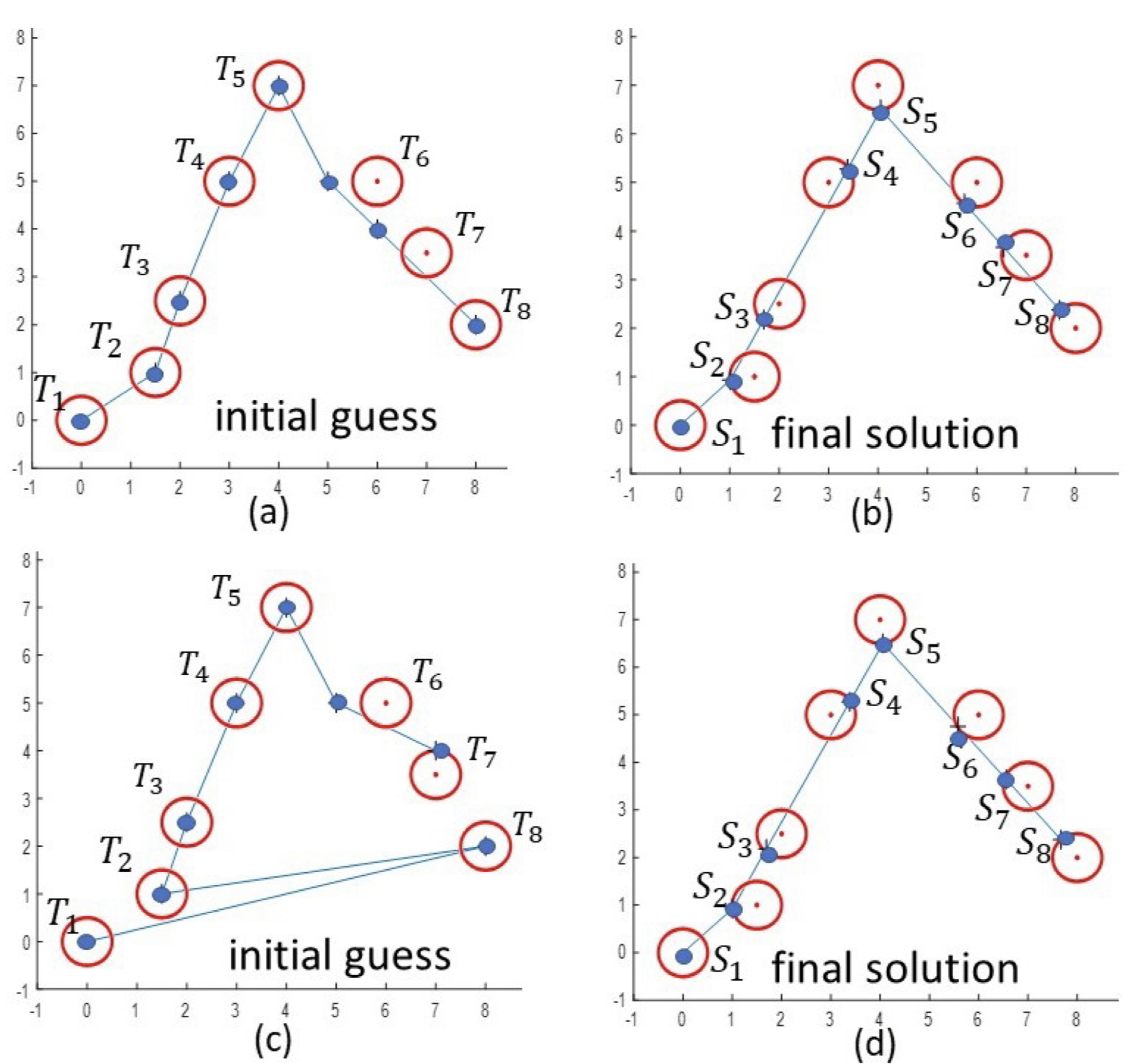
Exact MINLP example: Since Problem $\#1$ is NP-hard, direct MINLP solvers can only solve simple instances in practical computation time. The example in Fig. 3 uses BONMIN  [7], a branch-and-bound solver with nonlinear trust region that computes globally optimal solutions. BONMIN requires an initial, but not necessarily feasible, sensing nodes path guess (Fig. 3(a)). The optimal solution in Fig. 3(b) was computed in 5.8 seconds. Another initial path with different visitation order (Fig. 3(c)) gives the same optimal solution (Fig. 3(d)), in roughly the same computation time.  $\circ$

III Multi-Target Sensory Coverage with Path Length Bound

This section describes a two-stage polynomial time algorithm that approximatly solves Problem $\#1$, then provides a bound on the worst case path length produced by the algorithm. Hoogeven’s algorithm [22] is first used to determine the sensing nodes visitation order. The Hoogeveen path solution assigns fixed values to the incidence variables, thereby approximating a solution of the S-T TSP problem on the targets. Then, initial sensing node locations are placed at the target locations. Next, convex optimization finds the sensing node locations that yield the shortest sensory coverage path, given the visitation order. The section then analyzes this algorithm’s path length approximation bound.

Hoogeveen $S$-to-$T$ shortest path approximation: Hoogeveen’s algorithm [22], summarized in Algorithm  1, generates in polynomial time a path that visits all sensing nodes, which are initialized to the target locations, with a path length approximation bound that is described below. The algorithm first computes in line  2 a complete graph, $G$, by joining every pair of sensing nodes $S_{i}$ and $S_{j}$ with edge weight $d(S_{i},S_{j})\!=\!\mbox{$\|S_{i}\!-\!S_{j}\|$}$. This computation takes $O(n^{2})$ time where $n$ is the total number of sensing nodes (one per target). The shortest $S$-to-$T$ path that visits all sensing nodes lies in $G$, though it is NP-hard to find this path [22].

Algorithm 1 Hoogeveen S-to-T Path Approximation

Input: Initial Sensing node locations $\mathcal{S}=\{S_{1},\ldots,S_{n}\}$

1:procedure Hoogeveen($\mathcal{S}$)

2:    $G\ =\ {\rm CompleteWeightedGraph}(\mathcal{S})$

3:    $T_{min}\ =\ {\rm MinSpanningTree}(G)$

4:    $V_{join}\ =\ {\rm WrongNodeDegree}(T_{min})$

5:    $M_{opt}\ =\ {\rm MinPerfectMatching}(V_{join})$

6:    $\mathcal{P}_{E}\ =\ {\rm EulerianPath}(M_{opt}\!+\!T_{min})$

7:    $Return({\rm Shortcut}(\mathcal{P}_{E}))$

8:end procedure

Hoogeveen’s algorithm computes in line 3 a minimum spanning tree, $T_{min}$, that spans all nodes of $G$ with minimum total edge cost. This stage is computed with Prim’s algorithm in $O(n\log n)$ time. The minimum spanning tree is augmented with edges that ensure odd degree of nodes $S_{1}$ and $S_{n}$ and even degree of all other nodes. This stage is performed in Line 4, where nodes $S_{1}$ and $S_{n}$ have wrong degree when their node degree is even in $T_{min}$, all other nodes have wrong degree when their degree is odd in $T_{min}$. The set of wrong degree nodes, $V_{join}$, is computed in $O(n)$ time and always contains an even number of nodes. In line 5, the edges to be added to $T_{min}$ are computed as a minimum perfect matching over the nodes of $V_{join}$, using Blossom’s algorithm [26] in $O(n^{3})$ time. The pairwise matchings of the nodes in $V_{join}$ forms the set of edges, $M_{opt}$, that are added to $T_{min}$ in line 6.

The larger graph, $T_{min}\!+\!M_{opt}$, is next used to compute the desired path. An $S$-to-$T$ path that traverses every edge of the latter graph exactly once (nodes may be revisited) forms an Eulerian path. The graph $T_{min}\!+\!M_{opt}$ possesses an Eulerian $S_{1}$-to-$S_{n}$ path iff $S_{1}$ and $S_{n}$ have odd degree while all other nodes have even degree. The latter graph is constructed in a manner that ensures this property, and line 6 computes in $O(n)$ time an Eulerian $S_{1}$-to-$S_{n}$ path. The Eulerian path is finally shortened in line 7 into a path from $S_{1}$ to $S_{n}$ that visits a new sensing node in each step, by taking shortcuts along the graph $G$ in $O(n^{2})$ time. Hoogeveen  [22] established that the resulting path visits every sensing node, starting at $S_{1}$ and ending at $S_{n}$, with path length bound

$$l(path)\!\leq\!l(T_{min})\!+\!l(M_{opt})\leq l_{TSP}+\tfrac{2}{3}l_{TSP}=\tfrac{5}{3}l_{TSP}$$

where $l_{TSP}$ is the length of the shortest path from $S_{1}$ to $S_{n}$ that visits all sensing nodes located at the targets.

Efficient optimization of sensing node locations: Algorithm 1 computes a sensory coverage path that does not optimize the sensing node locations. When the targets are sparsely located with non-overlapping sensing circles (overlapping sensing circles are considered in Problem #2), the sensing nodes visitation order found by Algorithm 1 is a good initial path for the next step that optimizes the sensing locations. The path computed by Algorithm  1 fixes the incidence variables, $\xi_{ij}$, thus reducing the MINLP optimization cost to a function only of the sensing node locations, $S_{1},\ldots,S_{n}\!\in\!\mbox{$I\!\!R$}^{2}$:

$$Cost(S_{1},\ldots,S_{n})\ =\ \sum_{j=1}^{n-1}\mbox{$\|S_{j+1}-S_{j}\|$}.\vspace{-.08in}$$ (10)

Each term $||S_{j+1}\!-\!S_{j}||$ is a convex function, since it is the composition of a convex norm function with the linear function $S_{j+1}\!-\!S_{j}$. The sum of convex functions is a convex function, hence the cost (16) is a convex function of $S_{1},\ldots,S_{n}$. The sensing circles form convex sets for the individual sensing node locations. Their conjunction therefore forms a convex set in the composite space $S_{1},\ldots,S_{n}$. Computation of the shortest sensory coverage path under fixed sensing node visitation order thus forms a convex optimization problem, which is summarized as Algorithm 2 and computationally solved using [20],[21].

Algorithm 2 Shortest Cover

Input: Targets $\mathcal{T}=\{T_{1},\ldots,T_{n}\}$

1:procedure ShortestCover($\mathcal{T}$)

2:    Set  $S_{i}=T_{i}$  for  $i=1\ldots n$,  $\mathcal{S}=\{S_{1},\ldots,S_{n}\}$

3:    $\mathcal{P}_{order}\ =\ {\rm Hoogeveen}(\mathcal{S})$

4:    $\{\xi_{ij}\}\ =\ {\rm Incidence}(P_{order})$

5:    $\mathcal{S}_{opt}=\operatorname*{Arg\,Min}{\rm Cost}(\{\xi_{ij}\},\mathcal{S},\mathcal{T})$

6:    $\quad\quad{\rm subject\ to}\ S_{1}=T_{1}\ {\rm and}\ S_{i}\!\in\!R(T_{i})\ {\rm for}\ i=2\ldots n$

7:    $Return({\rm path}\ \mathcal{P},\ {\rm sensing\ nodes}\ \mathcal{S}_{opt})$

8:end procedure

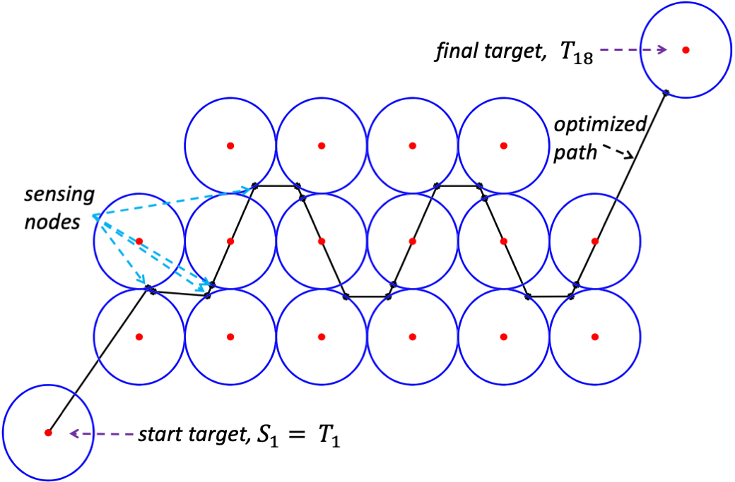
Examples: Algorithm 2 requires an initial coverage path, provided by the Hoogeveen path computed in line 3, to perform convex optimization in line 5. When Algorithm 2 is applied to the problem of Fig. 3, it yields the same optimal path as BONMIN in $0.1$ seconds (versus 5.8 seconds required by BONMIN). Algorithm 2 is next applied to the $18$ targets placed at integer locations shown in Fig. 4, with sensing circles of detection range $r\!=\!0.49$ units (the BONMIN solver was not able to solve this problem in reasonable time). Algorithm 2 computed a sensory coverage path for these targets in $0.575$ seconds, with the optimized sensing nodes (blue dots) and the coverage path (black curve) shown in Fig. 4.  $\circ$

Figure 4: Optimized sensory coverage path computed by Algorithm 2 for $18$ targets surrounded by sensing circles whose radii equal the robot detection range, $r=0.49$. The sensory coverage path is the black curve while the $18$ blue dots indicate the optimized sensing node locations.

Path length approximation bound: The approximation bound of Algorithm 2 is defined as the largest ratio of the algorithm’s path length measured relative to the optimal path length, taken over all problem instances. Our approximation bound is based on the following lemma.

Lemma 1 ([22])

Algorithm 1 computes in $O(n^{3})$ time a path that visits all initial sensing nodes. Its length satisfies $l(Alg.~{}\ref{alg:hoogeveen})\ \leq\ \tfrac{5}{3}l_{TSP}$, where $l_{TSP}$ is the length of the shortest $S$-to-$T$ path that visits all sensing nodes.

The next proposition describes the path length approximation bound for Algorithm 2.

Proposition 2

Algorithm 2 computes in $O(n^{3})$ time a sensory coverage path whose length satisfies the approximation bound

$$l(Alg.~{}\ref{alg:s_t_heuristic})\ \leq\ \tfrac{10}{3}\mbox{\small$(1\!+\!\delta(n)$})\cdot l_{opt}\vspace{-.08in}$$ (11)

where $\delta(n)\!\ll\!1$ for large $n$, $\delta(n)\rightarrow 0$ as $n\rightarrow\infty$, and $l_{opt}$ is the optimal $S$-to-$T$ sensory coverage path in the obstacle free environment.

Proof: Line 3 of Algorithm 2 computes in $O(n^{3})$ time an initial sensory coverage path for the convex optimization procedure. The complexity of Algorithm 2 therefore depends upon the relative complexity of the convex optimization procedure. When convex optimization is performed with interior point methods [6], an optimal solution is computed within $\epsilon$ accuracy in $kn^{2}\!\cdot\!\log(1/\epsilon)$ steps, where $n$ is the number of optimization variables and $k$ is the number of steps required to evaluate the cost and constraints, which is $O(n)$ in the MINLP formulation of Section II. Algorithm  2 thus takes $O(n^{3}\!\cdot\!\log(1/\epsilon))$ time.

Figure 5: Geometry of a worst case ratio of path length through the targets, $l_{TSP}$, to the optimal sensory coverage path length $l_{opt}$ (see appendix).

By Lemma 1, the initial sensory coverage path satisfies the bound $l(Alg.~{}\ref{alg:hoogeveen})\!\leq\!\tfrac{5}{3}l_{TSP}$. Algorithm 2 starts with this path, then computes a shorter path that visits optimized sensing nodes locations. Hence

$$l(Alg.~{}\ref{alg:s_t_heuristic})\leq\tfrac{5}{3}l_{TSP}\vspace{-.09in}$$ (12)

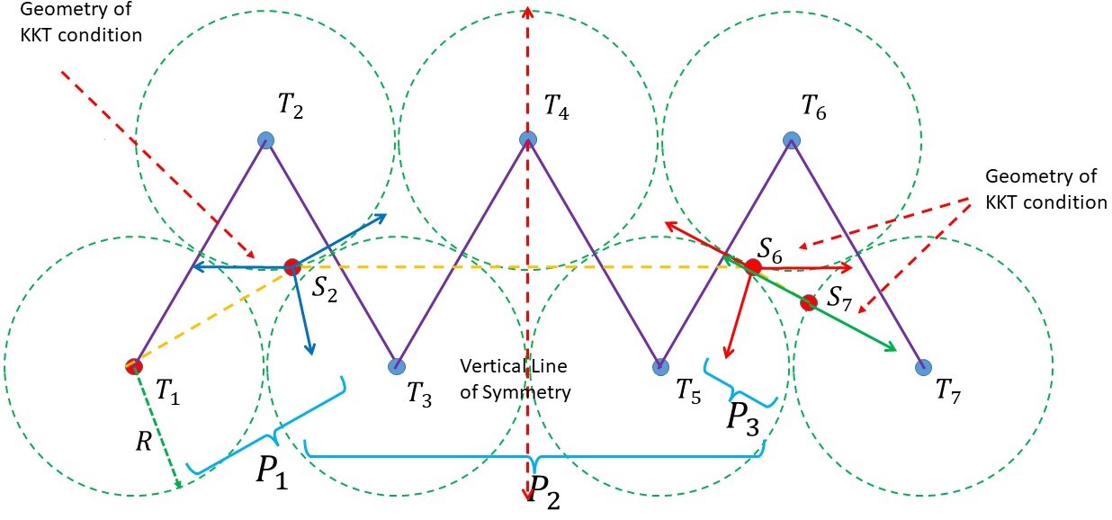
where $l_{TSP}$ is the length of the shortest $S_{1}$-to-$S_{n}$ path through sensing nodes located at the targets. As shown in Fig. 5, the geometry that leads to the worst case ratio between $l_{TSP}$ and $l_{opt}$ occurs when the sensing circle are packed in alternating linear pattern (see appendix). In this packing, the length of the shortest $S_{1}$-to-$S_{n}$ path through the targets is

$$l_{TSP}\!=\!2(n-1)r$$

while the length of the shortest sensory coverage path is

$$l_{opt}=(n-4+\kappa^{\prime}_{o})r\hskip 10.00002pt\mbox{\hskip 10.00002pt $n>4$.}$$

where $\kappa^{\prime}_{o}$ is from Eq. (27) and (25) in the appendix. It follows that the ratio $l_{TSP}/l_{opt}$ is bounded by

$$\frac{l_{TSP}}{l_{opt}}\leq\frac{2(n-1)}{n-4+\kappa^{\prime}_{o}}\hskip 10.00002pt\mbox{\hskip 10.00002pt $n>4$.}$$

Substituting for $l_{TSP}/l_{opt}$ in Eq. (12) gives

$$l(Alg.~{}\ref{alg:s_t_heuristic})\leq\frac{10}{3}\cdot\frac{n\!-\!1}{n-4+\kappa^{\prime}_{o}}\cdot l_{opt}\hskip 10.00002pt\mbox{\hskip 10.00002pt $n\geq 4$.}$$ (13)

The term that multiplies $10/3$ in Eq. (13) can be written as

$$\frac{n\!-\!1}{n\!-\!4\!+\!\kappa^{\prime}_{o}}\!=\!1\!+\!\delta(n)\hskip 6.99997pt\mbox{where}\hskip 6.99997pt\delta(n)\!=\!\frac{4\!-\!\kappa^{\prime}_{o}}{n\!-\!4\!+\!\kappa^{\prime}_{o}}.$$

Note that as $n\to\infty$, $\delta(n)\to 0$.  $\square$

IV Fewer Sensing Nodes than Targets

When the targets are located close together  in  an  obstacle-free environment, the covering robot might be able to take advantage of opportunities to view multiple targets from a single sensing location. Multi-target view opportunities can simplify and shorten the sensory coverage path. This section formulates the MINLP optimization problem that allows multi-target views, then describes a polynomial time approximation algorithm, followed by sensing node reduction along the coverage path. The section concludes with analysis of the algorithm’s path length approximation bound.

Figure 6: (a) An $18$ target (red dots) coverage problem overlaid with a dashed red circle showing the robot sensing range. (a) The $S$-to-$T$ Hoogeveen path computed by Alg. 1. (b) The optimized sensing node locations computed by Alg. 2 (blue dots). (c) When redundant sensing nodes are removed, six sensing nodes can observe all targets.

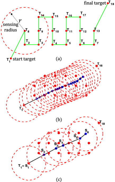
Motivational example: Fig. 6(a) shows the $18$ target example of Fig. 4, now with a larger sensing radius of $r\!=\!1.75$ units which allows individual sensing nodes to cover multiple targets. The initial Hoogeven path computed by Alg. 1 is shown in Fig. 6(a), while the optimized sensing node locations computed by Alg.  2 are shown in Fig. 6(b). The optimized sensing nodes are arranged along a nearly straight path, which is clearly the shortest path that observes all targets. When the optimized coverage path takes advantage of multi-target views, Fig. 6(c) shows that six sensing nodes suffice to observe all targets. This example shows that path optimization can be performed under maximally flexible sensing node placement, followed by sensing node pruning, or reduction, along the optimized coverage path.  $\circ$

MINLP formulation: Let $n_{s}\!\leq\!n$ denote the number of sensing nodes that now becomes an additional optimization variable. To allow fewer sensing nodes than targets, for each target $T_{i}$ the sensing constraints of Eq. (4) must be satisfied by at least one sensing node $S_{j}$ ($j\!=\!1\ldots n_{s}$). This constraint can be expressed in disjunctive form

$$\mbox{ $\bigvee$}_{j=1}^{n_{s}}\big{(}||S_{j}\!-\!T_{i}||^{2}-r^{2}\leq 0\big{)}\hskip 10.00002pt\mbox{\hskip 5.0pt $i=1\ldots n$.}\vspace{-.06in}$$

The disjunctive constraints can be expressed as a set of mixed integer constraints using viewing variables, $\eta_{ij}\!\in\!\{0,1\}$, and Big-M constants $M_{i}$ for $i\!=\!1\ldots n$ [36]. Each constant $M_{i}$ is chosen sufficiently large according to the rule

$$M_{i}\geq\max_{x\in R(T_{j}),\,j=1\ldots n}\big{\{}||x-\mbox{\small$T$}_{i}||^{2}\big{\}}\hskip 10.00002pt\mbox{\hskip 10.00002pt $i\!=\!1\ldots n$}$$ (14)

where $R(T_{j})$ is the sensing circle of radius $r$ centered at $T_{j}$. Using the Big-M constants, each target $T_{i}$ for $i\!=\!1\ldots n$ must be observed according to the conjunctive constraints

$$||S_{j}-T_{i}||^{2}\,\leq\,{\color[rgb]{0,0,0}\eta_{ij}}\!\cdot\!r^{2}+(1\!-\!\eta_{ij})\cdot M_{i}\hskip 10.00002pt\mbox{$j=1\ldots n_{s}$}$$

$$\sum_{j=1}^{n_{s}}\ \eta_{ij}\geq 1$$ (15)

$$\eta_{ij}\!\in\!\{0,1\}\hskip 10.00002pt\mbox{\hskip 10.00002pt $j=1\ldots n_{s}$.}$$

The viewing variables indicate sensing relationships: $\eta_{ij}\!=\!1$ when $S_{j}\!\in\!R(T_{i})$  and  $\eta_{ij}\!=\!0$  otherwise. Eq. (15) ensures  that at least one sensing node observes each target, with multi-views of the same target allowed. To our knowledge, this formulation represents the first complete statement of the multi-view problem with variable number of sensing nodes.

Problem $\#2$: Compute the shortest $S$-to-$T$ path $\mathcal{P}$ that visits $n_{s}\leq n$ variable position sensing nodes such that all targets $T_{1},\ldots,T_{n}$ are observed at the sensing nodes. This problem is formulated as the MINLP optimization problem

$$(n^{*}_{s},\mathcal{S}^{*},\{\xi_{ij}^{*}\},\{\eta_{ij}^{*}\})\!=\!\operatorname*{Arg\,Min}_{n_{s},\mathcal{S},\{\xi_{ij}\},\{\eta_{ij}\}}\ \!\!\bigg{(}\!\sum_{j=i,j>i}^{n_{s}}\!\!\xi_{ij}\cdot d(S_{i},S_{j})\!\bigg{)}$$

where $d(\mbox{\small$S$}_{i},\mbox{\small$S$}_{j})\!=\!\mbox{\small$\mbox{$\|S_{i}\!-\!S_{j}\|$}$}$ is the Euclidean distance. The sensing nodes, $\mathcal{S}\!=\!\{S_{1},\ldots,S_{n_{s}}\}$, and incidence variables, $\xi_{ij}$, are subject to the constraints of Eqs (5)-(8) while the sensing nodes and viewing variables, $\eta_{ij}$, must satisfy for each target $T_{i}$ ($i\!=\!1\ldots n$) the multi-view constraints (15).

Figure 7: A $24$ targets example with overlapping sensing circles. The base set circle indices are $\mathcal{I}\!=\!\{2,6,7,8,12,13,14,15,18,24\}$ (blue circles). Initial sensing nodes selected on the perimeter or center of the base set circles (blue dots).

Polynomial time algorithm for multi-target views: The algorithm that approximately solves Problem $\#2$ first computes a base set of disjoint sensing circles, such that all targets can be observed from sensing nodes in the base set sensing circles. Consider the collection of sensing circles centered at the targets, $\mathcal{W}\!=\!\{R(T_{i}):i=1\ldots n\}$, each having radius $r$. All isolated sensing circles are first selected as base set circles and removed from $\mathcal{W}$. In each subsequent iteration, one randomly selects a sensing circle from $\mathcal{W}$, then removes this circle and its overlapping circles from $\mathcal{W}$. This iteration repeats until all sensing circles have been removed from $\mathcal{W}$. The base set circles are computed in $O(n)$ time and their indices are stored in the set $\mathcal{I}$.
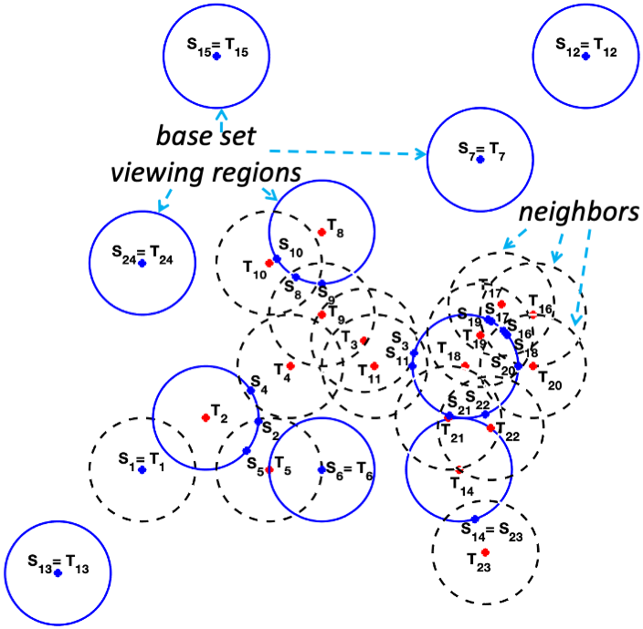
Example: Fig. 7 illustrates the selection of base set circles on a $24$ target example. All isolated sensing circles are first selected as base set circles and removed from $\mathcal{W}$. Next $R(T_{8})$ is randomly selected as a base set circle and removed with its overlapping circles from $\mathcal{W}$. This step repeats for $R(T_{2})$, $R(T_{18})$ and $R(T_{14})$. Finally $R(T_{6})$ is left in $\mathcal{W}$ and selected as the last base set circle.  $\circ$

Initial Sensing node location selection: Each base set circle, $R(T_{i})$ for $i\!\in\!\mathcal{I}$, is used to select initial sensing node locations as follows. If $R(T_{i})$ has no neighbors, no other target’s sensing circles overlap $R(T_{i})$, the target $T_{i}$ at its center is selected as an initial  sensing node location. These are sensing nodes $S_{6},S_{7},S_{12},S_{13},S_{15},S_{24}$ in Fig. 7. Otherwise, $R(T_{i})$ overlaps other sensing circles and sensing nodes are selected on $R(T_{i})$’s perimeter at the midpoint of its overlap with each neighboring circle. These are $S_{4},S_{5}$ on the perimeter of $R(T_{2})$, $S_{9},S_{10}$ on the perimeter of $R(T_{8})$, several sensing nodes on the perimeter of $R(T_{18})$ and $S_{23}$ on the perimeter of $R(T_{14})$ in Fig. 7. The sensing node for each non-isolated base set circle is selected on its perimeter, at the center of its overlaps with the neighboring sensing circles. These are the perimeter of $R(T_{2}),R(T_{8}),R(T_{14}),R(T_{18})$ in Fig. 7. The initial sensing nodes are computed in $O(n)$ time and $n_{s}\!=\!n$ at this stage.

Sensing nodes optimization: Having identified  initial  sensing node locations, the algorithm that solves Problem $\#2$ proceeds much like the solution to Problem $\#1$. Algorithm 1 computes a Hoogeveen path that starts at $S_{1}\!=\!T_{1}$, visits the intermediate sensing nodes in any order and ends at a sensing node that observes the final target $T_{n}$. The Hoogeven path fixes the incidence variables, $\xi_{ij}$, and the sensing nodes are indexed according to the Hoogeven path visitation order as $S_{1},\ldots,S_{n}$. The sum-of-norms cost function

$$Cost(S_{1},\ldots,S_{n})\ =\ \sum_{i=1}^{n}\mbox{$\|S_{i+1}-S_{i}\|$}\vspace{-.08in}$$ (16)

forms a convex function of the sensing node locations. Since each target has its own sensing node at this stage, the viewing variables are set as $\eta_{ij}\!=\!1$ for $j\!=\!i$ and $\eta_{ij}\!=\!0$ for $j\!\neq\!i$ ($i\!=\!1\ldots n$). Each sensing node $S_{j}$ except $S_{1}$ thus may vary in its sensing circle, $R(T_{j})$. Computation of the shortest sensory coverage path under fixed visitation order and fixed viewing assignments forms a convex optimization problem that can be efficiently solved using Algorithm 2 of the previous section.

Figure 8: The $24$ targets example of Fig. 7. The Hoogeveen path through the initial sensing nodes shown as red path, ordered by gray incidence arrows above. The optimized sensory coverage path computed under the Hoogeveen visitation order shown as black path, with the optimized sensing nodes overlaid as blue dots along this path.

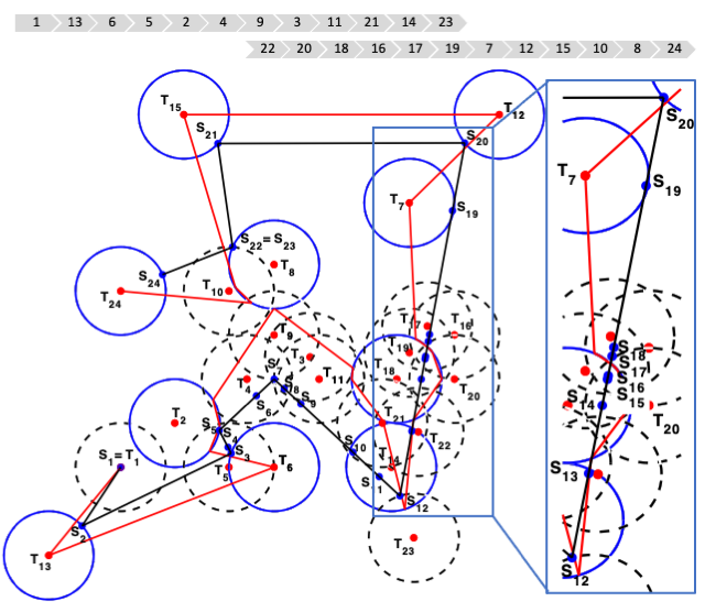
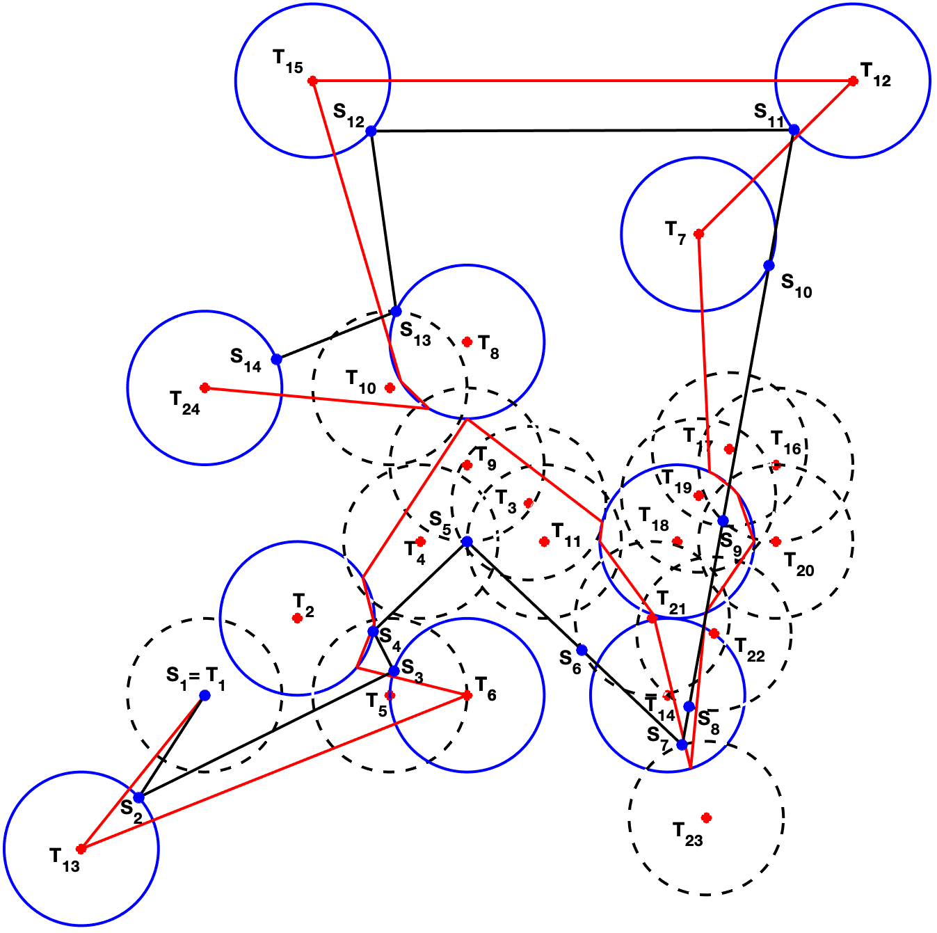
Example: Fig. 8 illustrates the two-stage solution of Algorithm 2 on the $24$ targets example of Fig. 7. The Hoogeveen path passing through the initial sensing nodes was computed in $0.4$ seconds (red path). The sensing node locations are next optimized under the Hoogeveen visitation order as a convex optimization problem, with each sensing node allowed to freely vary in its target-centered sensing circle. The optimized sensory coverage path shown as black path in Fig. 8 was computed in $1.11$ seconds. The $24$ optimized sensing nodes appear as blue dots along the optimized path.  $\circ$

Figure 9: The sensing node reduction in Alg. 3 is illustrated, with intervals identified, sorted, reversed along to place sensing nodes.

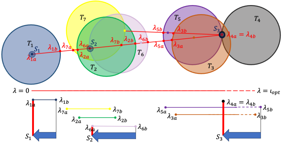
Sensing node reduction: The final stage of the algorithm selects a reduced set of sensing nodes along the optimized sensory coverage path. General sensing node reduction in 2-D environments forms an $NP$-hard set cover problem [38]. However, sensing node reduction along the optimized path can be done in polynomial time as next described.

The overlap segments on the optimized path, denoted as $I_{i}\!=\![a_{i},b_{i}]$ for $i\!=\!1\ldots k$ ($k\!\geq\!n)$, are defined as the intervals along the path where each sensing circle is first entered, at $a_{i}$ and exited, at $b_{i}$. The overlap segments are thus uniquely associated with the sensing circles along the optimized path. Sensing node reduction starts by sorting the overlap segments along the path into list $\mathcal{U}$. Moving in reverse from the end of the optimized path until the first $a_{i}$ entry is found, a sensing node is placed at $a_{i}$, allowing the robot to observe $T_{i}$ and possibly many targets along the $[a_{i},b_{i}]$ segment, since other overlap segments have only begun in the region of $a_{i}$, but none has ended. This is illustrated in Fig. 9, with $S_{3}$ as the first node. All targets viewable from $a_{i}$, $T_{j}$ s.t. $a_{j}\leq a_{i}\leq b_{j}$, are removed from the list of uncovered target intervals $\mathcal{U}$. This process repeats until all targets have been observed, shown in Fig. 9 as $S_{1},S_{2},$ and $S_{3}$.

The sensing node reduction process is summarized as Algorithm  3. Lines 3-6 compute the overlap segments, which are stored in $\mathcal{U}$. Line 7 sorts these segments by their start point, $a_{i}$ for $i\!=\!1\ldots n$. Lines 8-19 select sensing nodes by reversing along $\mathcal{P}$ and removing redundant overlap segments from $\mathcal{U}$, while storing the selected sensing nodes in $S_{min}$. The path $\mathcal{P}$ consists of $n\!-\!1$ line segments checked against $n$ sensing circles to identify overlap segments. Computation and sorting of the overlap segments thus takes $O(n^{2})$ time, then sensing node reduction takes additional $O(n)$ time.

Algorithm 3 Sensing Node Reduction

Input: Targets $\mathcal{T}\!=\!\{T_{1}\ldots T_{n}\}$. Optimized path $\mathcal{P}$. Sensing
  nodes $\mathcal{S}\!=\!\{S_{1}\ldots S_{n}\}$ along $\mathcal{P}$.

1:procedure SensingNodeReduction($\mathcal{T}$, $\mathcal{P}$, $\mathcal{S}$)

2:    $\mathcal{U}\leftarrow\emptyset$,   $\mathcal{S}_{min}\leftarrow\emptyset$

3:    for $i=1$ to $n$ do

4:         $I_{i}\leftarrow OverlapInterval(R(T_{i}),\mathcal{P})$

5:         $\mathcal{U}\leftarrow\mathcal{U}\cup\{I_{i}\}$

6:    end for

7:    Set $\mathcal{U}=SortOverlapSegments(\mathcal{U})$

8:    while $\mathcal{U}\!\neq\!\emptyset$ do

9:         $\mathrm{S}_{new}=\mathcal{U}(end)(a_{i})$

10:         $\mathcal{S}_{min}=\mathcal{S}_{min}\cup\{\mathrm{S}_{new}\}$

11:         Set $j=1$

12:         while $j\leq size(\mathcal{U})$ do

13:             if $\mathrm{S}_{new}\in I_{j}$ then

14:                 Discard $I_{j}$ from $\mathcal{U}$

15:                 $j--$

16:             end if

17:             $j++$

18:         end while

19:    end while

20:    Return (reduced sensing nodes $\mathcal{S}_{min}$ )

21:end procedure

Example: Algorithm 3 was applied to the $24$ sensing nodes located on the optimized sensory coverage path of Fig. 8. The algorithm found the reduced sensing nodes $S_{1},\ldots,S_{14}$ shown in Fig.  10 in $2.0$ seconds. These sensing nodes exploit multi-target views to observe all $24$ targets.  $\circ$

Algorithm 4 Shortest Cover Under Multi-Target Views

Input: Targets $\mathcal{T}\!=\!\{T_{1},\ldots,T_{n}\}$

1:procedure ReducedSensingPath($\mathcal{T}$)

2:     $\mathcal{I}=BaseSetCicrcles(\mathcal{T})$

3:     $\{S_{1},\ldots,S_{n}\}=BaseSetSensingNodes(\mathcal{I},\mathcal{T})$

4:     $\mathcal{P}_{order}$ = Hoogeveen($S_{1},\ldots,S_{n}$)

5:     $\{\xi_{ij}\}\ =\ {\rm Incidence}(P_{order})$

6:     $\eta_{ij}\!=\!1\ {\rm for}\ j\!=\!i,\eta_{ij}\!=\!0\ {\rm for}\ j\!\neq\!i$

7:     ($\mathcal{P},\mathcal{S}_{opt})=\operatorname*{Arg\,Min}{\rm Cost}\big{\{}\{\xi_{ij}\},\{\eta_{ij}\},\mathcal{S},\mathcal{T}\big{\}}$

8:     $\quad{\rm subject\ to}\ S_{1}\!=\!T_{1}\ {\rm and}\ S_{i}\!\in\!R(T_{i})$ $i=2\ldots n$

9:     $\mathcal{S}_{min}$ = SensingNodeReduction($\mathcal{T}$, $\mathcal{P}$, $\mathcal{S}_{opt}$)

10:     $Return\big{(}\mbox{\rm path}\ \mathcal{P},\mbox{\rm reduced sensing nodes}\ \mathcal{S}_{min}\big{)}$

11:end procedure

Figure 10: The $24$ targets example of Fig. 8 showing the optimized sensory coverage path (in black) with reduced sensing nodes $S_{1},\ldots,S_{14}$ that use multi-target views to observe all targets along this path.

The approximation algorithm that solves Problem $\#2$ is summarized as Algorithm  4. Its main steps are base set selection in $O(n)$ time, initial sensing nodes assignment in $O(n)$ time, Hoogeveen path computation in $O(n^{3})$ time, convex optimization in $O(c\cdot n^{2}\ln(1/\epsilon))$ time, and sensing node reduction in $O(n^{2})$ time, $n$ is the number of targets.

Path length bound: Proposition 3 describes the path length approximation bound for Algorithm 4. The proof follows Dumitrescu  [13] with a slightly improved bound.

Proposition 3

When the locations of targets $T_{1},\ldots,T_{n}$ leads to overlapping sensing circles of radius $r$, Algorithm 4 computes in $O(n^{3})$ time a sensory coverage path whose length satisfies the approximation bound

$$l(\mbox{\rm Alg.~{}\ref{alg:overlap_reduce}})\ \leq\ {\color[rgb]{0,0,0}\tfrac{5}{3}}\big{(}9\cdot l_{opt}\!+\!(1\!+\!8\pi)r\big{)}\vspace{-.06in}$$

where $l_{opt}$ is the length of the optimal $S$-to-$T$ sensory coverage path that takes advantage of multi-target views in an obstacle free environment.

Proof: Let $\mbox{$\alpha$}_{opt}$ be the shortest $S$-to-$T$ sensory coverage path that takes advantage of multi-target views, with $l_{opt}$ denoting its length. The optimal path must visit every base set circle, otherwise the targets at the centers of these circles cannot be observed by the robot. Consider the area swept by a disc of radius $2r$ while its center moves along the path $\mbox{$\alpha$}_{opt}$

$$\mathcal{A}=4r\cdot l_{opt}+4\pi r^{2}\vspace{-.06in}$$ (17)

where $4\pi r^{2}$ is the area of two half-discs at the endpoints of $\mbox{$\alpha$}_{opt}$. The area swept by the disc covers all base set circles, each having radius $r$. Since the base set circles are disjoint

$$\mathcal{A}\geq|\mathcal{I}|\cdot(\pi r^{2})\vspace{-.04in}$$

where $|\mathcal{I}|$ is the number of base set circles. Substituting for $\mathcal{A}$ according to Eq. (17) gives

$$|\mathcal{I}|\leq 4(\frac{l_{opt}}{\pi r}+1).\vspace{-.02in}$$ (18)

Next consider the path computed by Alg. 4. It starts at $S_{1}$, visits $S_{2},\ldots,S_{n-1}$ in some order, then ends at $S_{n}$. Using Lemma 1, the length of this path, $l_{H}$, satisfies the bound $l_{H}\leq\tfrac{5}{3}l_{TSP}$ where $l_{TSP}$ is the length of the shortest $S$-to-$T$ path that starts at $S_{1}$ and ends at $S_{n}$. The convex optimization stage of Alg. 4 only shortens the Hoogeveen path. Hence $l(\mbox{\rm Alg.~{}\ref{alg:overlap_reduce}})\leq l_{H}\leq\frac{5}{3}l_{TSP}$.

An alternative path $\mathcal{P}$ that visits the sensing nodes takes advantage of the nodes’ initial locations on the base set circle perimeters and centers. By construction, each base set circle has sensing nodes on its perimeter or a single sensing node at its center. Path $\mathcal{P}$ starts at $S_{1}$ and follows $\mbox{$\alpha$}_{opt}$. Each time $\mbox{$\alpha$}_{opt}$ reaches a base set circle, imagine that the robot’s path executes full circumnavigation of the circle when it contains perimeter sensing nodes, and straight in-and-out motion to its center when the circle contains a sensing node at its center. The path then continues along $\mbox{$\alpha$}_{opt}$ to the next base set circle. The length of this path, $l_{b}$, satisfies the upper bound

$$l_{b}\leq l_{opt}+2\pi r\cdot|\mathcal{I}|+r.\vspace{-.04in}$$

The path that circumnavigates the base-set-circles is longer than the shortest path that visits the sensing nodes. Hence $l_{TSP}\leq l_{b}$ and consequently

$$\begin{array}[]{l}l(\mbox{\rm Alg.~{}\ref{alg:overlap_reduce}})\!\leq\!\tfrac{5}{3}l_{TSP}\!\leq\!\tfrac{5}{3}l_{b}\\[2.0pt] \!\leq\!\tfrac{5}{3}\big{(}l_{opt}\!+\!8\pi r\cdot(\frac{l_{opt}}{\pi r}\!+\!1)+r\big{)}\!=\!\tfrac{5}{3}(9\cdot l_{opt}\!+\!(1\!+\!8\pi)r)\end{array}$$

where we substituted the upper bound (18) for $|\mathcal{I}|$.  $\square$

V Multi-Target Sensory Coverage Among Obstacles with Path Length Bound

This section considers multi-target sensory coverage in the presence of obstacles. We first develop an MINLP problem formulation, then describe an algorithm that approximately solves this problem, followed by sensing node reduction along the sensory coverage path. The section ends with analysis of the algorithm’s path length approximation bound.

Figure 11: (a) The viewing region $V(T_{i})$ of direct lines of sight that start at $T_{i}$ and reach the sensing circle boundary or hit an obstacle before reaching maximal detection range. Occlusion edges are tangent to obstacles or reach sensing circle and obstacle intersection points. (b) The boundary that separates the viewing region $V(T_{i})$ from other obstacle free regions, in green, consists of occlusion edge segments and sensing circle arcs.

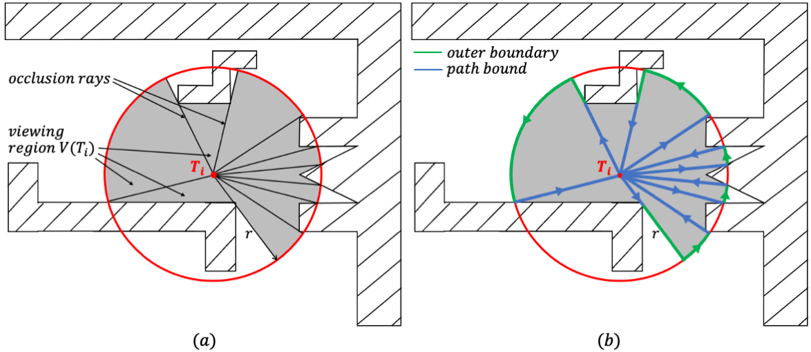
The targets $T_{1},\ldots,T_{n}$ lie in an environment populated by polygonal obstacles that may obstruct sensor views of the targets. The robot can detect targets only along direct lines of sight within detection range $r$. Each target $T_{i}$ can thus be detected from a viewing region, $V(T_{i})$, defined as the set of rays that start at $T_{i}$ and either reach the sensor range limit or hit an obstacle (Fig. 11(a)). Each viewing region consists of triangular radial sectors bounded by occlusion edges. Each occlusion edge is either tangent to an obstacle vertex or edge, or reaches an intersection point of the sensing circle boundary with an obstacle edge (Fig. 11(a)).

In mobile robot sensory coverage, the presence of obstacles implies that targets which can be observed by the robot may not be physically accessible by the robot. This issue is not directly included in our algorithm. Rather, the problem is viewed as optimizing sensing node placements and planning a safe collision-free path between them. We assume that the entire free space can be continually accessed by the robot sensor, and viewing regions are constructed accordingly. If desired, obstacles may be replaced by their configuration space representations.

MINLP formulation: The robot path cost is measured as the sum of the shortest collision free path lengths connecting successive sensing nodes along the robot path

$$Cost(\{S_{1},\ldots,S_{n}\},\{\xi_{ij}\})=\sum_{i=1}^{n}\sum_{j=1,j>i}^{n}\!\xi_{ij}\!\cdot\!l_{min}(S_{j},S_{j+1})\vspace{-.02in}$$

where $l_{min}(S_{j},S_{j+1})\!\geq\!0$ is the length of the shortest collision free path connecting $S_{j}$ and $S_{j+1}$. The incidence variables, $\xi_{ij}$ for $i,j\!\in\!\{1,\ldots,n\}$, are defined as before, $\xi_{ij}=1$ if $T_{j}$ is observed right after $T_{i}$, and 0 otherwise.

The MINLP formulation assumes one sensing node per target, without Big-M constants that allow multi-target views. However, sensing node reduction will be performed along the optimized sensory coverage path among obstacles. Each sensing node, $S_{i}\!\in\mbox{$I\!\!R$}^{2}$, must lie inside the viewing region $V(T_{i})$. This requirement is captured by two constraints

$$||S_{i}-T_{i}||\leq r\hskip 6.00006pt\mathrm{and}\hskip 6.00006ptl_{min}(S_{i},T_{i})=||S_{i}-T_{i}||$$ (19)

where $l_{min}(S_{i},T_{i})$ is the shortest collision free path between $S_{i}$ and $T_{i}$. The inequality $\mbox{\small$||S_{i}\!-\!T_{i}||$}\!\leq\!r$ ensures that $S_{i}$ lies inside $R(T_{i})$, while the equality $l_{min}(S_{i},T_{i})\!=\!\mbox{\small$||S_{i}-T_{i}||$}$ ensures that $S_{i}$ has a direct line of sight to target $T_{i}$.

Problem $\#3$: Given targets $T_{1},\ldots,T_{n}$ in an environment populated by polygonal obstacles, compute the shortest $S$-to-$T$ path, $\mathcal{P}$, that visits sensing nodes $S_{1},\ldots,S_{n}$ such that all targets can be observed from the sensing nodes along direct lines of sight. This problem is formulated as the MINLP optimization problem

$$(\mathcal{S}^{*},\{\xi_{ij}^{*}\})\!=\!\operatorname*{Arg\,Min}_{\mathcal{S},\{\xi_{ij}\},}\ \!\!\bigg{(}\!\sum_{j=i,j>i}^{n}\!\!\xi_{ij}\cdot l_{min}(S_{i},S_{j})\!\bigg{)}$$

where the sensing nodes, $\mathcal{S}\!=\!\{S_{1},\ldots,S_{n}\}$, and incidence variables, $\xi_{ij}$, are subject to the constraints of Eqs (5)-(8) while each sensing node $S_{i}$ must satisfy the viewing constraints of Eq. (19) for $i=1\ldots n$.

Approximation algorithm for multi-target views among obstacles: The algorithm that approximately solves Problem $\#3$ selects initial sensing nodes, finds a sensor node visitation order, optimizes the ordered sensing node locations, then reduces the number of sensing nodes using multi-target views along the optimized path.

The algorithm first selects a base set of disjoint viewing regions from which all targets can be observed along direct lines of sight. The technique is similar to the one used in the previous section. Consider the set of viewing regions, $\mathcal{W}\!=\!\{V(T_{i}):i=1\ldots n\}$. One randomly selects a viewing region from $\mathcal{W}$, then removes this region and its overlaps with other viewing regions from $\mathcal{W}$. This iteration repeats until all viewing regions are removed from $\mathcal{W}$.

Computation of the $n$-target viewing regions requires $O(n\!\cdot\!m^{2}_{r}\log m_{r})$ time, where $m_{r}\leq m$ is the maximum number of obstacle vertices and edges within detection range $r$ of each target, after an $O(n\!\cdot\!m)$ pre-processing step to identify the set of intersecting vertices and edges of cardinality $m_{r}$. Each viewing region boundary consists of at most $m_{r}$ occlusion edges and circular arcs (due to sensor range limits). The existence of an overlap between two viewing regions can be found in $O(m_{r}\log m_{r})$ time using the sweepline algorithm [34]. The entire base set can thus be computed in $O(n^{2}\!\cdot\!m_{r}\log m_{r})$ time. The indices of the base set viewing regions are stored in the set $\mathcal{I}$.

Figure 12: A seven target example showing a base set of viewing regions $V(T_{5}),V(T_{6})$. Initial sensing node locations $S_{1},\ldots,S_{7}$ are selected on the boundaries and centers of the base set viewing regions (see text).

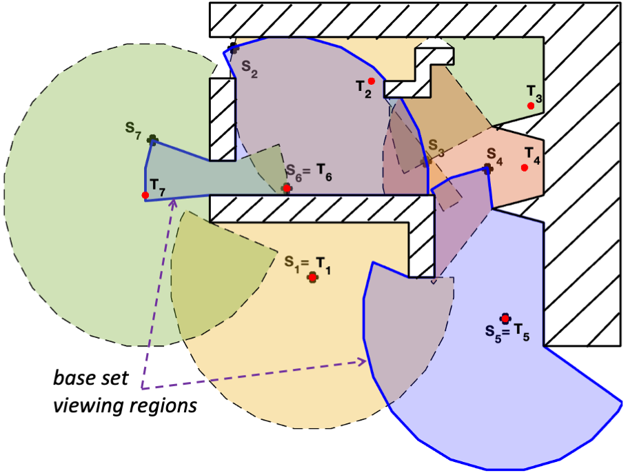
Example: Fig. 12 illustrates the selection of base set viewing regions on a six target example. Initially all viewing regions in $\mathcal{W}$ have overlaps. Viewing region $V(T_{5})$ is randomly selected and removed from $\mathcal{W}$ (including its overlap with region $V(T_{4})$). Viewing region $V(T_{6})$ is selected next, and removed with its overlapping regions $V(T_{2}),V(T_{3}),V(T_{7})$ from $\mathcal{W}$. Hence, the base set is $\mathcal{I}\!=\!\{5,6\}$.  $\circ$

Initial sensing node selection: Each base set viewing region, $V(T_{i})$ for $i\!\in\!\mathcal{I}$, is used to select initial  sensing nodes as follows. If $V(T_{i})$ is an isolated viewing region or intersects an obstacle vertex, the target $T_{i}$ at its center is selected as a sensing node. If $V(T_{i})$ overlaps a neighboring viewing region, $V(T_{j})$, a sensing node $S_{j}$ for the neighboring target $T_{j}$ is selected on the boundary of $V(T_{i})$. These are the sensing nodes $S_{2},S_{3},S_{4},S_{7}$ in Fig. 12. Base regions $V(T_{i})$ with neighbors but without obstacle vertex intersections have $S_{i}$ placed on the boundary of $V(T_{i})$. Sensing nodes selection can be integrated into the overlap computation of the base set viewing regions, thus requiring only $O(n)$ additional time.

Hoogeveen $S$-to-$T$ shortest path approximation: The algorithm that solves Problem $\#3$ proceeds much like the previous problems’ solution. Algorithm 1  is  used  to compute a  Hoogeveen path that starts at $S_{1}\!=\!T_{1}$, visits the sensing nodes $S_{2},\ldots,S_{n-1}$ in some order, and ends at sensing node $S_{n}$ that observes target $T_{n}$. Hoogeveen’s algorithm needs as input a complete graph of shortest collision free paths connecting all sensing nodes in the polygonal environment. The visibility graph [37] contains the shortest collision free paths between all sensing nodes and can be computed in $O((m_{cvx}\!+\!n)^{2}\log(m_{cvx}\!+\!n))$ time [37], where $m_{cvx}\leq m$ is the total number of convex obstacle vertices in the environment, which simplifies the visibility graph. From the constructed visibility graph, the shortest collision free paths between all sensing node pairs can be computed in $O((m_{cvx}\!+\!n)^{3})$ additional time using Johnson’s algorithm [24]. The Hoogeveen path itself then takes $O(n^{3})$ time to compute.

Figure 13: The Hoogeveen $S$-to-$T$ path, shown in red, passes through the sensing nodes $S_{1},\ldots,S_{7}$ shown in Fig. 12. The optimized path is shown in black.

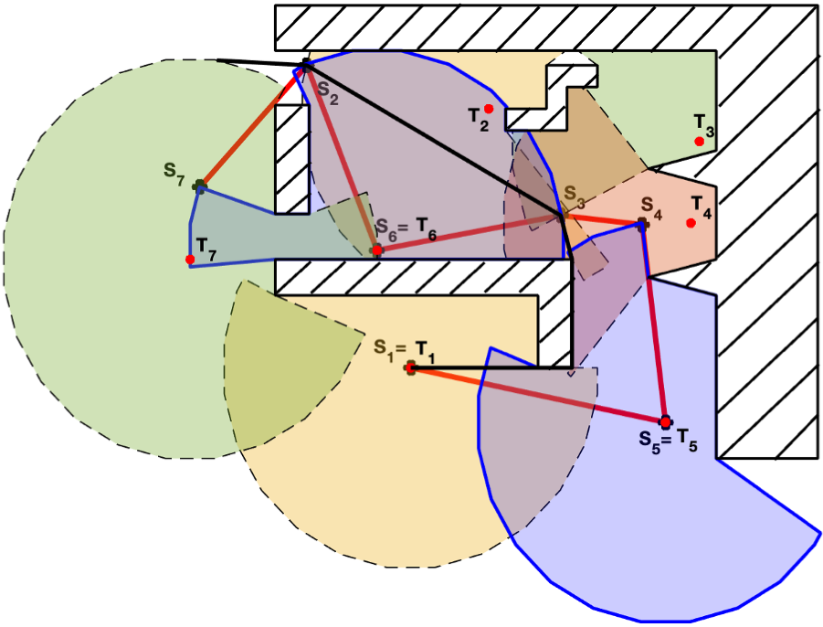
Example: Fig. 13 shows the Hoogeveen path on the seven target example from Fig. 12, computed in .0195 seconds, connecting the initial sensing nodes $S_{1},\ldots,S_{6}$, shown in red.  $\circ$

Sensing node location optimization: The sensing nodes are indexed according to the Hoogeveen path visitation order as $S_{1},\ldots,S_{n}$. The algorithm optimizes the sensing node locations inside obstacle free corridors, defined as follows. The $i^{th}$ corridor is bounded at both ends by linear segments, $w_{i}$ and $w_{i+1}$, that pass through sensing nodes $S_{i}$ and $S_{i+1}$ (bold green segments in Fig.  14). The $i^{th}$ corridor’s left wall is the shortest collision free path connecting the segments’ left endpoints, its right wall is the shortest collision free path connecting the segments’ right endpoints (Fig. 14). Both walls are computed in the path homotopy class of the Hoogeveen path connecting $S_{i}$ and $S_{i+1}$ in the polygonal environment. The $i^{th}$ corridor, called an hourglass [25], contains all shortest collision free paths that connect points of $w_{i}$ with those of $w_{i+1}$ within the path homotopy class, provided that $w_{i}$ and $w_{i+1}$ do not intersect each other (nor their obstacle-free linear extensions).

Figure 14: The seven target example of Fig. 12 showing the connected six corridors bounded by the sensing node $S_{1}\!=\!T_{1}$ (a single-point segment), and then by linear segment of size $\leq 2r$ that lie in the viewing regions $V(T_{H}(i))$ and contain the sensing nodes $S_{H(i)}$ for $i\!=\!2\ldots 7$ (bold green segments marked with $w_{i}$). The optimized coverage path shown in black, with full set of sensing nodes marked. After sensing node reduction, the first reduced sensing node, the red star, observes $T_{1}$ and $T_{5}$, the second star at $S_{3}$ observes $T_{2},T_{3},T_{4},T_{6}$, and the final reduced sensing node, coincident with $S_{7}$ observes $T_{7}$

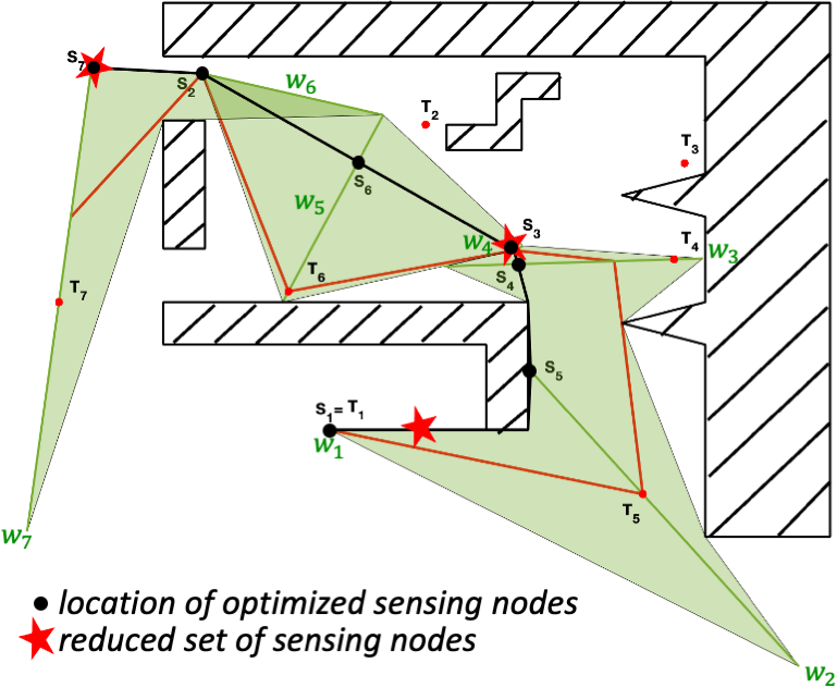
The corridors are constructed as follows. The first corridor is spanned by the sensing node $S_{1}\!=\!T_{1}$ (a single-point segment) and the linear segment of size $\leq 2r$ that lies in the viewing region $V(T_{2})$ and contains sensing node $S_{2}$ ($w_{2}$ in Fig. 14). Each subsequent corridor is bounded by linear segments $w_{i}$ and $w_{i+1}$ of size $\leq 2r$ that lie in their viewing regions $V(T_{i})$ and $V(T_{i+1})$ and contain the sensing nodes $S_{i}$ and $S_{i+1}$ (Fig. 14). The segments $w_{i}$ and $w_{i+1}$ are clipped into collision free sub-segments when they overlap nearby obstacles. Computation of the $n\!-\!1$ corridors takes $O(nm^{2}\log m\!+\!m\!\cdot\!n)$ time.

The corridors are next partitioned into triangular cells whose vertices lie on the corridor walls (Fig. 14). The triangulation is linear in the sense that the Hoogeveen path successively crosses each of these triangles, thus imposing linear order on the triangles of each corridor. Using boundary constrained triangulation  [33], triangulation of the $n\!-\!1$ corridors takes $O(n\!\cdot\!m\log(m))$ time.

Example: Fig. 14 shows the corridors that surround the Hoogeveen path for the seven target example of Fig.  12, computed and triangulated in 1.77 seconds.   $\circ$

The sensing nodes locations are next optimized within the corridors as follows. Let the $i^{th}$ corridor consist of $k_{i}$ triangles. Let $e_{i,0},\ldots,e_{i,k_{i}}$ denote the triangle edges crossed by the Hoogeveen path, indexed according to the linear order imposed by the Hoogeveen path crossing the edges. The triangle edges $e_{i,0}\!=\!w_{i}$ and $e_{i,k_{i}}\!=\!w_{i+1}$ bound the $i^{th}$ corridor and contain the sensing nodes $S_{i}$ and $S_{i+1}$. To ensure that each sensing node observes its target, each $S_{i}$ varies in a segment formed by the intersection of $e_{i,0}$ with the viewing region $V(T_{i})$, such that the segment contains the initial sensing node $S_{i}$.

The path cost is now measured as a function of the path via points that vary on the triangle edges crossed by the Hoogeveen path. These via points are denoted $\{p_{i,0},\ldots,p_{i,k_{i}}\}$ for $i\!=\!1\ldots n\!-\!1$, and the path cost is

$$Cost(\{p_{1,j}\}_{i=1..n-1,j=0..k_{i}})\\ \!=\!\sum_{i=1}^{n-1}\sum_{j=0}^{k_{i}-1}\mbox{$\|p_{i,j+1}\!-\!p_{i,j}\|$}\vspace{-.01in}$$

such that $p_{1,0}\!=\!\mbox{\small$T$}_{1}$ and $p_{i+1,0}\!=\!p_{i,k_{i}}$ for $i\!=\!1\ldots n\!-\!2$. Each corridor entry point, $p_{i,0}$, is subject to the viewing constraint

$$p_{i,0}\in e_{i,0}\cap V(T_{i})\hskip 10.00002pt\mbox{\hskip 5.0pt $i=1\ldots n\!-\!1$}$$

such that the $i^{th}$ viewing sub-segment contains the initial sensing node $S_{i}$ while the remaining via points are subject to the triangle edge constraints

$$p_{i,j}\in e_{i,j}\hskip 10.00002pt\mbox{\hskip 15.00002pt $i=1\ldots n-1,\,j=1\ldots k_{i}$.}\vspace{-.06in}$$

The path cost forms a convex function of the via points when they vary on linear segments. Moreover, the straight line segments between neighboring via points lie in obstacle free triangular cells. Convex optimization can thus efficiently optimize the sensing node locations within the corridors that surround the Hoogeveen path, as illustrated in the following example.

Example: Consider again the seven target example. Fig.  14 shows the sensory coverage path (in black) obtained by optimizing the path via point locations, starting from the initial sensing nodes located on the Hoogeveen path (shown in red). The optimized path was computed in .589 seconds, with sensing nodes located at $S_{1}\!=\!T_{1}$, then at $S_{i}\!=\!p_{i,0}$ for $i\!=\!2\ldots n-1$ and finally at $S_{n}\!=\!p_{n-1,k_{n-1}}$ where $n=7$.  $\circ$

Sensing node reduction: Sensing node reduction is performed by Algorithm 3. The algorithm now requires the overlaps of the optimized path with the $n$ viewing regions. These overlaps can be computed in $O(n^{2}\!\cdot\!m_{r})$ time, then fed into Algorithm 3 which selects in $O(n)$ additional time a reduced set of sensing nodes. These nodes observe all targets using multi-target line of sight views. Fig. 14 shows the reduced sensing nodes along the optimized path, computed in .0279 seconds.

Algorithm 5 Multi-Target Cover Among Obstacles

Input: Targets $\mathcal{T}\!=\!\{T_{1},\ldots,T_{n}\}$, polygonal obstacle ver-
            tices $\mathcal{O}$, $|\mathcal{O}|=m$.

1:procedure ReducedSensingPath($\mathcal{T}$, $\mathcal{O}$)

2:    ​ $\{V(T_{1}),\ldots,\!V(T_{n})\}=ViewingRegions(\mathcal{T},\mathcal{O})$

3:    ​ $\mathcal{I}=BaseSetCicrcles(\mathcal{T},\mbox{\small$\{V(T_{i})\}$})$

4:    ​ $\{S_{1},\ldots,S_{n}\}=BaseSetSensingNodes(\mathcal{I},\mbox{\small$\{V(T_{i})\}$})$

5:    $\mathcal{V}=VisibilityGraphShortestPaths(\{S_{1},\ldots,S_{n}\},\mathcal{O})$

6:    ​ $\mathcal{P}_{order}$ = Hoogeveen($S_{1},\ldots,S_{n},\mathcal{V}$)

7:    ​ $\{\xi_{ij}\}\ =\ {\rm Incidence}(P_{order})$

8:     ($\mathcal{P},\mathcal{S}_{opt})=\operatorname*{Arg\,Min}{\rm Cost}\big{\{}\{\xi_{ij}\},\mathcal{S},\mathcal{T}\big{\}}$

9:     $\quad{\rm subject\ to}\ S_{1}\!=\!T_{1}\ {\rm and}\ S_{i}\!\in\!e_{i,0}\cap\mbox{\small$V(T_{i})$}$ $i=1\ldots n$

10:     $\mathcal{S}_{min}$ = SensingNodeReduction($\mathcal{T}$, $\mathcal{P}$, $\mathcal{S}_{opt}$)

11:     $Return\big{(}\mbox{\rm path}\ \mathcal{P},\mbox{\rm reduced sensing nodes}\ \mathcal{S}_{min}\big{)}$

12:end procedure

The approximation algorithm that solves Problem $\#3$ is summarized as Algorithm 5. It consists of seven stages. The $n$ viewing regions are computed in $O(n\!\cdot\!m^{2}_{r}\log m_{r})$ time, where $m_{r}$ is the maximum number of obstacle vertices and edges within detection range $r$ of each target. Next, a base set of viewing regions and initial sensing nodes are selected in $O(n^{2}m_{r}\log m_{r})$ time. Shortest obstacle free paths between sensing nodes are computed in $O((n+m_{cvx})^{3})$ time. The Hoogeveen path that passes through the sensing nodes is computed in $O(n^{3})$ time. Obstacle free corridors are next computed and triangulated in $O(m^{2}_{r}\log m_{r}\!+\!m\!\cdot\!n)$ time. Convex optimization of the path via points is performed in $O(kn^{2}\ln(1/\epsilon))$ time. Finally, sensing node reduction is performed in $O(n^{2}\cdot m_{r})$ time.

Path length approximation bound: The following proposition assumes that all base set viewing regions have some area $A_{i}>0$ which is captured by a radius $\rho_{i}$ such that $A_{i}=\pi\rho_{i}^{2}$ for $i\!=\!1\ldots n$.

Proposition 4

Let targets $T_{1},\ldots,T_{n}$ be located among polygonal obstacles. Let a point robot move in the freespace using a line-of-sight coverage sensor of detection range $r$. Algorithm 5 computes in $O((m\!+\!n)^{3}\log(m\!+\!n))$ time a sensory coverage path whose length satisfies the approximation bound

$$l(\mbox{\rm Alg.~{}\ref{alg:overlap_obstacles}})\leq\tfrac{5}{3}\big{(}(1\!+\!8\frac{r^{2}}{\bar{\rho}^{2}})\cdot l_{opt}+2r\!\cdot\!m\big{)}+c\vspace{-.05in}$$

where $l_{opt}$ is the length of the optimal $S$-to-$T$ coverage path in the polygonal environment, $m$ is the total number of obstacle vertices, $\bar{\rho}\!\leq\!r$ is the radius of a circle with area equal to the average base set viewing region areas and $c\!=\!(\tfrac{5}{3}\!\cdot\!\tfrac{8r^{2}}{\bar{\rho}^{2}}\!\cdot\!\pi+2)r$ is a constant.

Proof: Let $\mbox{$\alpha$}_{opt}$ be the shortest $S$-to-$T$ sensory coverage path, with length $l_{opt}$. The optimal path must visit every base set viewing region, $V(T_{i})$ for $i\!\in\!\mathcal{I}$, otherwise the target $T_{i}$ at the center of $V(T_{i})$ cannot be observed by the robot. Consider the area swept by a disc of radius $2r$ while its center moves along $\mbox{$\alpha$}_{opt}$

$$\mathcal{A}=4r\cdot l_{opt}+4\pi r^{2}\vspace{-.06in}$$ (20)

where $4\pi r^{2}$ is the area of two half-discs at the endpoints of $\mbox{$\alpha$}_{opt}$. Since each $V(T_{i})$ lies in a sensing circle of radius $r$ centred at $T_{i}$, the area swept by the disc of radius $2r$ along $\mbox{$\alpha$}_{opt}$ covers all base set viewing regions. By construction, the base set viewing regions are disjoint and contain areas equal to circles with radius $\rho_{i}$ for $i\!\in\!\mathcal{I}$. Hence

$$\mathcal{A}\geq\pi\cdot\sum_{i=1}^{|\mathcal{I}|}\rho^{2}_{i}\vspace{-.06in}$$ (21)

where $|\mathcal{I}|$ is the number of base set viewing regions. Using the identity

$$\sum_{i=1}^{|\mathcal{I}|}\rho^{2}_{i}\geq\frac{1}{|\mathcal{I}|}\cdot\big{(}\sum_{i=1}^{|\mathcal{I}|}\rho_{i}\big{)}^{2}$$

we obtain the lower bound on $\mathcal{A}$

$$\mathcal{A}\geq|\mathcal{I}|\cdot\pi\bar{\rho}^{2}$$

where $\bar{\rho}\!=\!\sum_{i=1}^{|\mathcal{I}|}\rho_{i}/|\mathcal{I}|$ is the average radius of the base set viewing region areas. Substituting for $\mathcal{A}$ according to Eq.  (20) gives

$$|\mathcal{I}|\leq\frac{4r}{\pi\bar{\rho}^{2}}(l_{opt}+\pi r).$$ (22)

The $S$-to-$T$ Hoogeveen path computed by Algorithm 5 starts at $S_{1}\!=\!T_{1}$, visits $S_{2},\ldots,S_{n-1}$ in any order, then ends at $S_{n}$ within detection range of $T_{n}$. Using Lemma 1, the length of this path, $l_{H}$, satisfies the bound $l_{H}\leq\tfrac{5}{3}l_{TSP}$ where $l_{TSP}$ is the length of the shortest $S$-to-$T$ path. The convex optimization step of Alg. 5 only shortens the Hoogeveen path. Hence $l(\mbox{\rm Alg.~{}5)}\leq l_{H}\leq\frac{5}{3}l_{TSP}$.

An alternative path, $\mathcal{P}$, takes advantage of the sensing node locations on the base set viewing regions’ perimeters and centers. Path $\mathcal{P}$ starts at $S_{1}$ and moves along $\mbox{$\alpha$}_{opt}$. When $\mbox{$\alpha$}_{opt}$ reaches a base set viewing region, $\mathcal{P}$ circumnavigates the viewing region’s outer perimeter when the perimeter contains sensing nodes, or executes a straight in-and-out motion to its center when a single sensing node lies at its center. The path then continues along $\mbox{$\alpha$}_{opt}$ to the next base set viewing region.

The length of $\mathcal{P}$, $l_{b}$, satisfies the following upper bound. Because the base set viewing regions are disjoint, each obstacle vertex lies in a single base set viewing region and bounds at most one occlusion edge. A full tour of a base set viewing region perimeter traverses each occlusion edge and each sensing circle arc once. If $m_{r}$ denotes the total number of obstacle vertices within detection range of the targets, the length of $\mathcal{P}$ is bounded by

$$l_{b}\leq l_{opt}+2r\cdot(\pi\!\cdot\!\mbox{\small$|\mathcal{I}|$}+m_{r}+1)$$

where the term $2\pi r\mbox{\small$|\mathcal{I}|$}$ bounds the total length of the circular arcs and obstacle edges on the viewing regions’ perimeters, while the term $2rm_{r}$ bounds the total length of the viewing regions occlusion edges. When a single sensing node lies at the center of a base set viewing region, the detour of length $2r$ to this node is upper bounded by $2\pi r$.

The alternative path $\mathcal{P}$ starts at $S_{1}$, circumnavigates the base set viewing regions while visiting the sensing nodes $S_{2},\ldots,S_{n-1}$, then ends at $S_{n}$. This path is longer than the optimally shortest path that starts at $S_{1}$, visits the same intermediate nodes, then ends at $S_{n}$. Thus $l_{b}\geq l_{TSP}$ and the path length bound on Algorithm 5 becomes

$$l(\mbox{\rm Alg.~{}\ref{alg:overlap_obstacles}})\leq\tfrac{5}{3}l_{TSP}\!\leq\!\tfrac{5}{3}l_{b}\leq\tfrac{5}{3}\big{(}l_{opt}\!+\!2r\cdot(\pi\!\cdot\!|\mathcal{I}|+m+1)\big{)}\,$$ (23)

Substituting the upper bound for $|\mathcal{I}|$ specified in Eq. (22) and $m_{r}\leq m$ gives the path length bound

$$l(\mbox{\rm Alg.~{}\ref{alg:overlap_obstacles}})\leq\tfrac{5}{3}\big{(}(1\!+\!8\frac{r^{2}}{\bar{\rho}^{2}})\cdot l_{opt}+2r\!\cdot\!m\big{)}+c$$

where $c\!=\!(\tfrac{5}{3}\!\cdot\!\tfrac{8r^{2}}{\bar{\rho}^{2}}\!\cdot\!\pi+2)r$ is a constant.  $\square$

Remark: One can construct several variations on the path length bound of Algorithm 5. One example follows. Given an environment and targets, $|\mathcal{I}|$ is a known quantity. Additionally, the viewing region areas can easily be computed with the knowledge $\mathcal{A}\geq\sum_{i=1}^{|\mathcal{I}|}area(V(T_{i}))$. Hence, one can replace $\mathcal{A}$ with the average, $\mathcal{A}\geq|\mathcal{I}|\cdot E[area(V_{i\in\mathcal{I}})]$. This can serve as the starting point for developing probabilistic path length bounds. By using sample data points or known distributions, the expected value for the base set area or number of obstacle vertices could be substituted into Eq. (23) to generate a predicted bound

$$l_{b}\leq l_{opt}+2\cdot r\big{(}\pi\cdot\frac{4rl_{opt}+4\pi r^{2}}{E[area(V_{i\in\mathcal{I}})]}+m\big{)}$$

$$l_{b}\leq(1+\frac{8\pi\cdot r^{2}}{E[area(V_{i\in\mathcal{I}})]})\cdot l_{opt}+2\cdot r\cdot m+\tilde{c}$$

where $\tilde{c}$ is a constant. $\circ$

VI Conclusion

This paper considered three successively more demanding mobile robot sensory coverage problems: multi-target coverage in obstacle free environments with non-overlapping sensing circles centered at the targets, multi-target coverage in obstacle free environments with possibly overlapping sensing circles that allow multi-target views, and multi-target coverage in environments populated by obstacles that may obstruct sensor views of the targets. All three problems were formulated as NP-Hard MINLP optimization problems.

For each problem, we introduced novel approximation algorithms that can be computed in polynomial time. All three problems were solved in roughly two stages. Initial sensing node locations were selected and a visitation order for these nodes was computed in polynomial time. Then efficient convex optimization was used to optimize the sensing node locations, yielding the shortest sensory coverage path under the set visitation order. In the second and third problems, multi-target views were used to reduce the number of sensing nodes, when possible. The algorithm solving the third problem uses obstacle obstructed viewing regions and shortest collision free path between sensing nodes to enable highly competitive execution times.

The paper developed path length bounds for the three algorithms, expressed in terms of each problem’s optimal path length. These path length bounds provide limits for the gap between the exact solutions for these NP-hard problems and our polynomial time approximate solutions. Finally, all algorithms have been fully implemented in MATLAB with software available as part of the paper.

Future research will focus on two areas. First, there is a need to efficiently search for and inspect multiple targets whose position is only approximately known to the robot. The robot must efficiently inspect viewing neighborhoods surrounding these targets, with provable efficiency bounds. Next, while the general environment layout might be known to the robot, a priori unknown obstacles may be encountered during the robot’s actions. Here, too, there is a need forprovable efficiency bounds, most likely expressed in terms of learned probabilistic obstacle distributions and percentile sensory coverage bounds that use these distributions. The techniques and algorithms described in this paper provide a strong foundation for future work on these problems.

Our future research also aims to extend the MINLP framework to 3-D robot sensory coverage and inspection problems. Robotic agents can efficiently inspect exteriors of 3-D structures that form natural extensions of the planar environments considered in this paper. When a structure’s exterior is only approximately known to the robot, sensory coverage and inspection becomes a volumetric 3-D planning problem. Our MINLP optimization framework can model sensors with convex 3-D footprints. Hence, the techniques described in this paper have a good chance of providing highly efficient algorithms even for the most challenging 3-D sensory coverage and inspection planning problems.

Appendix A Proof of Proposition 2

. To analyze the approximation bound, we must find the worst case ratio $(l_{TSP}/l_{alg})$ over all possible arrangements of targets, where $l_{TS}$ is the TSP path ($\mathcal{P}_{TSP}$) through all targets, and $l_{alg}$ is the shortest possible sensing path ($\mathcal{P}_{CPP}$) that views all targets . We begin by assuming that the worst case arrangement of $n$ targets consists of sensing circles arranged in a closely packed linear fashion (see Figure 5). This assumption will be analyzed below.

The shortest TSP path between the targets in this arrangement is easily characterized. To characterize the shortest sensing path and its associated sensing locations, we use the Karush-Kuhn-Tucker (KKT) optimality conditions. We first analyze the case of an odd number of targets. Let $T_{1}$ and $T_{n}$ be the start node and final target, respectively (see Fig. 15 for a seven target example). The optimal sensing path must contain a sensing node at $T_{1}$ and $n-1$ sensing nodes lying in the remaining target sensing regions. One can show that in a linear packing of sensor regions, the shortest path is defined by four sensing node locations: $S_{1}$ (located at $T_{1}$), $S_{2}$ in the sensing region around $T_{2}$, $S_{n-1}$ in the sensing region around $T_{n-1}$, and $S_{n}$ on the boundary of the sensing region surrounding $T_{n}$. The length of such a path, $||P||$, takes the form (see Fig. 15):

$$||P|| = ||P_{1}||+||P_{2}||+||P_{3}||$$

$$= ||S_{2}-T_{1}||+||S_{n-1}-S_{2}||+||S_{n}-S_{n-1}||.$$

We seek to minimize $||P||$, subject to the constraint that the key sensing nodes lie in their associated sensing regions:

$$||S_{2}-T_{2}||\leq R;\ \ \ \ ||S_{n-1}-T_{n-1}||\leq R;\ \ \ \ ||S_{n}-T_{n}||\leq R.$$

Define the Path Lagrangian, $\mathcal{L}_{P}$ as:

$$\mathcal{L}_{P} = ||P||+\lambda_{1}(||S_{2}-T_{2}||-R)$$

$$+ \lambda_{2}(||S_{n-1}-T_{n-1}||-R)+\lambda_{3}(||S_{n}-T_{n}||-R).$$

The minimal path length necessary KKT conditions are:

$$\frac{\partial\mathcal{L}}{\partial S_{2}} = \frac{S_{1}-T_{2}}{||S_{2}-T_{2}||}-\frac{S_{n-1}-S_{2}}{||S_{n-1}-S_{2}||}+\lambda_{1}\frac{S_{2}-T_{2}}{||S_{2}-T_{2}||}$$

$$\frac{\partial\mathcal{L}}{\partial S_{n-1}} = \frac{S_{n-1}-S_{2}}{||S_{n-1}-S_{2}||}-\frac{S_{n}-S_{n-1}}{||S_{n}-S_{n-1}||}$$

$$\quad+\lambda_{2}\frac{S_{n-1}-T_{n-1}}{||S_{n-1}-T_{n-1}||}$$

$$\frac{\partial\mathcal{L}}{\partial S_{n}} = \frac{S_{n}-S_{n-1}}{||S_{n}-S_{n-1}||}+\lambda_{3}\frac{S_{n}-T_{n}}{||S_{n}-T_{n}||}$$

Since the ratios in these expressions can be interpreted as unit vectors, the KKT conditions yield insight into the shortest sensing path geometry. Figure 15 shows the geometry of the KKT conditions for an odd number of targets in the worst case target geometry.

Figure 15: Geometry of KKT conditions for odd number of targets.

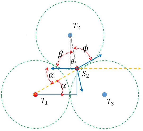
The first condition in Eq. (A) (see Fig. 16) dictates that sensing node $S_{2}$ must be positioned so that the line underlying $\vec{S_{2}T_{2}}$ bisects the angle between the lines underlying $\vec{T_{1}S_{2}}$ and $\vec{S_{2}S_{n-1}}$. From Figure 16, one can calculate that at a minimal path length, the angle between $\vec{T_{2}S_{2}}$ and a vertical line, denoted $\theta^{*}_{o}$, is the solution to the following equation

$$\frac{(\sqrt{3}-\cos(\theta^{*}_{odd}))}{(1+\sin(\theta^{*}_{odd}))}=\tan(2\theta^{*}_{odd})$$ (25)

Using this result, the shortest path length for an odd number of sensing regions is

$$||P_{odd}||\ =\ R[n-4+\kappa_{odd}(\theta^{*}_{odd})]$$ (26)

where

$$\kappa_{o}(\theta^{*}_{o})=2\big{[}(1+\sin\theta^{*}_{o})^{2}+(\sqrt{3}-\cos\theta^{*}_{o})^{2}\big{]}^{1/2}-2\sin\theta^{*}_{o}$$ (27)

Figure 16: Detailed Geometry of KKT condition around sensing node $S_{2}$

The shortest path length for an even number of targets can be analyzed in a similar way. The shortest path length in this case is

$$\begin{split}R\big{[}(\frac{n-3}{2}-\sin\theta^{*}_{even})^{2}+(\cos\theta^{*}_{even}-\frac{\sqrt{3}}{2})^{2}\big{]}^{1/2}-R\end{split}$$

where $\theta^{*}_{even}$ is the solution to the following equation:

$$\frac{\sqrt{3}-\cos\theta^{*}_{even}}{1+\sin\theta^{*}_{even}}=\frac{\tan\theta^{*}_{even}-\eta}{1+\eta\tan(2\theta^{*}_{even})}$$

and $\eta=(2\cos\theta^{*}_{even}-\sqrt{3})/(n-3-2\sin\theta^{*}_{even})$.

One can show that as $n$ increases, $\theta^{*}_{even}\rightarrow\theta^{*}_{odd}$, and that $||P_{even}||$ is very well approximated by the expression of $||P_{odd}||$. In fact, $||P_{odd}||$ in Eq. (26) is an under approximation of the path length, which ensures that Eq. (13) is the worst case bound. Thus, $\kappa^{\prime}_{o}=\kappa_{o}(\theta^{*}_{o})$ yields the shortest optimal path, and the tightest bound in Eq. (26).

Worst Case Target Arrangement. We next analyze the claim that the packed linear arrangement of target sensing regions in Figure 15 leads to the worst case ratio of the target TSP path length, $l_{TSP}$, to the shortest sensing path length, $l_{CPP}$. Our goal is the find the target locations that maximize the ratio

$$\Delta\ \triangleq\ \frac{l_{TSP}^{*}}{l^{*}_{CPP}}.$$

The general proof proceeds by induction. Here we sketch the first few steps of the induction process.

As above, we first develop conditions for extremal values of the ratio $\Delta$. The goal is to maximize $\Delta$ with respect to the choice of target locations (which is the same as minimizing $-\Delta$), subject to the $(n-1)(n-2)/2$ overlap constraints that no two sensing regions overlap, and that target node $T_{1}$ is fixed to a specific location:

$$\min_{T_{2},\ldots,T_{n}} - \Delta(T_{2},\ldots,T_{n})$$ (28)

$${\rm subject\ to:} \ ||T_{j}-T_{i}||^{2}\geq 4r^{2}$$

for $i=1,\ldots,(n-1)$ and $j=2,\ldots,n$.

If the $\Delta$ Lagrangian is defined by:

$$\mathcal{L}_{\Delta}(\mathcal{N},\vec{\lambda})\ =\ -\Delta+\sum_{i=1}^{n-1}\ \sum_{j=i+1}^{n}\ \lambda_{i,j}\big{(}r^{2}-||T_{j}-T_{i}||^{2}\big{)}$$

then the Karush-Kuhn-Tucker (KKT) conditions for a constrained minimum are:

$$0 \in -\frac{\partial\mathcal{L}_{\Delta}(T_{2},\ldots,T_{n},\vec{\lambda})}{\partial T_{k}}=-\frac{\partial\Delta}{\partial T_{k}}$$

$$\ \ \ \ +2\sum_{j=k+1}^{n}\lambda_{j,k}(T_{j}-T_{k})-2\sum_{i=k-1}^{n}\lambda_{k,j}(T_{l}-T_{i})$$

$$0 \geq 4r^{2}-||T_{j}-T_{i}||^{2}$$ (30)

$$0 \leq \lambda_{i,j}$$ (31)

$$0 = \lambda_{i,j}(4r^{2}-||T_{j}-T_{i}||^{2})$$ (32)

where $i=2,\ldots,(n-1)$ in (A)-(32) and $j=(i+1),\ldots,n$ (with $i\neq j$) in Eq.s (30)-(32). To calculate $\partial\Delta/\partial T_{j}$, for $j=2,3$,

$$\frac{\partial\Delta}{\partial T_{j,i}}=\lim_{\vec{\mu_{i}}\rightarrow 0}\bigg{[}\frac{\Delta(T_{j,i}+\mu_{i})-\Delta(T_{j,i})}{\mu_{i}}\bigg{]}$$

where $i=x$ or $i=y$, and $\vec{\mu}=\begin{bmatrix}\mu_{x}&\mu_{y}\end{bmatrix}$ denotes small perturbations of a target’s Cartesian locations.

Since function $\Delta$ may not be convex, conditions (A) - (32) are only necessary conditions for a maximal value of $\Delta$. Note that the geometry of $\mathcal{P}_{CPP}$ and/or $\mathcal{P}_{TSP}$ may change abruptly with small changes in target placements. In these cases, function $\Delta$ can be non-smooth, and $\partial\Delta/\partial T_{i}$ must be interpreted as a generalized (set-valued) gradient.

A-A Case of Two Targets

Let two targets, $T_{1}$ and $T_{2}$, be separated by a distance $2r+\mu$, where $\mu\geq 0$. One can see by inspection that $l_{TSP}^{*}=2r+\mu$ and $l^{*}_{CPP}=r+\mu$. Thus,

$$\Delta=\frac{l_{TSP}^{*}}{l^{*}_{CPP}}=\frac{2r+\mu}{r+\mu}.$$

This ratio takes its largest value when $\mu\rightarrow 0$. I.e., when the boundaries of the circular sensing regions $R(T_{1})$ and $R(T_{2})$ nearly touch. Equivalently, the non-overlapping constraint is active at the maximum.

A-B Case of Three Targets

For targets $T_{1}$, $T_{2}$, and $T_{3}$, let $T_{1}$ be fixed to a given location. Since $\Delta$ may not be convex, its extrema may occur when no, some, or all constraints are active. We first show that $\Delta$ cannot be maximized under with no active constraints. We then analyze the cases of one, two, and three active constraints, concluding that $\Delta$ is maximized when the three targets form the smallest possible equilateral triangle.

KKT condition (32) implies that if each pair of targets is more than $2r$ apart, then $\lambda_{1,2}=\lambda_{1,3}=\lambda_{2,3}=0$, and an extremum in $\Delta$ occurs when the following two conditions hold simultaneously:

$$\vec{0}\ \in\ -\frac{\partial\Delta}{\partial T_{2}};\ \ \ \ \vec{0}\ \in\ -\frac{\partial\Delta}{\partial T_{3}}\ .$$ (33)

If any derivative in (33) is non-zero for all unconstrained target locations, the unconstrained KKT conditions are not satisfied. Without loss of generality, initially assign a reference frame with origin at $T_{1}$ and whose $x$-axis is collinear with $\overrightarrow{T_{1}T_{2}}$. In this reference frame, the problem is symmetrical with respect to the $x$-axis. Hence, we only analyze the case where $T_{3,y}$, the $y$-coordinate of target $T_{3}$, is positive. The symmetric case, where $T_{3,y}<0$, is identical.

Figure 17: Variations in the geometry of $\mathcal{P}_{CPP}$ with respect to target location when no constraints are active. Target $T_{3}$ cannot lie in circular yellow regions, where constraints must be active. When $T_{3}$lies in Region I, $\mathcal{P}_{CPP}$ is a straight line from $T_{1}$ to the boundary of $R(T_{3}^{I})$. When $T_{3}$ lies in Region II, $\mathcal{P}_{CPP}$ is a two segment path intersecting the boundaries of $R(T_{2})$ and $R(N^{II}_{3})$. When $T_{3}$ lies in Region III, the targets must be relabeled, with the relabeled problem falling into Region I or Region II.

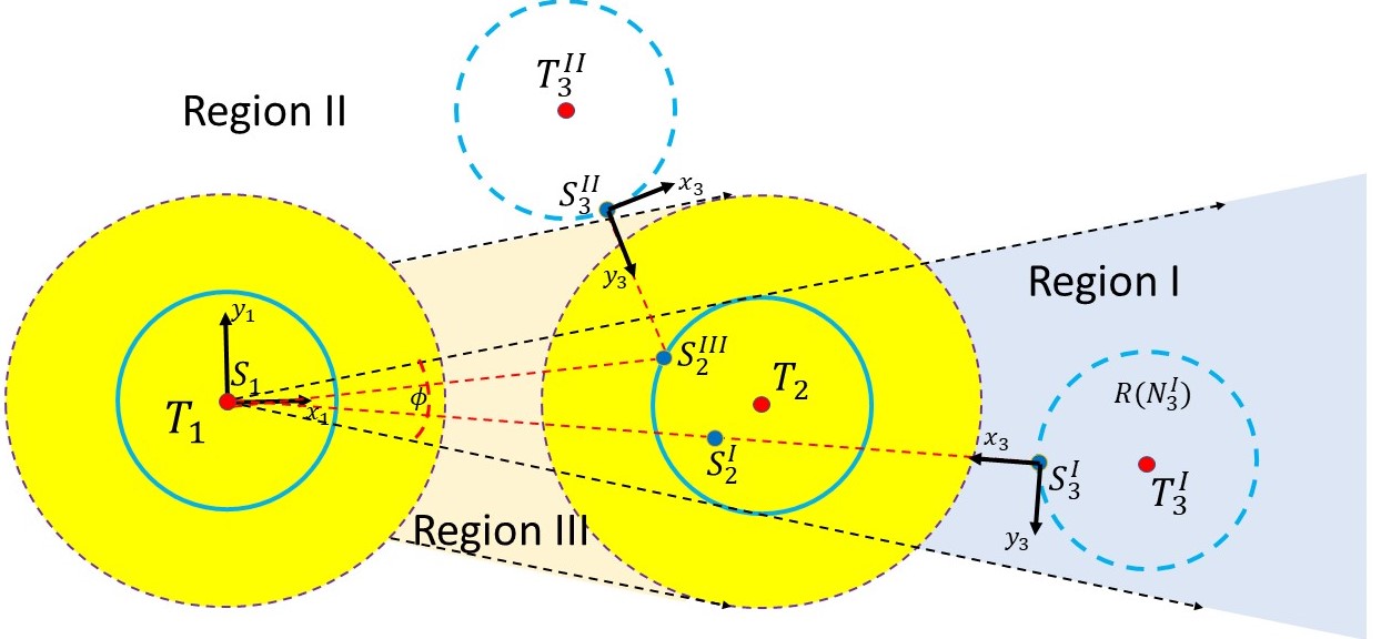
Figure 17 shows how path $\mathcal{P}_{CPP}$ changes with respect to placements of $T_{3}$. When $T_{3}$ lies in Region I, $\mathcal{P}_{CPP}$ is a straight line passing through $R(T_{2})$, and it orthogonally intersects the boundary of $R(T_{3})$. Sensing node $S_{2}$ can placed anywhere along the intersection of $\mathcal{P}_{CPP}$ and $R(T_{2})$.

When $T_{3}$ lies in Region II, $\mathcal{P}_{CPP}$ is a two segment path. The first segment intersects the boundary of $R(T_{2})$ at sensing location, $S_{2}$, whose location is a solution to the following two equations, which are derived from shortest path conditions:

$$\frac{(T_{2}-S_{2})\cdot(T_{3}-S_{2})}{r||T_{3}-S_{2}||} = \frac{(T_{1}-S_{2})\cdot(T_{3}-S_{2})}{r||T_{1}-S_{2}||}$$ (34)

$$||T_{2}-S_{2}||^{2} = r^{2}$$

When $T_{3}$ lies in Region III, the path $\mathcal{P}_{TSP}$ changes characters: the path through targets $T_{1}$-$T_{2}$-$T_{3}$ is not the shortest TSP path through the targets–the visitation sequence must be reordered $T_{1}$-$T_{3}$-$T_{2}$. This can be done by swapping the indices of $T_{2}$ and $T_{3}$. The new relabeled problem lies in either Region I or Region II. Thus, Region III is irrelevant.

The shortest path geometry suggests a change of coordinates that simplifies the analysis of the KKT conditions. In both Regions I and II of Figure 17, let $\mathcal{F}_{3}$ denote a reference frame whose origin is coincident with $S_{3}$, and whose $x$-axis (denoted $x_{3}$) is collinear with $\overrightarrow{T_{3}S_{2}}$. See Figure 17. Let $\mu_{3}$ denote the distance along the positive $x_{3}$ axis, starting with $\mu_{3}=0$ at $S_{3}$. Move target $T_{3}$ along the segment $\overrightarrow{T_{3}S_{2}}$, while keeping $T_{1}$ and $T_{2}$ fixed. Target $T_{3}$ can translate along $\overrightarrow{T_{3}S_{2}}$ until the constraint $||T_{3}-T_{2}||\geq r$ becomes active. Let $D$ denote the distance between its initial location and the location where the constraint becomes active.

The location of $T_{3}$ in either Region I or Region II can thus be uniquely parametrized by the location $S_{2}$ on the shortest path to $T_{3}$ and the distance $D$. Additionally, $\mathcal{F}_{3}$ is well defined throughout these regions. Let $\eta$ denote the angle between $x_{3}$-axis and the line segment $\overrightarrow{T_{3}T_{2}}$ as $T_{3}$ translates along axis $x_{3}$, this angle monotonically increases.

As $T_{3}$ translates along $x_{3}$, the value of $\Delta$ can be expressed as an approximately linear fractional function form:

$$\Delta=\frac{l^{o}_{TSP}-\mu_{3}\cos\eta(\delta_{3})}{l^{o}_{CPP}-\mu_{3}}$$ (35)

where $l^{o}_{TSP}=||T_{2}-T_{1}||+||T_{3}-T_{2}||$ and $l^{o}_{CPP}=||S_{3}-T_{1}||$. Note that the angle $\eta$ slowly increases as $T_{3}$ translates. Thus, $\partial\eta/\partial\delta_{3}>0$ for all $\delta_{3}\ \in\ [0,T]$.

The following Lemma, whose proof is a simple calculation, yields insight into (35).

Lemma 5

Let $N$ and $M$ be positive constants, with $N>M$. Let $0<\beta(\mu)<1$. and let $\partial\beta(\mu)/\partial\delta>0$ for all $\mu\ \in\ [0,D]$, for some $\infty>T>0$. Then, the gradient function (36) with respect to $\mu$ is positive for all $\mu\ \in\ [0,D]$:

$$\frac{N-\beta(\mu)\mu}{M-\mu}\ .$$ (36)

Note that the geometry of $\mathcal{P}_{CPP}$ is independent of small variations in $T_{2}$ when $T_{3}$ lies in Region I. Hence, $\partial\Delta/\partial T_{2}=\vec{0}$. However, Lemma 5 implies that $\partial\Delta/\partial x_{3}>\vec{0}$ for all $T_{3}$ located in Region I. Thus, the KKT conditions cannot be satisfied in Region I. Moreover, the maximum value of $\Delta$ in Region I occurs when $R(T_{3})$ nearly touches $R(T_{2})$.

A similar condition holds in Region II of Figure 17. In reference frame $\mathcal{F}_{3}$, the function $\Delta$ in Region II takes the same form as Equation (36), and by Lemma 5, its derivative is always positive. Hence, the KKT-conditions cannot be satisfied for any location of $T_{3}$ in Region II. Thus, one or more constraints must be active at the maxima of $\Delta$.

Figure 18: Variations in the geometry of $\mathcal{P}_{CPP}$ with respect to target location for the constrained case of $||T_{1}-T_{2}||=r$. When target $T_{3}$ is located in Region I, $\mathcal{P}_{CPP}$ is a straight line from $T_{1}$ to the boundary of $R(T_{3}^{I})$. In Region II, $\mathcal{P}_{CPP}$ is a two-segment path that first intersects the boundary of $R(T_{2})$, and then intersects the boundary of $R(T_{3}^{I}I)$.

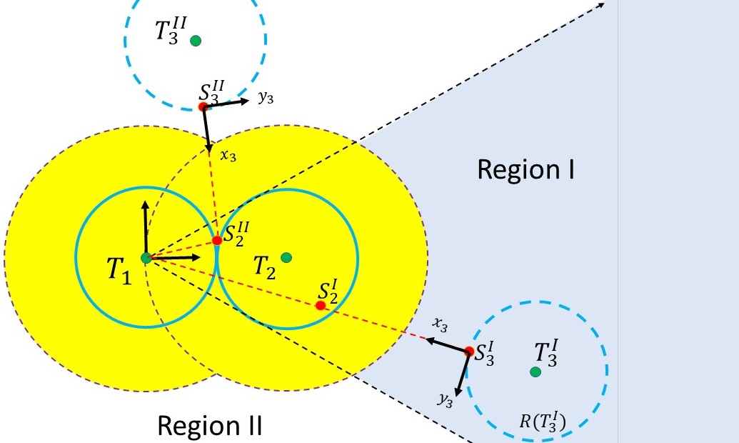
Case of One Active Constraint. We will next consider the cases where a single constraint is active (one pair of target nodes are separated by distance $2r$). There are three pairings to consider: $(R(T_{1}),R(T_{2}))$, $(R(T_{1}),R(T_{3}))$, and $(R(T_{2}),R(T_{3}))$. Figure 18 depicts the first constraint pairing, $(T_{1},T_{2})$. As in Figure 17, the problem is symmetric with respect to an axis passing through $T_{1}$ and $T_{2}$.

The KKT conditions under this constraint take the form:

$$\vec{0} \in \frac{\partial\mathcal{L}}{\partial T_{2}}\ \ \ \Rightarrow\ \ \ \vec{0}\ \in\ -\frac{\partial\Delta}{\partial T_{2}}-\lambda_{1,2}(T_{2}-T_{1})$$ (37)

$$\vec{0} \in \frac{\partial\mathcal{L}}{\partial T_{3}}\ \ \ \Rightarrow\ \ \ \vec{0}\ \in\ -\frac{\partial\Delta}{\partial T_{3}}$$ (38)

Using the same analysis of the three unconstrained targets in Figure 17, it is easy to see that in both Region I and Region II of Figure 18 that $\partial\Delta/\partial x_{3}$ is always positive, and therefore the KKT conditions cannot be satisfied in the interiors of Regions I and II. Moreover, for both regions, $\Delta$ is maximized on the boundary, where $||T_{3}-T_{2}||=2r$.

When $T_{1}$ and $T_{3}$ are constrained to be a distance $2r$ apart, the path passing through the sequence $T_{1}$-$T_{2}$-$T_{3}$ is not the shortest possible path through the targets – the visitation sequence must be reordered as $T_{1}$-$T_{3}$-$T_{2}$. This can be done by swapping the indices of $T_{2}$ and $T_{3}$. The newly relabeled problem thus has $T_{1}$ and $T_{2}$ constrained to be a distance $2r$ apart, and this case was analyzed above.

Figure 19: Geometry of $\mathcal{P}_{CPP}$ when $||T_{3}-T_{2}||=2r$.

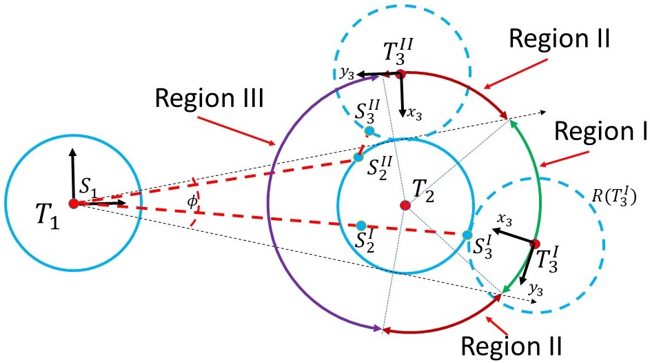
In the remaining single constraint case to consider, $T_{2}$ and $T_{3}$ lie a distance $2r$ apart (see Figure 19) so that target $T_{3}$ is constrained to lie on a circle of radius $2r$ centered on $T_{2}$. The KKT-conditions in this case are:

$$\vec{0} \in -\frac{\partial\Delta}{\partial T_{2}}+\lambda_{2,3}(T_{3}-T_{2})$$ (39)

$$\vec{0} \in -\frac{\partial\Delta}{\partial T_{3}}-\lambda_{2,3}(T_{3}-T_{2}).$$ (40)

As seen in Figure 19, the geometry of $\mathcal{P}_{CPP}$ changes as $T_{3}$’s location varies over the circle. In Region I of Fig. 19, $\mathcal{P}_{CPP}$ forms a straight line from $T_{1}$ that intersects the boundary of $R(T_{3})$ orthogonally. In Region II, $\mathcal{P}_{CPP}$ is a two segment path: the first segment connects $T_{1}$ to sensing location $S_{2}$, while the second segment departs $S_{2}$ and intersects the boundary of $R(T_{3})$ orthogonally at $S_{3}$. The location of $S_{2}$ is determined analogously to Equation (34). The character of $\mathcal{P}_{TSP}$ changes in Region III: the path sequence $T_{1}$-$T_{2}$-$T_{3}$ is not the shortest path through the targets, starting from $T_{1}$. As above, the indices of targets $T_{2}$ and $T_{3}$ are swapped to yield a correct path, resulting in a configuration that lies in either Region I or Region II. Thus, Region III can be ignored.

Let reference frame $\mathcal{F}_{3}$ be centered at $T_{3}$, with its $x$-axis colinear to $\overrightarrow{T_{3}T_{2}}$ (see Figure 19). For all locations of $T_{3}$ in Region I, the $y_{3}$ component of $\lambda_{2,3}(T_{3}-T_{2})$ in Equation (39) is zero. The magnitude of $l_{TSP}$ does not vary in Region I, and hence $\partial l_{TSP}/\partial y_{3}=0$. Consequently, the gradient of $\Delta$ simplifies to

$$\frac{\partial\Delta}{\partial x_{3}}=-(\frac{\Delta}{l_{CPP}})\frac{\partial l_{CPP}}{\partial x_{3}}.$$

This term take a nonzero value at all locations of $T_{3}$ except where $T_{1}$, $T_{2}$, and $T_{3}$ are colinear. Thus, the $y$-component of (40) is always nonzero, except at the colinear target condition. It can be shown that the colinear configuration is a saddle point. Thus, $\Delta$ is not extremized in Region I.

In Region II of Fig. 19, with $\mathcal{F}_{3}$ chosen as shown, the $y$-component of the term $\lambda_{23}(T_{3}-T_{2})$ is zero. But since $L_{CPP}$ varies as $T_{3}$ varies along Region II, Eq. (40) is not satisfied, and therefore there is no stationary point of $\Delta$ in Region II.

Case of Two Active Constraints. The are possible three groupings of paired constraints between sensing regions $R(T_{1})$, $R(T_{2})$, and $R(T_{3})$: $((R(T_{1}),R(T_{2}))\&(R(T_{2}),R(T_{3}))$; $((R(T_{1}),R(T_{3}))$ $\&$ $(R(T_{2}),R(T_{3})))$ and $((R(T_{1}),R(T_{2}))\&(R(T_{1}),R(T_{3})))$. Figure 20 depicts the geometry when constraints are active between $R(T_{1})$ and $R(T_{2})$, as well as $R(T_{2})$ and $R(T_{3})$. Different candidate locations of $T_{3}$ are shown.

Figure 20: Geometry of Sensing Regions and $\mathcal{P}_{CPP}$ when two constraints are active: $||T_{2}-T_{1}||=||T_{3}-T_{2}||=2r$. Three different configurations of $R(T_{3})$ are shown. Path $\mathcal{P}_{TSP}$ has the same length for all configurations. Path $\mathcal{P}_{CPP}$ (red dashed line) is shortest when the sensing regions form an equilateral triangle.

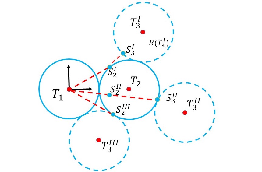
Note that $l_{TSP}$ is the same for all configurations of $T_{3}$ that satisfy the constraints. Hence, the ratio $\Delta$ is maximized when $\mathcal{P}_{CPP}$ achieves its shortest length. A direct calculation shows that $|\mathcal{P}_{CPP}|$ is minimized when the three sensing regions form a tightly nested equilateral triangle. An analogous result holds for the other constraint combinations.

In summary, the worst case ratio of the ratio $\Delta$ for the situation of 3 targets occurs when all inter-target constraints are active, resulting in a equilateral triangle configuration.

A-C Case of 4 Targets

Figure 21: Geometry of Sensing Regions and $\mathcal{P}_{CPP}$ for the case of 4 targets. (a) two constraints are active: $||T_{2}-T_{1}||=||T_{3}-T_{2}||=2r$, and $R(T_{4})$ is unconstrained. (b) Three different extremizing configurations of $R(T_{4})$ are shown.

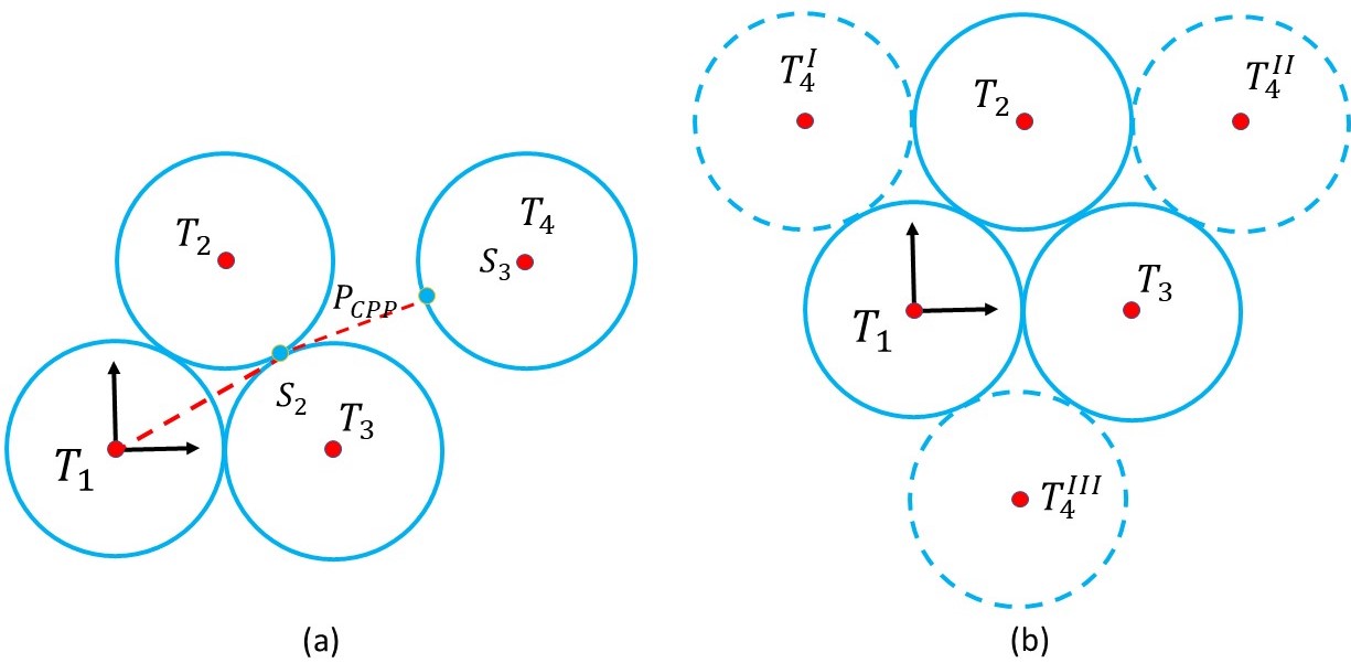
Figure 21(a) depicts a problem with 4 targets. The first three targets are constrained to form an equilateral triangle, with the fourth target placed at an arbitrary, but unconstrained, location. It can be shown, using the KKT-like analysis described above, that if targets $T_{2}$ or $T_{3}$ are displaced from their constrained configuration to a nearby unconstrained location, while the other targets remain fixed, then the value of $\Delta$ decreases. That is, targets $T_{2}$ and $T_{3}$ must be constrained as shown to maximize $\Delta$, regardless of the location of $T_{4}$. Again, using a KKT analysis, one can show that $\Delta$ is extremized when $R(T_{4})$ is constrained with respect to the other sensing regions. Figure 21 shows the three extremizing locations of target $T_{4}$, indicated by $T_{4}^{I}$, $T_{4}^{II}$, and $T_{4}^{III}$. A direct calculation shows that target location $T_{4}^{II}$ maximizes $\Delta$.

A-D Case of 5 and more targets

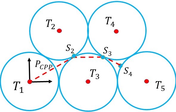
When a fifth target is added, the results above can be extrapolated to show that $\Delta$ is extremized when the sensing regions are tightly packed. Direct calculations show that maximum magnitude of $\Delta$ is realized in the configuration shown in Figure 22. For six or more targets, the same analytical approach leads to the linear packing arrangement of the sensing regions that is seen in Figure 5. As the number of targets increases, there are a discrete number of sensing circle packings that lead to the largest $\Delta$ ratio. However, the linear packing arrangement is as short as any other packing arrangment. Thus, the linear packing arrangement suffices for our analysis.

Figure 22: Extremizing Geometry of 5 Targets.

References

- [1] E. Acar, H. Choset, and J. Y. Lee. Sensor based coverage with extended range detectors. IEEE Transactions on Robotics, 22(1):189–198, 2006.
- [2] E. Acar, H. Choset, Y. Zhang, and M. Schervish. A survey on inspecting structures using robotic systems. Int. J. Robotics Research, 22:441–461, 2016.
- [3] Randa Almadhoun, Tarek Taha, Lakmal Seneviratne, Jorge Dias, and Guowei Cai. A survey on inspecting structures using robotic systems. Int. J. Advanced Robotics Systems, pages 1–18, 2016.
- [4] Pietro Belotti, Christian Kirches, Sven Leyffer, Jeff Linderoth, James Luedtke, and Ashutosh Mahajan. Mixed-integer nonlinear optimization. Acta Numerica, 22, 05 2013.
- [5] Andreas Bircher, Mina Kamel1, Kostas Alexis1, Michael Burri, Philipp Oettershagen1, Sammy Omari, Thomas Mantel1, and Roland Siegwart. Three-dimensional coverage path planning via viewpoint resampling and tour optimization for aerial robots. Autonomous Robots, 40:1059–1078, 2016.
- [6] R. Bland, D. Goldfarb, and M. Todd. The ellipsoid method: A survey. Operations Research, 29, 12 1981.
- [7] P. Bonami, L. T. Biegler, A. R. Conn, G. Cornuejols, I. E. Grossmann, C. D. Laird, A. Lodi J. Lee, F. Margot, and A. Waechter. An algorithmic framework for convex mixed integer nonlinear programs. Discrete Optimization, 5(2):186–204, 2008.
- [8] Joel W. Burdick, Amanda Bouman, and Elon Rimon. From multi-target sensory coverage to complete sensory coverage: An optimization-based robotic sensory coverage approach. In 2021 IEEE International Conference on Robotics and Automation (ICRA), pages 10994–11000, 2021.
- [9] Christofides, N. Worst-Case analysis of a new heuristic for the travelling salesman problem. Technical Report 388, Carnegie-Mellon University, Pittsburgh, PA, 1976.
- [10] Walton Pereira Coutinho, Roberto Quirino do Nascimento, Artur Alves Pessoa, and Anand Subramanian. A Branch-and-Bound Algorithm for the Close-Enough Traveling Salesman Problem. INFORMS Journal on Computing, 28(4):752–765, November 2016.
- [11] John R. Current and David A. Schilling. The Covering Salesman Problem. Transportation Science, 23(3):208–213, August 1989.
- [12] T. Danner and L.E. Kavraki. Randomized planning for short inspection paths. In IEEE Int. Conf. on Robotics and Automation, pages 971–976 vol.2, San Francisco, CA, USA, 2000. IEEE.
- [13] Adrian Dumitrescu and Joseph S B Mitchell. Approximation algorithms for TSP with neighborhoods in the plane. Journal of Algorithms, 48(1):135–159, 2003.
- [14] Brendan Englot and Franz Hover. Planning Complex Inspection Tasks Using Redundant Roadmaps. In Henrik I. Christensen and Oussama Khatib, editors, Robotics Research, volume 100, pages 327–343. Springer International Publishing, Cham, 2017.
- [15] Brendan Englot and Franz S. Hover. Three-dimensional coverage planning for an underwater inspection robot. Int. J. Robotics Research, 32(9-10):1048–1073, August 2013.
- [16] E. Galceran and M. Carrares. Efficient seabed coverage path planning for asvs and auvs. In IEEE/RSJ Int. Conf. on Intelligent Robots and Systems, pages 88–93, 2012.
- [17] E. Galceran and M. Carreras. A survey on coverage path planning for robotics. Robotics and Autonomous Systems, 61(4):146–155, 2013.
- [18] Iacopo Gentilini, François Margot, and Kenji Shimada. The travelling salesman problem with neighbourhoods: MINLP solution. Optimization Methods and Software, 28(2):364–378, April 2013.
- [19] Bruce Golden, Zahra Naji-Azimi, S. Raghavan, Majid Salari, and Paolo Toth. The Generalized Covering Salesman Problem. INFORMS Journal on Computing, 24(4):534–553, November 2012.
- [20] Michael Grant and Stephen Boyd. Graph implementations for nonsmooth convex programs. In V. Blondel, S. Boyd, and H. Kimura, editors, Recent Advances in Learning and Control, Lecture Notes in Control and Information Sciences, pages 95–110. Springer-Verlag Limited, 2008. http://stanford.edu/~boyd/graph_dcp.html.
- [21] Michael Grant and Stephen Boyd. CVX: Matlab software for disciplined convex programming, version 2.1. https://cvxr.com/cvx, March 2014.
- [22] J.A. Hoogeveen. Analysis of Christofides’s heuristic: Some paths are more difficult than cycles. Operat. Res. Lett., 10:291–295, 1991.
- [23] Inverse Problem Limited. Opti Toolbox - A Free Matlab Tool for Optimization . https://www.inverseproblem.co.nz/OPTI/, 2019.
- [24] Donald B. Johnson. Efficient algorithms for shortest paths in sparse networks. J. ACM, 24(1):1–13, jan 1977.
- [25] S Kapoor, S N Maheshwari, and J S B Mitchell. An efficient algorithm for euclidean shortest paths among polygonal obstacles in the plane. Discrete & Computational Geometry, 18(4):377–383, December 1997.
- [26] Vladimir Kolmogorov. Blossom V: a new implementation of a minimum cost perfect matching algorithm. Mathematical Programming Computation, 1(1):43–67, July 2009.
- [27] J. Kronqvist, D. Bernal, A. Lundell, and I. Grossmann. A review and comparison of solvers for convex MINLP. Optimization and Engineering, 20, 06 2019.
- [28] Helge A. Lauterbach, C. Bertram Koch, Robin Hess, Daniel Eck, Klaus Schilling, and Andreas Nuchter. The Eins3D project — Instantaneous UAV-Based 3D Mapping for Search and Rescue Applications. In IEEE Int Symp Safety, Security, and Rescue Robotics, pages 1–6, Würzburg, Germany, September 2019. IEEE.
- [29] S. G. Loizou and C. C. Constantinou. Multi-robot coverage on dendritic topologies under communication constraints. In IEEE 55th Conference on Decision and Control, pages 43–48, 2016.
- [30] T. Marcussi, M. Petersen, D. Wrangel, and R. Tedrake. Motion planning around obstacles with convex optimization. arXiv:2205.04422, May 2022.
- [31] Joseph S.B. Mitchell, Csaba D. Tóth, Jacob E. Goodman, and Joseph O’Rourke. Shortest paths and networks. Chapman & Hall/CRC, 3rd edition, 2017.
- [32] Patrick A Plonski and Volkan Isler. Approximation algorithms for tours of height-varying view cones. The International Journal of Robotics Research, 38(2-3):224–235, 2019.
- [33] F.P. Preparata and M.I. Shamos. Computational Geometry: An Introduction. Monographs in Computer Science. Springer New York, 2012.
- [34] Michael Ian Shamos and Dan Hoey. Geometric intersection problems. In 17th Annual Symposium on Foundations of Computer Science (sfcs 1976), pages 208–215, 1976.
- [35] Pratap Tokekar, Joshua Vander Hook, David Mulla, and Volkan Isler. Sensor Planning for a Symbiotic UAV and UGV System for Precision Agriculture. IEEE Transactions on Robotics, 32(6):1498–1511, December 2016.
- [36] A. Vecchietti, S. Lee, and I.E. Grossman. Modeling of Discrete/Continuous Optimization Problems: Characterization and Formulation of Disjunctions and Their Relaxations. Computers and Chemical Engineering, 27(3):433–448, 2003.
- [37] Emo Welzl. Constructing the visibility graph for n-line segments in o(n2) time. Information Processing Letters, 20(4):167–171, 1985.
- [38] D. P. Williamson and D. B. Shmoys. The Design of Approximation Algorithms. Cambridge University Press, N.Y., 2011.