Stability analysis of nonlinear stochastic flexibility function in smart energy systems

Abstract

Demand-side management provides a great potential for improving the efficiency and reliability of energy systems. This requires a mechanism to connect the market level and the demand side. The flexibility function is a novel approach that bridges the gap between the markets and the dynamics of physical assets at the lower levels of the energy systems and activates demand-side flexibility with the purpose of decision-making as well as for offering a new framework for balancing and grid services. Employing this function as a key for many decision-making and control algorithms reveals that a mathematically rigorous stability analysis is required for it. In this paper, we investigate the stability properties of two nonlinear flexibility functions, as a dynamic mapping between electricity price and power consumption. Specifically, we analyze the stability of a deterministic flexibility function and an Itô stochastic flexibility function. Simulation results are also provided to demonstrate the dynamics of the flexibility functions and to show that the analytical results hold.

, , , ,

1 Introduction

Decarbonization of the energy system forms an immense priority towards the reduction of the rate of global warming [1]. Thereupon, energy systems worldwide are now subject to ambitious goals regarding penetration levels of renewable energy sources (RES). Such developments, however, challenge the traditional operations of power systems, where the supply side is controlled to meet the inflexible demand and call for control capabilities on the demand side for the latter to meet the intermittent renewable supply [2], [3], [4].

This paradigm shift brings about the development of control and communication capabilities toward harvesting the innate flexibility of existing electricity loads. This has led to an outburst of research studies for demand-side energy management, spanning different types of loads (e.g. residential [5], industrial [6], cross-sector [7]) and methodological approaches (e.g. optimization [8], control [9], artificial intelligence [10]). A characteristic example refers to the management of thermostatically controlled loads to offer load-shifting services by leveraging the natural thermal storage capability of the building envelope [11], [12], [13].

The multitude of small, demand-side resources along with their different characteristics and their heterogeneous control methods constitutes a major barrier towards their coordination and integration into hierarchical control [14], [15], [16] or market [17], [18], [19] frameworks. A prominent approach towards achieving scalable coordination frameworks for flexible electricity loads refers to the so-called “transactive control” paradigm [20], which constitutes a market-based hierarchical control method, where a resource’s controller receives a set of prices (communicated by an upstream controller) and adapts its consumption profile as a response to these prices considering also its internal state and characteristics.

From a practical perspective, however, it remains an open challenge to integrate heterogeneous resource-level controllers into an upstream coordination framework that also considers uncertainty and schedules operations for times ahead. A solution to this problem is to capture a resource’s (e.g. building’s) flexibility capabilities into a generic grey-box model [21] that can be used seamlessly in upstream control or market frameworks [22]. Such a model is instantiated in [23] as a set of stochastic differential equations that provide a nonlinear mapping between a set of electricity prices (for a look-ahead horizon) and a resource’s power consumption profile that comes as a response to those prices, and coined as a resource’s “Flexibility Function”. As further showcased in [23], [24], and [25], by simply tuning the parameters of the Flexibility Function, we can use it to capture the price-consumption behavior of different types of loads and their respective controllers. This offers great potential towards a seamless integration of distributed flexibility capabilities and it is currently considered as a cornerstone of minimum interoperability mechanisms for a smart operating system under development by the Danish power system operator.

Stability analysis of the energy system and controller design are investigated in many research articles. For instance, the stability of the energy system considering dynamic-pricing controllers and distributed control architecture are discussed in [26] and [3], respectively. To enable the adoption of the Flexibility Function as a standard in real systems, it is of prominent importance that the model that instantiates a resource’s Flexibility Function is theoretically proven to be stable, i.e., it always provides a meaningful output of the resource’s expected consumption profile once provided with a set of prices. This motivates the main contribution of this paper, which is to identify the region of the Flexibility Function’s parameters, within which the model remains stable. Specifically, the stability of a deterministic Flexibility Function and an Itô [27] stochastic Flexibility Function is analyzed. This provides a solid theoretical foundation for the model’s use in the critical domain of power systems, while also providing a practical tool for ensuring that the tuning of the Flexibility Function upon modeling any particular resource stays within a meaningful and well-behaved region. The other contribution of this study is to translate the flexibility function into an input-state-output form, which allows it to fit into the standard paradigm for systems theory. To the best of our knowledge, such a result is not available in the prior literature. This approach makes use of concepts such as equilibrium points, stability, and boundedness, which in turn simplifies the analysis of flexibility dynamics.

This paper is organized as follows: Section 2 gives an overview of the Flexibility Function. Sections 3 and 4 provide the stability analysis of the deterministic and stochastic Flexibility Functions, respectively. Section 5 demonstrates the simulation results to demonstrate stability analysis results. Finally, a summary is given in Section 6.

1.1 Notation

In this paper, $\mathbb{R}$ denotes the set of real numbers. Elements of a set can be provided using $\{.\}$. Closed interval is shown as $[a,b]=\{x\in\mathbb{R}|a\leq x\leq b\}$. The symbol $/$ is used for set subtraction. The symbol $\wedge$ stands for the logical and, i.e., $a\wedge b$ is true if both $a$ and $b$ are true. $\Pr(.)$ and $E[.]$ denote probability and expected value, respectively. Also, the normal distribution with a mean of $\mu$ and a standard deviation of $\sigma$ is denoted by $N(\mu,\sigma)$. If $X$ has normal distribution, we write $X\sim N(\mu,\sigma)$. Moreover, $C^{2}$ stands for twice continuously differentiable, and $tr(.)$ refers to the trace operation. $\vmathbb{1}_{q}$ is the indicator function, i.e., it is equal to one only if the logic $q$ is true. Finally, $||.||$ is the $L_{2}$ norm and $|c|$ is the absolute value of $c\in\mathbb{R}$.

2 Flexibility Function

Flexibility is the capability of adjusting the energy demand profile according to climate conditions, grid requirements, and comfort constraints. Energy systems have the flexibility potential. Exploiting this potential is a key task for energy management and load scheduling in modern energy systems. Lack of predictability on the demand side raises the need for a systematic way to represent the flexibility potential and predict it. Flexibility function is a dynamical system that introduces a linkage between demand, state of charge, and price [22].

The nonlinear dynamics of the price-demand relationship, as proposed in [23], is in the following stochastic differential equation form. The dynamics of the state of charge of flexibility function is

$$d{\mathcal{X}}_{t} =\frac{1}{C}\Delta D_{t}dt+\mathcal{X}_{t}(1-\mathcal{X}_{t})\sigma_{x}dW_{t},$$ (1)

where $\mathcal{X}\in[0,\ 1]\subset\mathbb{R}$ is the state of charge, $C\in\mathbb{R}^{+}$ is the capacity of flexible energy, $\sigma_{X}$ represents process noise intensity, and $W$ is a Wiener process. It is seen that positive $\Delta D_{t}$ leads to an increase in $\mathcal{X}_{t}$ and ultimately reduces the diffusion. On the contrary, if $\Delta D_{t}$ is negative, $\mathcal{X}_{t}$ reduces and ultimately reduces the diffusion. Furthermore, $\Delta D\in[-1,\ 1]\subset\mathbb{R}$ is defined as the following function,

$$\Delta D_{t}=\begin{cases}\delta_{t}\lambda(1-B_{t}),&\text{ if}\ \ \delta_{t}\geq 0,\\ \delta_{t}\lambda B_{t},&\text{ if}\ \ \delta_{t}<0,\end{cases}$$ (2)

where $B_{t}\in[0,\ 1]\subset\mathbb{R}$ is the baseline demand, $\lambda\in(0,\ 1)\subset\mathbb{R}$ is the portion of the demand and $\delta_{t}$ is the demand change. If $\delta_{t}$ is positive, i.e., the state of charge is increasing, then, $\Delta D_{t}$ is equal to $\delta_{t}$ multiplied by a portion of the difference between full demand and the baseline demand $(1-B_{t})$. Otherwise, $\Delta D_{t}$ is equal to $\delta_{t}$ multiplied by a portion of the difference between the null demand and the baseline demand $(B_{t})$. $\Delta D_{t}$ can be interpreted as the deviation of the predicted demand from the baseline demand as

$$D_{t}=B_{t}+\Delta D_{t},$$ (3)

where $D_{t}[0,\ 1]\subset\mathbb{R}$ is the predicted demand that can be considered as the flexibility function output.

The nonlinear function defining $\delta_{t}$ is a logistic function of $\mathcal{X}_{t}$ and the price $(u_{t})$ as:

$$\ell(z_{t}) =-1+\frac{2}{1+e^{-kz_{t}}},$$ (4)

where $z_{t}\equiv f(\mathcal{X}_{t})+g(u_{t})$, where $f(.)\in[-1,\ 1]$ is a polynomial function between the state of charge and energy demand and $g(.)\in[-1,\ 1]$ is a summation of I-splines representing the relation between the energy price and energy demand [28] as

$$g(u_{t}) =\beta_{1}I_{s,1}(u_{t})+...+\beta_{7}I_{s,7}(u_{t}),$$ (5)

$$f(\mathcal{X}_{t}) =\left(1-2\mathcal{X}_{t}+\alpha_{1}\left(1-(2\mathcal{X}_{t}-1)^{2}\right)\right)$$

$$\times\left(\alpha_{2}+\alpha_{3}(2\mathcal{X}_{t}-1)^{2}+\alpha_{4}(2\mathcal{X}_{t}-1)^{6}\right),$$ (6)

where $I_{s,1}$, …, $I_{s,7}$ are I-spline functions , $\beta_{1},...,\beta_{7}$, $\alpha_{1},...,\alpha_{4}$, and $k$ are parameters to be identified. These parameters can be identified using different approaches to maximize the likelihood between the final flexibility function and the data. The following two remarks reveal some useful aspects of determining $f(.)$ and $g(.)$.

Remark 1.

The following three concepts form the basis of the flexibility function dynamics: 1) high prices lead to a reduction in demand, while low prices tend to increase demand, 2) more stored energy leads to a reduction in demand, while less stored energy tends to increase demand, and 3) the energy storage capacity is finite. As a result of the first two concepts, the functions $f(.)$ and $g(.)$ are determined such that they are monotonically decreasing. Furthermore, the function $\ell(.)$, mapping $f(.)+g(.)$ to the interval $(0,1)$ is designed to be monotonically increasing, which represents the effect of having low/high price and low/high state of charge at the same time (see Figure 1).

Remark 2.

The functions $f(.)$ and $g(.)$ are selected in a way that $f(1)+g(u)\leq 0$ and $f(0)+g(u)\geq 0$ for all $u\in[0,\ 1]$. Considering that $u=1$ minimizes $g(u)$, and $u=0$ maximizes it, $f(.)$ and $g(.)$ are chosen such that $f(1)+g(0)=0$ and $f(0)+g(1)=0$ (see Figure 1).

In the following, we first disregard the stochastic terms in (1) and investigate the stability of the deterministic flexibility function. Then, we analyze the stochastic dynamics of (1) as a general model for demand-response dynamics.

3 Stability Analysis of the Deterministic Flexibility Function

Disregarding the diffusion part of the flexibility function provides a clarified overview of the demand-response behavior. This simplified ordinary differential equation helps us understand the core of its dynamics and can be viewed as an introduction to a more complex stochastic flexibility function. Other studies like [29] have utilized this simplified flexibility function as a price-demand relationship. To this end, the flexibility function can be written as

$$d{\mathcal{X}}_{t}/dt =\frac{1}{C}\Delta D_{t},$$ (7)

$$\Delta D_{t} =\begin{cases}\delta_{t}\lambda(1-B_{t}),&\text{ if}\ \ \delta_{t}\geq 0,\\ \delta_{t}\lambda B_{t},&\text{ if}\ \ \delta_{t}<0,\end{cases},$$ (8)

$$D_{t} =B_{t}+\Delta D_{t},$$ (9)

$$\delta_{t} =\ell(z_{t}),$$ (10)

$$z_{t} =f(\mathcal{X}_{t})+g(u_{t}),$$ (11)

for the further analysis. In the following, we first investigate the flexibility function by finding equilibrium points of it, and then analyze its stability using Lyapunov stability analysis.

3.1 Set invariance property

In this subsection, we show that the flexibility function (7)-(11) has the property to keep the state of charge in the range $[0,\ 1]$. Specifically, we validate the flexibility function at $\mathcal{X}_{0}=1$ and $\mathcal{X}_{0}=0$.

Suppose that the price is $\bar{u}$, the baseline demand is $\bar{B}\in(0,\ 1)$, and $\mathcal{X}_{0}=1$. Then, using the properties of $f(.)$ and $g(.)$, introduced in Remark 1 and 2, it implies that $f(\mathcal{X}_{0})=-1$, which leads to $f(\mathcal{X}_{0})+g(\bar{u})<0$. Consequently, from (11), (10) and (8), it can be obtained that $z<0$, $\delta<0$, and $\Delta D<0$. This shows that $d{\mathcal{X}}_{t}/dt<0$, and proves that $\mathcal{X}$ will not leave the set $[0,\ 1]$. The same argument holds for the price $\bar{u}$, the baseline demand $\bar{B}\in(0,\ 1)$, and $\mathcal{X}_{0}=0$. One can show that $d{\mathcal{X}}_{t}/dt>0$, which proves that $\mathcal{X}$ will not leave the set $[0,\ 1]$.

3.2 Equilibrium points

Equilibrium points are crucial in determining the stability and convergence properties of a dynamic system. They play a significant role in stability theorems by helping to investigate the behavior of the system in the vicinity of the equilibrium points. Therefore, it is important to understand the concept of equilibrium points when analyzing the stability of a dynamic system.

The equilibrium points of the system are the points that make the right-hand side of (7) equal to zero, that is, $\Delta D_{t}=0$. Hence, once demand matches the baseline, the dynamics of the flexibility function are in equilibrium. Considering (8), this happens when $\delta_{t}=0$ or equivalently, $\ell(f(\mathcal{X}_{t})+g(u_{t}))=0$. Thus, the set consisting the equilibrium point(s), $X^{*}$, of the system can be defined as

$$\Omega=\{(X^{*},u^{*})|f({\mathcal{X}})=-g(u^{*})\}$$ (12)

for the specified $u^{*}$ and $B^{*}$. It is noted that since there exists a unique $u^{*}$ corresponding to each $\mathcal{X}$ (see Remark 1 and 2), we denote the equilibrium points as a pair, $(X^{*},u^{*})$.

Remark 3.

One may also ask about other points that make the right-hand side of (7) equal to zero. These points are related to the extremum values of the baseline signal. It is seen in (8) that $\Delta D_{t}$ is equal to zero when $B_{t}=0$ and $\delta_{t}<0$, or $B_{t}=1$ and $\delta_{t}\geq 0$. Although this proposition may look correct, by looking in more detail it reveals that it is not physically meaningful. When, $B_{t}=0$, $D_{t}$ is greater or equal to zero, leading to $\delta_{t}\geq 0$. This is the same for $B_{t}=1$. When, $B_{t}=1$, $D_{t}$ is less than or equal to $1$, leading to $\delta_{t}\leq 0$.

To simplify the stability analysis, one can, without loss of generality, apply a change of variable, and investigate the stability around the origin. The transformed system is written as:

$$\frac{d{\mathfrak{X}}_{t}}{dt} =\frac{1}{C}\Delta D_{t},$$ (13)

$$\Delta D_{t} =\begin{cases}\delta_{t}\lambda(1-B_{t}),&\text{ if}\ \ \delta_{t}\geq 0,\\ \delta_{t}\lambda B_{t},&\text{ if}\ \ \delta_{t}<0,\end{cases},$$ (14)

$$D_{t} =B_{t}+\Delta D_{t},$$ (15)

$$\delta_{t} =\ell(z_{t}),$$ (16)

$$z_{t} =f(\mathfrak{X}_{t}+X^{*})+g(u_{t}),$$ (17)

where $\mathfrak{X}=\mathcal{X}-X^{*}$, $X^{*}\in\Omega$. The equilibrium point of the transformed system is at 0. In the sequel, we analyze the stability of the dynamics (13)-(17).

3.3 Stability analysis of the equilibrium points

This section is dedicated to the stability analysis of the equilibrium points of the flexibility function, disregarding the stochasticity, using Lyapunov stability theorem [30].

Theorem 1 Consider the transformed flexibility function (13)-(17) and let $\mathbb{D}$ be a domain containing the origin. Then given any initial condition in $\mathbb{D}$, and any $u^{*}\in[0,\ 1]$ and $B^{*}\in[0,\ 1]$, the equilibrium point of (13)-(17) is asymptotically stable.

Proof Consider the Lyapunov function candidate $V(\mathfrak{X}_{t})=\frac{1}{2}\mathfrak{X}_{t}^{2}$. If one can show that $\frac{d}{dt}V(\mathfrak{X}_{t})<0$ for $\mathfrak{X}_{t}\neq 0$, then the stability of the equilibrium point is guaranteed. The time derivative of $V$ along the trajectories of $\mathfrak{X}_{t}$ can be calculated as

$$\frac{d}{dt}V(\mathfrak{X}_{t})=\mathfrak{X}_{t}\frac{d}{dt}\mathfrak{X}_{t}=\frac{1}{C}\Delta D_{t}\mathfrak{X}_{t}.$$ (18)

Considering $u_{t}=u^{*}$ and $B_{t}=B^{*}$, and substituting (14), (18) can be rewritten as

$$\frac{d}{dt}V(\mathfrak{X}_{t}) =\begin{cases}\frac{1}{C}\mathfrak{X}_{t}\delta_{t}\lambda(1-B_{t}),&\text{ if}\ \ \delta_{t}\geq 0,\\ \frac{1}{C}\mathfrak{X}_{t}\delta_{t}\lambda B_{t},&\text{ if}\ \ \delta_{t}<0,\end{cases}.$$ (19)

By utilizing Remark 1 and the monotonicity of $f(.)$, $f(\mathcal{X})+g(u^{*})>0$ implies $\mathcal{X}<X^{*}$ and $f(\mathcal{X})+g(u^{*})<0$ implies $\mathcal{X}>X^{*}$, for $X^{*}\in\Omega$. The following two cases should be considered, 1) $\delta_{t}>0$, $X^{*}\in\Omega$, and 2) $\delta_{t}<0$, $X^{*}\in\Omega$:
Case 1:
This case considers $\delta_{t}>0$ which leads to $\Delta D_{t}>0$. Thus, $\mathfrak{X}_{t}$ increases while $\mathfrak{X}_{t}<0$. Therefore, $\mathfrak{X}_{t}$ converges to $0$, that is, $\mathcal{X}_{t}$ reaches $X^{*}$.
Case 2:
This case considers $\delta_{t}<0$ which leads to $\Delta D_{t}<0$. Thus, $\mathfrak{X}_{t}$ decreases while $\mathfrak{X}_{t}>0$. Therefore, $\mathfrak{X}_{t}$ converges to $0$, that is, $\mathcal{X}_{t}$ reaches $X^{*}$.

Considering the above cases, when $\delta_{t}>0$, $\mathfrak{X}_{t}$ is negative and when $\delta_{t}<0$, $\mathfrak{X}_{t}$ is positive. Figure 1 demonstrates the above cases. Therefore, with the above-mentioned results and (19), it can be implied that $\frac{d}{dt}V(\mathfrak{X}_{t})<0$ for all $\mathfrak{X}_{t}\in\mathbb{D}\setminus\{0\}$, which proves the asymptotic stability of the equilibrium point. It is noted that $\Delta D_{t}=0$ corresponds to the case when the flexibility dynamics are at the equilibrium, that is, $\mathfrak{X}_{t}=0$. ∎

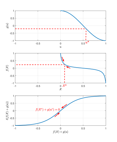
Figure 1: Schematic of nonlinear functions of the flexibility function for the stability analysis. The functions $f$ and $g$ are selected to demonstrate the analysis.

3.4 Simulation results

Figure 2 demonstrates the simulation results of the deterministic flexibility function concerning changes in initial state, price, and baseline values. The top panel of this figure illustrates the states of charge considering different initial conditions in the range $[0,\ 1]$, while price and baseline are fixed at $u=0.5$ and $B=0.4$, respectively. It is seen that the state of charge remains stable and the trajectories converge to the equilibrium point of the system for any initial state. The next panel of Figure 2 shows the state of charge for changing prices, while the initial state and baseline are constant values as $\mathcal{X}_{0}$ and $B=0.4$. It is observed that the state is bounded and converges to steady-state values. Low prices lead to a higher state of charge steady-state while the elevation of prices lowers its steady-state. The bottom panel of Figure 2 depicts the state of charge concerning the baseline signal altering. It is seen that the trajectories converge to the different equilibrium points due to changes in $B$. Increasing the baseline increases the rate of change of state of charge. This fact can also be manifested from (13).

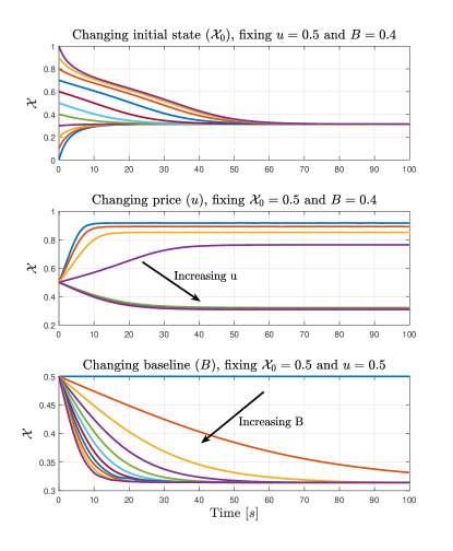
Figure 2: Trajectories of state of charge, based on changes in initial state, price, and baseline.

4 Stochastic Stability Analysis

Stochastic differential equations are an appropriate approach for modeling physical, biological, and economical dynamical systems with significant uncertainty and where the future values of the states cannot be predicted exactly. The generalized flexibility function is modeled as a stochastic differential equation and consists of both the deterministic part, which is investigated in Section 2, and the stochastic part. The stochasticity enables the generalized flexibility function to predict the price-demand relationships realistically. Thus, employing this function in a smart energy Operating System enhances the performance of control and decision-making algorithms. This shows the significance of stability analysis of the stochastic price-demand mapping.

We first show the importance of the stochastic stability analysis using the following three examples [31].

Example 4.

Consider the following bilinear scalar dynamical system

$$\dot{x}(t)=r_{1}x(t)+r_{2}x(t)w(t).$$ (20)

For a deterministic $w(t)$, $r_{1}+r_{2}w(t)$ determines the stability properties of this system. Considering the Lyapunov function $x^{2}/2$, it is simple to show that (20) is stable if $r_{1}+r_{2}w(t)$ is negative for all $t$.

Example 5.

For a stochastic input $w(t)$, independent of $x(t)$, expectation of both sides of (20) can be written as

$$\frac{d}{dt}E[x(t)] =(r_{1}+r_{2}\omega_{t})E[x(t)],$$ (21)

where $\omega_{t}$ is the mean value of $w(t)$. Using the same discussion as the deterministic input with Lyapunov function $E[x]^{2}/2$, it can be proven that (21) is stable if $r_{1}+r_{2}\omega_{t}$ is nonpositive for $\forall t$. However, this is not the case for Itô stochastic differential equations.

Example 6.

Consider the Itô stochastic differential equation [27]

$$dx(t)=r_{1}x(t)dt+r_{2}x(t)dw(t),$$ (22)

where $w(t)$ is a Brownian motion. The explicit solution of (22) can be found as $x(t)=x(t_{0})e^{(r_{1}-0.5r_{2}^{2})t+r_{2}w(t)}$ [27]. This reveals that $x(t)$ is bounded if $r_{1}-r_{2}^{2}/2\leq 0$ and converges to zero if $r_{1}-r_{2}^{2}/2<0$.

Figure 3 shows the simulation results for the above three examples. This figure shows the difference in the stability properties of seemingly similar systems in Example 1-3. While the systems of Example 1-2 are stable with $r_{1}=1$ and $r_{2}=-1.2$, the stochastic differential equation (Example 3) with similar $r_{1}$ and $r_{2}$ diverges. On the contrary, with $r_{1}=1$ and $r_{2}=2$, the stochastic differential equation of Example 3 converges to zero as time reaches infinity, while systems of Example 1-2 have unstable behaviors.

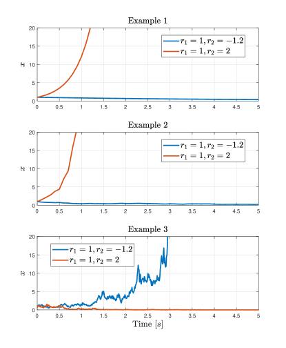
Figure 3: State trajectories of the systems in Example 1-3.

Before moving toward the stochastic stability analysis of the flexibility function, we should investigate its equilibrium points. Equilibrium points of the stochastic flexibility function (1)-(6), are the points at which, $\frac{1}{C}(D_{t}-B_{t})=0$ and $\mathcal{X}_{t}(1-\mathcal{X}_{t})\sigma_{x}=0$. Since $\mathcal{X}_{t}(1-\mathcal{X}_{t})\sigma_{x}=0$ only at $\mathcal{X}=0$ and $\mathcal{X}=1$, the set of equilibrium points of the stochastic flexibility function can be found as

$$\Omega_{s}=\{(\mathcal{X},u^{*})|\mathcal{X}\in\{0,\ 1\}\wedge(\mathcal{X},u^{*})\in\Omega\},$$ (23)

where $\Omega$ is defined in (12). Hence, $\Omega_{s}=\{(0,\ 1),\ (1,\ 0)\}$. In the sequel, we analyze the stability of the equilibrium points of the stochastic flexibility function.

4.1 Stochastic stability of flexibility function

In general, finding an explicit expression for the solution of a system of stochastic differential equations is impossible. However, through a stochastic stability analysis, we can derive a characterization of the behaviors of the solutions. We start the investigation by introducing the main definitions and theorems for the stochastic stability analysis.

Definition 1.

[32] The solution $X_{t}$ of the stochastic differential equation $dX_{t}=f(X_{t})dt+g(X_{t})dB_{t}$ with equilibrium $X^{*}$ is stochastically stable (stable with probability one) if for every $\epsilon>0$, there exists a $\delta>0$ so that if $||X_{t_{0}}-X^{*}||<\delta$, then

$$\lim_{X_{t_{0}}\rightarrow X^{*}}\Pr\left(\sup_{t\geq t_{0}}||X_{t}-X^{*}||\geq\epsilon\right)=0.$$ (24)

Definition 2.

[33] The differential operator $\mathcal{L}$ on function $V(X_{t})$ in $C^{2}$ is defined as

$$\mathcal{L}V(X_{t})=\frac{d}{dX}Vf(X_{t})+\frac{1}{2}\text{tr}\left(g(X_{t})^{T}\frac{d^{2}V(X_{t})}{dX^{2}}g(X_{t})\right)$$ (25)

where the dynamics of $X_{t}$ follows the stochastic differential equation $dX_{t}=f(X_{t})dt+g(X_{t})dB_{t}$.

Theorem 2[34] Let $X^{*}$ be an equilibrium point of the stochastic differential equation $dX_{t}=f(X_{t})dt+g(X_{t})dB_{t}$. Suppose that there exists a function $V$ defined on the domain $\hat{\mathbb{D}}$, containing $X^{*}$, such that:
1) $V$ is $C^{2}$ on $\hat{\mathbb{D}}\setminus{{X}^{*}}$,
2) There exist positive definite functions $k_{1}$ and $k_{2}$, such that $k_{1}(|X-X^{*}|)\leq V(X)\leq k_{2}(|X-X^{*}|)$,
3) $\mathcal{L}V(X)\leq 0$ for $|X-X^{*}|\geq K$ with some constant $K$.
Then, the solution of the stochastic differential equation is stochastically bounded around $X^{*}$, that is, for each $\epsilon>0$, there exists a $\rho$ such that

$$\Pr\left(\sup_{t\geq t_{0}}||X_{t}-X^{*}||\leq\epsilon\right)>1-\rho.$$ (26)

Theorem 3 [27] Let $X^{*}$ be an equilibrium point of the stochastic differential equation $dX_{t}=f(X_{t})dt+g(X_{t})dB_{t}$. Suppose that there exists a function $V$ defined on the domain $\hat{\mathbb{D}}$, containing $X^{*}$, such that the first and second conditions of Theorem 4.1 are satisfied and $\mathcal{L}V(X)\leq 0$ for $X\in\hat{\mathbb{D}}\setminus{{X}^{*}}$. Then, the solution of the stochastic differential equation is stochastically stable.

After discussing the importance of stochastic stability analysis for the stochastic differential equation, and providing the required definitions and theorems in this regard, it is time to investigate the boundedness and stability of the solutions of the stochastic flexibility function, given in (1)-(6).

Theorem 4 Let $(X^{*},u^{*})\in\Omega_{s}$ be an equilibrium point of the stochastic flexibility function (1-6). Then given any initial condition, $X_{t_{0}}$, in $\mathbb{D}$, and any $B^{*}\in[0,\ 1]$, $C$, and $\Delta$, and $u^{*}\in\{0,\ 1\}$, there exist $\sigma>0$ such that for $\sigma_{x}\in[0,\ \sigma]$, the equilibrium points of (1)-(6) are stochastically bounded.

Proof Consider the candidate function $V(\mathcal{X}_{t})=\frac{1}{2}(\mathcal{X}_{t}-X^{*})^{2}$ which is $C^{2}$ on ${\mathbb{D}}\setminus{{X}^{*}}$. It can be shown that there exist positive definite functions $k_{1}=c_{1}(\mathcal{X}_{t}-X^{*})^{2}$ and $k_{2}=c_{2}(\mathcal{X}_{t}-X^{*})^{2}$, with $0<c_{1}<0.5$ and $0.5<c_{2}$ such that $k_{1}\leq V\leq k_{2}$. Furthermore,

$$\mathcal{L}V(\mathcal{X})=\frac{1}{C}(D_{t}-B_{t})(\mathcal{X}-X^{*})+\frac{1}{2}\mathcal{X}^{2}(1-\mathcal{X})^{2}\sigma_{x}^{2}$$

$$=\frac{\Delta}{C}\ell(f(\mathcal{X}_{t},\alpha)+g(u_{t},\beta),k)(\vmathbb{1}_{\delta_{t}>0}(1-B_{t})+\vmathbb{1}_{\delta_{t}<0}B_{t})$$

$$\times(\mathcal{X}-X^{*})+\frac{1}{2}\mathcal{X}^{2}(1-\mathcal{X})^{2}\sigma_{x}^{2},$$ (27)

that consists of two terms. The first term is $\eta\ell(f(\mathcal{X}_{t},\alpha)+g(u_{t},\beta),k)(\mathcal{X}-X^{*})$, with $\eta\coloneqq\frac{\Delta}{C}(\vmathbb{1}_{\delta_{t}>0}(1-B_{t})+\vmathbb{1}_{\delta_{t}<0}B_{t})$, and the second term is $\frac{1}{2}\mathcal{X}^{2}(1-\mathcal{X})^{2}\sigma_{x}^{2}$. It is noted that the second term is always positive for $\mathcal{X}\in{\mathbb{D}}\setminus{{X}^{*}}$ and $\eta$ is a positive value. In the sequel, we first show that the first term is negative and then complete the proof by finding the conditions for $\mathcal{L}V(\mathcal{X})\leq 0$.

Since $f(.)$ is monotonically decreasing, $f(\mathcal{X})+g(u^{*})>0$ implies $\mathcal{X}<X^{*}$ and $f(\mathcal{X})+g(u^{*})<0$ implies $\mathcal{X}>X^{*}$, for $(X^{*},u^{*})\in\Omega_{s}$. In addition, $\ell$ is strictly increasing. Therefore, $\eta\ell(f(\mathcal{X}_{t},\alpha)+g(u^{*},\beta),k)(\mathcal{X}-X^{*})$ is always negative for $\mathcal{X}\in{\mathbb{D}}\setminus{{X}^{*}}$.

Considering (4.1), it follows

$$\mathcal{L}V(\mathcal{X})$$

$$=\eta\ell(f(\mathcal{X}_{t},\alpha)+g(u^{*},\beta),k)(\mathcal{X}-X^{*})+\frac{1}{2}\mathcal{X}^{2}(1-\mathcal{X})^{2}\sigma_{x}^{2}$$

$$=-\eta|\ell(f(\mathcal{X}_{t},\alpha)+g(u^{*},\beta),k)||(\mathcal{X}-X^{*})|+\frac{1}{2}\mathcal{X}^{2}(1-\mathcal{X})^{2}\sigma_{x}^{2}$$

$$\leq-\eta_{1}|\ell(f(\mathcal{X}_{t},\alpha)+g(u^{*},\beta),k)||(\mathcal{X}-X^{*})|+\frac{\sigma_{x}^{2}}{32},$$ (28)

where $\sigma_{x}^{2}/32$ is the maximum value of $\frac{1}{2}\mathcal{X}^{2}(1-\mathcal{X})^{2}\sigma_{x}^{2}$ and $\eta_{1}=\frac{\Delta}{C}\min\{B^{*},\ 1-B^{*}\}$. Then, $\mathcal{L}V(\mathcal{X})\leq 0$ if

$$\frac{\sigma_{x}^{2}}{32\eta_{1}}\leq|\ell(f(\mathcal{X}_{t},\alpha)+g(u^{*},\beta),k)||(\mathcal{X}-X^{*})|\leq|(\mathcal{X}-X^{*})|.$$

This completes the proof for the stochastic boundedness of the trajectories of the flexibility function. ∎

Theorem 5 Let $(X^{*},u^{*})\in\Omega_{s}$ be an equilibrium point of the stochastic flexibility function (1-6). Then given any initial condition, $X_{t_{0}}$, in $\mathbb{D}$, and any $B^{*}\in[0,\ 1]$, $C$, and $\Delta$, and $u^{*}\in\{0,\ 1\}$, there exist $\sigma>0$ such that for $\sigma_{x}\in[0,\ \sigma]$, the equilibrium points of (1)-(6) are stochastically stable.

Proof There are two possibilities for the equilibrium points. For $u^{*}=0$ and $\mathcal{X}\in{\mathbb{D}}\setminus\{1\}$, $\mathcal{L}V(\mathcal{X})$ is written as

$$\mathcal{L}V(\mathcal{X})=\eta\ell(f(\mathcal{X},\alpha)+g(0,\beta),k)(\mathcal{X}-1)+\frac{1}{2}\mathcal{X}^{2}(1-\mathcal{X})^{2}\sigma_{x}^{2}$$

$$=|1-\mathcal{X}|\left(-\eta|\ell(f(\mathcal{X}_{t},\alpha)+1)|+\frac{1}{2}\mathcal{X}^{2}|1-\mathcal{X}|\sigma_{x}^{2}\right)$$

$$\leq|1-\mathcal{X}|\left(-\eta_{1}|\ell(f(\mathcal{X}_{t},\alpha)+1)|+\frac{1}{2}|1-\mathcal{X}|\sigma_{x}^{2}\right).$$ (29)

It can be implied that $\mathcal{L}V(\mathcal{X})\leq 0$ if $-\eta_{1}|\ell(f(\mathcal{X}_{t},\alpha)+1)|+\frac{1}{2}|1-\mathcal{X}|\sigma_{x}^{2}\leq 0$. This inequality can be rewritten as

$$-\eta_{1}(1-\theta)|\ell(f(\mathcal{X}_{t},\alpha)+1)| -\eta_{1}\theta|\ell(f(\mathcal{X}_{t},\alpha)+1)|$$

$$+\frac{1}{2}|1-\mathcal{X}|\sigma_{x}^{2}\leq 0,$$ (30)

where $0<\theta<1$. If $\frac{1}{2}|1-\mathcal{X}|\sigma_{x}^{2}\leq\eta_{1}\theta|\ell(f(\mathcal{X}_{t},\alpha)+1)|$, then $\mathcal{L}V(\mathcal{X})\leq 0$. Since $\eta_{1}\theta|\ell(f(\mathcal{X}_{t},\alpha)+1)|\leq\eta_{1}\theta$, then $\mathcal{L}V(\mathcal{X})\leq 0$ for $|1-\mathcal{X}|\leq(2\eta_{1}\theta)/\sigma_{X}^{2}$.

Similarly, for $u^{*}=1$ and $\mathcal{X}\in{\mathbb{D}}\setminus\{0\}$,

$$\mathcal{L}V(\mathcal{X}) =\eta\ell(f(\mathcal{X}_{t},\alpha)+g(1,\beta),k)\mathcal{X}+\frac{1}{2}\mathcal{X}^{2}(1-\mathcal{X})^{2}\sigma_{x}^{2}$$

$$=|\mathcal{X}|\left(-\eta|\ell(f(\mathcal{X}_{t},\alpha)-1)|+\frac{1}{2}|\mathcal{X}|(1-\mathcal{X})^{2}\sigma_{x}^{2}\right)$$

$$\leq|\mathcal{X}|\left(-\eta_{1}|\ell(f(\mathcal{X}_{t},\alpha)-1)|+\frac{1}{2}|\mathcal{X}|\sigma_{x}^{2}\right).$$ (31)

following the similar discussion for the equilibrium point $(1,\ 0)$, $\mathcal{L}V(\mathcal{X})\leq 0$ for $|\mathcal{X}|\leq(2\eta_{1}\theta)/\sigma_{X}^{2}$. ∎

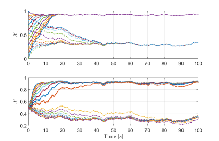
Figure 4: State trajectories of the flexibility function with different initial conditions (top panel) and different baseline (bottom panel). state trajectories affected by $u^{*}=0$ and $u^{*}=1$ are depicted by solid lines and dashed lines, respectively.

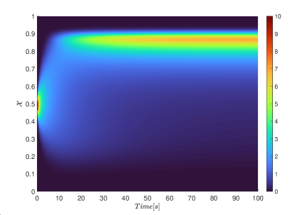
Figure 5: Probability density function (pdf) of the state of the flexibility function concerning time.

4.2 Simulation results

Energy data was carried out using the Energy Zone Model in IDA-ICE v.4.8 [35] for a neighborhood that will be built in Fredrikstad, which is a town located approximately 90 km south of Oslo, Norway. The total development consists of more than 1500 dwellings, a kindergarten, a school, and commercial buildings [36]. The data was then employed to identify the parameters of the flexibility function.

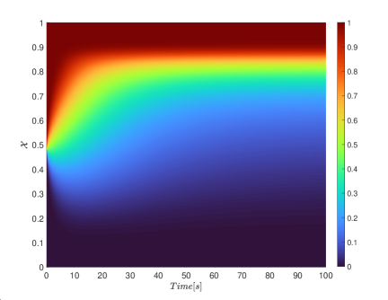
Figure 6: Comulative density function (cdf) of the state of the flexibility function with respect to time.

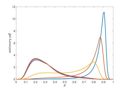
Figure 7: Stationary pdf with respect to price change.

Figure 4 demonstrates the simulation results of the stochastic flexibility function with parameters $C=2.97$, $\sigma_{X}=0.1$ and $\Delta=1$. The top panel of this figure shows the state trajectories with different initial conditions, $\mathcal{X}_{t_{0}}$, and price inputs, $u^{*}$. The second panel illustrates the state trajectories with different baseline signals, $B^{*}$, and price inputs, $u^{*}$. The state trajectories move toward different equilibrium points, $X^{*}=1$ and $X^{*}=0$, respectively, and remain in a neighborhood of them. These results follow the stability and boundedness results of Theorems 4.1 and 4.1.

The probability density function of the state of the flexibility function concerning time is shown in Figure 5. It is seen that with the initial state of $0.5$ and and constant price of $0.2$, the state will converge to a value around $0.86$ with high probability. Figure 6 shows the cumulative distribution function (cdf) of the state with respect to time. At the initial time, $P(\mathcal{X}<0.5)$ is very small. However, as time passes, $P(\mathcal{X}<0.85)$ becomes small. This result is along with the results of pdf in Figure 5.

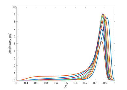
Figure 8: Stationary pdf for baseline change.

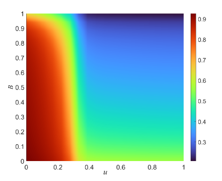
Figure 9: Mean of the stationary values of state with respect to different values of $u$ and $B$.

Stationary pdf results are provided in Figures 7 and 8. In Figure 7, a stationary pdf is demonstrated concerning various price values. It is seen that for some price values, the state converges to a neighborhood of one, and for others, it converges to a neighborhood of zero. Figure 8 shows that the trajectories converge to a large value (more energy saving), with high probability, once the price is low, i.e. $0.2$, regardless of changing the baseline.

Figure 9 illustrates the stationary mean values with respect to different values of $u$ and $B$. As expected, low energy price increases the tendency to store more energy and therefore, lead to higher stored energy. Also, at high prices, a high baseline leads to the lowest energy storage. The storage is slightly more when the baseline is low. The variance of the stationary values of the state corresponding to different values of $u$ and $B$ are shown in Figure 10. It is seen that low price leads to a tendency for higher energy storage. The variance is higher for higher energy prices and the highest when the baseline is high while the price is low. Maximum of the absolute value of nonzero eigenvalue of the generator of the Markov chain [27] with respect to various values of $u$ and $B$ are demonstrated in Figure 11. It is seen that when the price is low, it starts saving energy in a short period of time. When the baseline is high, the energy storage takes place for a longer period of time. Moreover, higher prices lead to some sort of reluctance to change the energy storage in the system.

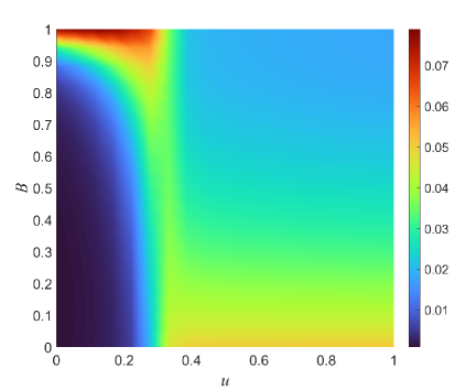
Figure 10: Variance of the stationary values of state with respect to various values of $u$ and $B$.

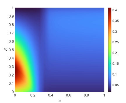
Figure 11: Maximum nonzero eigenvalue of the generator of the Markov chain with respect to various values of $u$ and $B$.

5 Conclusions

In this paper, we analyzed the stability of the flexibility functions, which is an established model of the nonlinear, dynamic, price-demand relationship in energy systems. The stability of the deterministic flexibility function, as a simplified version of the flexibility function, was first investigated. Then, the general stochastic flexibility function is considered and its stability and boundedness are analyzed. Simulation results follow the analysis and illustrate the function’s stability properties.

This work is supported by Sustainable plus energy neighbourhoods (syn.ikia) (H2020 No. 869918), ELEXIA (Horizon Europe No. 101075656), IEA EBC - Annex 81 - Data-Driven Smart Buildings (EUDP Project No. 64019-0539), IEA EBC - Annex 82 - Energy Flexible Buildings Towards Resilient Low Carbon Energy Systems (EUDP Project No. 64020-2131), and the projects DynFlex and PtX, Sector Coupling and LCA, which both are part of the Danish Mission Green Fuel portfolio of projects.

References

- [1] World Meteorological Organization (WMO). State of the climate in europe 2022. WMO: World Meteorological Organisation, 2023.
- [2] Bing Zhu, Xiaohua Xia, and Zhou Wu. Evolutionary game theoretic demand-side management and control for a class of networked smart grid. Automatica, 70:94–100, 2016.
- [3] Xuan Zhang and Antonis Papachristodoulou. A real-time control framework for smart power networks: Design methodology and stability. Automatica, 58:43–50, 2015.
- [4] Yanfang Mo, Wei Chen, Li Qiu, and Pravin Varaiya. Market implementation of multiple-arrival multiple-deadline differentiated energy services. Automatica, 116:108933, 2020.
- [5] Fabiano Pallonetto, Mattia De Rosa, Francesco D’Ettorre, and Donal P Finn. On the assessment and control optimisation of demand response programs in residential buildings. Renewable and Sustainable Energy Reviews, 127:109861, 2020.
- [6] Maryam H Shoreh, Pierluigi Siano, Miadreza Shafie-khah, Vincenzo Loia, and João PS Catalão. A survey of industrial applications of demand response. Electric Power Systems Research, 141:31–49, 2016.
- [7] Vladimir Z Gjorgievski, Natasa Markovska, Alajdin Abazi, and Neven Duić. The potential of power-to-heat demand response to improve the flexibility of the energy system: An empirical review. Renewable and Sustainable Energy Reviews, 138:110489, 2021.
- [8] A Rezaee Jordehi. Optimisation of demand response in electric power systems, a review. Renewable and sustainable energy reviews, 103:308–319, 2019.
- [9] Meisam Farrokhifar, Hamidreza Bahmani, Behdad Faridpak, Amin Safari, David Pozo, and Marco Aiello. Model predictive control for demand side management in buildings: A survey. Sustainable Cities and Society, 75:103381, 2021.
- [10] José R Vázquez-Canteli and Zoltán Nagy. Reinforcement learning for demand response: A review of algorithms and modeling techniques. Applied energy, 235:1072–1089, 2019.
- [11] Thibault Q Péan, Jaume Salom, and Ramon Costa-Castelló. Review of control strategies for improving the energy flexibility provided by heat pump systems in buildings. Journal of Process Control, 74:35–49, 2019.
- [12] Evangelos Vrettos, Emre C Kara, Jason MacDonald, Göran Andersson, and Duncan S Callaway. Experimental demonstration of frequency regulation by commercial buildings—part i: Modeling and hierarchical control design. IEEE Transactions on Smart Grid, 9(4):3213–3223, 2016.
- [13] Austin Coffman, Ana Bušić, and Prabir Barooah. A unified framework for coordination of thermostatically controlled loads. Automatica, 152:111002, 2023.
- [14] Daniela Yassuda Yamashita, Ionel Vechiu, and Jean-Paul Gaubert. A review of hierarchical control for building microgrids. Renewable and Sustainable Energy Reviews, 118:109523, 2020.
- [15] Giulia De Zotti, S Ali Pourmousavi, Henrik Madsen, and Niels Kjølstad Poulsen. Ancillary services 4.0: A top-to-bottom control-based approach for solving ancillary services problems in smart grids. Ieee Access, 6:11694–11706, 2018.
- [16] Giulia De Zotti, S Ali Pourmousavi, Juan M Morales, Henrik Madsen, and Niels Kjølstad Poulsen. A control-based method to meet tso and dso ancillary services needs by flexible end-users. IEEE Transactions on Power Systems, 35(3):1868–1880, 2019.
- [17] Georgios Tsaousoglou, Juan S Giraldo, and Nikolaos G Paterakis. Market mechanisms for local electricity markets: A review of models, solution concepts and algorithmic techniques. Renewable and Sustainable Energy Reviews, 156:111890, 2022.
- [18] Vipin Chandra Pandey, Nikhil Gupta, Khaleequr Rehman Niazi, Anil Swarnkar, and Rayees Ahmad Thokar. A hierarchical price-based demand response framework in distribution network. IEEE Transactions on Smart Grid, 13(2):1151–1164, 2021.
- [19] Georgios Tsaousoglou, Polyzois Soumplis, Nikolaos Efthymiopoulos, Konstantinos Steriotis, Aristotelis Kretsis, Prodromos Makris, Panagiotis Kokkinos, and Emmanouel Varvarigos. Demand response as a service: Clearing multiple distribution-level markets. IEEE Transactions on Cloud Computing, 10(1):82–96, 2021.
- [20] He Hao, Charles D Corbin, Karanjit Kalsi, and Robert G Pratt. Transactive control of commercial buildings for demand response. IEEE Transactions on Power Systems, 32(1):774–783, 2016.
- [21] Seyed Shahabaldin Tohidi, Davide Cali, Meril Tamm, Joana Ortiz, Jaume Salom, and Henrik Madsen. From white-box to grey-box modelling of the heat dynamics of buildings. In E3S Web of Conferences, volume 362, page 12002. EDP Sciences, 2022.
- [22] Rune Grønborg Junker, Armin Ghasem Azar, Rui Amaral Lopes, Karen Byskov Lindberg, Glenn Reynders, Rishi Relan, and Henrik Madsen. Characterizing the energy flexibility of buildings and districts. Applied energy, 225:175–182, 2018.
- [23] Rune Grønborg Junker, Carsten Skovmose Kallesøe, Jaume Palmer Real, Bianca Howard, Rui Amaral Lopes, and Henrik Madsen. Stochastic nonlinear modelling and application of price-based energy flexibility. Applied Energy, 275:115096, 2020.
- [24] Dominik Franjo Dominković, Rune Grønborg Junker, Karen Byskov Lindberg, and Henrik Madsen. Implementing flexibility into energy planning models: Soft-linking of a high-level energy planning model and a short-term operational model. Applied Energy, 260:114292, 2020.
- [25] Christian Ankerstjerne Thilker, Rune Grønborg Junker, Peder Bacher, John Bagterp Jørgensen, and Henrik Madsen. Model predictive control based on stochastic grey-box models. In Towards Energy Smart Homes: Algorithms, Technologies, and Applications, pages 329–380. Springer, 2012.
- [26] Tjerk Stegink, Claudio De Persis, and Arjan van der Schaft. A unifying energy-based approach to stability of power grids with market dynamics. IEEE Transactions on Automatic Control, 62(6):2612–2622, 2016.
- [27] Uffe Høgsbro Thygesen. Stochastic Differential Equations for Science and Engineering. CRC Press, 2023.
- [28] James O Ramsay. Monotone regression splines in action. Statistical science, pages 425–441, 1988.
- [29] Amos Schledorn, Sandrine Charousset-Brignol, Rune Grønborg Junker, Daniela Guericke, Henrik Madsen, and Dominik Franjo Dominković. Frigg 2.0: Integrating price-based demand response into large-scale energy system analysis. Applied Energy, 364:122960, 2024.
- [30] Hassan K Khalil. Nonlinear systems. Patience Hall, 2002.
- [31] Héctor J Sussmann. On the gap between deterministic and stochastic ordinary differential equations. The Annals of Probability, pages 19–41, 1978.
- [32] Harold Joseph Kushner and Kushner. Stochastic stability and control, volume 33. Academic press New York, 1967.
- [33] Uffe Høgsbro Thygesen et al. A survey of lyapunov techniques for stochastic differential equations. Citeseer, 1997.
- [34] Thomas C. Gard. Introduction to Stochastic Differential Equations. Dekker, 1988.
- [35] EQUA Simulation AB. Ida indoor climate and energy. https://www.equa.se/en/ida-ice [Accessed: (October 2022)].
- [36] Seyed Shahabaldin Tohidi, Davide Cali, Niki Gaitani, Hannes Harter, Tonje Healey Trulsrud, Jaume Salom, Francesc Madrid Lozano, Meril Tamm, Linda Hoes, Ruud van der Linden, Wouter Borsboom, and Magyari Ábel. Syn.ikia project: D4.2 characterization of the thermodynamic properties of the demonstration cases, 2022.