ksblue \addauthorkcmagenta \addauthorvsred \addauthorvsblue \addauthorhlred \addauthorvspurple \addauthorkfblue
Direct Preference Optimization With Unobserved Preference Heterogeneity
Abstract
RLHF has emerged as a pivotal step in aligning language models with human objectives and values. It typically involves learning a reward model from human preference data and then using reinforcement learning to update the generative model accordingly. Conversely, Direct Preference Optimization (DPO) directly optimizes the generative model with preference data, skipping reinforcement learning. However, both RLHF and DPO assume uniform preferences, overlooking the reality of diverse human annotators. This paper presents a new method to align generative models with varied human preferences. We propose an Expectation-Maximization adaptation to DPO, generating a mixture of models based on latent preference types of the annotators. We then introduce a min-max regret ensemble learning model to produce a single generative method to minimize worst-case regret among annotator subgroups with similar latent factors. Our algorithms leverage the simplicity of DPO while accommodating diverse preferences. Experimental results validate the effectiveness of our approach in producing equitable generative policies.
1 Introduction
Reinforcement Learning from Human Feedback (RLHF) has emerged as one of the leading methods to align Language Models (LMs) to human preferences [27, 36, 39]. RLHF focuses on learning a single reward model from human preference data and uses that to fine-tune and align the LM. To sidestep potentially expensive reinforcement learning, Direct Preference Optimization (DPO) [29] is an alignment method that optimizes the LM policy directly using the preference data. However, DPO implicitly uses the same reward model as RLHF to train the LM. This reward model reflects the majority opinion of the preference data annotators and caters to that majority. If the annotator population is not representative of the general population, then this comes at the cost of neglecting groups underrepresented in the annotators, leading to misrepresentation of preferences. On the other hand, if the annotator population is representative, then opinions of minority groups in the general population are shunned, causing bias and discrimination.
Most papers that try to deal with this issue learn a reward model and then use a standard RL framework such as PPO to align the LM. However, DPO has several advantages over RLHF, eliminating the need for a reward model and leading to a more stable pipeline. [45] utilizes these benefits by developing an algorithm that directly optimizes policy by implicitly learning a multi-objective reward model. However, methods that rely on a multi-dimensional reward model [38, 45] implicitly or explicitly have two main drawbacks. First, these methods typically require annotators to rate data on a multi-dimensional scale, with each dimension corresponding to a different objective like safety or accuracy. This data is both more costly and harder to obtain compared to binary preference data [9]. Second, the different rating objectives must be determined ahead of the data collection stage. This can be a difficult task as there are many latent factors factors that might affect the preferences of annotators [34], which can be difficult to discern. For example, if we collect ratings based on helpfulness and harmfulness similar to [4], these rankings might not fully explain some preference decisions made because of cultural, political, or geographical inclinations.
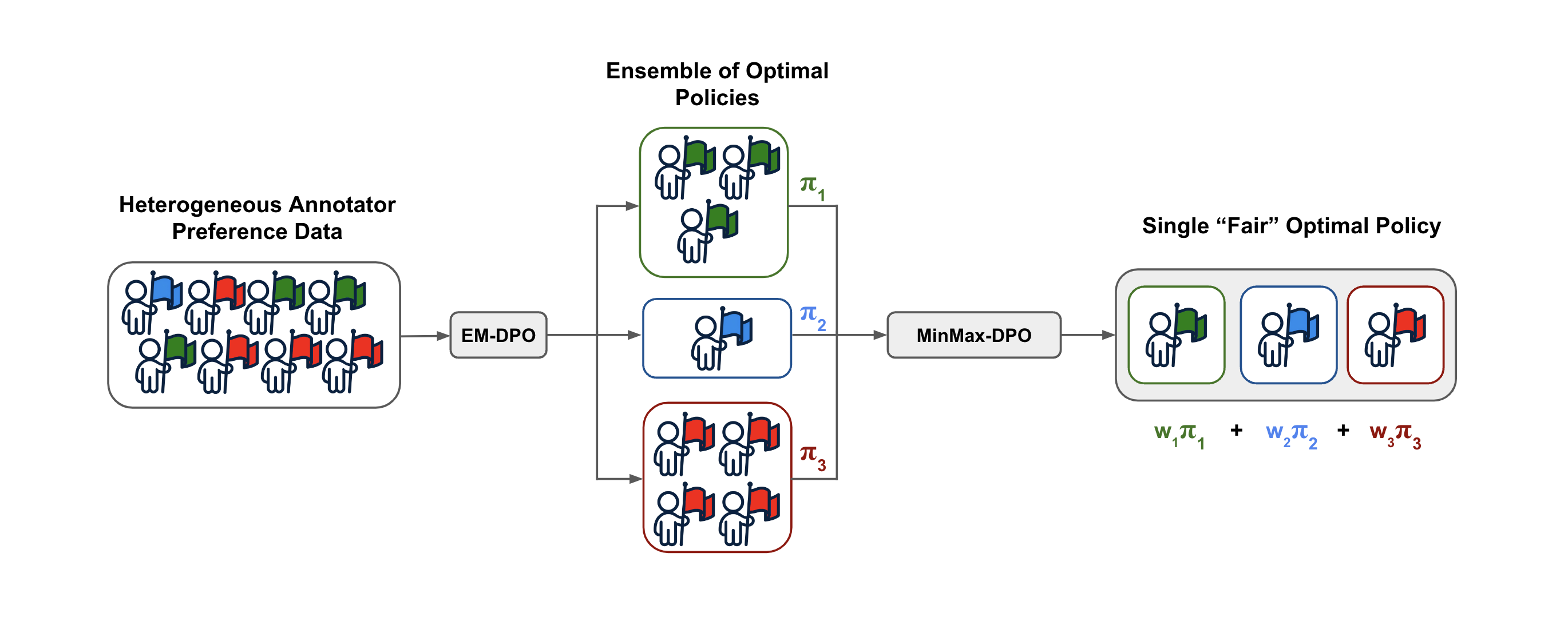
We propose two algorithms to sidestep the need for RLHF in a heterogeneous population, allowing us to cater to diverse preferences without the need for reinforcement learning, letting us reap the added benefits of DPO. In particular, we propose Expectation Maximization Direct Preference Optimization (EM-DPO) and MinMax Direct Preference Optimization (MinMax-DPO). EM-DPO uses an EM algorithm [13] to simultaneously learn the distribution of user preference types as well as policies for each type. Note that, if we already knew the group each user belonged to, we could simply train an optimal policy on each group separately. Since we do not, we think of our data as being generated by latent mixture model, where for each user we first draw a latent preference type and then draw a set of annotation data based on the preference type. We show that one can combine ideas from DPO with the EM algorithm for learning mixture models and directly learn a distribution of latent types, as well as a regularized optimal policy for each type. MinMax-DPO then takes these optimal policies and learns one model to best serve the needs of the population. Figure 1 shows the proposed pipeline.
2 Related Literature
Preference-Based Reinforcement Learning: Reinforcement learning from preferences has been an active research area for some time, providing a way to train on tasks for which explicitly defining rewards is hard [40, 21, 1]. In particular, [11, 19] show that using human preferences to guide reinforcement learning (RLHF) is particularly effective on a variety of tasks, such as training robots. More recently, RLHF has become a very popular technique to fine-tune language models to do a variety of tasks such as summarization [27, 46, 36, 41]. RLHF has also been used to align language models [4, 2]. [9] details several open problems in the field of RLHF, including those related to the feedback itself, particularly the inverse relation between richness and efficiency. Some work has been done on this problem with regards to language-based feedback in particular [16, 44] as well as in more general settings [18], but specific applications to LLMs have not been fully explored.
Challenges with Reward Modeling: In general, human preferences can be difficult to represent using reward models [17], and the validity of reward modeling itself is still somewhat debated [7, 6, 35]. Some work has also been done to take personality into account when reward modeling [23, 21], but this area remains open. In general, taking human irrationality into account when reward modeling (to optimize a more accurate reward function) leads to a trade-off between efficiency and accuracy [33, 26]. Work has been done on inverse RL with particular models of suboptimality such as myopia [15], noise [42], and risk-sensitivity [24], but dealing with general irrationalities remains open.
RLHF With Diverse Preferences: One of the chief issues in RLHF is that of diverse populations; different annotators could have very different preferences. Several studies have tried to solve the diverse population problem by learning more expressive reward functions and then using them to perform RLHF. For example, [31, 20, 10] maintains and learns several reward models at once. Similarly, [38, 45] learn a multi-dimensional reward model where each dimension provides rewards based on a different objective such as safety or usefulness. Alternatively, [34, 22] learns a distribution over fixed reward models. Finally, these reward models are combined using various strategies [5, 20, 31] to get a final reward model which is then used to perform RLHF. [10] also learns multiple reward models, but performs RL by maximizing the minimum reward thereby ensuring that the final model is fair. The paper draws on elements of social choice theory, which [12] argues is an effective path forward for RLHF research in general, specifically regarding issues with aggregating preferences. In an orthogonal approach, [43] utilizes meta-learning to learn diverse preferences. In general, trying to do RLHF with many reward models becomes expensive, making extending DPO [29] an attractive alternative. [37] proposes SPO to sidestep reinforcement learning using the concept of a minimax winner from social choice theory, but only in the case of homogeneous preferences. In concurrent work, [28] proposes a personalized RLHF algorithm which learns clustered policies via a hard Expectation Maximization algorithm using DPO. We instead propose a soft-clustering algorithm, which enjoys stronger theoretical guarantees [13]. [28] also proposes an algorithm to aggregate estimated reward functions for a heterogeneous population. We instead propose a complete pipeline to learn one equitable policy for a heterogeneous population without appealing to reward model estimation at all.
3 Background
In this section, we discuss traditional alignment methods that assume uniform preference among the whole population, namely RLHF [46, 36, 27] and DPO [29].
Reinforcement Learning from Human Feedback (RLHF) The RLHF pipeline has two inputs. The first is an LM that is pre-trained on internet-scale data and then fine-tuned with supervised learning. The second input is a static annotator preference dataset. To collect this data, first pairs of responses are generated from where is a given prompt. Human annotators then choose the best response between the two - in what follows, let denote the winning response and denote the losing response. Also, let be the population of all human annotators and be the random variable that represents a single human annotator.
In the first step of RLHF, a reward model is fit using the preference data. This is done by minimizing the following log-likelihood loss:
| (1) |
To simplify this objective, assume that the relation between preference data and rewards follows the Bradley-Terry-Luce model [8]. Let represent the true rewards for all annotators. Then, according to the BTL model, the probability that an annotator prefers one response over the other is given by:
| (2) |
so the log-likelihood loss to minimize is equivalent to
| (3) |
The second and final step is fine-tuning with reinforcement learning (RL) using the learned reward model . More specifically, the Proximal Policy Optimization (PPO) [32] is used in training the LM. The PPO algorithm optimizes the following objective:
| (4) |
Direct Preference Optimization (DPO) DPO optimizes the same objective as PPO as given in Equation 4 but bypasses learning the reward model by directly optimizing with the preference data by combining Equation 2 and Equation 4. This results in a pipeline that is not only significantly simpler, but also exhibits greater stability [29].
DPO minimizes the following log-likelihood loss directly using preference data to obtain :
| (5) |
Both RLHF and DPO assume that preferences are uniform across the population and implicitly or explicitly learn a single reward model. However, this is not the case in the real world as humans have diverse preferences and values. Moreover, RLHF and DPO prioritize the majority opinion of the annotator population. This could lead to misalignment if the annotation population is not representative of the general population. Traditional methods like RLHF and DPO can therefore lead to bias and discrimination towards the minority subgroups among the annotator population. We propose a new algorithm, MinMax-DPO, that learns an equitable and fair optimal policy directly from binary preference data to bridge this gap.
4 EM-DPO: Probabilistic Direct Preference Optimization Algorithm
The Expectation-Maximization Algorithm [13, 25] deals with settings with mixture data. Data are produced by first drawing a set of latent factors and then drawing a set of observed variables . The parameters of the likelihood determine both the distribution of the latent factors as well as the conditional likelihood . At step of the algorithm, we have a current candidate parameter vector and calculate as follows:
| (6) |
In our setting, the latent factors correspond to the unobserved heterogeneity types of an annotator and correspond to the chosen preferences for each of the prompts assigned to the annotator. We assume for simplicity that each annotator is assigned prompts and we let , where is the prompt and is the preference for that prompt. Our parameters are , where are the parameters for the group-wise policies, the latent distribution of user types and are parameters that determine the distribution of prompts .
With some calculation, we find that a parameterization of the policy implies a parameterization of the likelihood (see Appendix A):
| (7) |
where the function is similar to the parameterization introduced in DPO:
| (8) |
Note that the latent factors take values in a set of discrete values . In this case, we can assume a fully non-parametric likelihood , where , the -dimensional simplex. Subsequently, we can decompose the criterion as:
| (9) |
For further simplification, we note that to get that
| (10) |
Assuming that does not depend on the vector , so that , the original criterion decomposes into two separate optimization problems:
| (11) | ||||
For the -step, we must characterize the posterior distribution of the latent factors. Under the assumption that the contexts are un-correlated with the unobserved preference types, which is natural in the context of LLM fine-tuning, since contexts are randomly assigned to annotators, we can derive that (see Appendiex B):
| (12) |
For the -step, we must solve the two optimization problems given above. The solution for can be derived in closed form, while the solution for is independent of the term :
| (13) | ||||
| (14) |
A full derivation is in Appendix C. This gives rise to the following EM algorithm:
Note that if we do not share parameters across the policies for each preference type , i.e. we have separate parameters for each , then the optimization in the final step of EM-DPO also decomposes into separate policy optimization problems for each preference type:
| (15) |
Note that the latter is simply a weighted DPO problem, where each demonstration , which corresponds to the -th demonstrations from annotator , is assigned weight when optimizing the policy parameters for preference type . Alternatively, for multi-tasking purposes, some parameters can be shared parameters across policies for each preference type, in which case the final optimization problem should be solved simultaneously via stochastic gradient descent over the joint parameters .
5 MinMax-DPO: Direct Optimization for Min-Max Regret Ensemble
5.1 MinMax Regret Objective
So far, we have shown how to calculate a separate policy that optimizes for each preference population . Our ultimate goal is to output a single policy. Hence, we need to trade-off optimizing for the preferences of different groups and find a policy that strikes a good balance.
In that respect, to equitably cater to all sub-populations, we focus on identifying a policy that minimizes the worst-case regret among the sub-populations. To avoid having to retrain a new policy, we will restrict ourselves to selecting an ensemble among the already trained policies. As such, we define the ensemble space of policies as:
| (16) |
If we had access to the reward functions , then for any policy , the expected reward that population receives would be:
| (17) |
Note that if we were to solely focus on population , we would be optimizing the expected reward objective above, regularized so as not to deviate from the reference policy. This would yield policy , where are the policy parameters we calculated based on the EM-DPO algorithm.
Our goal is to find an ensemble policy such that no population has very large regret towards choosing their population-preferred policy . Our minimax regret optimization problem can be simply stated as:
| (18) |
where . Note that we only consider the positive part of the regret.
Why min-max regret? Max-min reward is another fairness criterion that can be applied to the RLHF problem to ensure equity, as discussed in [10]. However, this criterion has two major drawbacks. Firstly, the reward model is not uniquely identifiable from preference data. Two reward models and are equivalent if [29]. Therefore, directly maximizing the minimum reward is ineffective due to this scaling. We could fix this by standardizing the reward model to set the minimum reward to zero - if is the recovered reward function, we can use , which is an equivalent reward model. Even then, there is another issue with the max-min reward criterion.
The max-min reward focuses on improving rewards for users with the lowest reward, while the min-max regret function targets users with the highest regrets. These groups differ when users with low rewards also have low regrets. As an example, consider a setting with fixed context and three responses. If two users have reward vectors [0, 0.01, 0.02] and [0, 10, 1] respectively, then the max-min reward objective will choose response 3 to maximize user 2’s reward. However, user 1 is nearly indifferent between the three choices 2, whereas user 2 strongly prefers option 2. Therefore, it is more ideal to choose option 2, which the min-max regret criteria chooses.
5.2 Regret Dynamics
We now show that the min-max regret objective can also be optimized over, without access to the explicit reward functions, but solely based on the policies we have already trained. We can rewrite our objective as (see Appendix D):
| (19) |
where
| (20) |
Letting denote the matrix whose entry (for ) corresponds to we can re-write the above objective as:
| (21) |
This is simply a finite action zero-sum game, where the minimizing player has actions and the maximizing player has actions. A large variety of methods can be utilized to calculate an equilibrium of this zero-sum game and hence identify the minimax regret optimal mixture weights . For instance, we can employ optimistic Hedge vs. optimistic Hedge dynamics, which are known to achieve fast convergence rates in such finite action zero-sum games [30] and then use the average of the solutions over the iterates of training, as described in Algorithm 2.
The solution returned by Algorithm 2 consistutes a -approximate solution to the min-max regret problem (a direct consequence of the results in [30]). This completes our overall direct preference optimization procedure with unobserved heterogeneous preferences.
One can also optimize a new policy that does not correspond to an ensemble of the base policies by solving the saddle point problem:
| (22) |
which has already been shown, can be expressed as a function of and . This saddle point can be solved by policy-gradient vs multiplicative weight dynamics, or for faster convergence via optimistic policy gradient descent vs optimistic mulitplicative weight dynamics:
| (23) | ||||
| (24) |
6 Experiments
6.1 Experiment Setting
We can draw parallels between the offline contextual bandit problem and the problem of learning from human preferences [3]. In this setting, the context represents the prompt and the bandit arms represent the possible responses for the given context. For our experiment, we consider a simplified case with three arms.
First, we generate 200 annotators drawn randomly from three sub-populations, with 60% of the population coming from the first sub-population, 30% from the second, and 10% from the third. The preferences of annotators within each sub-population is homogeneous and therefore, each sub-population is associated with a single reward model. For our experiment, we model the sub-population reward model using a linear function, similarly to linear contextual bandits [14]:
| (25) |
where is the model parameters corresponding to the latent variable for arm , is the context, and represents noise with mean and standard deviation . is fixed for any given sub-population with values and for sub-population . We generate 10 preference data pairs per annotator. For each data point, first we draw a context vector uniformly randomly from the hypercube . Then, a pair of responses is generated from a uniformly random reference policy . The annotator then chooses a response based on their reward model . We implement EM-DPO and MinMax-DPO for this data. Appendix E shows hyperparameters for the experiment.
6.2 Results
We run standard DPO and MinMax-DPO on this experimental setup and calculate the average regret per user group. The results of this are shown in Figure 2.
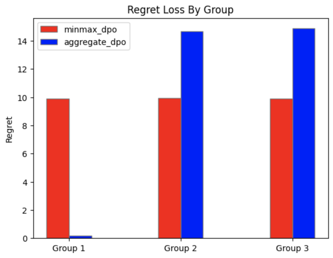
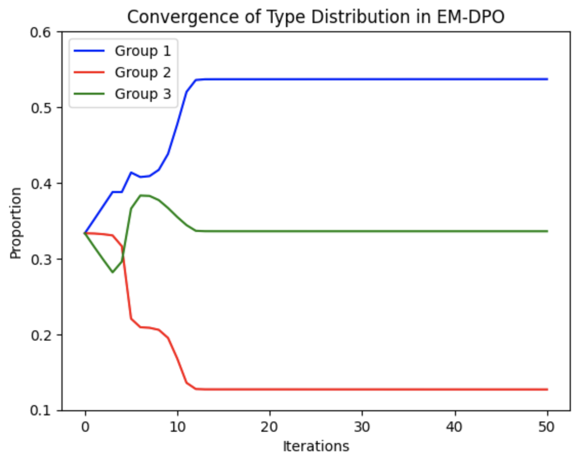
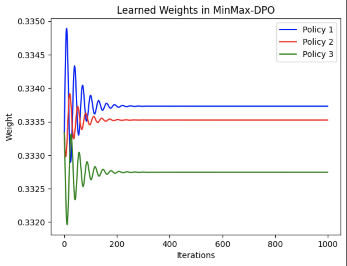
We can see that training DPO over the whole population leads to the policy completely optimizing for the first user group’s preference (i.e., majority opinion), leading to maximal regret for the other two groups. However, MinMax-DPO achieves the social optimum and respects the preferences of all three groups, as shown by the equal regret among all three groups. Figure 3 shows the convergence of (learning the latent distribution of users) during EM-DPO. The true distribution of users for the given seed was 53.5%, 33.5%, and 13% and the algorithm exactly converges to that distribution. Figure 4 shows the convergence of the learned weights in the MinMax-DPO algorithm; we see relatively quick convergence to the optimal weights, which are close to uniform. This is expected as all three sub-groups have perfectly contradicting opinions because they each prefer a different response.
6.3 Discussion & Limitations
We provide a robust framework to train equitable policies for a heterogeneous population with diverse preferences. By extending the DPO algorithm, we are able to sidestep reinforcement learning entirely, enjoying the added stability that DPO provides while making it more applicable to real-world situations and datasets. We demonstrate our findings on a contextual bandit experiment, showing how our algorithm, MinMax-DPO, generates a far more socially equitable policy than standard DPO in diverse populations where some groups may be underrepresented.
Based on our results, we raise some limitations and directions for future work. Our derivations operate off of the assumption that contexts are uncorrelated given the preference type of the annotator; this may not be the case in the real world as, to increase accuracy of data collection, annotators may be given prompts more tuned to their skill sets. We also assume annotators report their preferences honestly, which may not be the case - this raises important questions regarding incentive compatibility. Furthermore, it remains to be seen how MinMax-DPO and its performance over standard DPO scales to larger experiments, such as those with LLMs. Based on the bandit experiment, we expect computational efficiency to be a relative non-issue at scale.
References
- [1] Youssef Abdelkareem, Shady Shehata, and Fakhri Karray. Advances in preference-based reinforcement learning: A review. In 2022 IEEE International Conference on Systems, Man, and Cybernetics (SMC), pages 2527–2532. IEEE, 2022.
- [2] Amanda Askell, Yuntao Bai, Anna Chen, Dawn Drain, Deep Ganguli, Tom Henighan, Andy Jones, Nicholas Joseph, Ben Mann, Nova DasSarma, et al. A general language assistant as a laboratory for alignment. arXiv preprint arXiv:2112.00861, 2021.
- [3] Mohammad Gheshlaghi Azar, Zhaohan Daniel Guo, Bilal Piot, Remi Munos, Mark Rowland, Michal Valko, and Daniele Calandriello. A general theoretical paradigm to understand learning from human preferences. In International Conference on Artificial Intelligence and Statistics, pages 4447–4455. PMLR, 2024.
- [4] Yuntao Bai, Andy Jones, Kamal Ndousse, Amanda Askell, Anna Chen, Nova DasSarma, Dawn Drain, Stanislav Fort, Deep Ganguli, Tom Henighan, et al. Training a helpful and harmless assistant with reinforcement learning from human feedback. arXiv preprint arXiv:2204.05862, 2022.
- [5] Michiel Bakker, Martin Chadwick, Hannah Sheahan, Michael Tessler, Lucy Campbell-Gillingham, Jan Balaguer, Nat McAleese, Amelia Glaese, John Aslanides, Matt Botvinick, et al. Fine-tuning language models to find agreement among humans with diverse preferences. Advances in Neural Information Processing Systems, 35:38176–38189, 2022.
- [6] Andreea Bobu, Andi Peng, Pulkit Agrawal, Julie Shah, and Anca D Dragan. Aligning robot and human representations. arXiv preprint arXiv:2302.01928, 2023.
- [7] Michael Bowling, John D Martin, David Abel, and Will Dabney. Settling the reward hypothesis. In International Conference on Machine Learning, pages 3003–3020. PMLR, 2023.
- [8] Ralph Allan Bradley and Milton E Terry. Rank analysis of incomplete block designs: I. the method of paired comparisons. Biometrika, 39(3/4):324–345, 1952.
- [9] Stephen Casper, Xander Davies, Claudia Shi, Thomas Krendl Gilbert, Jérémy Scheurer, Javier Rando, Rachel Freedman, Tomasz Korbak, David Lindner, Pedro Freire, et al. Open problems and fundamental limitations of reinforcement learning from human feedback. arXiv preprint arXiv:2307.15217, 2023.
- [10] Souradip Chakraborty, Jiahao Qiu, Hui Yuan, Alec Koppel, Furong Huang, Dinesh Manocha, Amrit Singh Bedi, and Mengdi Wang. Maxmin-rlhf: Towards equitable alignment of large language models with diverse human preferences. arXiv preprint arXiv:2402.08925, 2024.
- [11] Paul F Christiano, Jan Leike, Tom Brown, Miljan Martic, Shane Legg, and Dario Amodei. Deep reinforcement learning from human preferences. Advances in neural information processing systems, 30, 2017.
- [12] Vincent Conitzer, Rachel Freedman, Jobst Heitzig, Wesley H Holliday, Bob M Jacobs, Nathan Lambert, Milan Mossé, Eric Pacuit, Stuart Russell, Hailey Schoelkopf, et al. Social choice for ai alignment: Dealing with diverse human feedback. arXiv preprint arXiv:2404.10271, 2024.
- [13] Arthur P Dempster, Nan M Laird, and Donald B Rubin. Maximum likelihood from incomplete data via the em algorithm. Journal of the royal statistical society: series B (methodological), 39(1):1–22, 1977.
- [14] Maria Dimakopoulou, Zhengyuan Zhou, Susan Athey, and Guido Imbens. Balanced linear contextual bandits. In Proceedings of the AAAI Conference on Artificial Intelligence, volume 33, pages 3445–3453, 2019.
- [15] Owain Evans, Andreas Stuhlmüller, and Noah Goodman. Learning the preferences of ignorant, inconsistent agents. In Proceedings of the AAAI Conference on Artificial Intelligence, volume 30, 2016.
- [16] Justin Fu, Anoop Korattikara, Sergey Levine, and Sergio Guadarrama. From language to goals: Inverse reinforcement learning for vision-based instruction following. arXiv preprint arXiv:1902.07742, 2019.
- [17] Joey Hong, Kush Bhatia, and Anca Dragan. On the sensitivity of reward inference to misspecified human models. arXiv preprint arXiv:2212.04717, 2022.
- [18] Minyoung Hwang, Gunmin Lee, Hogun Kee, Chan Woo Kim, Kyungjae Lee, and Songhwai Oh. Sequential preference ranking for efficient reinforcement learning from human feedback. Advances in Neural Information Processing Systems, 36, 2024.
- [19] Borja Ibarz, Jan Leike, Tobias Pohlen, Geoffrey Irving, Shane Legg, and Dario Amodei. Reward learning from human preferences and demonstrations in atari. Advances in neural information processing systems, 31, 2018.
- [20] Joel Jang, Seungone Kim, Bill Yuchen Lin, Yizhong Wang, Jack Hessel, Luke Zettlemoyer, Hannaneh Hajishirzi, Yejin Choi, and Prithviraj Ammanabrolu. Personalized soups: Personalized large language model alignment via post-hoc parameter merging. arXiv preprint arXiv:2310.11564, 2023.
- [21] Kimin Lee, Laura Smith, Anca Dragan, and Pieter Abbeel. B-pref: Benchmarking preference-based reinforcement learning. arXiv preprint arXiv:2111.03026, 2021.
- [22] Dexun Li, Cong Zhang, Kuicai Dong, Derrick Goh Xin Deik, Ruiming Tang, and Yong Liu. Aligning crowd feedback via distributional preference reward modeling. arXiv preprint arXiv:2402.09764, 2024.
- [23] David Lindner and Mennatallah El-Assady. Humans are not boltzmann distributions: Challenges and opportunities for modelling human feedback and interaction in reinforcement learning. arXiv preprint arXiv:2206.13316, 2022.
- [24] Anirudha Majumdar, Sumeet Singh, Ajay Mandlekar, and Marco Pavone. Risk-sensitive inverse reinforcement learning via coherent risk models. In Robotics: science and systems, volume 16, page 117, 2017.
- [25] Todd K Moon. The expectation-maximization algorithm. IEEE Signal processing magazine, 13(6):47–60, 1996.
- [26] Khanh Nguyen, Hal Daumé III, and Jordan Boyd-Graber. Reinforcement learning for bandit neural machine translation with simulated human feedback. arXiv preprint arXiv:1707.07402, 2017.
- [27] Long Ouyang, Jeffrey Wu, Xu Jiang, Diogo Almeida, Carroll Wainwright, Pamela Mishkin, Chong Zhang, Sandhini Agarwal, Katarina Slama, Alex Ray, et al. Training language models to follow instructions with human feedback. Advances in neural information processing systems, 35:27730–27744, 2022.
- [28] Chanwoo Park, Mingyang Liu, Kaiqing Zhang, and Asuman Ozdaglar. Principled rlhf from heterogeneous feedback via personalization and preference aggregation. arXiv preprint arXiv:2405.00254, 2024.
- [29] Rafael Rafailov, Archit Sharma, Eric Mitchell, Christopher D Manning, Stefano Ermon, and Chelsea Finn. Direct preference optimization: Your language model is secretly a reward model. Advances in Neural Information Processing Systems, 36, 2024.
- [30] Sasha Rakhlin and Karthik Sridharan. Optimization, learning, and games with predictable sequences. Advances in Neural Information Processing Systems, 26, 2013.
- [31] Alexandre Rame, Guillaume Couairon, Corentin Dancette, Jean-Baptiste Gaya, Mustafa Shukor, Laure Soulier, and Matthieu Cord. Rewarded soups: towards pareto-optimal alignment by interpolating weights fine-tuned on diverse rewards. Advances in Neural Information Processing Systems, 36, 2024.
- [32] John Schulman, Filip Wolski, Prafulla Dhariwal, Alec Radford, and Oleg Klimov. Proximal policy optimization algorithms. arXiv preprint arXiv:1707.06347, 2017.
- [33] Rohin Shah, Noah Gundotra, Pieter Abbeel, and Anca Dragan. On the feasibility of learning, rather than assuming, human biases for reward inference. In International Conference on Machine Learning, pages 5670–5679. PMLR, 2019.
- [34] Anand Siththaranjan, Cassidy Laidlaw, and Dylan Hadfield-Menell. Distributional preference learning: Understanding and accounting for hidden context in rlhf. arXiv preprint arXiv:2312.08358, 2023.
- [35] Joar Max Viktor Skalse and Alessandro Abate. The reward hypothesis is false. 2022.
- [36] Nisan Stiennon, Long Ouyang, Jeffrey Wu, Daniel Ziegler, Ryan Lowe, Chelsea Voss, Alec Radford, Dario Amodei, and Paul F Christiano. Learning to summarize with human feedback. Advances in Neural Information Processing Systems, 33:3008–3021, 2020.
- [37] Gokul Swamy, Christoph Dann, Rahul Kidambi, Zhiwei Steven Wu, and Alekh Agarwal. A minimaximalist approach to reinforcement learning from human feedback. arXiv preprint arXiv:2401.04056, 2024.
- [38] Haoxiang Wang, Yong Lin, Wei Xiong, Rui Yang, Shizhe Diao, Shuang Qiu, Han Zhao, and Tong Zhang. Arithmetic control of llms for diverse user preferences: Directional preference alignment with multi-objective rewards. arXiv preprint arXiv:2402.18571, 2024.
- [39] Yufei Wang, Wanjun Zhong, Liangyou Li, Fei Mi, Xingshan Zeng, Wenyong Huang, Lifeng Shang, Xin Jiang, and Qun Liu. Aligning large language models with human: A survey. arXiv preprint arXiv:2307.12966, 2023.
- [40] Christian Wirth, Riad Akrour, Gerhard Neumann, and Johannes Fürnkranz. A survey of preference-based reinforcement learning methods. Journal of Machine Learning Research, 18(136):1–46, 2017.
- [41] Jeff Wu, Long Ouyang, Daniel M Ziegler, Nisan Stiennon, Ryan Lowe, Jan Leike, and Paul Christiano. Recursively summarizing books with human feedback. arXiv preprint arXiv:2109.10862, 2021.
- [42] Jiangchuan Zheng, Siyuan Liu, and Lionel M Ni. Robust bayesian inverse reinforcement learning with sparse behavior noise. In Proceedings of the AAAI Conference on Artificial Intelligence, volume 28, 2014.
- [43] Huiying Zhong, Zhun Deng, Weijie J Su, Zhiwei Steven Wu, and Linjun Zhang. Provable multi-party reinforcement learning with diverse human feedback. arXiv preprint arXiv:2403.05006, 2024.
- [44] Li Zhou and Kevin Small. Inverse reinforcement learning with natural language goals. In Proceedings of the AAAI Conference on Artificial Intelligence, volume 35, pages 11116–11124, 2021.
- [45] Zhanhui Zhou, Jie Liu, Chao Yang, Jing Shao, Yu Liu, Xiangyu Yue, Wanli Ouyang, and Yu Qiao. Beyond one-preference-fits-all alignment: Multi-objective direct preference optimization. arXiv preprint arXiv:2310.03708, 2023.
- [46] Daniel M Ziegler, Nisan Stiennon, Jeffrey Wu, Tom B Brown, Alec Radford, Dario Amodei, Paul Christiano, and Geoffrey Irving. Fine-tuning language models from human preferences. arXiv preprint arXiv:1909.08593, 2019.
Appendix A Likelihood Parameterization
Note that, in our situation, the latent factors and observed variables are independent across annotators and therefore, the likelihood and the prior factorizes across the annotators. Moreover, conditional on the latent factor, the are independently distributed across and for each the conditional likelihood takes a logistic form, as follows:
| (26) | ||||
| (27) | ||||
| (28) |
where denotes the true reward for the annotator, as in Section 3.
The first part can also be written in closed form in terms of the policy parameters for each preference type as designated by the same observation as in \ksedit[29]:
| (29) |
where optimizes the type specific regularized objective:
| (30) |
We will introduce the shorthand notation:
| (31) |
Thus a parameterization of the policy space , implies a parameterization of the likelihood:
| (32) |
as desired.
Appendix B -Step Derivation
Here, we derive the posterior distribution for any given parameter . We apply Bayes rule:
| (33) | ||||
| (34) |
In the context of LLMs, the quantity is the prompt and the prompts are randomly assigned to annotators, so we would expect no correlation between the preference type of the annotator and the prompt assigned to them. Thus, all prompts are equally likely given the preference type of the annotator. Hence, we make the following assumption:
ASSUMPTION 1 (Un-correlated Contexts and Latent Preference Types).
For all :
| (35) |
Based on this assumption, we can then write:
| (36) |
Note that we can write:
| (37) | ||||
| (38) |
Thus, the terms cancel from the numerator and denominator in Equation (36), leading to the simplified formula that is independent of :
| (39) |
Appendix C -Step Derivation
We aim to solve the following two optimization problems:
| (40) | ||||
The first optimization problem in Equation (40) admits a closed-form solution. Letting
| (41) |
Thus the optimization problem that determines takes the simple form . The Lagrangian of this problem is . The KKT condition is:
| (42) |
Moreover, since , we have . Thus, the above simplifies to:
| (43) |
For the second optimization problem in Equation (40), we further decompose the objective:
| (44) |
Assuming that the parameter that determines that , according to Assumption 1 is not subject to joint constraints with the parameter , we can drop the second part in the objective, when optimizing for :
| (45) |
Moreover, since does not enter in the update rules for , nor in the calculation of the posterior, we can ignore it in our EM-DPO algorithm.
Appendix D Min-Max Regret Objective Derivation
We can write, by linearity of expectation:
| (46) | ||||
| (47) | ||||
| (48) |
For any , we will let:
| (49) |
Given the policy parameters we estimated in the EM-DPO section, these quantities can be calculated as simple empirical averages over the annotated data. Moreover, note that since our policy is a mixture policy over the policies for with weights , we can write:
| (50) |
Thus, our minimax regret objective can be simply written as:
| (51) |
Introducing a fake preference population that always has regret, i.e. , we can re-write the above objective simply as:
| (52) |
Appendix E Additional Experiment Details
Table 1 shows all hyperparameters for the experiment. We ran the bandit experiment on one A100 GPU. On average, the code took approximately 1 hour to run.
| Hyperparameter | Value |
|---|---|
| Neural Network Layers | 3 |
| Neural Network Hidden Dimension | 10 |
| Learning Rate | 0.01 |
| Optimizer | Adam |
| DPO Regularization Constant Beta | 1 |
| Max Epochs for Optimization | 1000 |
| Max Steps for EM-DPO | 100 |
| Max Steps for MINMAX-DPO | 1000 |
| Seed (numpy and torch) | 123 |