Reframing Spatial Reasoning Evaluation in Language Models:
A Real-World Simulation Benchmark for Qualitative Reasoning
Abstract
Spatial reasoning plays a vital role in both human cognition and machine intelligence, prompting new research into language models’ (LMs) capabilities in this regard. However, existing benchmarks reveal shortcomings in evaluating qualitative spatial reasoning (QSR). These benchmarks typically present oversimplified scenarios or unclear natural language descriptions, hindering effective evaluation. We present a novel benchmark for assessing QSR in LMs, which is grounded in realistic 3D simulation data, offering a series of diverse room layouts with various objects and their spatial relationships. This approach provides a more detailed and context-rich narrative for spatial reasoning evaluation, diverging from traditional, toy-task-oriented scenarios. Our benchmark encompasses a broad spectrum of qualitative spatial relationships, including topological, directional, and distance relations. These are presented with different viewing points, varied granularities, and density of relation constraints to mimic real-world complexities. A key contribution is our logic-based consistency-checking tool, which enables the assessment of multiple plausible solutions, aligning with real-world scenarios where spatial relationships are often open to interpretation. Our benchmark evaluation of advanced LMs reveals their strengths and limitations in spatial reasoning. They face difficulties with multi-hop spatial reasoning and interpreting a mix of different view descriptions, pointing to areas for future improvement.
1 Introduction
In recent years, advancements in language models OpenAI (2023) Touvron et al. (2023) have significantly improved their capabilities in understanding and reasoning with textual information Li et al. (2022). However, promoting these models’ ability to process and reason about spatial relationships remains a complex challenge Bang et al. (2023) Cohn and Hernandez-Orallo (2023). Spatial reasoning, a critical component of human cognition, involves understanding and navigating the relationships between objects in space Cohn and Renz (2008) Alomari et al. (2022). Existing benchmarks like bAbI Weston et al. (2016), StepGame Shi et al. (2022), SpartQAMirzaee et al. (2021), and SpaRTUN Mirzaee and Kordjamshidi (2022) have significantly contributed to the field, yet they exhibit limitations in representing the complexity and naturalness found in real-world spatial reasoning.
In this paper, we conduct an extensive analysis of task complexity and limitations in four widely used datasets for textual spatial reasoning evaluation. bAbI and StepGame, originating from simplified, toy-like tasks, utilize grid-based environments with fixed distances and angles for spatial relations. This approach for constructing spatial reasoning data, while ensuring unique solutions, oversimplifies the tasks, failing to capture the complexity of spatial relationships in the real world. Moreover, the primary challenge in StepGame lies in constructing a chain of objects from multiple shuffled relations, overshadowing the spatial reasoning aspect. Our previous research indicates that GPT-4 excels in the spatial reasoning aspects of relation mapping and coordinate calculation needed for this task once the chain is established.
On the other hand, SpartQA and SpaRTUN, which cover a wider range of spatial relationships, do not always contain clear and fluent language descriptions. Common issues observed include complex object descriptions and disordered relational sequencing. Objects are described using a combination of color, size, and shape. This level of detail complicates the narrative, shifting the focus away from spatial reasoning and towards deciphering the object descriptions. The disordered relational sequencing hinders the understanding of the core spatial problem, adding unnecessary complexity.
In response to the limitations of current benchmarks in qualitative spatial reasoning, this paper introduces a new, more comprehensive benchmark to evaluate LMs’ abilities in this domain. Our benchmark seeks to present more naturally described stories, employing language that is easily understandable and processable by both humans and LMs. We aim to move away from overly logical expressions and toward narratives that mirror everyday communication. To achieve this goal, the scenarios for our benchmark are sourced from 3D simulation data rather than toy tasks, encompassing a variety of room layouts with diverse objects, each annotated with specific attributes. This approach allows each scenario to showcase a distinct arrangement of everyday objects. During data creation, the placement of objects, their layout, and their spatial relationships with other objects are determined. This information forms the basis for generating stories, questions, and answers for each instance.
Recognizing that spatial reasoning often yields multiple plausible solutions, we focus on assessing the consistency of LMs’ answers within the given constraints rather than seeking a single ‘correct’ answer. This approach aligns with the real-world nature of spatial reasoning, where multiple interpretations are often valid.
Finally, we evaluate some LLMs’ performance on our benchmark, to offer a more nuanced and comprehensive evaluation of LLMs’ qualitative spatial reasoning ability. According to our results, GPT-4 shows superior capability in spatial reasoning tasks across various settings. All models face challenges in reasoning about spatial relations between objects as multi-hop spatial reasoning complexity increases. However, there is a clear trend toward improved performance as the story’s constraint graph becomes more complete.
This paper presents several contributions to the field of QSR evaluation, particularly in the context of LM performance. These contributions are as follows:
-
•
Comprehensive analysis of existing benchmarks. We provide an in-depth analysis of the complexity and limitations inherent in current spatial reasoning benchmarks.
-
•
Constructing a more natural and realistic benchmark by developing scenarios derived from 3D simulation data, offering a diverse series of data, each varying in the granularity of relationships and the selection of relational constraints.
-
•
Introduction of a logic-based consistency checking tool for evaluation, which evaluates whether spatial relations predicted by LMs are feasible, given the set constraints.
-
•
Detailed evaluation of LLMs’ spatial reasoning abilities. By applying our benchmark to test various LMs, we provide a refined assessment of their capabilities in QSR.
Overall, these contributions advance LM evaluation for spatial reasoning, aligning more closely with real-world scenarios and human cognitive processes.
2 Analysis of Existing QSR in Text Datasets/Benchmarks
Representative benchmarks like bAbI, StepGame, SpartQA, and SpaRTUN focus on spatial reasoning. They involve tasks where models are required to infer new spatial relations from provided facts or check the consistency of relations.
2.1 bAbI
The bAbI benchmark Weston et al. (2016), featuring a collection of synthetic tasks, was crafted to evaluate learning algorithms in terms of their text understanding and reasoning abilities. Among its 20 tasks, Tasks 17 and 19 are specifically designed for spatial reasoning evaluation.
Task 17 tests LMs’ ability to understand and reason about relative spatial relations ‘left’, ‘right’, ‘above’, and ‘below’. The task operates within a 5x5 grid environment. In this structured setting, three entities are sequentially positioned at specific nodes. The placement of each entity is determined by its spatial relation to the adjacent nodes. The narratives distinguish three entities based on their color and shape. Each example can include up to 10 sentences - 2 describing spatial relations between two pairs of objects and 8 for generating questions about a different pair, as illustrated in Figure 2. These questions are structured in a yes/no format, with answers based on the entities’ actual positions on the grid.
Task 19 is centered around identifying paths between specified objects, utilizing the four cardinal directions: north, south, east, and west. These objects are described as various locations, such as bedrooms and bathrooms. In the ‘en-valid-10k’ version of bAbI111https://www.kaggle.com/datasets/roblexnana/the-babi-tasks-for-nlp-qa-system, each story typically includes 5 sentences related to spatial relations: 2 effectively describing the path and 3 serving as decoys, as shown in Figure 2. The task’s challenge lies in mapping out a sequential path from the start entity to the end entity. The inclusion of decoy sentences adds a layer of complexity to the task.

The bAbI tasks, designed as simplified ‘toy tasks’, have limitations in testing spatial reasoning. They restrict spatial relations to basic cardinal directions north, south, west, and east (also referred to as above, below, left, and right in task 17) with set distances and angles, lacking the complexity and ambiguity of real-world spatial scenarios. Additionally, using a single template for each relation may not adequately challenge a model’s understanding and reasoning in more nuanced, context-rich environments. Consequently, while useful for basic training, bAbI tasks may not fully test or equip models for the intricacies of real-world spatial reasoning.
2.2 StepGame
Building upon bAbI, the StepGame benchmark Shi et al. (2022) utilizes a grid-based system and introduces higher complexity in three key aspects:
-
•
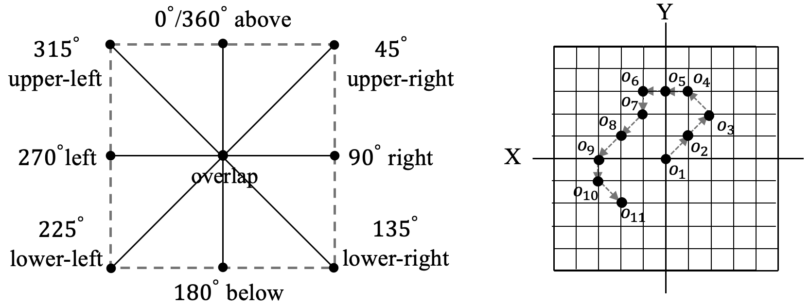
An expanded set of directional spatial relations is included, encompassing eight relations: top (north), down (south), left (west), right (east), top-left (north-west), top-right (north-east), down-left (south-west), and down-right (south-east). Each is defined by a unique angle and distance. These relations can be visually illustrated on a grid, as shown in the left diagram of Figure 3, with the inclusion of an ‘overlap’ relation for overlapping object locations.
-
•
Enhanced multi-hop reasoning challenges: Moving beyond the 4-hop reasoning in bAbI, StepGame increases the complexity to span 1-hop to 10-hop sequences. The right diagram of Figure 3 illustrates the sequential building of relational constraints, based on , the number of relationships. This produces a chain of constraints linking objects in a direct path from to , continuing through to .
-
•
Employing richer, crowdsourced narratives describing eight possible spatial relations between two entities, which serve as the basis for generating story-question pairs.
The spatial configuration used in StepGame introduces limitations that may affect the evaluation of LMs’ spatial reasoning abilities. Commonsense human understanding does not confine directional relationships to strict distance or angular constraints. For example, when we say ‘A is east of B’ in a two-dimensional framework, it simply means that the x-coordinate of A, denoted as , is larger than that of B, . This does not necessarily dictate that should exceed by an exact value or align with a specific angle, such as a 1-unit difference or a angle.
StepGame’s design yields unique solutions for all instances, but with limited complexity (as depicted in the Appendix). Prior research Li et al. (2024) indicates that the most challenging aspect for LLMs in this task is constructing the object-linking chain from shuffled relations, rather than the spatial reasoning component itself. When provided with a pre-constructed reasoning chain, GPT-4 demonstrates remarkable proficiency in handling such reasoning tasks.
2.3 SpartQA, SpaRTUN:
SpartQA Mirzaee et al. (2021) and SpaRTUN Mirzaee and Kordjamshidi (2022) start from 2D images featuring objects (rectangle, triangle, square) distributed across distinct square blocks (scenes). They extend beyond mere directional spatial relationships to include Region Connection Calculus 8 (RCC-8) Randell et al. (1992) and distance (near and far). SpaRTUN is an updated version of SpartQA-Auto and contains more relation types and rules.
Unlike the previous two grid-based benchmarks, SpartQA and SpaRTUN’s define spatial relations using a square boundary framework. Each spatial relation is determined by the coordinates of the lower-left points of the square boundary boxes of two objects and the size of these boxes.
-
•
For object-to-object relations, EC, NEAR, FAR, LEFT / RIGHT, ABOVE / BELOW are considered;
-
•
For object-to-scene relations, TPP / TPPi, and NTPP / NTPPi are considered;
-
•
For scene-to-scene relations, DC, EC, PO, TPP / TPPi, and NTPP / NTPPi are considered.
The scene description was generated from the selected story triplets using context-free grammar (CFG). They increase the variety of spatial expressions by using a vocabulary of various entity properties and relation expressions. They map the relation types and the entity properties to the lexical forms from a specifically collected vocabulary.
Although these two benchmarks include rich spatial relationships, they struggle to provide effective descriptions. They use simple syntax and word choice but lack logical flow and content clarity, particularly in two aspects:
-
•
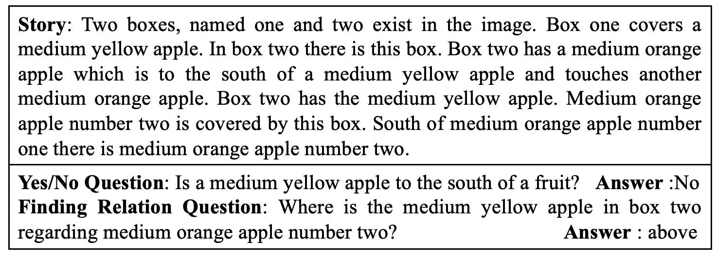
The spatial relations are described as a sequence of randomly selected story triplets, which deviates from the typical human approach to describing a scene. In the example from Figure 4, a more natural human description would typically start with outlining the relationships between two boxes, followed by detailing the contents of each box, and then explaining the relations between the objects. However, in their narrative structure, there is a lack of an initial summary of the objects contained in each box, with objects being introduced individually and somewhat disjointedly. Additionally, the narrative places the object-to-box relationships prior to the box-to-box relationships, which further diverges from the typical human method of spatial description, leading to potential confusion in understanding the overall spatial layout.
-
•
The excessive use of detailed and repetitive entity naming, involving terms like ‘medium yellow apple’, ‘medium orange apple number one’, and ‘medium orange apple number two’, results in overly lengthy text. This verbosity transforms a simple description such as ‘South of A is B’ into a more convoluted one like ‘South of medium orange apple number one is medium orange apple number two’. Such complexity not only adds confusion but also shifts the focus from understanding the spatial relationship to deciphering which specific object is being referred to. This can make it hard for readers to grasp the intended spatial relationships and hinder smooth comprehension.
Consequently, the narrative’s lack of smooth flow in textual descriptions makes it difficult for both LMs and humans to form a clear mental image of the entire scene and to grasp information about specific objects in question. This complexity hinders the LMs from engaging in spatial reasoning effectively and drawing conclusive answers based on the limited information presented.
3 Data Generation Framework
3.1 Problem Definition
We focus on constraint satisfaction problems (CSP), defined by a set of variables defined over a domain and a collection of constraints . The goal is to find a specific instantiation where all constraints in are simultaneously satisfied. We particularly emphasize binary constraints, which simultaneously restrict the domain of two variables. An example of this is ‘The desk is placed in front of the sofa.’
One instance of spatial reasoning problem can be conceptualized as a constraint network framework: consider a network comprising spatial variables within a domain . In this network, each node is identified by a variable or by the variable’s index , and each directed edge is marked with a binary relation constraint. We use the notation to denote the relation that constrains the pair of variables . One relation constraint in can thus be denoted as or .
Given a set of relations and a query , LMs are tasked with predicting the relation . If all constraints present in the story, including the predicted relation constraint , can be simultaneously satisfied, we consider the prediction to be an effective solution.
3.2 Data Generation Process
Our benchmark data encompasses a range of configurations, each aligning with specific elements of the constraint network. These configurations are denoted by the tuple , where:
-
•
is the number of objects used to form the story in the scene, as is established through the process in Section 3.5.
-
•
is the number of square tiles in a tessellation whose centres define possible positions for the centres of objects on the floor plane. In the dataset, and are always equal, yielding square rooms.
-
•
is the number of binary constraints over objects, set by the method described in Section 3.5. The maximum possible number of constraints on variables is , under which each variable is constrained by all other variables and the graph is a complete graph, i.e., an n-clique.
-
•
is the constraint tightness. For unary constraints, ranges from 0 to , and for binary constraints, from 0 to . Here, is the domain size for one variable, corresponds to the total possible pairs of values between two variables. For each binary constraint, the number of disallowed value pairs is calculated as . is related to the types of constraints, as outlined in Section 3.4. We analyse the constraint tightness in the Appendix.
All constructed constraint networks are transformed into a textual format using the method outlined in Section 3.6, specifically for the purpose of evaluating LMs. Our test sets are available in varying sizes: RoomSpace-100 includes a sample of 100 rooms. RoomSpace-1K consists of 1,000 rooms, and RoomSpace-10K comprises 10,000 rooms. The initial 100 rooms in RoomSpace-1K (ID 0-99) are identical to those in RoomSpace-100. Similarly, the first 1,000 rooms in RoomSpace-10K (ID 0-999) match those in RoomSpace-1K.
3.3 Define House Scenes and Objects
We utilize the ProcTHOR Deitke et al. (2022) framework to create physics-enabled environments, which allow for the generation of a variety of virtual house environments. The initial ProcTHOR dataset includes simulated houses with multiple rooms. For our indoor setup, we adapt this to generate scenes within a single-room configuration to simplify the spatial reasoning challenges (see Figure 5 for examples).
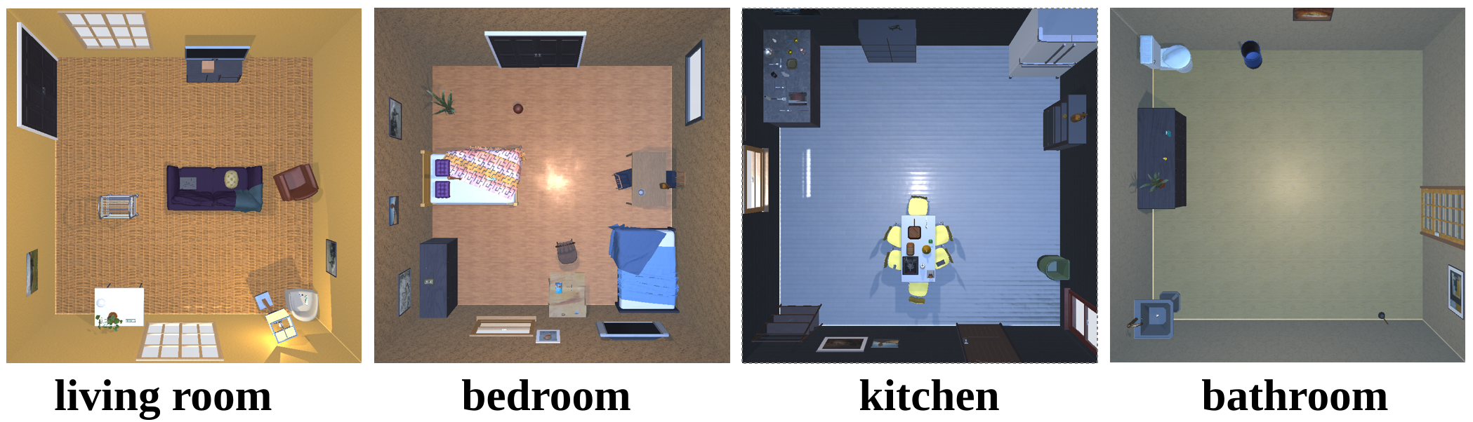
Each room is uniformly square-shaped, enclosed by four walls (north, south, east, and west) that incorporate elements such as doors and windows. Despite this structural consistency, each room type is distinguished by diverse configurations of household objects.
3.4 Specify Spatial Relationships
We incorporate three types of spatial relations: topological, directional, and distance relations. These are utilized to detail the positioning of objects within rooms () and to define the relationships between objects (). The layout constraints, , are expressed as , and the inter-object constraints, , are formulated as .
3.4.1 Object Layout within Room
We incorporate directional and topological spatial relationships to detail how objects are positioned within rooms.
Directional Relations.
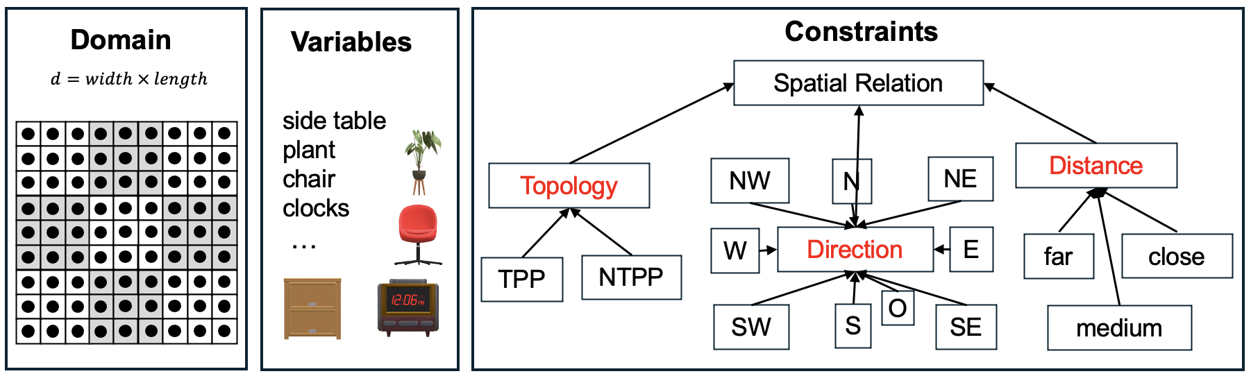
The representation of directional relations between objects extended in 2D space, we just use their central points. As depicted in the left part of Figure 7, we divide the room into nine regions: North (N), West (W), East (E), South (S), Center (C), North-West (NW), North-East (NE), South-West (SW), and South-East (SE). The location of an object in a room is determined by the region in which the centre of its bounding box is situated.
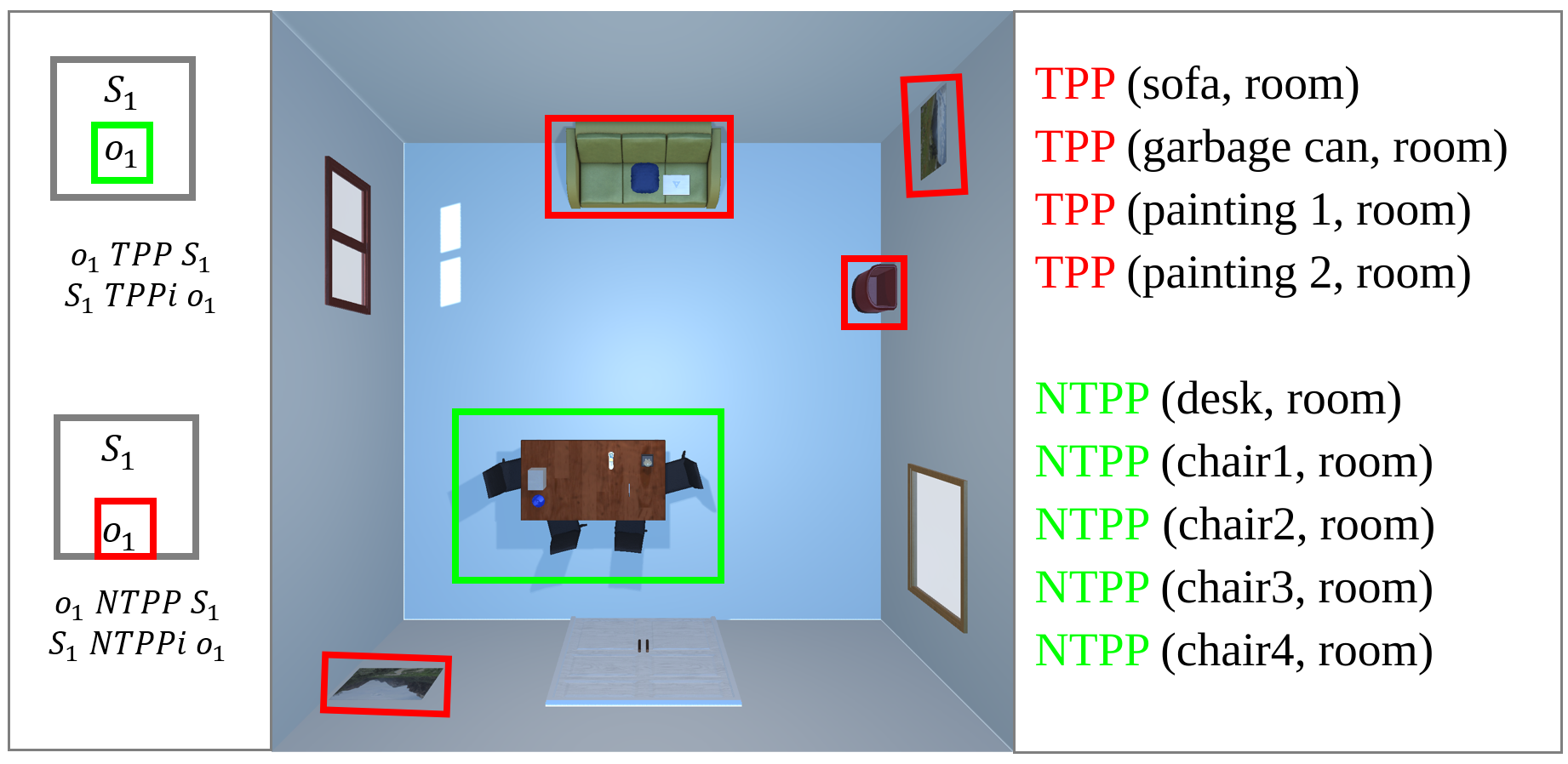
Topological Relations.
Two settings are considered:
-
•
Uniform Inclusion. All objects are considered within the room, with no specific topological distinctions made.
-
•
Tangential Proper Part (TPP) and Non-Tangential Proper Part (NTPP). Just record objects’ topological relations to the wall, not the floor, as depicted in Figure 6.
3.4.2 Relations between Objects
We define the relationships between any two objects using directional and distance-based spatial relations, determined by comparing the and coordinates of their centre points.
Directional Relations.
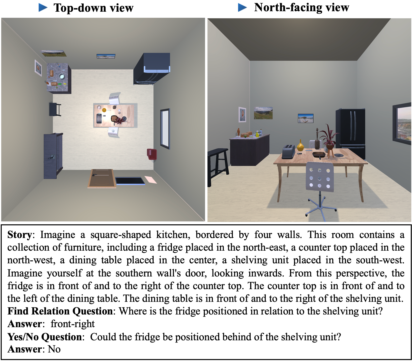
We use a projection-based method to represent the nine different directional relations in cardinal algebra Ligozat (1998), as illustrated in the middle part of Figure 7. We use two reference frames: top-down view and north-facing view, differing in the expression of binary-directional relations. In the top-down view, these relations are depicted using cardinal directions (north, south, east, west) and their combinations. In the facing view, the cardinal directions are adapted to localized terms (front, behind, right, left) to provide a potentially more intuitive understanding of spatial relations from the observer’s viewpoint222It would not be intuitive in the aboriginal language Guugu Yimithirr, which lacks words for ‘left’ or ‘right’, and spatial information is mainly conveyed using cardinal directions Haviland (1998). .
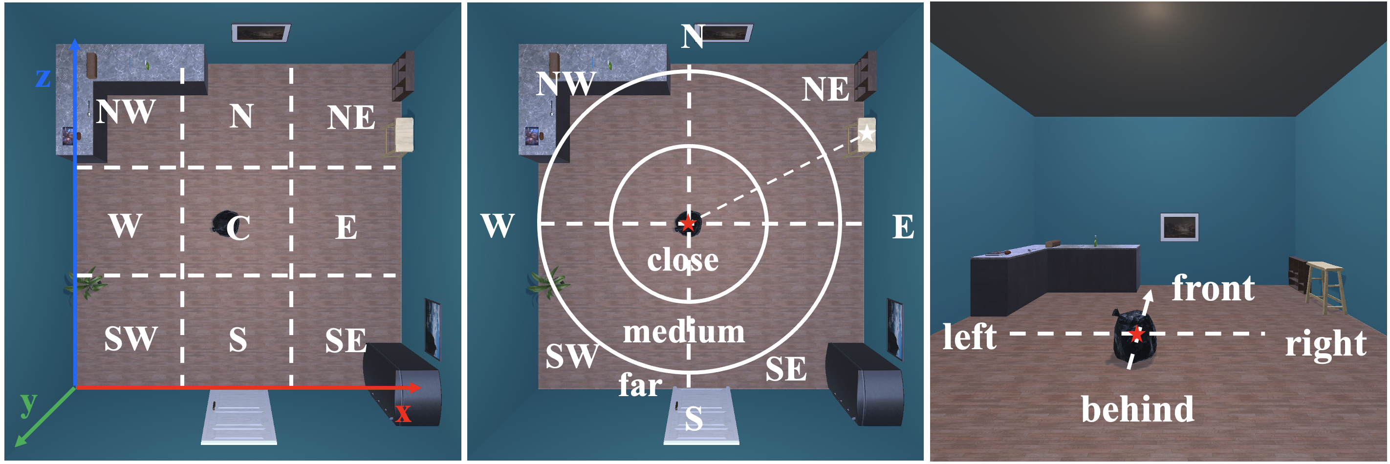
Distance Relations.
The distance between objects is determined by calculating the Euclidean distance between the center points of their bounding boxes . The qualitative distance relations are defined based on the ratio or , where is the length and width of the square room, corresponds to the diagonal length of the room. We have incorporated two levels of distance relation settings in our benchmark:
-
•
close, far (Threshold: ). A binary classification where close is within half the room’s width/length , and far is beyond it, providing a simple distance distinction.
-
•
close, medium, far (Thresholds: , ). The medium category is introduced for a more nuanced understanding, with close up to , medium between and , far beyond , as depicted in the middle part of Figure 7.
3.5 CSP Example Generation
3.5.1 Building a Constraint Graph
Our benchmark offers a variety of stories with varying levels of complexity, accomplished by adjusting two key parameters: for object selection and for constraint determination. Our methodology is implemented as follows:
Node Selection.
We focus on prominent, larger objects that occupy more space in a room. For example, in the context of ‘an apple on a desk’, we would prioritize the desk over the apple. Of the prominent objects in the scene, we randomly select to represent as nodes in the graph.
Constraint Selection.
In a constraint graph with objects, there are potential pair connections. For example, a graph with 5 objects yields possible constraint pairs. For all possible pairs of objects, we first select one pair to form the question. Then, for the remaining pairs, the parameter is used to establish graph.
3.5.2 Answer - Consistency Checking
We include two types of questions: Find Relation (FR): identify the directional spatial relationship between two specified objects. Yes/No (YN): ascertain the validity of a statement concerning the spatial relationship between objects.
Generating ground-truth answers for spatial relations between objects and from the simulation system can be automated through comparing their coordinates, represented as and . However, key considerations arise: Given the stories formed with limited qualitative relations, can we definitively deduce the answer? Is there a possibility of multiple valid solutions? For example, in the scenario ‘A is to the left of B, and C is to the left of A,’ the position of A relative to C is ambiguous based on the information provided. A could be to the right, left, or overlapping with C. The stories in our benchmark offer a partial view of spatial layouts. Given the limited qualitative descriptions, a singular, definitive answer may not always be attainable.
Recognizing the potential for multiple valid solutions within the constraints detailed in the story, we have developed a consistency-checking tool using the python-constraint package333https://github.com/python-constraint/python-constraint, which employs a backtracking algorithm to determine whether a plausible configuration of object relationships can exist to meet all specified constraints. Additional information about this reasoner is available in the Appendix.
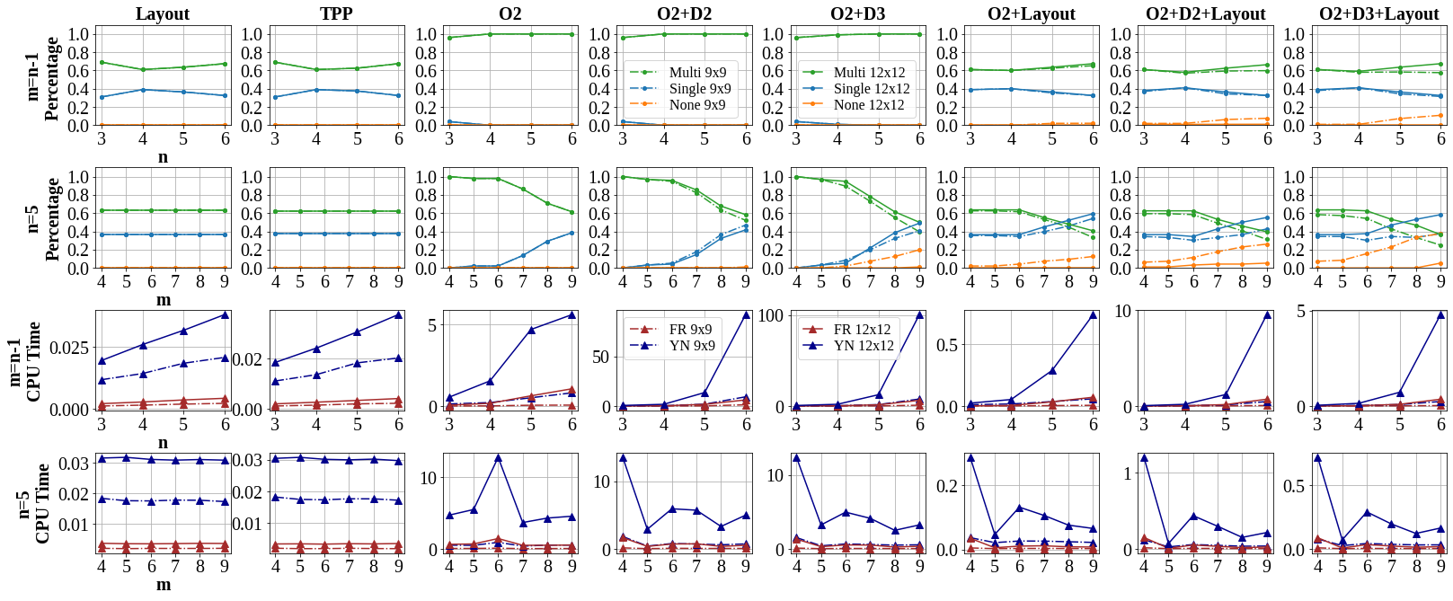
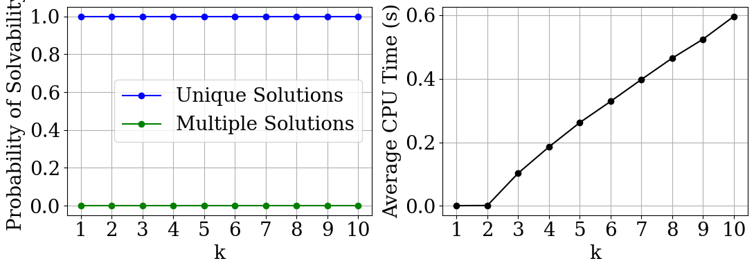
In Figure 8, we analyze the occurrence of single, multiple, and no solution possibilities under various constraint settings. With a smaller domain size of , the Layout and O2 relation settings consistently yield solutions; however, the likelihood of no solution is significantly higher compared to the larger domain size of when incorporating distance constraints. Additionally, the search cost (CPU time) required to find solutions with the larger domain size is considerably higher than with the smaller one. We examine the search costs associated with finding solutions for FR and YN questions. FR questions generally involve multiple answers and require evaluating all nine direction relations to identify all potential solutions that meet the constraints. In contrast, YN questions involve checking only one relational candidate, resulting in lower search costs.
3.6 Generate Textual Descriptions
During this phase, we transform the spatial logical expressions and into natural language sentences and , a process known as logic-to-text generation.
We develop specific logic-to-string templates using context-free grammar (CFG). When forming stories, the logical components such as ,, ,, , are replaced with corresponding textual expressions, enabling the creation of varied descriptions of spatial relationships. Our CFG has two parts, as shown in Table 1.
| This room contains a collection of furniture, including , , …, . |
| . . …. . |
| Imagine yourself at the southern wall’s door, looking inwards. From this perspective, . ….. |
| placed in the , the wall |
| is placed to the of , |
| is , . |
4 Evaluation
4.1 Model Settings and Prompting
We access GPT-3 (Davinci) Brown et al. (2020), GPT-3.5 (Turbo), and GPT-4 OpenAI (2023) via the Azure OpenAI Service, using the API version “2023-09-15-preview” for all three models. To yield more deterministic results, we set the temperature to 0 in all experiments. The remaining parameters were left at the standard configurations for these models.
We conduct experiments with two sets of prompts Bommasani et al. (2021): one set directly presents stories and questions to LLMs, while the other incorporates task descriptions and details about relationship definitions, as detailed in the Appendix, to guide LLMs’ responses.
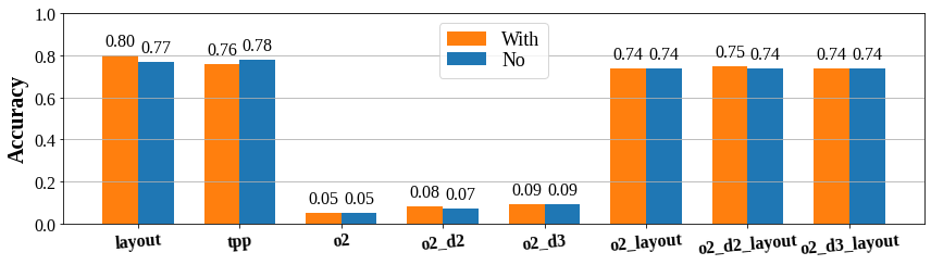
Experiment results (in Appendix) illustrates a slight improvement in the performance of gpt-35-turbo with the Layout, O2+D2, and O2+D2+Layout settings. However, incorporating task description prompts results in a decrease in accuracy within the TPP settings. Therefore, although the added prompts about task description provide valuable insights into the spatial reasoning problem, the minimal variation in performance suggests that for subsequent experiments, we maintain a straightforward story and question format prompt.
4.2 Results
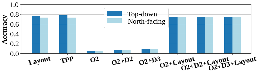
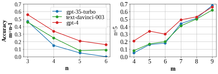
Figure 9 and Figure 10 present the comparative results across models, relation settings, parameters and , highlighting several key observations:
Model Comparison.
GPT-4 consistently surpasses both Turbo and Davinci in nearly all categories and from various viewpoints. Turbo shows comparatively lower accuracy than the other two models, with its accuracy falling to zero under the condition where and .
Viewing Perspective Influence.
The north-facing view descriptions do not significantly impact the results when the narrative already includes descriptions from that view, as in the O2 setting and its combinations with distance or layout, where accuracy remains comparable to the top-down view. However, under the Layout setting, which includes directional descriptions from the top-down view, introducing north-facing view descriptions in the questions complicates comprehension for LLMs, leading to a decline in accuracy.
Impact of Spatial Reasoning Settings.
Layout vs. O2: In the Layout setting, the introduction of TPP does not markedly affect accuracy. Even with , GPT consistently performs well, efficiently extracting and analyzing information. However, when dealing with only the relationships between objects in multi-object scenes, the task becomes challenging for GPT, highlighting the model’s limitations in multi-hop spatial reasoning.
Distance Settings (D2, D3): Interestingly, Turbo’s performance slightly improves with the introduction of distance constraints. This may suggest GPT-4’s better handling of more complex spatial relations.
Combination of Layout, O2 and Distance: The combined settings typically yield performance that is on par with the best-performing individual setting, in this instance, aligning with the results observed in the layout setting.
Variation with Parameters ( and ).
There is a decline in accuracy as increases from 3 to 7, suggesting that larger values create more complex and challenging scenarios (see Figure 10, left). This trend aligns with the observations in Figure 8 - the time taken by the CPU to find solutions increases with higher values. In terms of , an increase in this parameter generally leads to improved accuracy (see Figure 10, right). It appears that larger values, with more densely interlinked spatial relationships, though adding text length, tend to enhance LMs’ performance.
Conclusion
Our study identifies gaps in current QSR datasets and presents a new benchmark to better evaluate LMs’ capabilities in spatial reasoning. We enhance QSR dataset creation with a benchmark that addresses multiple complexities, including topological, directional, and distance relationships. Our benchmark uniquely incorporates different viewing perspectives in spatial reasoning, moving towards more accurate LM evaluations. Our results underscore the necessity for enhancements in current state-of-the-art LLMs, opening new avenues for enhancing spatial reasoning in AI models.
Future directions include incorporating object size and shape, as our current focus is on object centers for spatial relationships. Additionally, exploring more topological relations beyond TPP and NTPP can deepen the benchmark’s scope. We also aim to include more complex perspectives, such as an agent’s viewpoint within a room, introducing natural front-facing scenarios for more challenging reasoning tasks.
This paper provides a preliminary evaluation of OpenAI’s GPT series models on our new dataset RoomSpace-100. Expanding this research to assess and compare the spatial reasoning abilities of other LLMs would be beneficial. Additionally, although our benchmark covers both FR and YN questions, our evaluation is limited to the YN questions. FR questions, which typically require multiple-choice answers, represent a more significant challenge. Future research could delve into these more intricate scenarios. Moreover, while our evaluations utilize RoomSpace-100, exploring larger sets, such as the 1K and 10K versions, could provide more comprehensive insights.
Acknowledgments
We thanks the anonymous referees for their helpful comments. This work has been partially supported by: (1) Microsoft Research - Accelerating Foundation Models Research program, with the provision of Azure resources to access GPT; (2) the Turing’s Defence and Security programme through a partnership with the UK government in accordance with the framework agreement between GCHQ and The Alan Turing Institute; (3) Economic and Social Research Council (ESRC) under grant ES/W003473/1.
Data Access Statement
Data associated with this paper are available from the University of Leeds data repository https://doi.org/10.5518/1518. Code and appendix are available at https://github.com/Fangjun-Li/RoomSpace.
Author Contributions
AC conceived the original idea for the benchmark which was then refined in discussions with FJ and DH. FJ implemented the benchmark and designed all details, performed the evaluations, and wrote the original draft of the paper. All authors contributed to the subsequent drafts.
References
- Alomari et al. [2022] Muhannad Alomari, Fangjun Li, David C Hogg, and Anthony G Cohn. Online perceptual learning and natural language acquisition for autonomous robots. Artificial Intelligence, 303:103637, 2022.
- Bang et al. [2023] Yejin Bang, Samuel Cahyawijaya, Nayeon Lee, Wenliang Dai, Dan Su, Bryan Wilie, Holy Lovenia, Ziwei Ji, Tiezheng Yu, Willy Chung, et al. A multitask, multilingual, multimodal evaluation of ChatGPT on reasoning, hallucination, and interactivity. arXiv preprint arXiv:2302.04023, 2023.
- Bommasani et al. [2021] Rishi Bommasani, Drew A Hudson, Ehsan Adeli, Russ Altman, Simran Arora, Sydney von Arx, Michael S Bernstein, Jeannette Bohg, Antoine Bosselut, Emma Brunskill, et al. On the opportunities and risks of foundation models. arXiv preprint arXiv:2108.07258, 2021.
- Brown et al. [2020] Tom Brown, Benjamin Mann, Nick Ryder, Melanie Subbiah, Jared D Kaplan, Prafulla Dhariwal, Arvind Neelakantan, Pranav Shyam, Girish Sastry, Amanda Askell, et al. Language models are few-shot learners. Advances in neural information processing systems, 33:1877–1901, 2020.
- Cohn and Hernandez-Orallo [2023] Anthony G Cohn and Jose Hernandez-Orallo. Dialectical language model evaluation: An initial appraisal of the commonsense spatial reasoning abilities of LLMs. arXiv preprint arXiv:2304.11164, 2023.
- Cohn and Renz [2008] Anthony G Cohn and Jochen Renz. Qualitative spatial representation and reasoning. In Frank Van Harmelen, Vladimir Lifschitz, and Bruce Porter, editors, Handbook of knowledge representation, pages 551–596. Elsevier, 2008.
- Deitke et al. [2022] Matt Deitke, Eli VanderBilt, Alvaro Herrasti, Luca Weihs, Kiana Ehsani, Jordi Salvador, et al. Procthor: Large-scale embodied ai using procedural generation. Advances in Neural Information Processing Systems, 35:5982–5994, 2022.
- Haviland [1998] J B Haviland. Guugu Yimithirr cardinal directions. Ethos, 26(1):25–47, 1998.
- Li et al. [2022] Fangjun Li, DC Hogg, and AG Cohn. Ontology knowledge-enhanced in-context learning for action-effect prediction. Advances in Cognitive Systems. ACS-2022, 2022.
- Li et al. [2024] Fangjun Li, David C Hogg, and Anthony G Cohn. Advancing spatial reasoning in large language models: An in-depth evaluation and enhancement using the stepgame benchmark. In Proceedings of the AAAI Conference on Artificial Intelligence, volume 38, pages 18500–18507, 2024.
- Ligozat [1998] Gerard Ligozat. Reasoning about cardinal directions. Journal of Visual Languages & Computing, 9(1):23–44, 1998.
- Mirzaee and Kordjamshidi [2022] Roshanak Mirzaee and Parisa Kordjamshidi. Transfer learning with synthetic corpora for spatial role labeling and reasoning. In Proceedings of the 2022 Conference on Empirical Methods in Natural Language Processing, pages 6148–6165. Association for Computational Linguistics, December 2022.
- Mirzaee et al. [2021] Roshanak Mirzaee, Hossein Rajaby Faghihi, Qiang Ning, and Parisa Kordjamshidi. SpartQA: a textual question answering benchmark for spatial reasoning. In Proceedings of the 2021 Conference of the North American Chapter of the Association for Computational Linguistics: Human Language Technologies, pages 4582–4598, 2021.
- OpenAI [2023] OpenAI. GPT-4 technical report. ArXiv, abs/2303.08774, 2023.
- Randell et al. [1992] David A Randell, Zhan Cui, and Anthony G Cohn. A spatial logic based on regions and connection. KR, 92:165–176, 1992.
- Shi et al. [2022] Zhengxiang Shi, Qiang Zhang, and Aldo Lipani. Stepgame: A new benchmark for robust multi-hop spatial reasoning in texts. In Proceedings of the AAAI conference on Artificial Intelligence, volume 36, pages 11321–11329, 2022.
- Touvron et al. [2023] Hugo Touvron, Louis Martin, Kevin Stone, Peter Albert, et al. Llama 2: Open foundation and fine-tuned chat models, 2023.
- Weston et al. [2016] Jason Weston, Antoine Bordes, Sumit Chopra, Alexander M Rush, Bart Van Merriënboer, Armand Joulin, and Tomas Mikolov. Towards AI-complete question answering: A set of prerequisite toy tasks. In 4th International Conference on Learning Representations, ICLR, 2016.
Appendix A Existing Benchmarks
| bAbI | StepGame | SpartQA | |
| Represent | Grid-based (point) | shape-based | |
| object type | color+shape(T17), location(T19) | A-Z | shape + size + color |
| relation | relative(T17), cardinal(T19) | relative, cardinal | cardinal, distance, RCC, |
| constraint | unit distance and angle | relation defination | |
| description | templates | templates | CFG |
| Images | No | Yes, but not matching the story’s objects. | |
Appendix B Logical Reasoner for Consistency Checking
Our CSP is represented in terms of variables (objects), finite room domains, and constraints (spatial relation sets).
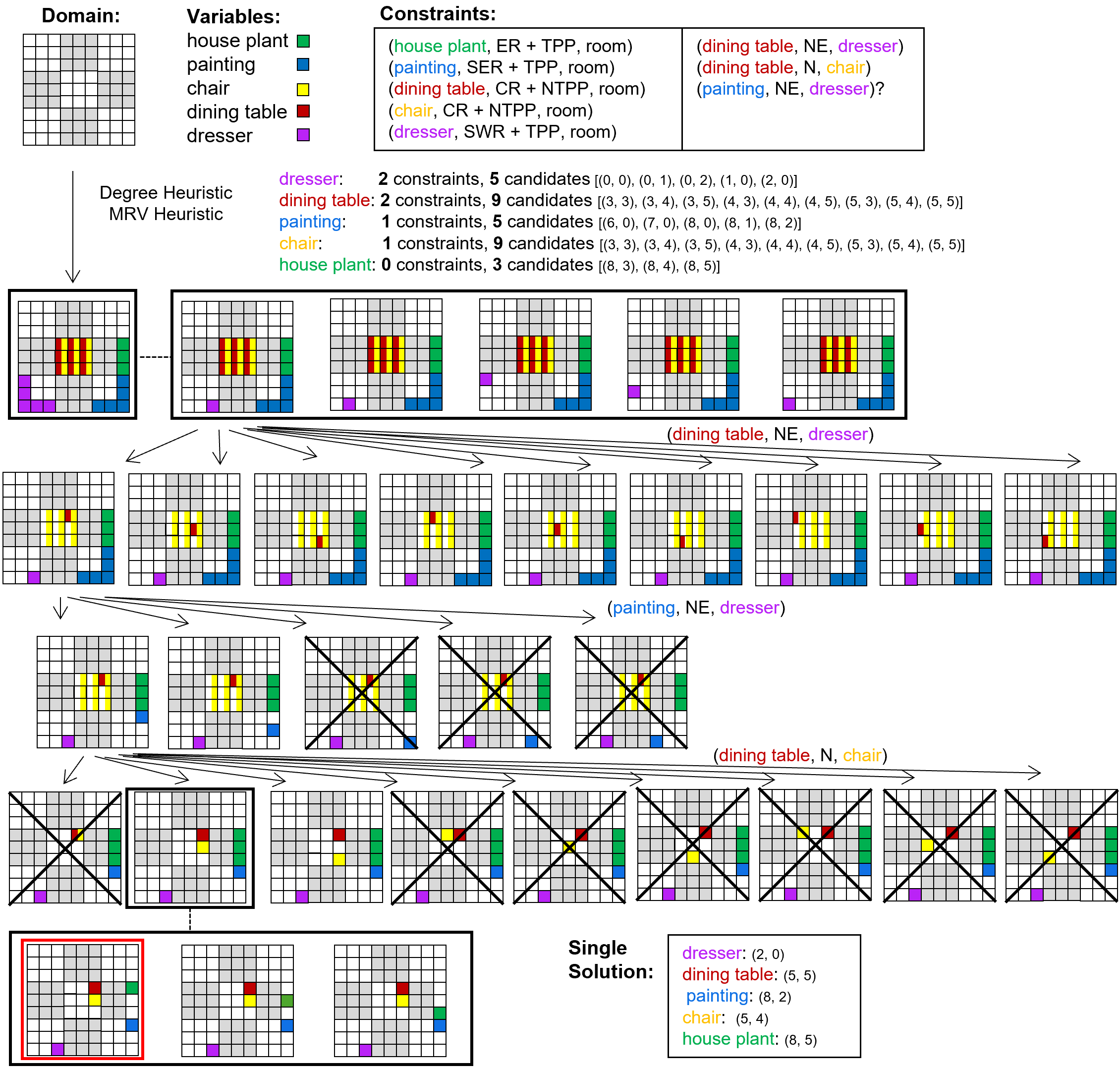
We use the backtracking algorithm for solving our CSP, where the goal is to find an assignment of values to variables that satisfies all given constraints. Here is a summary of how the algorithm works:
-
1.
Variable Selection: Employs a combination of the Degree Heuristic (prioritize variables with the most constraints on remaining variables) and the Minimum Remaining Values (MRV) heuristic (prioritize variables with the fewest legal values left) to choose the next variable to assign. This helps in reducing the search space and picking the most constrained variable first.
-
2.
Value Selection and Forward Checking: For the selected variable, iterate through its possible values (domain). Forward checking tentatively assigns a value and checks if this leads to any immediate dead ends in the remaining variables (i.e., if any variable is left with no possible values), which helps in pruning the search space early.
-
3.
Constraint Checking: For each value attempted, check all relevant constraints. If a value does not satisfy a constraint, it is discarded, and the algorithm tries the next value. If all values are tried and none fits, backtrack to the previous variable and try a new value for it, undoing any changes made since that variable was assigned.
-
4.
Solution Yielding and Backtracking: Once all variables are assigned in a way that all constraints are satisfied, a solution is yielded. If the solution space is exhausted for the current path, backtrack to explore other paths.
B.1 Complexity
The time complexity of backtracking algorithms for CSPs can vary significantly based on the problem’s constraints, the size of the domains and variables, and the heuristics used:
Worst-Case Time Complexity: In the worst case, the algorithm might explore every possible assignment of values to variables, leading to a time complexity of , where is the size of the largest domain, and is the number of variables.
B.2 Influence of Constraints
The number and type of constraints significantly affect the complexity of solving a CSP. Here is how constraints can impact the complexity:
Tightness: This refers to how restrictive a constraint is. A tighter constraint eliminates more values from the domains of the variables it involves. To illustrate, consider the constraint (house plant, ER, room) applied to the variable ‘house plant’ within a domain of possibilities. Introducing constraint (house plant, ER+TPP, room) further reduces the domain to only 5 possible pairs: [(0, 0), (0, 1), (0, 2), (1, 0), (2, 0)]. This is the reason, as depicted in Figure 8, that there is a marked decrease in CPU times when we transition from a ‘Layout’ configuration to a ‘TPP’ setting.
Tighter constraints can reduce the search space because fewer value combinations are valid, but they also increase the chance of running into a dead end (where no solution is possible), which can force more backtracking. Figure 8 demonstrates that incorporating binary distance relations ‘O2+D2’ leads to a rise in the average CPU time when contrasted with the ‘O2’ configuration.
We provide an analysis of the constraint tightness for all spatial relations. In our CSP solver, we explore two settings for domain size: and , corresponding to the room’s square configuration.
Layout Constraints: These constraints are not represented in constraint graphs; rather, they are utilized directly to refine the domain of the variable they constrain. Though in the form , they function as unary constraints.
-
•
InR (In Room): , all possible values from the domain of the one variable are allowed and the constraint is always satisfied.
-
•
NR, SR, WR, ER, NER, NWR, SER, SWR, CR: , Each relation pertains to a specific section of the room, dividing the room into nine parts.
-
•
TPP, NTPP: TPP corresponds to the border of the grid space, with , NTPP corresponds to the inner side of the room, with
Inter-Objects Constraints: We use binary constraints involving two variables to represent the relationships between objects, which can be illustrated in constraint graphs.
-
•
N, S, W, E, NE, NW, SE, SWR, O: Directions between Objects. For N, S, W, E, , for NE, NW, SE, SWR, . For O,
-
•
CL2, FR2: Objects are considered close (CL2) if they are within half of the maximum distances for one dimension (width or length). We approximate this using a circle with radius , so , The calculation for distance in terms of the grid dimension is complex. The number of cells within this area () for the central object can be approximated by: , . For each central object, the actual count of possible variable values is limited by the number of cells that fit into this area.
-
•
CL3, MD3, FR3: more restrictive than the previous two-category distances. Objects are considered close (CL3) if they are within one-third of the maximum distances within the grid, and moderate distance (MD3) if within two-thirds of the maximum distances within the grid. We approximate this using a circle with radius , . , .
, .
Density: This is about the number of constraints in the problem relative to the number of variables, aligning with in Figure 8. A higher density means more pairs of variables are constrained relative to each other. More constraints generally increase the complexity because more conditions must be satisfied, potentially increasing the amount of backtracking required.
In Figure 8, There is a rising curve of CPU times as increases across all six relational configurations. Theoretically, the worst-case time complexity is expected to escalate exponentially. However, due to forward checking and the use of MRV and Degree heuristics, the effective branching factor is often significantly reduced, leading to much better performance in practice.
Appendix C Prompt Design
The prompts mentioned in Section 4.1 were designed to clarify spatial relations, reducing ambiguity in spatial descriptions. For different sets of spatial reasoning problems, corresponding guidelines will be combined with the task description part to form the prompt.
-
•
Task: Analyze the spatial relationships between specified objects in a room, treating each object as a point within a 1212 grid.
-
•
Distance-2: Distances between objects in the room are determined using the room’s width. A ‘short distance’ is defined as any distance up to half of the room’s width. A ‘far distance’ refers to any distance that exceeds half of the room’s width.
-
•
Distance-3: Distances between objects in the room are determined based on the room’s diagonal length. A ‘short distance’ refers to a distance that is up to one-third of the diagonal. A ‘moderate distance’ spans from one-third to two-thirds of the diagonal. A ‘far distance’ is any distance that exceeds two-thirds of the diagonal.