ElastoGen: 4D Generative Elastodynamics

Abstract

We present ElastoGen, a knowledge-driven model that generates physically accurate and coherent 4D elastodynamics. Instead of relying on petabyte-scale data-driven learning, ElastoGen leverages the principles of physics-in-the-loop and learns from established physical knowledge, such as partial differential equations and their numerical solutions. The core idea of ElastoGen is converting the global differential operator, corresponding to the nonlinear elastodynamic equations, into iterative local convolution-like operations, which naturally fit modern neural networks. Each network module is specifically designed to support this goal rather than functioning as a black box. As a result, ElastoGen is exceptionally lightweight in terms of both training requirements and network scale. Additionally, due to its alignment with physical procedures, ElastoGen efficiently generates accurate dynamics for a wide range of hyperelastic materials and can be easily integrated with upstream and downstream deep modules to enable end-to-end 4D generation.

1 Introduction

Recent advancements in generative models have enhanced the ability to produce high-quality samples across diverse media formats (e.g. images, videos, 3D models, 4D data). In particular, the generation of 4D data, including both spatial and temporal dimensions, has seen notable progress [62, 60, 69, 42, 3, 72, 4].

However, learning physical dynamics that exhibit temporal consistency and adhere to physical laws from observable data is a difficult task. Data are in the wild and noisy. Their underlying coherence is agnostic to the user. As a result, existing deep models have to assume some distributions of the data, which may not be the case in reality. In theory, the network would extract any knowledge provided sufficient data. In practice however, such data-based learning becomes more and more cumbersome with increased dimensionality of generated contents – it is unintuitive to define the right network structure to guide the physically meaningful generation; it requires terabyte- or petabyte-scale high-quality training data; and center-level computing resource to facilitate the training. Those theoretical and practical obstacles combined impose significant challenges.

We explore a new way to establish physics-in-the-loop generative models. Our argument is that learning from knowledge instead of raw data is more effective for generative models. Many physical laws and principles are mathematically in the form of partial differential equations (PDEs) and are numerically solved with discretized differential operators. We note that those operators hold a similar structure as a convolution kernel on the problem domain, where the values of those convolution kernels depend on the specific problem setting. Inspired by those observations, we propose ElastoGen, a knowledge-driven neural model that generates physically accurate and coherent 4D elastodynamics. ElasoGen can be easily coupled and integrated with upstream and downstream neural modules to enable end-to-end 4D generation. The core idea of ElastoGen is converting the global differential operator, corresponding to the nonlinear elastodynamic equations, into iterative local convolution-like operations, which naturally fit modern deep networks. Each network module has a clear purpose rather than being part of a black box. As a result, ElasoGen is super lightweight – in terms of both training and the network scales. Furthermore, due to its consistency with physics procedure, ElastoGen efficiently generates accurate dynamics for a wide range of hyperelastic materials. Key contributions of ElastoGen include:

Compact generative network inspired by physics law. ElastoGen does not rely on large datasets. Instead, it uses physical laws and computational physics knowledge to design a network structure that decouples various modules and remains compact and efficient. After lightweight training, ElastoGen accurately generates physical dynamics by solving the weak form of governing PDEs.

Neural Metric with Diffusion-Based Parameterization. ElastoGen introduces a neural metric to handle hyperelastic materials, generating dynamics for materials like Neo-Hookean and StVK. Using diffusion models, it efficiently produces network parameters that accurately respond to physical parameters, enhancing the versatility and accuracy of dynamics.

General subspace method for efficient matrix-free computation. ElastoGen introduces a general subspace method. This method efficiently extracts low-frequency dynamics and uses a few Jacobi iterations to restore high-frequency dynamics, making the computation matrix-free and improving the efficiency of dynamic generation.

2 Related Work

Generative models The primary objective of generative models is to produce new, high-quality samples from vast datasets. These models are designed to learn and understand the distribution of data, thereby generating samples that meet specific criteria. Techniques such as Generative Adversarial Networks (GANs) [21], Variational Autoencoders (VAEs) [34], and flow-based methods [14, 15] have all demonstrated significant success. However, each method has its limitations. For instance, GANs can generate high-quality images but are notoriously difficult to train and optimize [2, 22, 47]. VAEs [65, 12] and flow-based methods [33] offer efficient training processes but generally fall short in sample quality compared to GANs. Recently, diffusion models have emerged as another powerful technique, achieving state-of-the-art results in generating high-fidelity images [63, 24, 58], setting the stage for further explorations in more complex applications.

4D Generation based on Diffusion Models As research on diffusion models advances, these methods could potentially be applied to the generation of 3D content [29, 41, 48, 55, 66, 44, 43], video content [7, 23, 26, 25, 31, 53], and more complex forms such as 3D videos or what might be termed 4D scenes [62, 60, 69, 42, 3, 72, 4]. These advanced applications demonstrate the versatility and expanding potential of diffusion models across diverse media formats. However, existing video generation techniques struggle to ensure temporal consistency and require substantial training data, underscoring the challenges of capturing and replicating the dynamic and interconnected behaviors present in real-world scenarios within a generative model framework.

Neural Physical Dynamics Physical dynamics traditionally relies on numerical solutions such as the finite element method (FEM) [75, 76, 27, 57], finite difference method [74, 20], or mass-spring systems [45]. Each approach offers distinct advantages and limitations. For example, Position-Based Dynamics (PBD) [51] and Projective Dynamics (PD) [8, 45] offer simplified implementation and faster convergence but can struggle with complex material behaviors and do not always guarantee consistent convergence rates. Recently, neural physics solvers, which integrate neural networks with traditional solvers, aim to accelerate and simplify the computation process. The pioneering works [11, 6] directly utilized neural networks to predict dynamics, achieving promising results in simple particle systems. Subsequent studies [59, 35, 1, 40, 38, 39] adopted network architectures to the specific features of the systems, thereby enhancing performance. The advent of Physics Informed Neural Networks (PINNs) [56, 54] marks a leap forward. These networks incorporate extensive physical information to constrain and guide the learning process, ensuring that predictions adhere more closely to physical laws and has succeeded in domains such as cloths [18] and fluids [64, 19, 13]. Some work [71] shifts away from end-to-end structures and use neural networks to optimize part of the simulation. Another line of research generates dynamics through physics-based simulators, where network learns static information while physical laws govern the generation of dynamics [37, 16, 68, 17, 30], giving physical meanings to Neural Radiance Fields (NeRF) [49, 32]. These methods demonstrate the benefits of embedding human knowledge into networks to reduce the learning burden.

3 Background

To be self-contained, we start with a brief review of core techniques on which our pipeline is built.

3.1 Nonlinear elastodynamic

Based on the classical Lagrangian mechanics [52], the dynamic equilibrium of a 3D model is characterized as $\frac{\mathrm{d}}{\mathrm{d}t}\left(\frac{\partial L}{\partial\dot{\mathbf{q}}}\right)-\frac{\partial L}{\partial\mathbf{q}}=\mathbf{f}_{q}$, where $L=T-U$ is Lagrangian i.e., the difference between the kinematic energy ($T$) and the potential energy ($U$) of the system. $\mathbf{q}$ and $\dot{\mathbf{q}}$ are generalized coordinate and velocity. $\mathbf{f}_{q}$ is the generalized external force. When using the implicit Euler time integration scheme: $\mathbf{q}_{n+1}=\mathbf{q}_{n}+h\dot{\mathbf{q}}_{n+1}$, $\dot{\mathbf{q}}_{n+1}=\dot{\mathbf{q}}_{n}+h\ddot{\mathbf{q}}_{n+1}$, it can be reformulated as a nonlinear optimization problem to be solved at each time step:

$$\mathbf{q}_{n+1}=\underset{\mathbf{q}}{\mathrm{argmin}}\left\{\frac{1}{2h^{2}}\|\mathbf{q}-\mathbf{q}_{n}-h\dot{\mathbf{q}}_{n}\|^{2}_{\mathbf{M}}-\mathbf{q}^{\top}\mathbf{f}_{q}+U(\mathbf{q})\right\},$$ (1)

where the subscript of $\mathbf{q}$ indicates the timestep index, $h$ is the timestep size and $\mathbf{M}$ is the mass matrix.

3.2 Diffusion model

Diffusion models transform a probability from a real data distribution $\mathcal{P}_{\text{real}}$ to a target distribution $\mathcal{P}_{\text{target}}$ through two processes: diffusion and denoising.

Diffusion: This process incrementally adds Gaussian noise to the initial data $\mathbf{x}_{0}\sim\mathcal{P}_{\text{target}}$, gradually transforming it into a sequence $\mathbf{x}_{1},\mathbf{x}_{2},...,\mathbf{x}_{T}$, where $\mathbf{x}_{T}$ approximates the real distribution $\mathcal{P}_{\text{real}}$. The aim is to learn a noise prediction model $\boldsymbol{\epsilon}_{\theta}(\mathbf{x}_{t},t)$, estimating the noise at each step $t$ to facilitate data recovery in the denoising phase. The noise learning objective is formulated as:

$$L=\mathbb{E}_{\mathbf{x}_{0}\sim\mathcal{P}_{\text{target}},\boldsymbol{\epsilon}\sim\mathcal{N}(\mathbf{0},\mathbf{I}),t\sim\text{Uniform}(\{1,...,T\})}[\|\boldsymbol{\epsilon}-\boldsymbol{\epsilon}_{\theta}(\mathbf{x}_{t},t)\|^{2}_{2}],$$ (2)

where $\|\cdot\|_{2}^{2}$ denotes the mean squared error loss.

Denoising: This reverse process iteratively removes noise from $\mathbf{x}_{T}\sim\mathcal{P}_{\text{real}}$, recovering the original data $\mathbf{x}_{0}$ by adjusting the noisy data at each time $t$ as:

$$\mathbf{x}_{t-1}=\frac{1}{\sqrt{\alpha_{t}}}(\mathbf{x}_{t}-\frac{1-\alpha_{t}}{\sqrt{(1-\overline{\alpha}_{t})}}\boldsymbol{\epsilon}_{\theta}(\mathbf{x}_{t},t))+\sigma_{t}\mathbf{z},\quad\mathbf{z}\sim\mathcal{N}(\mathbf{0},\mathbf{I}),$$ (3)

where $1-\alpha_{t}:=\beta_{t}$ is a scheduled variance at time $t$, and $\sigma_{t}$ is typically set to $\sigma_{t}=\sqrt{\beta_{t}}$.

These processes allow modeling the transition between distributions effectively, using learned Gaussian transitions for noise prediction and reduction.

4 Methodology

As shown in Fig. 1, ElastoGen uses physical parameters to guide the generation of network weights through a diffusion model. It takes a voxelized 3D model and its boundary conditions as inputs, and by iteratively performing alternating local and global optimizations, it accurately computes the physics-based elastic dynamics of the object. Adhering to physical laws and inspired by computational physics knowledge, our network architecture achieves remarkable results with minimal parameterization and lightweight training. Additionally, our model can handle hyperelastic material accurately. In the following sections, we will provide detailed explanations of the major steps in the pipeline.

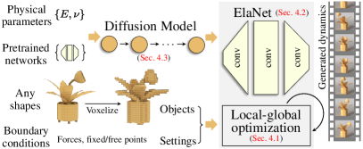
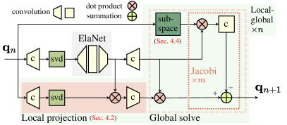
(a) The pipeline of ElastoGen.	(b) The network structure.

Figure 1: ElastoGen overview.  (a) ElastoGen inputs a voxelized 3D model and boundary conditions, using physical parameters to generate ElaNet’s weights via a diffusion model. ElaNet performs local and global optimizations to compute elastic dynamics. (b) Adhering to physical laws, our architecture achieves accurate dynamics for hyperelastic materials with minimal parameterization. The network updates from $\mathbf{q}_{n}$ to $\mathbf{q}_{n+1}$ using ElaNet for local projections and global solving.

4.1 Elastodynamics generator

Numerical methods solve the weak form of Eq. (1), where its derivative equals zero. This invariably involves solving a large linear system $\mathbf{A}\mathbf{x}=\mathbf{b}$. For instance, in Newton’s method, $\mathbf{A}$ represents the Hessian of Eq. (1), which changes per iteration. In contrast, PD splits the optimization into local and global steps by introducing auxiliary variables, making $\mathbf{A}$ constant and allowing for pre-decomposition techniques to accelerate the process. Generally, any existing numerical method for solving Eq. (1) can guide the architecture of our elastodynamics generator. We primarily base our network design on the principles of PD due to its efficiency and ease of implementation.

PD expresses the nonlinear energy $U$ as a sum of multiple quadratic terms, defined by $U(\mathbf{q})=\sum_{i}E_{i}(\mathbf{q})$. Here, each term $E_{i}(\mathbf{q})=\underset{\mathbf{p}_{i}\in\mathcal{M}_{i}}{\min}\frac{\omega_{i}}{2}\left\|\mathbf{q}\mathbf{G}_{i}-\mathbf{p}_{i}\right\|^{2}$, where $i$ represents the $i$-th element, $E_{i}$ represents the elastic energy of the element and $\mathbf{G}_{i}$ is a discrete differential operator. For a tetrahedral mesh, the deformation gradient $\mathbf{F}_{i}(\mathbf{q})=\mathbf{q}\mathbf{G}_{i}$ [61]. With this quadratic asssumption, the large nonlinear optimization problem in Eq.(1) is simplified to performing local-global iterations until convergence. Each iteration alternates between two phases: a local phase to project each element independently to satisfy its specific constraints:

$$E_{i}(\mathbf{q})=\underset{\mathbf{p}_{i}\in\mathcal{M}_{i}}{\min}\frac{\omega_{i}}{2}\|\mathbf{F}_{i}(\mathbf{q})-\mathbf{p}_{i}\|^{2}$$ (4)

and a global phase to solve a quadratic optimization that considers all elements:

$$\mathbf{q}_{n+1}=\underset{\mathbf{q}}{\mathrm{argmin}}\left\{\frac{1}{2h^{2}}\|\mathbf{q}-\mathbf{q}_{n}-h\dot{\mathbf{q}}_{n}\|^{2}_{\mathbf{M}}-\mathbf{q}^{\top}\mathbf{f}_{\mathbf{q}}+\sum_{i}E_{i}(\mathbf{q})\right\}$$ (5)

The constraint manifold $\mathcal{M}_{i}$ is the zero level set of the elastic energy of the $i$-th element, making the auxiliary variable $\mathbf{p}_{i}$ a projection of $\mathbf{F}_{i}(\mathbf{x})$ onto $\mathcal{M}_{i}$. For more implementation details of PD, we refer the readers to this paper [8].

As explained in paper  [46], PD approximates the elastic energy function by constructing appropriate manifolds $\mathcal{M}_{i}$ and weights $\omega_{i}$. However, this method struggles to achieve plausible results for non-quadratic elastic models. ElastoGen adopts the principles of PD, utilizing neural networks to efficiently collect local information and a global solver to integrate the local information. We design a neural network architecture based on PD’s computational model, allowing the original problem to be divided into multiple smaller problems that can be trained separately. Notably, our network architecture design approach can be applied to any numerical method and is not limited to PD. This design approach significantly reduces the coupling between different modules, breaking down the overall training process into multiple lightweight training modules and greatly reducing the need for large amounts of data. Based on this idea, we will focus on introducing the design principles of each module. For detailed implementations and training methods, please refer to the appendix.

4.2 Neural metric local projection

In the original formulation of the local step, the Frobenius norm is used as the distance metric, which limits itself to measuring quadratic energies. Here, we propose using a neural metric to enhance the expressiveness of this metric while preserving its desirable properties. For a tetrahedral mesh, our metric is formulated as:

$$E(\mathbf{F})=\underset{\mathbf{p}\in\mathcal{SO}(3)}{\mathrm{argmin}}\frac{\omega}{2}\|\mathbf{F}\mathbf{N}(\mathbf{F})-\mathbf{p}\|^{2}.$$ (6)

Here, $\omega$ is calculated as $\omega={E}/({2(1+\nu)})$ with Young’s modulus $E$ and Poisson’s ratio $\nu$. $\mathbf{F}$ is the deformation gradient of each tetrahedron, and $\mathbf{N}(\mathbf{F})$ is the neural network we call ElaNet (as in Fig. 1), with $\mathbf{F}$ as the input. As shown in the left inset, ElaNet projects $\mathbf{F}$ to a point $\mathbf{F}\mathbf{N}(\mathbf{F})$ on the line passing through $\mathbf{F}$ and its projection $\mathbf{F}_{\text{proj}}$ on the manifold $\mathcal{M}$. This new point is positioned in the way that its distance to the manifold approximates a desired energy model.

Additionally, useful elastic models should exhibit rotational invariance, where the energy remains zero when an object rotates without shape changes. Therefore, we choose $\mathcal{M}=\mathcal{SO}(3)$, with $\mathcal{SO}(3)$ being the 3D rotation group, in our neural metric. For isotropic elastic models, the energy depends only on the magnitudes of the three singular values of $\mathbf{F}$ and is independent of their order. Assuming that the singular value decomposition of the deformation gradient is $\mathbf{F}=\mathbf{U}\mathbf{S}\mathbf{V}^{\top}$, where $\mathbf{S}$ is a diagonal matrix with singular values arranged in descending order, the elastic energy depends solely on $\mathbf{S}$ and is independent of $\mathbf{U}$ and $\mathbf{V}$. Thus, our neural metric should also adhere to this property, and with subscripts omitted, it is reformulated as:

$$\begin{split}E(\mathbf{F})&=\underset{\mathbf{p}\in\mathcal{SO}(3)}{\mathrm{argmin}}\frac{\omega}{2}\|\mathbf{F}\mathbf{N}(\mathbf{F})-\mathbf{p}\|^{2}=\frac{\omega}{2}\|\mathbf{U}\mathbf{S}\mathbf{V}^{\top}\mathbf{N}(\mathbf{F})-\mathbf{U}\mathbf{V}^{\top}\|^{2}\\ &=\frac{\omega}{2}\mathrm{tr}\left(\mathbf{S}\mathbf{S}\mathbf{V}^{\top}\mathbf{N}(\mathbf{F})\mathbf{N}^{\top}(\mathbf{F})\mathbf{V}+\mathbf{I}-2\mathbf{V}\mathbf{S}\mathbf{V}^{\top}\mathbf{N}(\mathbf{F})\right).\end{split}$$ (7)

To ensure $E(\mathbf{F})$ behaves well, we enforce the following two properties. First, $\mathbf{N}(\mathbf{F})$ must be a symmetric matrix, because we require that $\mathbf{F}\mathbf{N}(\mathbf{F})$ has the same projection point on $\mathcal{SO}(3)$ as $\mathbf{F}$. Second, for an isotropic material, $E(\mathbf{F})$ should be a function solely dependent on $\mathbf{S}$. Therefore, we apply transformations to the original network output. Denoting the original network output as $\mathbf{N}_{0}(\mathbf{S})$, we can make it symmetric by letting $\mathbf{N}(\mathbf{F})=\mathbf{V}(\mathbf{N}_{0}(\mathbf{S})+\mathbf{N}_{0}^{\top}(\mathbf{S}))\mathbf{V}^{\top}$. With $\mathbf{Q}(\mathbf{S}):=\mathbf{S}\left(\mathbf{N}_{0}(\mathbf{S})+\mathbf{N}_{0}^{\top}(\mathbf{S})\right)$ defined, Eq. (7) is simplified to be only dependent on $\mathbf{S}$, that is,

$$\begin{split}E(\mathbf{F})=\frac{\omega}{2}\mathrm{tr}\left(\mathbf{Q}(\mathbf{S})\mathbf{Q}^{\top}(\mathbf{S})\right)+\frac{3\omega}{2}-\omega\ \mathrm{tr}\left(\mathbf{Q}(\mathbf{S})\right).\\ \end{split}$$ (8)

Since the local projection operation for each tetrahedron does not affect others’, we can process each local projection in parallel. Our network inputs a voxelized 3D representation, where each voxel is divided consistently into $6$ tetrahedra, thus housing $6$ local projections with identical operations across voxels. This uniformity allows the use of 3D convolution for implementing local projections. We first apply a convolution on the voxels to obtain the deformation gradients of the $6$ tetrahedra within each voxel. Then, we perform parallel $3\times 3$ SVD on all deformation gradients to get $\mathbf{U}$, $\mathbf{V}$ and $\mathbf{S}$. A CNN then computes $\mathbf{N}(\mathbf{F})$ for all voxels, realizing our neural metric local projection. The weights of the convolutional network that calculate the deformation gradients depend only on how the voxel is divided into tetrahedra, and can be pre-trained in advance. This is a simple and lightweight structure (see appendix). In contrast, ElaNet $\mathbf{N}(\mathbf{F})$ must be trained based on physical parameters such as Young’s modulus $E$ and Poisson’s ratio $\nu$.

4.3 Physics-to-neural generation with diffusion

To train the diffusion model, we prepare a dataset of paired $\mathbf{P}$ and $\mathbf{W}$. We first uniformly sample $\mathbf{P}$ at fixed intervals and then establish a topological order, as shown in the left inset. A target elastic energy $\Psi_{\mathbf{P}}$ is then formulated for each sampled $\mathbf{P}$, and $\mathbf{W}$ is optimized as:

$$\qquad\qquad\qquad\qquad\mathbf{W}=\underset{\mathbf{W}}{\mathrm{argmin}}\left\|\log(\frac{\omega}{2}\|\mathbf{F}\mathbf{N}_{\mathbf{W}}(\mathbf{F})-\mathbf{p}\|^{2}+1)-\log(\Psi_{\mathbf{P}}(\mathbf{F})+1)\right\|^{2},$$ (9)

We proceed to generate ElaNet, which takes input as $\mathbf{F}$ and outputs $\mathbf{N}(\mathbf{F})$. $\mathbf{N}(\mathbf{F})$ is then formulated into energy with Eq. 6. Different input physical parameters $\mathbf{P}=\{E,\nu\}$ will result in different $\mathbf{N}(\mathbf{F})$ for the same $\mathbf{F}$, formulating different energies. A straightforward approach is to train a network $\mathbf{N(F,P)}$ directly on $\mathbf{F}$ and $\mathbf{P}$. However, as ElaNet frequently recalculates $\mathbf{N}(\mathbf{F})$ when object deforms and the physical parameter $\mathbf{P}$ remains fixed after initialization, it is more efficient to decouple $\mathbf{N(F)}$ and $\mathbf{P}$ to keep the network compact. Inspired by Zhang et al. [73], we realize that the network $\mathbf{N}(\mathbf{F})$ can be generated using another diffusion network guided by $\mathbf{P}$. Specifically, $\mathbf{W}:=\mathbf{D}(\mathbf{P})$, where $\mathbf{W}$ is the parameters of the network $\mathbf{N}(\mathbf{F})$ and $\mathbf{D}$ is a diffusion model.

where $\mathbf{N}_{\mathbf{W}}$ represents the network with parameter $\mathbf{W}$. We use $\log$ operation given that the energy of some elastic materials change dramatically with deformation and that the energy is always non-negative. Since the elastic energy function itself changes smoothly with $\mathbf{P}$, $\mathbf{W}$ can converge within only hundreds of gradient descent iterations if each sampled point uses the previous point’s $\mathbf{W}$ for initialization. The diffusion model is then trained on this paired dataset.

During inference, the network parameters $\mathbf{W}$ are generated under the guidance of the physical parameters $\mathbf{P}$. Initially, a diffusion model produces a rough approximation of the weights $\mathbf{W}$. Subsequently, a few iterations of gradient descent are performed to fine-tune these weights, ensuring them fit the desired elastic energy function more accurately. This two-step process ensures a smooth variation of the energy function with respect to $\mathbf{P}$, allowing for efficient and precise generation of the network parameters.

4.4 General subspace global solver

In PD, since $\mathbf{G}_{i}$ and $\omega_{i}$ are held constant, the optimization problem in Eq. 5 is quadratic. By setting its derivative to zero, we obtain

$$\left(\frac{\mathbf{M}}{h^{2}}+\sum_{i}\mathbf{L}_{i}\right)\mathbf{q}=\mathbf{f}_{\mathbf{q}}+\frac{\mathbf{M}}{h^{2}}\mathbf{y}+\sum_{i}\mathbf{b}_{i},$$ (10)

where $\mathbf{y}:=\mathbf{q}_{n}+h\dot{\mathbf{q}}_{n}$ and $\mathbf{L}_{i}\mathbf{q}-\mathbf{b}_{i}:=\frac{\partial E_{i}}{\partial\mathbf{q}}$. We refer to $\frac{\mathbf{M}}{h^{2}}+\sum_{i}\mathbf{L}_{i}$ as the global matrix, which remains constant. We can perform a pre-decomposition or directly compute its inverse, facilitating the efficient solving of the linear system in all global steps. However, under our neural metric local projection, $\mathbf{L}_{i}$ depends not only on $\mathbf{G}_{i}$ and $\mathbf{\omega_{i}}$, but also on $\mathbf{q}$. This dependency results in a different global matrix for each iteration, necessitating a new inverse or decomposition each time. Moreover, the convergence of the whole optimization cannot be guaranteed. Nonetheless, we want to retain the advantage of the original PD, where the global matrix remains constant. Given that deformations between adjacent timesteps are generally small, we employ a lagging approach in computing $\mathbf{L}_{i}$. Specifically, $\mathbf{L}_{i}$ is calculated using $\mathbf{q}_{n}$ instead of $\mathbf{q}$, which guarantees convergence. Due to this lagging operation, the form of $E(\mathbf{F})$ is modified to $\frac{\omega}{2}\|\mathbf{F}\mathbf{N}(\mathbf{F}_{n})-\mathbf{p}\|^{2}$.

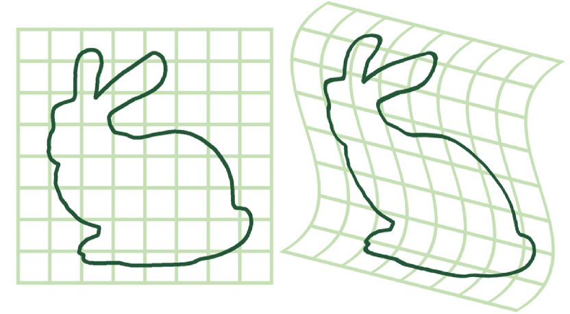
Figure 2: A 2D visualization of an object deforming with the cage.

The global matrix can be assembled using a pre-trained convolutional neural network (see appendix). However, its inverse still needs to be recomputed per timestep. To make it matrix-free, we use an iterative Jacobi method to solve the linear system. These methods converge faster for high-frequency components but require more iterations for low-frequency motion. To address this issue, we construct a low-frequency subspace to project the system into, resolving low-frequency components initially. Subsequently, a few iterations of Jacobi effectively resolve both low and high-frequency components. Determining the subspace involves performing an SVD on the global matrix per timestep. Since our objects are inside a large box, we use the box’s subspace as a general subspace, visualized as encasing the 3D model within a cage (Fig. 2). The object deforms and moves with the cage’s deformations and motions, with a few Jacobi iterations fine-tuning the high-frequency components.

Thanks to the discrete voxel format, each point during Jacobi iterations interacts only with its neighbors. Therefore, each Jacobi iteration is equivalent to collecting information from each point’s $1$-ring neighbors to update that point’s information. Following this idea, we train a CNN to implement this process. Moreover, inspired by Lan et al. [36], we can increase the kernel size of this CNN to collect information from $2$-ring neighbors in a iteration, thereby doubling the efficiency. Derivations and details can be found in the appendix.

5 Experiments

We implement our method using Python. In addition, we use PyTorch [28] to implement the network and simulator. Our hardware platform is a desktop computer equipped with an Intel i7-12700F CPU and an NVIDIA 3090 GPU. Detailed statistics of the settings, models, and fitting errors are reported in Tab. 1. All experiments are also available in the supplemental video.

Table 1: Experiments statistics. We report detailed settings of our experiments. $\#$DoFs: the average degree of freedoms in our optimization. $\Delta t$: the size of timestep. $\#$L-G: the average number of local-global iterations for each timestep. $\#$Jacobi: the average number of Jacobi iterations for each timestep. EM: the elastic model. Fitting error: the loss of neural metric in Eq. (9). $t/\text{frame}$: the seconds consumed per frame. The slash sign $/$ means several different settings.

Scene	Grid resolution	$\#$DoFs	$\Delta t$	$\#$L-G	$\#$Jacobi	EM	Fitting error	$t/\text{frame}$
ShapeNet(Fig. 3)	$32\times 32\times 32$	$5\text{K}$	$0.002$	$10$	$213$	NH	$1.32\times 10^{-4}$	$0.08$
Cantilever(Fig. 4)	$16\times 3\times 3$	$432$	$0.001$	$5$	$108$	$/$	$4.11\times 10^{-4}$	$0.01$
Cantilever(Fig. 7)	$16\times 3\times 3$	$432$	$0.001$	$15$	$/$	NH	$9.67\times 10^{-5}$	$0.01$
Lego(Fig. 5)	$26\times 46\times 30$	$11\text{K}$	$0.005$	$15$	$320$	NH	$2.34\times 10^{-4}$	$2.10$
Drums(Fig. 5)	$28\times 22\times 34$	$4\text{K}$	$0.005$	$15$	$320$	CR	$7.63\times 10^{-5}$	$0.21$
Bridge(Fig. 6)	$66\times 13\times 27$	$7\text{K}$	$0.003$	$5$	$96$	StVK	$5.78\times 10^{-4}$	$0.12$
Ship(Fig. 6)	$53\times 33\times 16$	$14\text{K}$	$0.001$	$5$	$100$	NH	$2.34\times 10^{-4}$	$1.20$

5.1 Experiments on ShapeNet dataset

To demonstrate the feasibility of our method across various shapes, we conduct experiments on multiple models from ShapeNet [10] with different force and pin settings (Fig. 3). As discussed, our network training relies on voxel-to-tetrahedral decomposition and the energy model, making ElastoGen theoretically capable of handling any shape. All models are divided into a $32\times 32\times 32$ voxel grid and use the same general subspace. Cabinets are pinned at the bottom, twisted, and then released to oscillate elastically. Towers and plants are pinned at the base and swayed by wind forces. Airplanes are pinned at the middle and nose with varying external forces, resulting in three distinct dynamic effects. The results confirm our hypothesis, showing that different boundary conditions and external forces produce plausible dynamic outcomes. More results are available in the appendix.

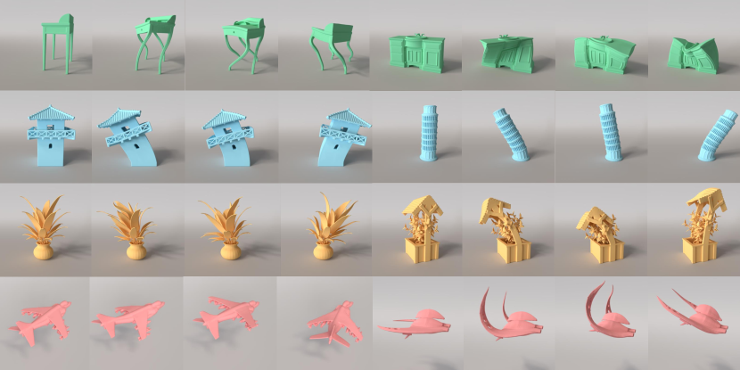
Figure 3: ShapeNet experiments. To demonstrate the feasibility of our method across various shapes, we pin different points and exert different external forces (e.g., gravity, drag, twist, force field) on four categories of the ShapeNet dataset, i.e. cabinets(green), towers(blue), plants(yellow), and airplanes(red). These experiments are run with a grid resolution size of $32\times 32\times 32$.

5.2 Validation on various elastic models

ElastoGen can handle various elastic materials and different material parameters. We validate the elastic response using the classic cantilever beam experiment. The experiment includes beams with three elastic materials: co-rotational [9], Neo-Hookean [67], and StVK [5]. More general nonlinear materials, such as spline-based materials [70], are also supported though not included here. Each material is tested with three different Poisson’s ratios while keeping a fixed Young’s modulus. The results, as shown in the Fig. 4(b), align with our expectations. Higher Poisson’s ratios result in stronger volume-preserving effects, while the stiffness varies from hard to soft in the order of StVK, Neo-Hookean, and co-rotational materials. We also visualize the total elastic energy over time for the three materials with a Poisson’s ratio of $0.2435$ (Fig. 4(c)), confirming that the visual results match our expectations. Additionally, we visualize the fitting of the network parameters (Fig. 4(a)), generated through diffusion, to energy models. To provide a clearer visualization, we display the elastic energy curves with respect to deformation gradient along $x$-axis. The visualizations demonstrate that our generated network parameters fit the elastic energy well.

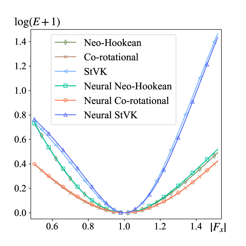
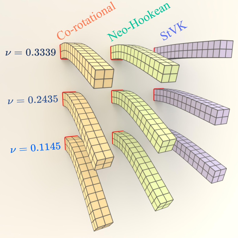
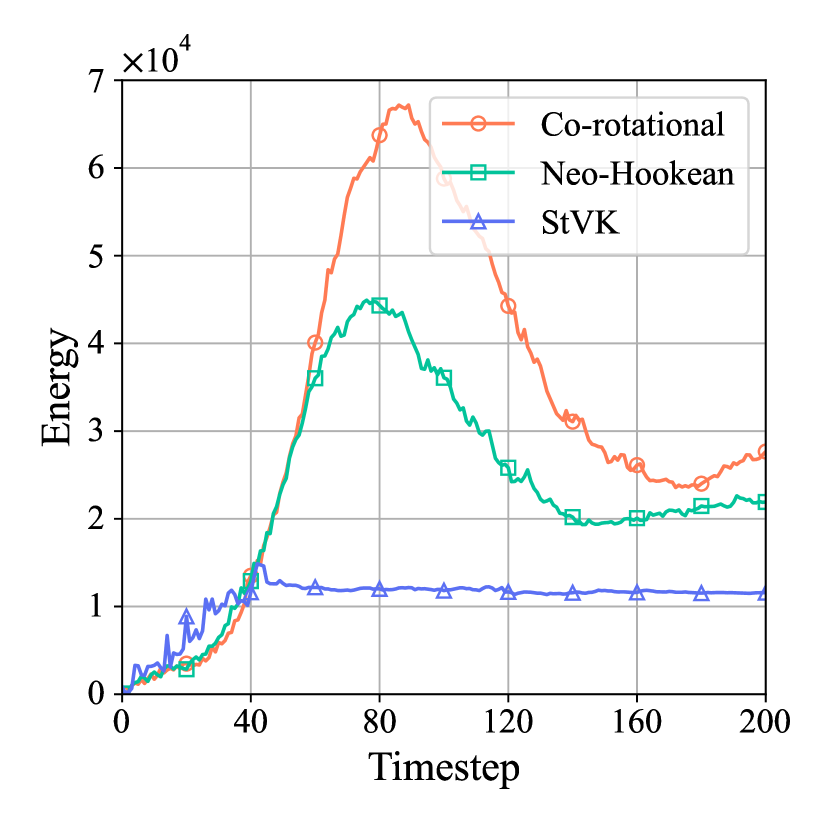
Figure 4: Comparison of different materials on cantilever beam. (a) 1D visualization of neural material fitting. (b) Comparison of material parameters. (c) Elastic energy vs. time for different materials with Poisson’s ratio fixed.

5.3 Versatility across geometric representations

Our method can be applied to any geometric representation. For instance, when using implicit Neural Radiance Fields (NeRF) [50] to describe 3D models, we employ the technique from PIE-NeRF [16]. First, we voxelize the NeRF based on the density fields. Then, we generate dynamics using ElastoGen and finally obtain a dynamic NeRF through linear ray warping [16]. As shown in Fig. 5, we test this pipeline on the standard NeRF dataset, generating dynamic NeRF.

Our method is also applicable to complex explicit meshes. We test our approach on meshes with intricate geometries, achieving similarly impressive results. With adaptive resolution for voxelization, ElastoGen produces visually pleasing and physically accurate dynamics while preserving the dynamic details of the fine structures. In Fig. 6, the deformation of each steel bar on the bridge is visible, as well as the bending and stretching of the sails and ropes on the ship’s masts.

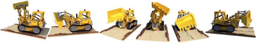
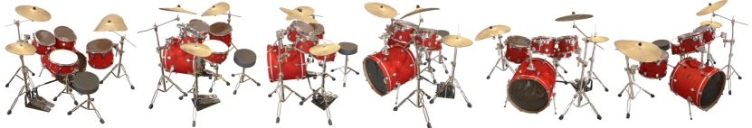
Figure 5: NeRF experiments. Our method is compatible with the NeRF dataset. We voxelize the NeRF based on density fields, generate dynamics using ElastoGen, and render through ray warping.

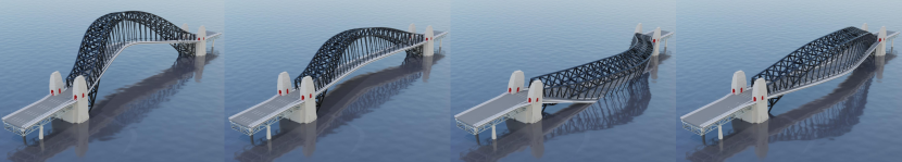
Figure 6: Experiments on complex scenes. ElastoGen effectively handles complex meshes with intricate geometries and fine structures. With adaptive spatial resolutions, ElastoGen preserves dynamic details such as the deformation of steel bars on the bridge and the bending of sails and ropes on the ship’s masts.

5.4 Comparison and ablation study

Compare with ground truth. We compare our method with the classic FEM simulator [61] due to its robustness, serving as the ground truth. We test a Neo-Hookean material by twisting and releasing a cantilever beam with gravity off to compare the dynamics between FEM and ElastoGen. We use a general subspace with 3 and 10 iterations of the Jacobi method. Fig. 7(a) shows that with 3 iterations, the results exhibit significant damping due to incomplete numerical convergence, resulting in very rigid dynamics. With 10 iterations, although differences from FEM remain, the damping is noticeably reduced, leading to much softer dynamics.

Ablation study on general subspace. To quantify the impact of Jacobi iterations and the general subspace on results, we compare different Jacobi iterations to a direct solver for matrix inversion in terms of relative error. A smaller error indicates greater displacement and softer dynamics. All methods perform 20 local-global iterations per timestep. Fig. 7(b) shows that 50 Jacobi iterations nearly match the direct solver, and 20 iterations yield satisfactory results. In contrast, 1, 3, and 5 iterations result in noticeably stiffer dynamics.

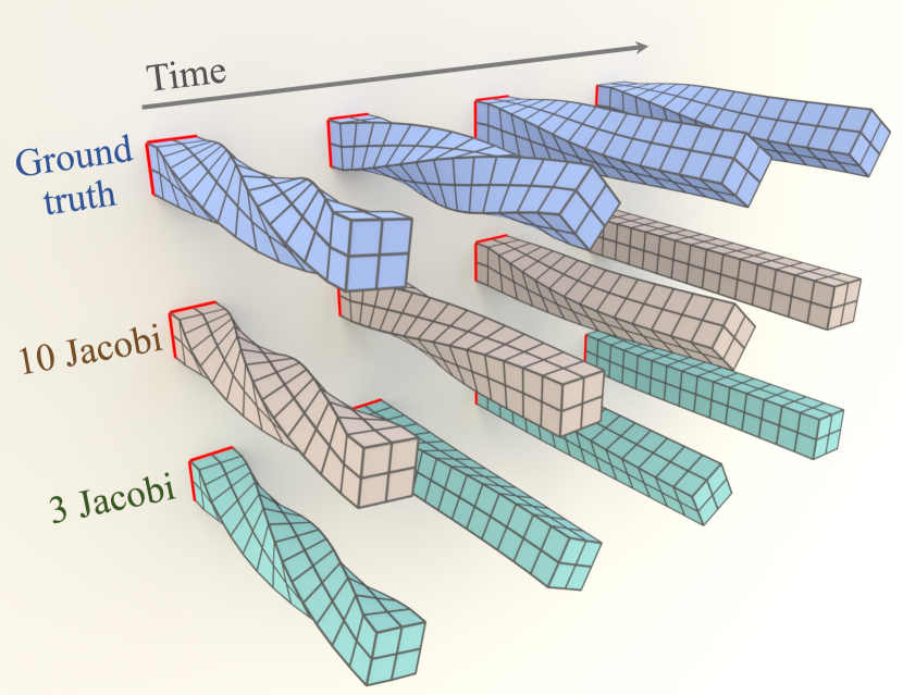
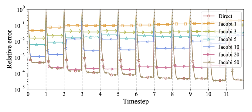
Figure 7: Validation of the use of general subspace with Jacobi iterations for global step. (a) Comparison to FEM using different Jacobi iterations on a twisted cantilever beam. (b) Relative errors for local-global iterations within each timestep.

6 Conclusion, Limitations, and Future Work

ElastoGen is an innovative framework that embeds physical laws and computational physics principles directly into network design, creating lightweight and compact networks with clear, specific functions for each module. This design allows for efficient, decoupled training, eliminating the need for large datasets, and excels in generating accurate physics-based dynamics, establishing a new benchmark for practical and effective solutions. However, it has limitations: it lacks support for collisions, is computationally inefficient due to convolution operations on empty voxels, and may fail to converge with extremely stiff materials due to the general subspace method, leading to unrealistic dynamics. Future work will address these issues by integrating dynamics for more materials (e.g., fluids, rigid bodies, and plasticity), adding collision support, and automating the setting of physical parameters and boundary conditions to ultimately achieve the goal of generating real-world dynamics.

Appendix A Appendix / supplemental material

A.1 Supplemental video

We refer the readers to the supplementary video to view the animated results for all examples.

A.2 Convolutional deformation gradient

To solve our nonlinear optimization problem, computing the deformation gradient is essential. The deformation gradient is the derivative of each component of the deformed vector $\mathbf{x}$ with respect to each component of the reference vector $\mathbf{X}$. For deformation map $\mathbf{x}=\mathbf{x}(\mathbf{X})$, we have:

$$\mathbf{F}=\frac{\partial\mathbf{x}}{\partial\mathbf{X}}.$$ (11)

In a tetrahedron, we can compute the deformation gradient using the following equation:

$$\begin{split}\mathbf{F}&=\mathbf{x}\mathbf{G},\end{split}$$ (12)

where script $i$ means the $i$-th point in the tetrahedron, and $\mathbf{G}$ is a discrete differential operator that corresponds to the rest configuration. In our implementation, we use a CNN with an input channel of $3$, an output channel of $54$ (corresponding to $6$ tetrahedra each with $9$ elements) and a kernel size of $2$ to learn this differential operator. We collect a dataset using traditional numerical methods and train the CNN to calculate the deformation gradient.

A.3 Global phase

As stated in the main text, we need to solve the linear system in Eq. (10), which requires determining $\mathbf{b}_{i}$ and $\mathbf{L}_{i}$. Due to our lagging operation, we abbreviate $\mathbf{N}(\mathbf{F}_{n})$ as $\mathbf{N}$, so $E_{i}$ becomes:

$$E_{i}=\frac{\omega_{i}}{2}\left\|\mathbf{F}_{i}\mathbf{N}_{i}-\mathbf{R}_{i}\right\|^{2},$$ (13)

where $\mathbf{R}_{i}$ is the rotation part of $\mathbf{F}_{i}$. Furthermore, based on $\mathbf{L}_{i}\mathbf{q}-\mathbf{b}_{i}:=\frac{\partial E_{i}}{\partial\mathbf{q}}$, we can obtain the expression for $\mathbf{b}_{i}$ and $\mathbf{L}_{i}$. If the four points of the tetrahedron form the matrix $\mathbf{x}_{i}$ as Eq.(12), then:

$$\frac{\partial E_{i}}{\partial\mathbf{x}_{i}}=\omega_{i}\left(\mathbf{x}_{i}\mathbf{G}_{i}\mathbf{N}_{i}\mathbf{N}_{i}^{\top}\mathbf{G}_{i}^{\top}-\mathbf{R}_{i}\mathbf{N}_{i}\mathbf{G}_{i}^{\top}\right).$$ (14)

Therefore, for each voxel, we can obtain $\mathbf{b_{i}}$ by applying the transpose transformation of $\mathbf{G}_{i}$ to $\mathbf{R}_{i}\mathbf{N}_{i}$. For $\mathbf{G}_{i}$ has been trained as a convolutional kernel as described in § A.2, we can directly use the previously trained kernel and perform the transposed convolution operation.

Using the Jacobi method to solve the linear system $\mathbf{A}\mathbf{x}=\mathbf{b}$ can be write as:

$$\mathbf{x}_{n+1}=\mathbf{D}^{-1}(\mathbf{b}-\mathbf{S}\mathbf{x}_{n}),$$ (15)

where $\mathbf{D}$ is the diagonal of $\mathbf{A}$ and $\mathbf{S}=\mathbf{A}-\mathbf{D}$. $\mathbf{x}_{n}$ is the result after $n$ iterations. If we use $\mathbf{x}_{n}$ to directly compute $\mathbf{x}_{n+2}$, we have

$$\mathbf{x}_{n+2}=\mathbf{D}^{-1}\mathbf{b}-\mathbf{D}^{-1}\mathbf{S}\mathbf{D}^{-1}\mathbf{b}+\mathbf{D}^{-1}\mathbf{S}\mathbf{D}^{-1}\mathbf{S}\mathbf{x}_{n}.$$ (16)

In our case, if we use the $1$-ring neighbor Jacobi method as in Eq. (15), we need to solve for $\mathbf{S}\mathbf{x}_{n}$, specifically the off-diagonal terms of $\mathbf{L}_{i}\mathbf{x}$. To achieve this, we fit a CNN that takes $\mathbf{N}_{i}$ and $\mathbf{x}_{n}$ as inputs and outputs $\mathbf{x}\mathbf{G}_{i}\mathbf{N}_{i}\mathbf{N}_{i}^{T}\mathbf{G}_{i}^{T}$. Each voxel has $8$ vertices, with each vertex having $3$ degrees of freedom, and each voxel has six $\mathbf{N}_{i}$. Therefore, the number of input channels is $78$, and the number of output channels is $24$, with a kernel size of $1$, representing the contribution of each voxel to its $8$ vertices. When using $2$-ring neighbors, we simply change the kernel size to $3$.

A.4 Datasets

To train the two small networks mentioned earlier, we need the corresponding datasets. For the network in § A.2, we randomly generate deformation gradients $\mathbf{F}$ for $B$ voxels and compute the corresponding $\mathbf{x}$ based on $\mathbf{F}$ and voxels’ tetrahedral topology. We need to fit a CNN with an input channel of $3$, an output channel of $54$, a kernel size of $2$, and a stride of $1$.

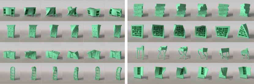
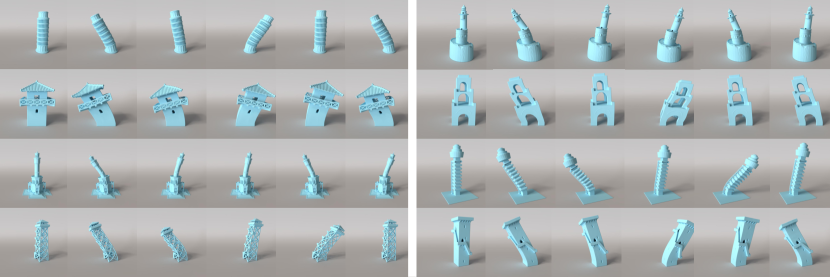
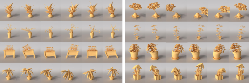
Figure 8: Additional experiments on ShapeNet. Here are more results of cabinets, towers, and plants.

To ensure our network can handle all deformation scenarios, we sample $\mathbf{F}$ using the following strategy: we randomly sample $3\times 6\times B$ numbers $\{l\}_{3\times 6\times B}$, each from a normal distribution $\mathcal{N}(0,1.5)$. These numbers represent the stretching of $B\times 6$ tetrahedra along three directions. To ensure that compression and stretching are equally represented in the data, for each positive $l$, we set $l^{\prime}=l+1$; for each negative $l$, we set $l^{\prime}=0.99e^{l}+0.01$. We then apply random rotations to combine with the stretching to obtain $\mathbf{F}$. Subsequently, we derive the coordinates $\mathbf{x}$ of each voxel’s vertices from $\mathbf{F}$. The pairs $\{\mathbf{x},\mathbf{F}\}$ form our dataset.

For the network in § A.3, we generate $B\times 6$ random matrices $\mathbf{M}$ and use $\mathbf{N}=\mathbf{M}+\mathbf{M}^{\top}$ along with $\mathbf{x}$ computed in the previous paragraph as the input. The $2$-ring neighbor Jacobi computed using Eq. (14) and Eq. (16) serves as the ground truth output. For both networks, we use Mean Squared Error (MSE) as the loss metric.

A.5 Broader impact

Our model integrates computational physics knowledge into the network structure design, significantly reducing the data requirements and making both the training and network structure more lightweight. It blends the boundaries among machine learning, graphics, and computational physics, providing new perspectives for network design. Our model does not necessarily bring about any significant ethical considerations.

A.6 More experiments

We provide additional results in Fig. 8 and Fig. 9 to demonstrate the robustness of ElastoGen. For more animated results, we refer the readers to supplemental video.

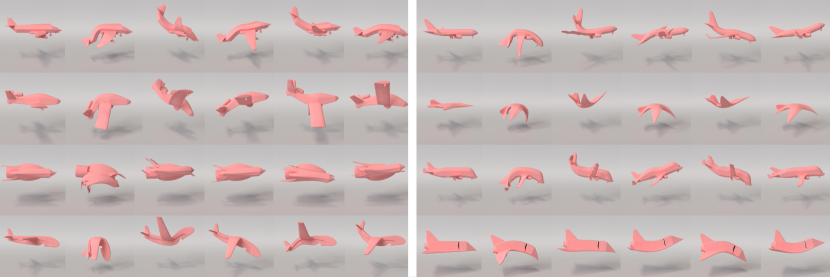
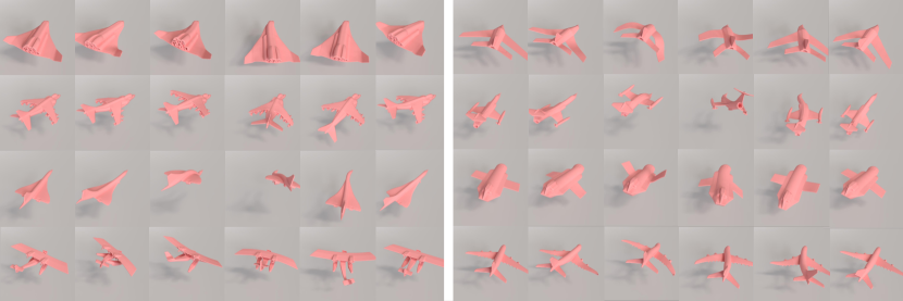
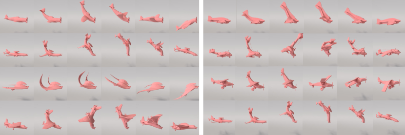
Figure 9: Additional experiments on ShapeNet (continued). Here are more results of airplanes with different force and boundary settings.

References

- Ajay et al. [2018] Anurag Ajay, Jiajun Wu, Nima Fazeli, Maria Bauza, Leslie P Kaelbling, Joshua B Tenenbaum, and Alberto Rodriguez. Augmenting physical simulators with stochastic neural networks: Case study of planar pushing and bouncing. In 2018 IEEE/RSJ International Conference on Intelligent Robots and Systems (IROS), pages 3066–3073. IEEE, 2018.
- Arjovsky et al. [2017] Martin Arjovsky, Soumith Chintala, and Léon Bottou. Wasserstein gan, 2017.
- Bahmani et al. [2024a] Sherwin Bahmani, Xian Liu, Yifan Wang, Ivan Skorokhodov, Victor Rong, Ziwei Liu, Xihui Liu, Jeong Joon Park, Sergey Tulyakov, Gordon Wetzstein, et al. Tc4d: Trajectory-conditioned text-to-4d generation. arXiv preprint arXiv:2403.17920, 2024a.
- Bahmani et al. [2024b] Sherwin Bahmani, Ivan Skorokhodov, Victor Rong, Gordon Wetzstein, Leonidas Guibas, Peter Wonka, Sergey Tulyakov, Jeong Joon Park, Andrea Tagliasacchi, and David B. Lindell. 4d-fy: Text-to-4d generation using hybrid score distillation sampling. IEEE Conference on Computer Vision and Pattern Recognition (CVPR), 2024b.
- Barbič and James [2005] Jernej Barbič and Doug L James. Real-time subspace integration for st. venant-kirchhoff deformable models. ACM transactions on graphics (TOG), 24(3):982–990, 2005.
- Battaglia et al. [2016] Peter Battaglia, Razvan Pascanu, Matthew Lai, Danilo Jimenez Rezende, et al. Interaction networks for learning about objects, relations and physics. Advances in neural information processing systems, 29, 2016.
- Blattmann et al. [2023] Andreas Blattmann, Robin Rombach, Huan Ling, Tim Dockhorn, Seung Wook Kim, Sanja Fidler, and Karsten Kreis. Align your latents: High-resolution video synthesis with latent diffusion models, 2023.
- Bouaziz et al. [2014] Sofien Bouaziz, Sebastian Martin, Tiantian Liu, Ladislav Kavan, and Mark Pauly. Projective dynamics: fusing constraint projections for fast simulation. ACM Trans. Graph., 33(4), 2014.
- Brogan [1986] FA Brogan. An element independent corotational procedure for the treatment of large rotations. Journal of Pressure Vessel Technology, 108:165, 1986.
- Chang et al. [2015] Angel X Chang, Thomas Funkhouser, Leonidas Guibas, Pat Hanrahan, Qixing Huang, Zimo Li, Silvio Savarese, Manolis Savva, Shuran Song, Hao Su, et al. Shapenet: An information-rich 3d model repository. arXiv preprint arXiv:1512.03012, 2015.
- Chang et al. [2017] Michael Chang, Tomer D. Ullman, Antonio Torralba, and Joshua B. Tenenbaum. A compositional object-based approach to learning physical dynamics. In 5th International Conference on Learning Representations, ICLR 2017, Toulon, France, April 24-26, 2017, Conference Track Proceedings. OpenReview.net, 2017.
- Child [2021] Rewon Child. Very deep vaes generalize autoregressive models and can outperform them on images. In 9th International Conference on Learning Representations, ICLR 2021, Virtual Event, Austria, May 3-7, 2021. OpenReview.net, 2021.
- Chu et al. [2022] Mengyu Chu, Lingjie Liu, Quan Zheng, Erik Franz, Hans-Peter Seidel, Christian Theobalt, and Rhaleb Zayer. Physics informed neural fields for smoke reconstruction with sparse data. ACM Trans. Graph., 41(4), 2022.
- Dinh et al. [2015] Laurent Dinh, David Krueger, and Yoshua Bengio. Nice: Non-linear independent components estimation, 2015.
- Dinh et al. [2017] Laurent Dinh, Jascha Sohl-Dickstein, and Samy Bengio. Density estimation using real NVP. In 5th International Conference on Learning Representations, ICLR 2017, Toulon, France, April 24-26, 2017, Conference Track Proceedings. OpenReview.net, 2017.
- Feng et al. [2023] Yutao Feng, Yintong Shang, Xuan Li, Tianjia Shao, Chenfanfu Jiang, and Yin Yang. Pie-nerf: Physics-based interactive elastodynamics with nerf. arXiv preprint arXiv:2311.13099, 2023.
- Feng et al. [2024] Yutao Feng, Xiang Feng, Yintong Shang, Ying Jiang, Chang Yu, Zeshun Zong, Tianjia Shao, Hongzhi Wu, Kun Zhou, Chenfanfu Jiang, et al. Gaussian splashing: Dynamic fluid synthesis with gaussian splatting. arXiv preprint arXiv:2401.15318, 2024.
- Geng et al. [2020] Zhenglin Geng, Daniel Johnson, and Ronald Fedkiw. Coercing machine learning to output physically accurate results. J. Comput. Phys., 406:109099, 2020.
- Gibou et al. [2019] Frederic Gibou, David Hyde, and Ron Fedkiw. Sharp interface approaches and deep learning techniques for multiphase flows. Journal of Computational Physics, 380:442–463, 2019.
- Godunov and Bohachevsky [1959] Sergei K Godunov and I Bohachevsky. Finite difference method for numerical computation of discontinuous solutions of the equations of fluid dynamics. Matematičeskij sbornik, 47(3):271–306, 1959.
- Goodfellow et al. [2014] Ian Goodfellow, Jean Pouget-Abadie, Mehdi Mirza, Bing Xu, David Warde-Farley, Sherjil Ozair, Aaron Courville, and Yoshua Bengio. Generative adversarial nets. Advances in neural information processing systems, 27, 2014.
- Gulrajani et al. [2017] Ishaan Gulrajani, Faruk Ahmed, Martín Arjovsky, Vincent Dumoulin, and Aaron C. Courville. Improved training of wasserstein gans. In Advances in Neural Information Processing Systems 30: Annual Conference on Neural Information Processing Systems 2017, December 4-9, 2017, Long Beach, CA, USA, pages 5767–5777, 2017.
- Harvey et al. [2022] William Harvey, Saeid Naderiparizi, Vaden Masrani, Christian Weilbach, and Frank Wood. Flexible diffusion modeling of long videos. Advances in Neural Information Processing Systems, 35:27953–27965, 2022.
- Ho et al. [2020] Jonathan Ho, Ajay Jain, and Pieter Abbeel. Denoising diffusion probabilistic models. In Advances in Neural Information Processing Systems 33: Annual Conference on Neural Information Processing Systems 2020, NeurIPS 2020, December 6-12, 2020, virtual, 2020.
- Ho et al. [2022a] Jonathan Ho, William Chan, Chitwan Saharia, Jay Whang, Ruiqi Gao, Alexey Gritsenko, Diederik P Kingma, Ben Poole, Mohammad Norouzi, David J Fleet, et al. Imagen video: High definition video generation with diffusion models. arXiv preprint arXiv:2210.02303, 2022a.
- Ho et al. [2022b] Jonathan Ho, Tim Salimans, Alexey Gritsenko, William Chan, Mohammad Norouzi, and David J Fleet. Video diffusion models. Advances in Neural Information Processing Systems, 35:8633–8646, 2022b.
- Huebner et al. [2001] Kenneth H Huebner, Donald L Dewhirst, Douglas E Smith, and Ted G Byrom. The finite element method for engineers. John Wiley & Sons, 2001.
- Imambi et al. [2021] Sagar Imambi, Kolla Bhanu Prakash, and GR Kanagachidambaresan. Pytorch. Programming with TensorFlow: Solution for Edge Computing Applications, pages 87–104, 2021.
- Jain et al. [2022] Ajay Jain, Ben Mildenhall, Jonathan T Barron, Pieter Abbeel, and Ben Poole. Zero-shot text-guided object generation with dream fields. In Proceedings of the IEEE/CVF conference on computer vision and pattern recognition, pages 867–876, 2022.
- Jiang et al. [2024] Ying Jiang, Chang Yu, Tianyi Xie, Xuan Li, Yutao Feng, Huamin Wang, Minchen Li, Henry Lau, Feng Gao, Yin Yang, et al. Vr-gs: A physical dynamics-aware interactive gaussian splatting system in virtual reality. arXiv preprint arXiv:2401.16663, 2024.
- Karras et al. [2023] Johanna Karras, Aleksander Holynski, Ting-Chun Wang, and Ira Kemelmacher-Shlizerman. Dreampose: Fashion image-to-video synthesis via stable diffusion. In 2023 IEEE/CVF International Conference on Computer Vision (ICCV), pages 22623–22633. IEEE, 2023.
- Kerbl et al. [2023] Bernhard Kerbl, Georgios Kopanas, Thomas Leimkühler, and George Drettakis. 3d gaussian splatting for real-time radiance field rendering. ACM Transactions on Graphics, 42(4), 2023.
- Kingma and Dhariwal [2018] Diederik P. Kingma and Prafulla Dhariwal. Glow: Generative flow with invertible 1x1 convolutions. In Advances in Neural Information Processing Systems 31: Annual Conference on Neural Information Processing Systems 2018, NeurIPS 2018, December 3-8, 2018, Montréal, Canada, pages 10236–10245, 2018.
- Kingma and Welling [2014] Diederik P Kingma and Max Welling. Auto-encoding variational Bayes. In International Conference on Learning Representations (ICLR), 2014.
- Kipf et al. [2018] Thomas Kipf, Ethan Fetaya, Kuan-Chieh Wang, Max Welling, and Richard Zemel. Neural relational inference for interacting systems. In International conference on machine learning, pages 2688–2697. PMLR, 2018.
- Lan et al. [2022] Lei Lan, Guanqun Ma, Yin Yang, Changxi Zheng, Minchen Li, and Chenfanfu Jiang. Penetration-free projective dynamics on the gpu. 2022.
- Li et al. [2023] Xuan Li, Yi-Ling Qiao, Peter Yichen Chen, Krishna Murthy Jatavallabhula, Ming C. Lin, Chenfanfu Jiang, and Chuang Gan. Pac-nerf: Physics augmented continuum neural radiance fields for geometry-agnostic system identification. In The Eleventh International Conference on Learning Representations, ICLR 2023, Kigali, Rwanda, May 1-5, 2023. OpenReview.net, 2023.
- Li et al. [2019a] Yunzhu Li, Hao He, Jiajun Wu, Dina Katabi, and Antonio Torralba. Learning compositional koopman operators for model-based control. arXiv preprint arXiv:1910.08264, 2019a.
- Li et al. [2019b] Yunzhu Li, Jiajun Wu, Russ Tedrake, Joshua B. Tenenbaum, and Antonio Torralba. Learning particle dynamics for manipulating rigid bodies, deformable objects, and fluids. In 7th International Conference on Learning Representations, ICLR 2019, New Orleans, LA, USA, May 6-9, 2019. OpenReview.net, 2019b.
- Li et al. [2019c] Yunzhu Li, Jiajun Wu, Jun-Yan Zhu, Joshua B Tenenbaum, Antonio Torralba, and Russ Tedrake. Propagation networks for model-based control under partial observation. In 2019 International Conference on Robotics and Automation (ICRA), pages 1205–1211. IEEE, 2019c.
- Lin et al. [2023] Chen-Hsuan Lin, Jun Gao, Luming Tang, Towaki Takikawa, Xiaohui Zeng, Xun Huang, Karsten Kreis, Sanja Fidler, Ming-Yu Liu, and Tsung-Yi Lin. Magic3d: High-resolution text-to-3d content creation. In Proceedings of the IEEE/CVF Conference on Computer Vision and Pattern Recognition, pages 300–309, 2023.
- Ling et al. [2023] Huan Ling, Seung Wook Kim, Antonio Torralba, Sanja Fidler, and Karsten Kreis. Align your gaussians: Text-to-4d with dynamic 3d gaussians and composed diffusion models. arXiv preprint arXiv:2312.13763, 2023.
- Liu et al. [2024] Minghua Liu, Chao Xu, Haian Jin, Linghao Chen, Mukund Varma T, Zexiang Xu, and Hao Su. One-2-3-45: Any single image to 3d mesh in 45 seconds without per-shape optimization. Advances in Neural Information Processing Systems, 36, 2024.
- Liu et al. [2023] Ruoshi Liu, Rundi Wu, Basile Van Hoorick, Pavel Tokmakov, Sergey Zakharov, and Carl Vondrick. Zero-1-to-3: Zero-shot one image to 3d object. In Proceedings of the IEEE/CVF International Conference on Computer Vision, pages 9298–9309, 2023.
- Liu et al. [2013] Tiantian Liu, Adam W Bargteil, James F O’Brien, and Ladislav Kavan. Fast simulation of mass-spring systems. ACM Transactions on Graphics (TOG), 32(6):1–7, 2013.
- Liu et al. [2017] Tiantian Liu, Sofien Bouaziz, and Ladislav Kavan. Quasi-newton methods for real-time simulation of hyperelastic materials. ACM Transactions on Graphics (TOG), 36(3):23, 2017.
- Mescheder [2018] Lars M. Mescheder. On the convergence properties of GAN training. CoRR, abs/1801.04406, 2018.
- Metzer et al. [2023] Gal Metzer, Elad Richardson, Or Patashnik, Raja Giryes, and Daniel Cohen-Or. Latent-nerf for shape-guided generation of 3d shapes and textures. In Proceedings of the IEEE/CVF Conference on Computer Vision and Pattern Recognition, pages 12663–12673, 2023.
- Mildenhall et al. [2020] Ben Mildenhall, Pratul P. Srinivasan, Matthew Tancik, Jonathan T. Barron, Ravi Ramamoorthi, and Ren Ng. Nerf: Representing scenes as neural radiance fields for view synthesis. In ECCV, 2020.
- Mildenhall et al. [2021] Ben Mildenhall, Pratul P Srinivasan, Matthew Tancik, Jonathan T Barron, Ravi Ramamoorthi, and Ren Ng. Nerf: Representing scenes as neural radiance fields for view synthesis. Communications of the ACM, 65(1):99–106, 2021.
- Müller et al. [2007] Matthias Müller, Bruno Heidelberger, Marcus Hennix, and John Ratcliff. Position based dynamics. Journal of Visual Communication and Image Representation, 18(2):109–118, 2007.
- Murray [1997] Richard M Murray. Nonlinear control of mechanical systems: A lagrangian perspective. Annual Reviews in Control, 21:31–42, 1997.
- Ni et al. [2023] Haomiao Ni, Changhao Shi, Kai Li, Sharon X Huang, and Martin Renqiang Min. Conditional image-to-video generation with latent flow diffusion models. In Proceedings of the IEEE/CVF Conference on Computer Vision and Pattern Recognition, pages 18444–18455, 2023.
- Pakravan et al. [2021] Samira Pakravan, Pouria A Mistani, Miguel A Aragon-Calvo, and Frederic Gibou. Solving inverse-pde problems with physics-aware neural networks. Journal of Computational Physics, 440:110414, 2021.
- Poole et al. [2022] Ben Poole, Ajay Jain, Jonathan T Barron, and Ben Mildenhall. Dreamfusion: Text-to-3d using 2d diffusion. In The Eleventh International Conference on Learning Representations, 2022.
- Raissi et al. [2019] Maziar Raissi, Paris Perdikaris, and George E Karniadakis. Physics-informed neural networks: A deep learning framework for solving forward and inverse problems involving nonlinear partial differential equations. Journal of Computational physics, 378:686–707, 2019.
- Reddy [1993] Junuthula Narasimha Reddy. An introduction to the finite element method. New York, 27:14, 1993.
- Rombach et al. [2022] Robin Rombach, Andreas Blattmann, Dominik Lorenz, Patrick Esser, and Björn Ommer. High-resolution image synthesis with latent diffusion models. In Proceedings of the IEEE/CVF conference on computer vision and pattern recognition, pages 10684–10695, 2022.
- Sanchez-Gonzalez et al. [2018] Alvaro Sanchez-Gonzalez, Nicolas Heess, Jost Tobias Springenberg, Josh Merel, Martin Riedmiller, Raia Hadsell, and Peter Battaglia. Graph networks as learnable physics engines for inference and control. In International conference on machine learning, pages 4470–4479. PMLR, 2018.
- Shen et al. [2023] Liao Shen, Xingyi Li, Huiqiang Sun, Juewen Peng, Ke Xian, Zhiguo Cao, and Guosheng Lin. Make-it-4d: Synthesizing a consistent long-term dynamic scene video from a single image. In Proceedings of the 31st ACM International Conference on Multimedia, pages 8167–8175, 2023.
- Sifakis and Barbic [2012] Eftychios Sifakis and Jernej Barbic. Fem simulation of 3d deformable solids: a practitioner’s guide to theory, discretization and model reduction. In Acm siggraph 2012 courses, pages 1–50. 2012.
- Singer et al. [2023] Uriel Singer, Shelly Sheynin, Adam Polyak, Oron Ashual, Iurii Makarov, Filippos Kokkinos, Naman Goyal, Andrea Vedaldi, Devi Parikh, Justin Johnson, et al. Text-to-4d dynamic scene generation. arXiv preprint arXiv:2301.11280, 2023.
- Sohl-Dickstein et al. [2015] Jascha Sohl-Dickstein, Eric A. Weiss, Niru Maheswaranathan, and Surya Ganguli. Deep unsupervised learning using nonequilibrium thermodynamics. In Proceedings of the 32nd International Conference on Machine Learning, ICML 2015, Lille, France, 6-11 July 2015, pages 2256–2265. JMLR.org, 2015.
- Um et al. [2020] Kiwon Um, Robert Brand, Yun Raymond Fei, Philipp Holl, and Nils Thuerey. Solver-in-the-loop: Learning from differentiable physics to interact with iterative pde-solvers. Advances in Neural Information Processing Systems, 33:6111–6122, 2020.
- Vahdat and Kautz [2020] Arash Vahdat and Jan Kautz. NVAE: A deep hierarchical variational autoencoder. In Advances in Neural Information Processing Systems 33: Annual Conference on Neural Information Processing Systems 2020, NeurIPS 2020, December 6-12, 2020, virtual, 2020.
- Wang et al. [2024] Zhengyi Wang, Cheng Lu, Yikai Wang, Fan Bao, Chongxuan Li, Hang Su, and Jun Zhu. Prolificdreamer: High-fidelity and diverse text-to-3d generation with variational score distillation. Advances in Neural Information Processing Systems, 36, 2024.
- Wu et al. [2001] Xunlei Wu, Michael S Downes, Tolga Goktekin, and Frank Tendick. Adaptive nonlinear finite elements for deformable body simulation using dynamic progressive meshes. In Computer Graphics Forum, pages 349–358. Wiley Online Library, 2001.
- Xie et al. [2023] Tianyi Xie, Zeshun Zong, Yuxin Qiu, Xuan Li, Yutao Feng, Yin Yang, and Chenfanfu Jiang. Physgaussian: Physics-integrated 3d gaussians for generative dynamics. arXiv preprint arXiv:2311.12198, 2023.
- Xu et al. [2024] Dejia Xu, Hanwen Liang, Neel P Bhatt, Hezhen Hu, Hanxue Liang, Konstantinos N Plataniotis, and Zhangyang Wang. Comp4d: Llm-guided compositional 4d scene generation. arXiv preprint arXiv:2403.16993, 2024.
- Xu et al. [2015] Hongyi Xu, Funshing Sin, Yufeng Zhu, and Jernej Barbič. Nonlinear material design using principal stretches. ACM Transactions on Graphics (TOG), 34(4):1–11, 2015.
- Yang et al. [2020] Shuqi Yang, Xingzhe He, and Bo Zhu. Learning physical constraints with neural projections. Advances in Neural Information Processing Systems, 33:5178–5189, 2020.
- Yin et al. [2023] Yuyang Yin, Dejia Xu, Zhangyang Wang, Yao Zhao, and Yunchao Wei. 4dgen: Grounded 4d content generation with spatial-temporal consistency. arXiv preprint arXiv:2312.17225, 2023.
- Zhang et al. [2024] Baoquan Zhang, Chuyao Luo, Demin Yu, Xutao Li, Huiwei Lin, Yunming Ye, and Bowen Zhang. Metadiff: Meta-learning with conditional diffusion for few-shot learning. In Proceedings of the AAAI Conference on Artificial Intelligence, pages 16687–16695, 2024.
- Zhu et al. [2010] Yongning Zhu, Eftychios Sifakis, Joseph Teran, and Achi Brandt. An efficient multigrid method for the simulation of high-resolution elastic solids. ACM Trans. Graph., 29(2), 2010.
- Zienkiewicz and Morice [1971] Olgierd Cecil Zienkiewicz and PB Morice. The finite element method in engineering science. McGraw-hill London, 1971.
- Zienkiewicz et al. [2005] Olek C Zienkiewicz, Robert L Taylor, and Jian Z Zhu. The finite element method: its basis and fundamentals. Elsevier, 2005.