CCBNet: Confidential Collaborative Bayesian Networks Inference

Abstract

Effective large-scale process optimization in manufacturing industries requires close cooperation between different human expert parties who encode their knowledge of related domains as Bayesian network models. For instance, Bayesian networks for domains such as lithography equipment, processes, and auxiliary tools must be conjointly used to effectively identify process optimizations in the semiconductor industry. However, business confidentiality across domains hinders such collaboration, and encourages alternatives to centralized inference. We propose CCBNet, the first Confidentiality-preserving Collaborative Bayesian Network inference framework. CCBNet leverages secret sharing to securely perform analysis on the combined knowledge of party models by joining two novel subprotocols: (i) CABN, which augments probability distributions for features across parties by modeling them into secret shares of their normalized combination; and (ii) SAVE, which aggregates party inference result shares through distributed variable elimination. We extensively evaluate CCBNet via 9 public Bayesian networks. Our results show that CCBNet achieves predictive quality that is similar to the ones of centralized methods while preserving model confidentiality. We further demonstrate that CCBNet scales to challenging manufacturing use cases that involve 16–128 parties in large networks of 223–1003 features, and decreases, on average, computational overhead by 23%, while communicating 71k values per request. Finally, we showcase possible attacks and mitigations for partially reconstructing party networks in the two subprotocols.

1 Introduction

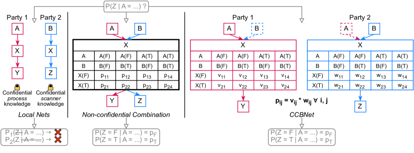
Figure 1: Sample Bayesian networks collaboration in semiconductor manufacturing: Parties’ separate models overlap within feature $X$. Party 1 features $A$ and $Y$ inform about the etching process and minimum feature size. Party 2 features $B$ and $Z$ inform about the wafer table and scanner overlay characteristics. After observing $A$, inferring updated state probabilities for $Z$ requires propagating information between $A$, $B$, and $X$, which is impossible by merely averaging model outputs. The typical non-confidential approach reveals the combined graph and probability tables to parties. CCBNet exchanges minimal structural information amongst parties, and secret shares overlap feature tables, reconstructing the final result by distributed inference.

Improving productivity and quality standards in manufacturing demands effectively expressing complex interactions between domain items. Bayesian networks (BNs) are commonly adopted to graphically model causality in manufacturing [22], with nodes representing features and directed edges showing dependencies. An essential trait of these models is their ability to specify arbitrary input and output features for each query instead of having them fixed.

Let us consider the use case of semiconductor manufacturing. Pursuing ever smaller size chips at a high yield [31] entails cooperation between many specialized parties that must protect their trade secrets. More specifically, fab operators encode their insight into settings dictating the production process in a BN. Similarly, vendors of equipment like scanners, construct BNs that describe the inner workings of their machines. Figure 1 illustrates such a scenario. Pooling together parties’ knowledge allows higher-quality analysis that optimize production environments, leading to new business opportunities. Simultaneously, the need to protect intellectual property expressed within party models calls for confidential collaboration.

Existing studies on collaborative inference for BNs disregard model confidentiality constraints or make concessions about which party information can be merged and how. Many have focused on centralized scenarios that combine local BNs’ knowledge into a larger one [11, 12] without protecting confidential knowledge within the input networks and global output. Models get stitched together based on common nodes, and remain in the final representation as largely unaltered sub-models whose encoded knowledge is easily inspectable. Pavlin et al. [24] proposes a distributed combination variant that partially preserves confidentiality by maintaining the locality of combined party models. However, it leaks information between parties when connecting them and does not allow merging inner graph nodes having both parents and children. Tedesco et al. [29] maintains the confidentiality of how nodes are linked within parties but only allows propagating information between them in a fixed sequential order. [19] is another distributed approach with similar confidentiality properties but even greater compatibility restrictions by requiring models to have identical inputs and outputs.

In this paper, we propose CCBNet, the first confidential, collaborative BNs inference framework that combines knowledge of multiple parties involved in inference queries through a novel secret sharing scheme. CCBNet does not require a trusted third party, and protects confidentiality at both the levels of party models and data instances. The two key components of CCBNet are: (i) confidential sharing of a normalized combination of features’ probability distributions across all overlapping parties; and (ii) distributed inference based on variable elimination for aggregating party results. The novelty of the augmentation procedure lies in constructing discrete conditional probability distributions for all features present in more than one party. These features represent secret shares of a combined and normalized distribution from a centralized scenario without exposing any party’s initial probability function. To evaluate CCBNet, we simulate knowledge compartmentalization over different starting public BNs. Moreover, we demonstrate possible attacks against the framework, their limitations, and ways to protect against them.

In summary, we make the following contributions:

• We devise a confidential, collaborative framework for BNs, CCBNet, that satisfies the needs of industry use cases like process optimization in manufacturing.

• We design a novel secret sharing-based protocol, CABN, to confidentially augment the conditional probability function of overlapping features in parties.

• We define SAVE, a new method for performing distributed inference on augmented party models backed by variable elimination that aggregates their result shares.

• We evaluate CCBNet over various scenarios based on nine public BNs. Our results indicate that CCBNet’s predictive accuracy is similar to those of non-confidential centralized alternatives and, for many collaborators in large networks, that CCBNet decreases the computational overhead by 23% on average when 71k values are communicated per request.

• We discuss attacks on the two CCBNet subprotocols, possible mitigation strategies and their trade-offs.

2 Background & Related Studies

2.1 Background

We review relevant BN notion with Figure 1 as reference.

Bayesian Networks are probabilistic graphical models that maintain explicit conditional probability distributions (CPDs) for features whose dependencies form a directed acyclic graph [28]. Within such context, features are often referred to as (probabilistic) variables or (graph) nodes. Shown in Figure 1, features and the influences between them give the graph nodes and edges, respectively. Principally for performance and interpretability, features in practical applications are generally discrete, with CPDs specifically embodying conditional probability tables. Learning may be driven by data, human experts, or both [20, 9], as with other human-readable models like decision trees. Automated learning discovers the graph structure and then populates CPD parameters from training data. Manual learning is desirable when incorporating concepts with known governing rules that need no approximation from observations. Examples are physical phenomena or, in manufacturing, human-engineered processes and tools, like Party 2’s scanner wafer table from Figure 1.

Inference in BNs finds updated posterior probabilities for the states of target variables, given the observed states of any evidence variables [26, 25]. As general inference is NP-Hard, approximate algorithms help decrease computation costs compared to exact ones while sacrificing some precision in the result. The main exact inference techniques are variable elimination and junction tree belief propagation, which decomposes the network into a tree of variable clusters, running variable elimination within them and then disseminating updates between neighbors by message-passing [20]. In Figure 1’s query, $Z$ is the target, given some observed state of $A$.

Computation in discrete BNs relies on a few base operations for propagating information: normalization, reduction, marginalization, and products [20]. We outline them with help from the non-confidential combination in Figure 1. Normalizing a CPD divides its entries by their column sum. Thus column summations, like $p_{11}+p_{21}$, would equal $1$. Reduction and marginalization remove variables from a CPD by fixing their states or, respectively, summing them out. Reducing or marginalizing $A$ from $X$ leaves $B$ as its sole parent. Flattening CPD structures yields factors that specify a value for each state combination of their variables without discriminating between the child and parents. Previous operations apply to both representations. Products operate on CPDs of the same variable or factors and create a new CPD/factor over the input variables’ union, where each entry is the multiplication of the corresponding ones in the original representations. The product of $X$ and $Z$’s factors, thus, additionally contains $A$ and $B$.

Markov random fields (MRFs) are a sibbling model of BNs, backed by undirected graphs, into which every BN is easily transformable via moralization [21, 27]. Apart from lacking acyclicity constraints, MRFs directly define parameters as factors and can deal with scenarios where edge directionality is unspecified, but BNs are more compact and efficient for generative use. For inference, BN properties and algorithms remain applicable. Thus, when aciclicity constraints are unsatisfiable, MRFs can still perform probabilistic inference like in BNs.

2.2 Prior Art

We identify two high-level categories of collaborative analysis for BNs: single- and multi-model. The first creates one global model, while the other keeps local models separate, merging their results.

Single-model approaches harness party data instances or models but neglect confidentiality. Federated learning discovers models [23, 13, 16, 1, 30] from private party instances with a coordinator, but fully decentralized alternatives exist [5, 14]. Direct network combination fuses structure [11, 2] and parameters [12] from party models.

Multi-model methods have parties work together during inference to produce a complete analysis result. Tedesco et al. [29] chains model without exchanging their contents but only allows using them one at a time in a predetermined order. Less confidential but more flexible, Pavlin et al. [24] fuses party networks based on common nodes but still requires them to be roots or leaves in the party’s directed acyclic graph. Ypma et al. [32] patents a collaborative solution for industrial processes, only mentioning data confidentiality preservation by anonymization. Kim and Ghahramani [19] runs models autonomously and only averages their final outputs, maintaining confidentiality but expecting models to share inputs and outputs.

In summary, single-model techniques break confidentiality by centralizing knowledge, and multi-model ones trade modeling power for it. CCBNet addresses both concerns.

3 CCBNet

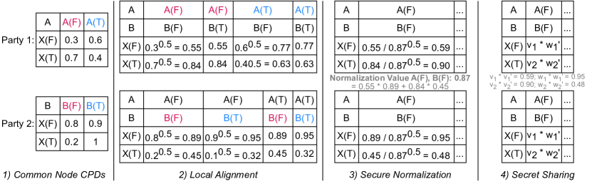
((a)) Key Steps of computing augmented CPDs

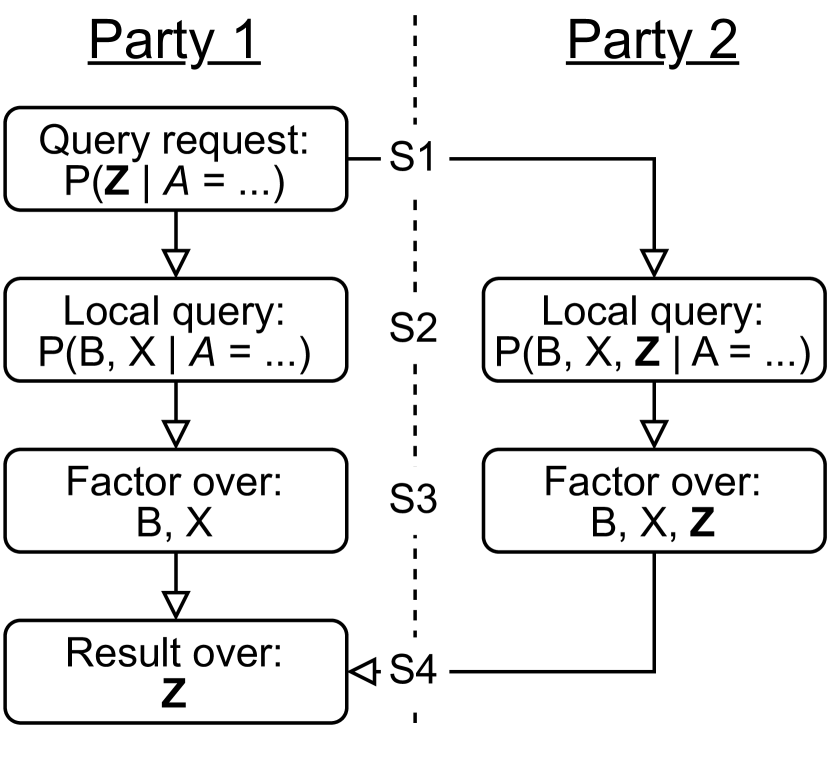
((b)) Distributed inference flow

Figure 2: CABN & SAVE steps for Figure 1 scenario

We propose a framework, CCBNet, for secure distributed analysis over a related set of confidential and discrete BNs. CCBNet is composed of two key steps, (i) CABN augments the BNs of parties through overlapping variables, and (ii) SAVE performs joint inference on them.

The assumptions we make are that features from different parties have the same name only if they represent the same concept, and the independence, across parties, of distinct parents for the same node reasonably approximates the ground truth. These are shared by previous BN combination works. Thus, names identify the overlapping (common) nodes between models, giving the contact points for graph fusion. Since features modeled by parties may be any subset of those from the full domain, modeling direct interactions between their non-overlapping variables requires great amounts of often unavailable information.

Our adversarial model includes semi-honest parties that follow the protocol while trying to abuse gained information [15] but do not collude. Further, no trusted third party exists. The goal is to protect all network parameters and only disclose common nodes’ structure/state information amongst parties containing them.

3.1 Confidentially Augmented Bayesian Networks

1:  for pX, pY $\leftarrow$ Parties $\times$ Parties do

2:     for node $\leftarrow$ PrivateNodeIntersect(pX, pY) do

3:        overlaps[node] $\cup\leftarrow$ {pX, pY}

4:  for node, parties $\leftarrow$ overlaps do

5:     states $\leftarrow\bigcup_{p\in parties}$ ObfuscatedStatesCPD(p, node)

6:     idCPD $\leftarrow$ IdentityCPD(node, states)

7:     weightSum $\leftarrow\sum_{p\in parties}$ p.weight

8:     for p $\leftarrow$ parties do

9:        p.CPD[node] $*\leftarrow$ idCPD

10:        p.CPD[node] $**\leftarrow$ p.weight / weightSum

11:     for col $\leftarrow$ idCPD.cols do

12:        colsHE $\leftarrow\bigcup_{p\in parties}$ HE(p.CPD[node $|$ col])

13:        normVal $\leftarrow$ L1HadamardProdHE(colsHE)

14:        for p $\leftarrow$ parties do

15:           p.CPD[node $|$ col] $/\leftarrow$ normVal^1/|parties|

16:     MultipicSecretShare($\bigcup_{p\in parties}$ p.CPD[node])

Algorithm 1 CABN

We now present the CABN protocol, which updates local CPDs for overlap variables to hold secret shares of their normalized central combination while protecting the initial probabilities. Algorithm 1 details the four steps of the protocol, illustrated in Figure 2(a): (i) private common node identification; (ii) local alignment; (iii) secure normalization; and (iv) secret sharing. The protocol updates parties when the number of changes in local networks passes a set threshold.

Overview. Structurally, CABN imitates a union of the involved networks of Del Sagrado and Moral [11], and parameter-wise, it follows Feng et al. [12] but replaces the superposition operator with the geometric mean. We use the union instead of the more complex ruleset of Feng et al. [12] for deciding which overlapping node parents to retain. Such a more straightforward logic reduces the surface area for attacks and allows for combining more than two BNs at a time, lowering the number of communication rounds. For fusing probabilities, the geometric mean enables a multiplication-based secret sharing scheme in CABN where reconstruction happens automatically during distributed inference when computing intermediary party factor products. The mean also outperforms the superposition in our centralized tests. Having described the general strategy, we continue with the protocol phases.

Step 1: Private Common Node Identification. CABN starts with party pairs identifying their common nodes like in the central case, albeit privately. We use private set intersection protocol [10] to attain confidentiality. The pseudocode highlights this step in ll. 1-3. Only parties that have updates need to recalculate their intersection with the others. Outside the private intersection context, node and state names are communicated obfuscated to prevent information leakage about which nodes are modeled by which party. Parties can choose any unique representation for non-overlapping nodes, but involved parties agree on an obfuscated representation for overlapping ones.

Step 2: Local Alignment. After parties know which local nodes overlap with which peers, they start solving overlaps by exchanging composition and weight information about their local CPDs and independently updating local representations accordingly (lines 4-10). First, the obfuscated union of CPD nodes and states for overlapping CPDs is determined (line 5). From it, an identity CPD containing all the parents across parties gets created for the union (line 6). An identity CPD (or factor) has all entries equal to 1, so its product with another replicates the later’s columns over their joint state space. The initial CPD gets replaced by the product with the identity in each party, giving all overlap CPDs the same shape (line 9), as seen in Figure 2(a). Parties have a public weight representing confidence in their BN, which in the default unweighted case is 1. They compute the sum of their weights (line 7) and individually raise the entries of their CPD to the ratio between their weight and the sum, computing the partial geometric mean (line 10). By the exponent product rule $(XY)^{k}=X^{k}Y^{k}$, the CPDs’ product already yields the unnormalized central combination CPD.

Model Weighting. As previously mentioned, CABN allows weighting CPDs through the geometric mean, contrary to previous BN works that cover parameter fusion. A natural integration of unequal weighting of inputs is another advantage of using a geometric mean instead of the superposition from Feng et al. [12]. We implement weights at the model level as 0-1 values, encoding the human expert’s confidence in the network or data availability for algorithmic learning. Nevertheless, weighting can be applied at the CPD level.

Step 3: Secure Normalization. Homomorphic encryption (HE) [6] enables privately computing column normalization values (lines 11-15). One party is elected to generate the public/private key pair, while another does the computation. All parties receive the public key and send their encrypted columns (line 12) to the party that calculates normalization value ciphers (line 13), which the private key party later receives, decrypts, and shares with the rest. A column normalization value is the sum of entries obtained by multiplying corresponding party columns element-wise. Letting $P_{ij}$ denote party $i$ CPD column $j$, the calculated value is $||\odot_{i}P_{ij}||_{1}$. Then, the $K$ overlapping parties individually divide each column by the $K$-th root of the appropriate normalization value (line 14), so their factor product is the normalized geometric mean. Figure 2(a) shows an example.

Because local columns no longer sum to 1 after exponentiation, even in a two-party overlap where the variable has only two possible states, a party cannot reconstruct the other’s entries by only knowing the normalization values and its own entries. Furthermore, vital for HE schemes in practice, we know that the number of consecutive multiplications needed for each column is equal to the party count, which allows configuring the scheme accordingly. Functional encryption, in which completing the desired computation also decrypts the output [4], can be a more viable choice, but existing implementations have overly stringent limits on the number of inputs and complexity of the applied functions. Using a secret sharing scheme (SSS) [8] instead of HE is also possible, but we favor decreasing the communication count over computing overhead for this step. An SSS has the advantage of requiring fewer computational resources and being more robust against collusion. However, it requires communication for each multiplication operation and, depending on the scheme, the presence of a third party. Despite the expectation that CABN needs to run more rarely than inference, we still favor optimizing for message count, as high communication latency is likelier to be a bottleneck than processing for envisioned deployments.

Step 4: Secret Sharing. Finally, to combat party parameter leaks at inference, we secret share [18] the CPD entries of parties in each overlap through a multiplication-based scheme (line 16). The scheme allows performing the specific operations needed for inference while exchanging a similar number of messages as HE and achieving much better scaling in terms of computation. The common shape of updated local CPDs facilitates the procedure. In the classic additive secret sharing scheme, a secret value is split into shares distributed amongst parties whose sum is the secret. It allows efficient and secure computation of expressions summing multiple secret values and applying other operations involving non-secret values. Parties perform the computation with their local share of each secret and all aggregate their results to reconstruct the answer. The utilized scheme functions similarly but uses multiplication as the base operation instead. Reconstruction happens during inference as before, with no extra overhead since party CPDs contain different information that needs merging regardless. The appendix provides more information on the procedure. Figure 2(a) exemplifies the share splitting.

Handling potential cycles. To avoid compatibility restrictions between combinable BNs, if solving overlaps creates a cycle, the distributed global network gets treated as an MRF, with no changes to the inference, which operates on factors regardless. Edges that form cycles in the BN are effectively incorporated into the moralized MRF and treated as undirected. Since the main target is to not share the complete combined network, the readability advantages of BNs are not a concern in the joint global model. Deciding which edge to remove from a cycle often requires unavailable information and threatens confidentiality. Alternatives like treating all nodes within a cycle as a single node [32] are coarse-grained and threaten confidentiality.

3.2 SAVE: Share Aggregation Variable Elimination

Input: Q={x, y, $\dots$}, E={a_i, b_j, $\dots$}
Output: Factor

1:  auxFacts $\leftarrow$ {}

2:  for party $\leftarrow$ Parties do

3:     partyFacts $\leftarrow\bigcup_{cpd\in party.CPDs}$ Factor(cpd)

4:     partyQ $\leftarrow$ Q $\bigcup$ OverlapNodesAndParents(party)

5:     auxFacts $\cup\leftarrow$ VarElim(partyQ, E, partyFacts, True)

6:  return  VarElim(Q, {}, auxFacts, False)

Algorithm 2 SAVE

SAVE is the inference protocol that has all parties run variable elimination locally before aggregating their outputs into the final factor. Algorithm 2 describes its steps, and Figure 2(b) visualizes them for an example query. The main variable elimination algorithm loop yields a set of leftover factors that share no dependencies and whose normalized product represents the eventual output. In the pseudocode, VarElim returns the result of the complete algorithm when the final argument flag is not set but stops early, returning the set of leftover factors otherwise. The party requesting inference sends the evidence and target variables to all others in obfuscated form (S1 in fig.). Parties run the query locally, adding to the target set their overlapping variables and direct parents (S2 in fig.). Unmodeled variables are ignored. Their intermediate factors, representing shares of the final result, are sent back to the requesting party in obfuscated form (S3 in fig.), which runs a final round of variable elimination for the result after receiving all replies (S4 in fig.). Adding overlap variables and parents to local target sets avoids marginalization before reuniting all information related to them. Marginalization entails summing values, which cannot happen locally with the chosen SSS, so we delay it until implicit share reconstruction within the last variable elimination call at the initiating party.

Queryable Nodes. To maintain confidentiality, parties can only specify modeled variables in inference by default, even if the result still reflects the effect of prior knowledge about others, so we propose mechanisms for expanding the set of possible queries. The first involves all parties that own a node agreeing to expose its unobfuscated name and states with select others to use as a target or evidence. Doing so only requires revealing a node’s existence, not its place in the network(s). The other mechanism implicitly enhances evidence with the help of some key shared between parties (e.g., timestamp, product batch identifier). If a query request also includes a value for the shared key, parties incorporate any observations for the key’s value as evidence during their local inference step. Parties do not have to disclose the value of the observed data, but the query output is the same as if it had been part of the initial evidence.

Communication Properties. The number of messages exchanged within an inference request is of magnitude $O(N)$ (where $N$ is the number of parties), but the size of the messages varies. Regarding count, the requester sends out $N-1$ messages and receives the same amount of replies adding up to $2N-2$. The size of the messages, particularly replies, varies greatly depending on the number and complexity of the responder’s overlaps and the query itself.

4 Performance Evaluation

The following section shows CCBNet achieving the predictive ability of centralized non-confidential solutions in a confidential setting, with reasonable computation time and communication size. The appendix includes further details.

Class	Name	#Nodes	#Edges	#Params
Small ($<$ 20 Nodes)	ASIA	8	8	18
Medium (20-49 Nodes)	CHILD	20	25	230
	ALARM	37	46	509
	INSURANCE	27	52	1008
Large (50-99 Nodes)	WIN95PTS	76	112	574
Very Large (101-999 Nodes)	ANDES	223	338	1157
	PIGS	441	592	5618
	LINK	724	1125	14211
Massive ($\geq$ 1000 Nodes)	MUNIN2	1003	1244	69431

Table 1: Evaluation datasets w/ node, edge, parameter counts

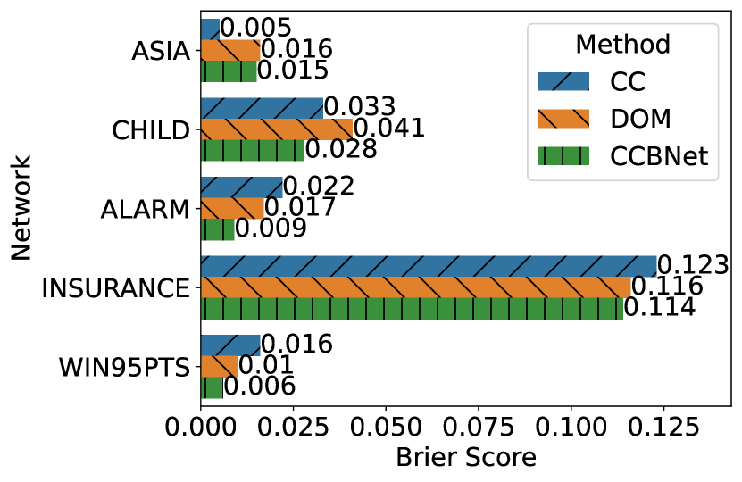
((a)) Brier scores relative to original network, related splits

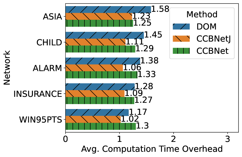
((b)) Average computation time overhead relative to original network, related splits

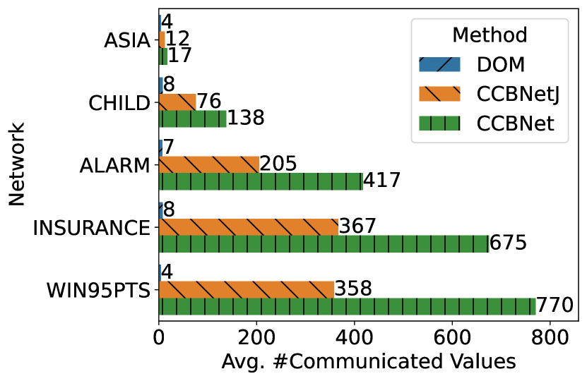
((c)) Average #communicated values rounded to nearest integer, related splits

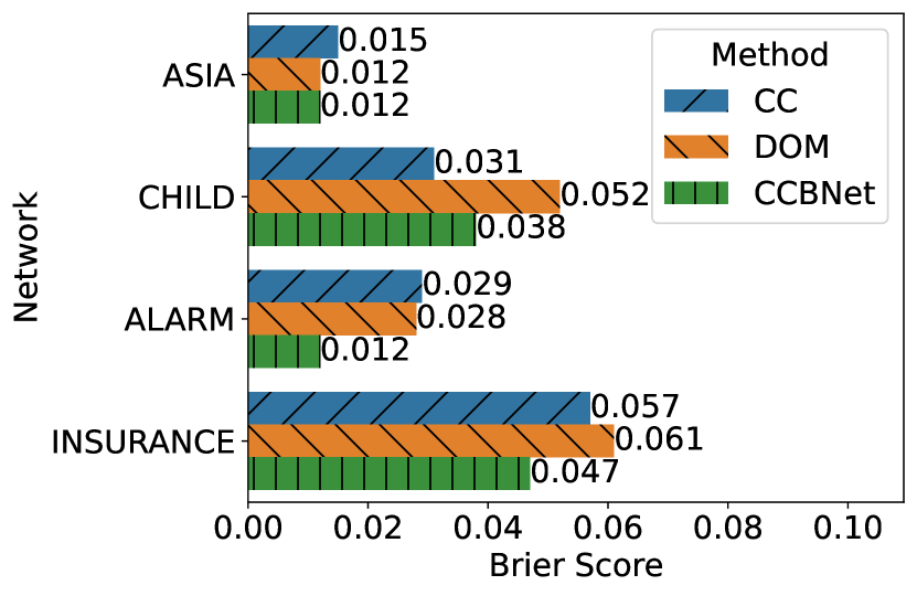
((d)) Brier scores relative to original network, random splits

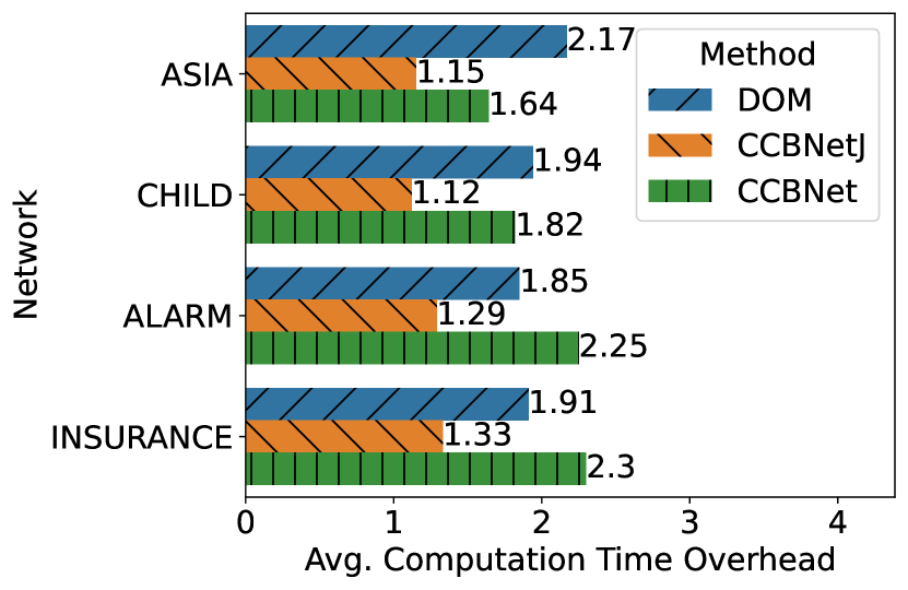
((e)) Average computation time overhead relative to original network, random splits

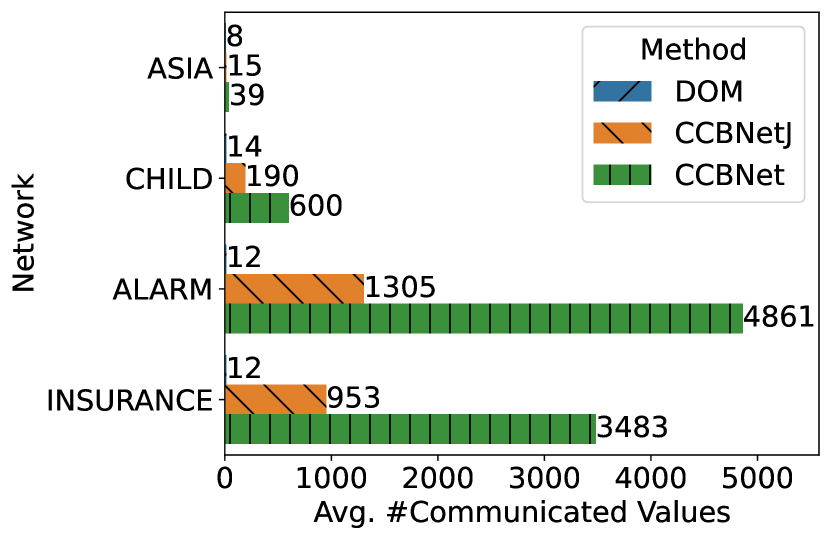
((f)) Average #communicated values rounded to nearest integer, random splits

Figure 3: Results for 4 parties, 30% of vars in >1 party (lower is better for all)

4.1 Setup

Our experiments evaluate average predictive performance, computation overhead, and communication cost of inference in single-machine simulations. We measure prediction quality via the Brier Score ($=\frac{1}{N}\sum^{N}_{t=1}\sum^{R}_{i=1}(f_{ti}-o_{ti})^{2}$ where $N$ is the number of queries, $R$ is the number of target variables state combinations, while $f$ and $o$ are predicted and reference probabilities). We report the total processing time ratio between examined methods and the ground truth network for computation overhead. For communication we consider the count of factor values exchanged per query. We do not evaluate CABN time or communication as we expect it to be amortizable.

We test on public networks (Table 1), consider two variable splitting methods, and multiple overlap variable ratios. Related splits assign to parties variables connected in the ground truth network. Random splits ensure parties have equal variable counts and share the same overlaps. Test sets contain 2000 queries, each with one random overlap variable as the target and 60% of the others fixed as evidence. Related splits attempt to simulate a realistic deployment in which the experts within clients have an incomplete but close-to-the-ground truth view of the interactions between their modeled variables (which also differ in number). Random splits aim for a worst-case scenario where the variables within clients (of roughly equal number) are not subgraphs of the complete network, generally giving more densely connected local networks and overlaps, as a worst-case scenario.

4.2 Baselines

As the closest prior work is strictly centralized, our baselines are:

Centralized Combination (CC) iteratively combines parties by the method of [12] and treats the network as an MRF if cycles form.

Centralized Union (CU), the approach confidentially mimicked by CCBNet, is structurally based on the union of [11], combines parameters via geometric mean, and also applies the MRF principle.

Decentralized Output Mean (DOM) is a naïve approach that takes the geometric mean for each target variable’s state probabilities over independently operating contained parties. It trades modeling long-range effects for confidentiality.

CCBNetJ is a degenerate CCBNet variant that stores the fully combined central CPDs for overlaps in one of the concerned parties, trading some safety for faster inference.

4.3 CCBNet Performance Overview

Here, we summarize the Brier score, computation time, and communication overhead of CCBNet under two splitting methods, different overlapping ratios (10%, 30%, and 50%), and the party number (2, 4, and 8). Due to the space limitations, we present the full results in the appendix and highlight in Figure 3 the performance trend via the representative case of four parties with a 30% overlap ratio.

Predictive Performance. Regardless of split type, CCBNet predictions often outperform or match the classic CC and always beat the naïve DOM. Figure 3(a) gives results for related splits, CCBNet only scores worse than CC on the smallest network (0.015 versus 0.005) and gains a significant advantage over the larger ones (0.022 versus 0.009, 0.123 versus 0.114, and 0.006 versus 0.016). CCBNet has an advantage over DOM in all scenarios. Examining the random splits in Figure 3(d), CCBNet still outscores CC in all but one of the smaller networks (0.031 vs 0.038) and maintains its lead over DOM in all but the smallest network, where the two tie. Since CCBNet yields the same predictive ability as its centralized counterpart CU, the differentiating points with CC are the structure combination policy and parameter combination operator. Over both splits, the pairing of the union selection and geometric mean aggregation in CCBNet fares better in most cases than the nondeterministic selection and superposition aggregation of CC, apart from some instances within small networks. Finally, complete test results confirm the expectation that adding more parties tends to decrease performance while increasing overlaps has the opposite effect.

Computation Overhead. Regarding computation cost relative to centralized inference on the original network, average slowdowns are 1.63x for DOM, 1.15x for CCBNetJ, and 1.6x for CCBNet. Communication latency is unaccounted for as it can vary greatly based on the deployment. Still, we overestimate wall time by summing computation time across parties, as much processing would happen concurrently in reality. In the related splits from Figure 3(b), across the board, CCBNetJ is the fastest, but others follow closely. CCBNet is the second best in all except the largest networks, where it fares worse than DOM (1.17x vs 1.3x slower). The networks also examined for random splits in Figure 3(e) show a similar trend, with somewhat higher general overhead, especially for CCBNet. Thus, as expected, CCBNetJ is faster than CCBNet, but both perform reasonably in most scenarios, even if the latter suffers more than the former as overlaps increase in complexity. The DOM implementation does seem to have a higher base overhead, but the gap to the other algorithms is often relatively contained. Further, complete results certify that adding parties improves speed while increasing overlaps decreases it. Regarding absolute total computation time, queries take the longest on the largest related splits dataset, with DOM averaging 2.9 ms/query, CCBNetJ 2.5 ms, and CCBNet 3.2 ms.

Communication Cost. Regarding the number of communicated CPD values per query, DOM averages merely 9, while CCBNetJ and CCBNet need orders of magnitude more at 387 and 1222, respectively. Since the number of communicated values depends on which party initiates a query, the reported figures include communication internal to the initiator to eliminate variability, tending to overestimate reality. The number of messages to complete a query is the same for all methods. Furthermore, the raw data transmitted in bytes remain in the low megabyte range for hundreds of thousands of values before compression. Figure 3(c) shows the mentioned discrepancy over related splits for all but the smallest network, in which the three methods are comparable. DOM merges complete party outputs and cannot propagate evidence between parties. Thus, it does not increase communication with the number of overlaps, and parties that do not contain any target variables send empty replies. The situation for random splits, illustrated in Figure 3(f), is very similar, although the disadvantage of CCBNet over CCBNetJ widens considerably. As for adding parties and increasing overlaps, the complete appendix results attest that both increase communication for all methods.

4.4 Party Weighting

#Parties		2				4
Vars in >1 Party		10%		30%		10%		30%
Method		UW	W	UW	W	UW	W	UW	W
Network	ASIA	0.028	0.018	0.029	0.009	0.036	0.020	0.031	0.011
	CHILD	0.067	0.067	0.088	0.047	0.084	0.067	0.097	0.048
	ALARM	0.063	0.058	0.061	0.050	0.103	0.092	0.061	0.057
	INSURANCE	0.079	0.104	0.051	0.051	0.112	0.088	0.135	0.098

Table 2: Unweighted (UW) & Weighted (W) Brier scores for CCBNet relative to original network - random splits, imbalanced learning data (lower is better)

Table 2 shows the weighted version of the proposed method having better predictive performance than the unweighted one in almost all scenarios with random splits. In weighting tests, we reduce the overall amount of data used for learning local BNs to ensure more variance and alternatingly assign parties a smaller or larger fraction of training data. Over the one scenario where the unweighted version performs better (0.079 versus 0.104), parties with lower data get overly punished for its perceived imprecision. Since each CPD has a single weight, all parents of a node within the party are still treated uniformly according to that value, even if there is a mismatch between the weight and the actual quality of the estimates. Similarly, if a party with lower overall confidence is the only one to model a highly-influential parent, its importance is slightly misrepresented in the final result. Nevertheless, although the strength of the effect has a considerably high variance, weighting has a clear positive overall impact in tested scenarios.

4.5 Large Networks & Many Parties

Networks/	Brier Score			Avg Comp Time Overhead			Avg #Comm Values
Parties	CC	DOM	CCBNet	DOM	CCBNetJ	CCBNet	DOM	CCBNetJ	CCBNet
ANDES/16	0.040	0.039	0.035	0.58	0.62	0.68	4	317	445
PIGS/32	0.103	0.092	0.076	0.39	0.51	1.34	7	4202	37838
LINK/64	0.144	0.125	0.126	0.25	0.35	0.39	6	2402	4549
MUNIN2/128	0.016	0.015	0.015	0.20	0.41	0.67	11	88581	242788

Table 3: Metrics for large networks & many parties - related splits, 10% of vars in >1 party (lower is better for all)

Lastly, in Table 3, our tests for challenging use cases with large networks (223-1003 features), many parties (16-28), and related variable splits, but lower overlaps reconfirm prediction/communication trends, yet computation improves over original networks. As previously, in larger networks, CCBNet’s predictions outperform CC, and communication size increases with parties and network size, averaging 71k values/request. Computation overhead is always <1 (i.e., a speedup) by 21% on average, as the hardness of inference makes approximating a big network by splitting it into chunks faster, even before considering parallel party solving.

5 Attacks on CCBNet

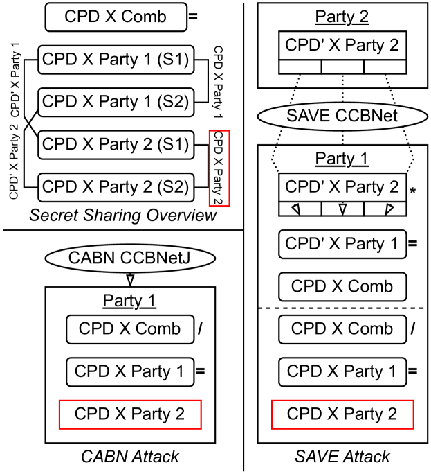
Figure 4: Visualization of showcased CABN & SAVE attacks

To recap, a classic combination of related BNs, which encode confidential information into a single global model, has a very high risk of leaking information to all parties with direct access to it. As exemplified in the middle pane of Figure 1, even at a purely structural level, the centralized combination can contain much, if not all, of the local party information. Furthermore, at a parameter level, probability functions for any non-overlap nodes remain unmodified. Since BNs are human-readable, inspection can compromise sensitive information even before any inference.

We briefly review two attacks to reconstruct CPDs during CABN and SAVE, respectively, along with their implications in CCBNet and CCBNetJ. The attacks do not bypass the obfuscation of unowned variable names and states but still expose potentially sensitive information via the recovered probability values. We successfully execute them, as visualized in Figure 4, on a corner case of two-party ASIA and CHILD network instances.

CABN Attack. The first attack allows a party to reconstruct a peer’s CPD for an overlap variable without inference, assuming no other parties are involved in the overlap, the attacker holds the combined CPD, and the protocol is CCBNetJ. The attacker starts by running CABN until it computes the combined CPD. Then, it removes its contribution from the geometric product that yielded the CPD, marginalizes any parents that should not be present in the victim’s version, and normalizes to get the final result. With any secure computation scheme, if one of two input parties knows the output and the reversible operations applied, it can find the other input. For overlaps with three or more parties, the attacker can only reconstruct an aggregation of the other involved CPDs. Even when the attack is possible, name obfuscation still hides the real-world meaning of the variables previously unknown to the attacker. Should any party outside the overlap exist, in the assumed no collusion setting, having it compute and store the combined CPD instead gives a minimum-change fix. CCBNet is not vulnerable, as it does not join shares before applying inference operations.

SAVE Attack. The second attack allows a party to reconstruct a peer’s CPD for an overlap variable via inference, still assuming that the overlap contains no other parties but also applies to CCBNet. The attacker, who can be either of the two parties in the overlap, begins by querying for the overlap variable as the only target, specifying a state for each of its parents in the evidence. With all parents fixed, no other variables in the victim’s network can affect the transmitted result. Thus, the attacker receives one row from the victim’s share of the combined target CPD. Consequently, the attacker repeats the procedure for all other combinations of parent states, building up the victim’s complete CPD share. It then takes the product of its share, and the one recovered from the other party to obtain the full combined CPD. Finally, like in the previous attack, it removes the contribution of its initial CPD (not the secret share) from the combination, marginalizes any parents not in the victim, and normalizes to find the result. Also similar to the previous attack, obfuscation limits the damage that can be done, while with the involvement of more than two parties, the attacker is able to compromise their shares, but not the contribution of each, before sharing the secrets. Thus, secret sharing avoids the attack for overlaps with three or more parties. As the attack requires a series of specific queries, redundant in most real applications, a simple defense has parties set a limit on the number of requests serviced that target a node with all parents in the evidence.

6 Discussion

Framework Flexibility. As outlined through the rest of the work, the framework naturally supports more variations than the presented CCBNet and CCBNetJ, allowing for a choice between increased confidentiality measures or other performance criteria. One choice entails replacing the HE with an SSS in CABN to swap computation by communication. Another is disallowing specific two-party overlap queries to avoid compromising network parameters. Of course, picking CCBNetJ for its speed or, conversely, CCBNet for its safety is perhaps the clearest such example.

For all variants above, changing SAVE line 4 to VarElim(Q, {}, auxFacts, True) so that inner variable elimination calls return the product of leftover factors instead of their set further increases security safeguards at the cost of overhead. Since the factors do not share variables, their product creates a comparatively much larger output to transmit. Nevertheless, it also makes it harder for the receiver to gain insight into the sender’s independent variables.

Framework Applicability. Although our motivating use case comes from semiconductor manufacturing, we devise CCBNet to be as generally applicable as possible, even outside other manufacturing industries. Hence, we also base our evaluation on public data sets. Future improvements to further aid such goals could be confidentially harnessing available observed data samples within parties when updating overlap variable representation, or allowing additional types of workloads on the representation (e.g., approximate inference).

7 Conclusion

We propose CCBNet to address the issue of collaborative analysis for BNs in confidential (manufacturing) settings. The framework allows distributed analysis spanning involved models without revealing their contents. It has no model compatibility restrictions and allows unequally weighting parties. We extensively evaluate the method and a lower-overhead but less robust variant, CCBNetJ, against non-confidential central approaches and a naïve, distributed, confidential formulation. Results show CCBNet outperforming/matching the naïve/centralized approaches while maintaining reasonable computation time that decreases to 23% of centralized formulations in large networks with many parties but produces much larger messages than minimum-interaction distributed alternatives, averaging 71k communicated values/request. Altogether, CCBNet offers centralized-like predictive performance in a distributed setting and ensures a base for protecting parties’ private information.

Appendix A Experiment Method & Results Details

#Parties		2									4						8
Vars in >1 Party		10%			30%			50%			10%			50%			10%			30%			50%
Method		CC	DOM	CCBNet	CC	DOM	CCBNet	CC	DOM	CCBNet	CC	DOM	CCBNet	CC	DOM	CCBNet	CC	DOM	CCBNet	CC	DOM	CCBNet	CC	DOM	CCBNet
Network	ASIA	0.011	0.022	0.006	0.011	0.022	0.006	0	0.015	0.001	0.005	0.016	0.015	0.013	0.021	0.017	0.076	0.076	0.076	0.076	0.076	0.076	0.055	0.054	0.054
	CHILD	0.002	0.034	0.002	0.001	0.02	0.001	0.001	0.02	0.001	0.08	0.106	0.08	0.012	0.033	0.011	0.165	0.173	0.164	0.071	0.09	0.072	0.044	0.046	0.023
	ALARM	0.001	0.016	0.005	0.001	0.016	0.005	0.001	0.016	0.005	0.027	0.047	0.029	0.02	0.012	0.011	0.04	0.074	0.038	0.029	0.041	0.026	0.039	0.022	0.017
	INSURANCE	0.007	0.022	0.009	0.015	0.017	0.011	0.013	0.01	0.008	0.111	0.117	0.108	0.086	0.037	0.032	0.154	0.166	0.153	0.189	0.135	0.131	0.091	0.085	0.077
	WIN95PTS	0.015	0.007	0.001	0.01	0.007	0.005	0.01	0.007	0.005	0.019	0.011	0.005	0.01	0.007	0.004	0.026	0.016	0.011	0.038	0.016	0.011	0.016	0.013	0.006

Table 4: Brier score relative to original Network - related splits (lower is better)

#Parties		2									4						8
Vars in >1 Party		10%			30%			50%			10%			50%			10%			30%			50%
Method		DOM	CCBNetJ	CCBNet	DOM	CCBNetJ	CCBNet	DOM	CCBNetJ	CCBNet	DOM	CCBNetJ	CCBNet	DOM	CCBNetJ	CCBNet	DOM	CCBNetJ	CCBNet	DOM	CCBNetJ	CCBNet	DOM	CCBNetJ	CCBNet
Network	ASIA	1.29	0.93	1.07	1.53	1.11	1.26	1.61	1.1	1.31	1.74	1.11	1.27	1.85	1.12	1.42	1.56	1.04	1.18	1.72	1.15	1.29	2.01	1.17	1.46
	CHILD	1.16	1.01	1.07	1.39	1.02	1.19	1.4	1.03	1.2	1.2	1.0	1.11	1.72	1.15	1.54	1.26	1.01	1.07	1.5	1.03	1.25	2.06	1.13	1.81
	ALARM	1.12	0.98	1.08	1.13	0.99	1.08	1.16	0.98	1.05	1.11	0.99	1.07	1.44	1.1	1.44	1.12	0.98	1.06	1.36	1.13	1.34	1.79	1.24	1.89
	INSURANCE	1.18	0.99	1.09	1.36	1.07	1.31	1.56	1.11	1.49	1.18	1.06	1.19	1.66	1.2	1.65	1.2	1.02	1.17	1.34	1.05	1.31	1.8	1.13	1.73
	WIN95PTS	1.03	0.92	1.01	1.13	0.96	1.11	1.13	0.97	1.13	0.93	0.89	0.97	1.28	1.09	1.49	0.89	0.85	0.91	1.18	1.04	1.37	1.45	1.08	1.73

Table 5: Average computation time overhead relative to original network - related splits (lower is better)

#Parties		2									4						8
Vars in >1 Party		10%			30%			50%			10%			50%			10%			30%			50%
Method		DOM	CCBNetJ	CCBNet	DOM	CCBNetJ	CCBNet	DOM	CCBNetJ	CCBNet	DOM	CCBNetJ	CCBNet	DOM	CCBNetJ	CCBNet	DOM	CCBNetJ	CCBNet	DOM	CCBNetJ	CCBNet	DOM	CCBNetJ	CCBNet
Network	ASIA	4	16	22	4	16	22	4	16	24	4	12	17	4	14	23	4	11	15	4	11	15	4	12	20
	CHILD	10	64	80	7	72	109	7	72	109	10	47	63	9	120	269	10	43	59	8	60	95	10	189	604
	ALARM	5	65	93	5	65	93	5	65	93	6	100	146	7	484	1038	6	136	205	6	227	437	8	768	2070
	INSURANCE	8	117	173	7	254	417	7	359	633	9	432	807	8	482	979	9	274	509	8	279	526	9	361	786
	WIN95PTS	4	175	262	4	274	440	4	274	440	4	139	200	4	459	1000	4	115	158	5	344	1029	5	456	1588

Table 6: Average #communicated values rounded to nearest integer - related splits (lower is better)

Metric		Brier Score									Average Computation Time Overhead									Average #Communicated Values
#Parties		2						4			2						4			2						4
Vars in >1 Party		10%			30%			10%			10%			30%			10%			10%			30%			10%
Method		CC	DOM	CCBNet	CC	DOM	CCBNet	CC	DOM	CCBNet	DOM	CCBNetJ	CCBNet	DOM	CCBNetJ	CCBNet	DOM	CCBNetJ	CCBNet	DOM	CCBNetJ	CCBNet	DOM	CCBNetJ	CCBNet	DOM	CCBNetJ	CCBNet
Network	ASIA	0.021	0.012	0.012	0.011	0.006	0.006	0.029	0.023	0.023	1.18	0.92	1.0	1.49	1.08	1.24	1.73	1.19	1.47	4	11	15	4	11	16	8	16	38
	CHILD	0.031	0.021	0.023	0.027	0.02	0.018	0.029	0.047	0.031	1.23	1.06	1.13	1.36	1.08	1.33	1.37	1.07	1.34	6	97	146	7	153	254	12	80	202
	ALARM	0.009	0.013	0.011	0.006	0.008	0.005	0.025	0.043	0.022	1.13	0.98	1.06	1.31	1.07	1.29	1.27	1.15	1.69	5	189	304	6	423	691	11	714	2599
	INSURANCE	0.05	0.031	0.028	0.039	0.025	0.024	0.072	0.068	0.052	1.15	1.04	1.18	1.33	1.14	1.4	1.33	1.21	1.79	6	195	315	6	336	561	12	686	2464

Table 7: Results for random splits (lower is better for all)

Input: bnDAG, nrSplits, nrOverlaps, randGen
Output: Splits

1:  dfsTree $\leftarrow$ DFSTree(bnDAG)

2:  splits $\leftarrow$ GreedyModularityComms(DFSTree, nrSplits)[7]

3:  shuffledEdges $\leftarrow$ randGen.shuffle(bnDAG.edges)

4:  initNodeSplit $\leftarrow$ {}

5:  for splitNr $\leftarrow$ 1 $\dots$ nrSplits do

6:     for node $\leftarrow$ splits[nrSplit] do

7:        initNodeSplit[node] $\leftarrow$ splitNr

8:  ovNodes $\leftarrow$ { }

9:  connSplits $\leftarrow$ { }

10:  extraEdges $\leftarrow$ [ ]

11:  for nodeO, nodeI $\leftarrow$ shuffledEdges do

12:     if $|$ovNodes$|$ $\geq$ nrOverlaps then

13:        break

14:     es $\leftarrow$ {initNodeSplit[nodeO], initNodeSplit[nodeI]}

15:     if $|$es$|$ == 1 then

16:        continue

17:     if $|$connSplits$|$ < nrSplits AND es $\subseteq$ connSplits then

18:        extraEdges += (nodeO, nodeI)

19:     else

20:        ovNodes $\cup$= {nodeO, nodeI}

21:        connSplits $\cup$= es

22:        splits[initNodeSplit[nodeO]] $\cup$= {nodeO}

23:        splits[initNodeSplit[nodeI]] $\cup$= {nodeI}

24:  for nodeO, nodeI $\leftarrow$ extraEdges do

25:     if $|$ovNodes$|$ $\geq$ nrOverlaps then

26:        break

27:     ovNodes $\cup$= {nodeO, nodeI}

28:     splits[initNodeSplit[nodeO]] $\cup$= {nodeO}

29:     splits[initNodeSplit[nodeI]] $\cup$= {nodeI}

30:  return  splits

Algorithm 3 Related Split

Input: bnDAG, nrSplits, nrOverlaps, randGen
Output: Communities

1:  shuffledNodes $\leftarrow$ randGen.shuffle(bnDAG.nodes)

2:  ovs $\leftarrow$ randGen.sample(shuffledNodes, nrOverlaps)

3:  splits $\leftarrow$ SplitEqualParts(shuffledNodes, nrSplits)

4:  for split $\leftarrow$ splits do

5:     split $\cup$= ovs

6:  return  splits

Algorithm 4 Random Split

We detail the procedures used for related and random splits of ground truth variables amongst parties, used throughout all experiments, in Algorithm 3 and Algorithm 4, respectively. Table 4, Table 5, and Table 6. Regarding additional experiment results with related splits, Table 4 covers predictive performance, Table 5 covers computation overhead, and Table 6 covers communication cost. In a few networks under related splits, adjacent overlap figures (e.g., 30% and 50%) have the same splits and inherently score, either because of the small number of nodes (ASIA) or because all possible overlaps for the given topology are formed (CHILD, ALARM). Table 7 shows extra results for all three metrics under random splits. For choosing the order of variable elimination during inference, we use a min weight heuristic, which greedily chooses a variable such that the product of factors containing it has the smallest size.

We run each experiment once, with a fixed seed determining the randomness for sampling data instances from the reference network and splitting it into overlapping variables sets of parties. We utilize an Intel(R) Core(TM) i9-12900KF CPU @ 3.20GHz (note that inference in the single-machine simulation is single-threaded), with 120 GB of RAM, and Ubuntu 20.04.6 LTS as the OS. We implement the codebase in Python 3.10, using pgmpy 0.1.24 as the backbone for BNs in our framework, tenseal 0.3.14 for homomorphic encryption, and openmined.psi 2.0.2 for private set intersection. We provide the code as supplementary material.

Appendix B Multiplication-based Secret Sharing

Definition 1 (Group).

A group [17] is a set $G(\neq\emptyset)$ and operation $\bullet:G\times G\longrightarrow G$ such that:

1. Asociativity: $a\bullet(b\bullet c)=(a\bullet b)\bullet c,\forall a,b,c\in G$

2. Neutral element: $\exists!e\in G$ such that $e\bullet a=a\bullet e=a,\forall a\in G$

3. Inverse element:$a\bullet a^{\prime}=a^{\prime}\bullet a=e,\forall a\in G,\exists!a^{\prime}$, where $e$ is the neutral element

Definition 2 ($\mathbb{Z}_{n}$).

$\mathbb{Z}_{n}$ is a group under $\{0,1,\dots,n-1\}$ and addition modulo (%) $n$.

Definition 3 ($\mathbb{Z}_{p}^{*}$).

$\mathbb{Z}_{p}^{*}$, for $p$ prime, is a group under $\{1,2,\dots,p-1\}$ and multiplication modulo (%) $p$.

Proposition 1.

The inverse $x^{\prime}$ of $x\in\mathbb{Z}_{p}^{*}$ is $x^{p-2}\%p$.

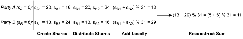
Figure 5: Example of computing the sum of two parties’ additively secret shared variables in $\mathbb{Z}_{31}$

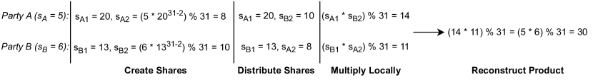
Figure 6: Example of computing the product of two parties’ multiplication-based secret shared variables in $\mathbb{Z}_{31}^{*}$

Secret sharing schemes are a family of methods that allow the distribution of a secret value among a group of parties by assigning each a share that does not yield any information about the secret but can, when pooled with enough others, reveal it [8]. The following details the classic additive scheme and the multiplication-based version used for CCBNet, relating them to each other.

Not leaking any information about a secret with theoretical guarantees for an adversary of unbounded computation requires sampling it from a uniform distribution, which is impossible for any infinite set, like $\mathbb{Z}$ or any subset of $\mathbb{R}$. Thus, most schemes perform their computation within (derivatives of) finite integer groups (Definition 1) large enough to contain all possibly required values for computations on the secrets. The previously mentioned fixed-precision encoding is an usual method for incorporating floating-point values. Multiplication in linear schemes requires additional interaction between the parties. Usually, it involves the help of a secretly sharing an additional set of values $a,b,c$, called Beaver triples [3], obeying $a*b=c$, with $a$ and $b$ chosen arbitrarily. Protocols exist for parties to generate triples amongst themselves securely, but a trusted third party can simplify the procedure.

Additive [17] secret sharing is a popular scheme in literature, which is defined on $\mathbb{Z}_{n}$ (Definition 2), with information-theoretic security for up to $n-1$ passively corrupt parties. Figure 5 exemplifies adding two parties’ secret values. Shamir’s secret sharing has a configurable $(t,n)$ threshold scheme, which produces secret shares based on a polynomial whose constant coefficient is the secret, and all others are random. It has information-theoretic security for up to $\lfloor n/2\rfloor$ passive corrupt parties and $\lfloor n/3\rfloor$ active ones. It uses Beaver triples to allow multiplication.

The multiplication-based scheme utilized in CCBNet is similar to the additive one but becomes non-linear by swapping efficient share addition for multiplication. As it works under $\mathbb{Z}_{p}^{*}$ (Definition 3), not $\mathbb{Z}_{n}$, instead of agreeing on a large enough $n$, parties agree on a large enough prime $p$ to instantiate the group. As in the additive case, to split a secret $s$ into $k$ shares, parties get shares $s_{1}$ through $s_{k-1}$ by uniformly sampling the group’s set of values and fix $s_{k}=s\bullet(s_{1}\bullet...\bullet s_{k-1})^{\prime}$. From Proposition 1, it follows that $s_{k}=s*(s_{1}*...*s_{k-1})^{p-2}$, where all multiplications are modulo $p$. Modular exponentiation can be efficiently computed even for large exponents. Reconstruction still happens by applying the group operator to all shares. Note that, although $0\notin\mathbb{Z}_{p}^{*}$, assuming that the party holding the secret keeps one of the shares, it can set its share to $0$, and sample $\mathbb{Z}_{p}^{*}$ for the remaining ones. Figure 6 gives a small example of multiplying two parties’ secret values.

References

- Abyaneh et al. [2022] A. Abyaneh, N. Scherrer, P. Schwab, S. Bauer, B. Schölkopf, and A. Mehrjou. Fed-cd: Federated causal discovery from interventional and observational data, 2022. URL https://arxiv.org/abs/2211.03846.
- Alrajeh et al. [2020] D. Alrajeh, H. Chockler, and J. Y. Halpern. Combining experts’ causal judgments. Artificial Intelligence, 288:103355, 2020. ISSN 0004-3702. https://doi.org/10.1016/j.artint.2020.103355. URL https://www.sciencedirect.com/science/article/pii/S0004370220301065.
- Beaver [1992] D. Beaver. Efficient multiparty protocols using circuit randomization. In J. Feigenbaum, editor, Advances in Cryptology — CRYPTO ’91, pages 420–432, Berlin, Heidelberg, 1992. Springer Berlin Heidelberg. ISBN 978-3-540-46766-3.
- Boneh et al. [2011] D. Boneh, A. Sahai, and B. Waters. Functional encryption: Definitions and challenges. In Y. Ishai, editor, Theory of Cryptography, pages 253–273, Berlin, Heidelberg, 2011. Springer Berlin Heidelberg. ISBN 978-3-642-19571-6.
- Campbell and How [2014] T. Campbell and J. P. How. Approximate decentralized bayesian inference, 2014.
- Cheon et al. [2017] J. H. Cheon, A. Kim, M. Kim, and Y. Song. Homomorphic encryption for arithmetic of approximate numbers. In T. Takagi and T. Peyrin, editors, Advances in Cryptology – ASIACRYPT 2017, pages 409–437, Cham, 2017. Springer International Publishing. ISBN 978-3-319-70694-8.
- Clauset et al. [2004] A. Clauset, M. E. J. Newman, and C. Moore. Finding community structure in very large networks. Physical Review E, 70(6), dec 2004. 10.1103/physreve.70.066111. URL https://doi.org/10.1103%2Fphysreve.70.066111.
- Cramer et al. [2015] R. Cramer, I. B. Damgård, and J. B. Nielsen. Secure Multiparty Computation and Secret Sharing. Cambridge University Press, 2015. 10.1017/CBO9781107337756.
- Daly et al. [2011] R. Daly, Q. Shen, and S. Aitken. Learning bayesian networks: approaches and issues. The knowledge engineering review, 26(2):99–157, 2011.
- De Cristofaro and Tsudik [2010] E. De Cristofaro and G. Tsudik. Practical private set intersection protocols with linear complexity. In R. Sion, editor, Financial Cryptography and Data Security, pages 143–159, Berlin, Heidelberg, 2010. Springer Berlin Heidelberg.
- Del Sagrado and Moral [2003] J. Del Sagrado and S. Moral. Qualitative combination of bayesian networks. International Journal of Intelligent Systems, 18(2):237–249, 2003. https://doi.org/10.1002/int.10086. URL https://onlinelibrary.wiley.com/doi/abs/10.1002/int.10086.
- Feng et al. [2014] G. Feng, J.-D. Zhang, and S. Shaoyi Liao. A novel method for combining bayesian networks, theoretical analysis, and its applications. Pattern Recognition, 47(5):2057–2069, 2014. ISSN 0031-3203. https://doi.org/10.1016/j.patcog.2013.12.005. URL https://www.sciencedirect.com/science/article/pii/S0031320313005232.
- Gao et al. [2021] E. Gao, J. Chen, L. Shen, T. Liu, M. Gong, and H. Bondell. Feddag: Federated dag structure learning, 2021. URL https://arxiv.org/abs/2112.03555.
- Gholami et al. [2016] B. Gholami, S. Yoon, and V. Pavlovic. Decentralized approximate bayesian inference for distributed sensor network. Proceedings of the AAAI Conference on Artificial Intelligence, 30(1), Feb. 2016. 10.1609/aaai.v30i1.10201. URL https://ojs.aaai.org/index.php/AAAI/article/view/10201.
- Goldreich [2005] O. Goldreich. Foundations of cryptography – a primer. Foundations and Trends® in Theoretical Computer Science, 1(1):1–116, 2005. ISSN 1551-305X. 10.1561/0400000001. URL http://dx.doi.org/10.1561/0400000001.
- Huang et al. [2022] J. Huang, K. Yu, X. Guo, F. Cao, and J. Liang. Towards privacy-aware causal structure learning in federated setting, 2022. URL https://arxiv.org/abs/2211.06919.
- [17] D. Kales. Secret sharing. URL https://www.iaik.tugraz.at/wp-content/uploads/teaching/mfc/secret_sharing.pdf.
- Kilbertus et al. [2018] N. Kilbertus, A. Gascon, M. Kusner, M. Veale, K. Gummadi, and A. Weller. Blind justice: Fairness with encrypted sensitive attributes. In J. Dy and A. Krause, editors, Proceedings of the 35th International Conference on Machine Learning, volume 80 of Proceedings of Machine Learning Research, pages 2630–2639. PMLR, 10–15 Jul 2018. URL https://proceedings.mlr.press/v80/kilbertus18a.html.
- Kim and Ghahramani [2012] H.-C. Kim and Z. Ghahramani. Bayesian classifier combination. In N. D. Lawrence and M. Girolami, editors, Proceedings of the Fifteenth International Conference on Artificial Intelligence and Statistics, volume 22 of Proceedings of Machine Learning Research, pages 619–627, La Palma, Canary Islands, 2012. PMLR. URL https://proceedings.mlr.press/v22/kim12.html.
- Koller and Friedman [2009] D. Koller and N. Friedman. Probabilistic graphical models: principles and techniques. MIT press, 2009.
- Li [2009] S. Z. Li. Markov random field modeling in image analysis. Springer Science & Business Media, 2009.
- Nannapaneni et al. [2016] S. Nannapaneni, S. Mahadevan, and S. Rachuri. Performance evaluation of a manufacturing process under uncertainty using bayesian networks. Journal of Cleaner Production, 113:947–959, 2016. ISSN 0959-6526. https://doi.org/10.1016/j.jclepro.2015.12.003. URL https://www.sciencedirect.com/science/article/pii/S0959652615018144.
- Ng and Zhang [2021] I. Ng and K. Zhang. Towards federated bayesian network structure learning with continuous optimization, 2021. URL https://arxiv.org/abs/2110.09356.
- Pavlin et al. [2010] G. Pavlin, P. de Oude, M. Maris, J. Nunnink, and T. Hood. A multi-agent systems approach to distributed bayesian information fusion. Information Fusion, 11(3):267–282, 2010. ISSN 1566-2535. https://doi.org/10.1016/j.inffus.2009.09.007. URL https://www.sciencedirect.com/science/article/pii/S1566253509000864. Agent-Based Information Fusion.
- Pearl [2009] J. Pearl. Causality. Cambridge University Press, 2 edition, 2009. 10.1017/CBO9780511803161.
- Russell [2010] S. J. Russell. Artificial intelligence a modern approach. Pearson Education, Inc., 2010.
- Scutari and Denis [2021] M. Scutari and J.-B. Denis. Bayesian networks: with examples in R. CRC press, 2021.
- Stephenson [2000] T. A. Stephenson. An introduction to bayesian network theory and usage. Technical report, Idiap, 2000.
- Tedesco et al. [2006] R. Tedesco, P. Dolog, W. Nejdl, and H. Allert. Distributed bayesian networks for user modeling. In T. Reeves and S. Yamashita, editors, Proceedings of E-Learn: World Conference on E-Learning in Corporate, Government, Healthcare, and Higher Education 2006, pages 292–299, Honolulu, Hawaii, USA, 10 2006. Association for the Advancement of Computing in Education (AACE). URL https://www.learntechlib.org/p/23699.
- van Daalen et al. [2022] F. van Daalen, L. Ippel, A. Dekker, and I. Bermejo. Vertibayes: Learning bayesian network parameters from vertically partitioned data with missing values, 2022. URL https://arxiv.org/abs/2210.17228.
- Yang [2020] W.-T. Yang. An Integrated Physics-Informed Process Control Framework and Its Applications to Semiconductor Manufacturing. Theses, Université de Lyon, Jan. 2020. URL https://theses.hal.science/tel-03461289.
- Ypma et al. [2018] A. Ypma, A. C. M. Koopman, and S. A. Middlebrooks. Methods & apparatus for obtaining diagnostic information, methods & apparatus for controlling an industrial process, Feb 2018.