Estimation and goodness-of-fit testing for positive random variables with explicit Laplace transform

Abstract

Many flexible families of positive random variables exhibit non-closed forms of the density and distribution functions and this feature is considered unappealing for modelling purposes. However, such families are often characterized by a simple expression of the corresponding Laplace transform. Relying on the Laplace transform, we propose to carry out parameter estimation and goodness-of-fit testing for a general class of non-standard laws. We suggest a novel data-driven inferential technique, providing parameter estimators and goodness-of-fit tests, whose large-sample properties are derived. The implementation of the method is specifically considered for the positive stable and Tweedie distributions. A Monte Carlo study shows good finite-sample performance of the proposed technique for such laws.

Keywords: Central Limit Theorem, consistent estimation, goodness-of-fit testing, Laplace transform, stable distribution, Tweedie distribution.

1 Introduction

Large classes of positive random variables display a simple closed form of the Laplace transform, even if their density functions can be solely given by means of special functions or series, which eventually require rather complex algorithms for their computation. Owing to this shortcoming, field scientists often discard the use of such random variables, although they are appropriate for modelling real data.

An archetype of such a class of laws is the positive stable distribution, which may be very suitable to model data with Paretian tails (see e.g. Nolan,, 2020). The density function of a positive stable random variable can be expressed by means of the Wright function (see e.g. Barabesi,, 2020), which unfortunately is awkward to compute (see the algorithms proposed by Luchko,, 2008). To this aim, Barabesi, (2020), Dunn and Smyth, (2005) and Dunn and Smyth, (2008) suggest some approximation methods based on ad-hoc Fourier or Laplace inversion techniques. However, these algorithms can be time-consuming and possibly inadequate for evaluating the maximum-likelihood estimates, especially when large dataset are at disposal. In this case, the maximum-likelihood method could be even prohibitive and alternative techniques are required.

Among these classes, the Tweedie distribution, owing to its flexibility, is useful for modelling data arising from a plethora of different frameworks (see e.g. Barabesi et al., 2016b, , Dunn and Smyth,, 2005, Tweedie et al.,, 1984). As a matter of fact, this family encompasses moderate heavy-tailed distributions, as well as light-tailed distributions and it also comprises the positive stable distribution as a special case (for more details, see the book of Nolan,, 2020). Actually, the Tweedie distribution is a tempered positive stable distribution. In addition, the Tweedie law may even model data with structural zeroes, since for some parameter ranges it is the mixture of the Dirac mass at zero and an absolutely-continuous positive distribution (see Aalen,, 1992). This feature is especially appealing when dealing with data arising from socio-economic or environmental phenomena (see Barabesi et al., 2016b, , Hasan and Dunn,, 2015), which indeed may produce structural zeroes. However, the distribution of a Tweedie random variable in turn involves the Wright function, giving rise to computational drawbacks.

In general, a large body of literature has been devoted to the tempering of heavy-tailed laws (see e.g. the monograph by Grabchak and Grabchak,, 2016). Indeed, even if heavy-tailed distributions are well-motivated models in a probabilistic setting, extremely fat tails may be unrealistic for many real applications. Such a drawback has led to the introduction of models which are morphologically similar to the original distributions, even if they display lighter tails. In this setting, large classes of tempered distributions may be formulated as scale mixtures of a Tweedie random variable with a mixturing positive random variable (see Barabesi et al., 2016a, , Torricelli et al.,, 2022). However, the corresponding density functions involve the generalized Mittag-Leffler function, which is even more challenging to compute that the Wright function (see Barabesi,, 2020 and references therein). In turn, the use of maximum-likelihood methods could be unfeasible for these models. Moreover, even least-square methods based on the theoretical and empirical Laplace or Fourier transforms could be inadequate, since they are likely to produce a criterion function which is not easily manageable, and possibly with multiple local minima. In addition, computational effort could be prohibitive for large datasets.

In this paper, we propose a suitable class of parameter estimators for positive random variables showing a simple Laplace transform. The proposed technique has connections with the procedures based on the probability generating function for integer-valued random variables by Di Noia et al., 2023a and Di Noia et al., 2023b . The consistency and the large-sample distribution of the suggested estimators are obtained, as well as estimators of their asymptotic variance, thus naturally allowing to introduce appropriate goodness-of-fit (GOF) test statistics. GOF tests are especially welcome for the considered class of models, as no such proposals are present in statistical literature.

The paper is organized as follows. In Section 2 some preliminaries and background remarks are given. In Section 3 the censoring strategy is described and the estimation procedure is introduced, as well as its asymptotic properties are derived. In Sections 4 and 5 the methodology is respectively adapted to the positive stable and Tweedie laws, and specific GOF tests are proposed. Section 6 is devoted to numerical experiments. Finally, conclusions are drawn in Section 7.

2 Preliminaries

Let us consider a positive random variable (r.v.) $X$ defined on the probability space $(\Omega,{\mathcal{A}},P)$ and let $L_{X}$ be the Laplace transform of $X$, i.e.

$$L_{X}(s)=E(e^{-sX})$$

for $s\geq 0$. Obviously, if $F$ is the cumulative distribution function of $X$, it holds $L_{X}(s)=\int_{0}^{1}F(-\log t/s)\,dt$ for $s>0$. Moreover, if $X$ is an absolutely-continuous random variable, we have $L_{X}(t)=\int_{0}^{\infty}e^{-sx}\,F^{\prime}(x)\,dx.$ A large distribution family has a Laplace transform of type

$$L_{X}(s)=g(s^{\gamma}),$$ (1)

where $\gamma$ is a parameter defined on a suitable subset of $\,]0,1]$, while $g$ is an appropriate function (see e.g. Barabesi,, 2020, Torricelli et al.,, 2022, and references therein). The family (1) includes some rather exotic distributions, such as the generalized Jacobi laws, which have Laplace transforms given by:

$$L_{X}(s)={{s^{\gamma}}\over{{\rm sinh}(s^{\gamma})}}$$

and

$$L_{X}(s)={{1}\over{{\rm cosh}(s^{\gamma})}},$$ (2)

where $\gamma\in\,]0,1/2]$ (see Biane et al.,, 2001 and Devroye,, 2009).

Example 1.

The family with Laplace transform given by (1) encompasses the positive stable distribution. Indeed, a positive stable r.v. has Laplace transform

$$L_{X}(s)=e^{-\lambda s^{\gamma}},$$ (3)

where $(\gamma,\lambda)\in\,]0,1]\,\times\,]0,\infty[$. For more details on the properties of this r.v. and its stochastic representations, see e.g. Devroye and James, (2014). The integer-valued counterpart of the positive stable distribution is considered in Barabesi and Pratelli, 2014b and Marcheselli et al., (2008). Parameter estimation for the positive stable distribution is discussed in depth in Section 4.

It should be remarked that $g$ could be in turn the Laplace transform of a further positive (not necessarily absolutely-continuous) r.v. $V$. More precisely, if

$$X=V^{1/\gamma}Z,$$

where $Z$ is a positive stable r.v. with parameters $(\gamma,1)$ independent of $V$ (i.e. $X$ is a scale mixture of positive stable distributions), we have

$$L_{X}(s)=E(e^{-sV^{1/\gamma}Z})=E(e^{-s^{\gamma}V})=L_{V}(s^{\gamma}).$$

Loosely speaking, in this setting the parameter $\lambda$ is assumed to be a positive r.v. with a suitable distribution. The resulting family encompasses many distributions as the positive Linnik distribution which is obtained when $V$ is distributed according to the Gamma distribution, see e.g. Barabesi et al., 2016a , Huillet, (2000) and Jose et al., (2010).

An even larger model family of distributions has a Laplace transform of type

$$L_{X}(s)=g((\theta+s)^{\gamma}-\theta^{\gamma}),$$ (4)

where $g$ is an appropriate function and $\theta\geq 0$. If $\theta>0$, the parameter $\gamma$ may also be defined on $\,]-\infty,1]$. Obviously, for $\theta=0$ the family given in (1) is obtained. In turn, the function $g$ in (4) could be a Laplace transform of a further positive r.v. $V$. These distribution classes of such a type are considered by Barabesi et al., 2016a , James, (2010) and Torricelli et al., (2022), among others.

Example 2.

The typical member of the family with Laplace transform given by (4) is the Tweedie distribution. Actually, a Tweedie r.v. has the Laplace transform

$$L_{X}(s)=e^{{\rm sgn}(\gamma)\lambda(\theta^{\gamma}-(\theta+s)^{\gamma})},$$ (5)

where $(\gamma,\lambda,\theta)\in\{[-\infty,0]\times\,]0,\infty[\times\,]0,\infty[\,\}\cup\{\,]0,1]\times\,]0,\infty[\times[0,\infty[\,\}$. The distribution has been popularized and analysed at length by Hougaard, (1986) and Jørgensen, (1987), following the seminal ideas described in Tweedie et al., (1984). The distribution is central in actuarial studies and ecology, among others (see e.g. Jørgensen,, 1987 and Kendall,, 2004). For its integer-valued counterpart, see Baccini et al., (2016) and Barabesi and Pratelli, 2014a . As to the random variate generation of a Tweedie r.v., see Barabesi and Pratelli, 2014b , Barabesi and Pratelli, (2015), and references therein. The family is very flexible and can be adopted as a model for datasets with complex and non-usual features, since it can simultaneously arrange fat tails and structural zeroes. The inferential issues for the Tweedie law will be discussed in details in Section 5.

Albeit the described families are very appealing from a probabilistic perspective, the drawback with their use consists in the complex structure of the corresponding density and distribution functions, despite the simple forms of their Laplace transform. Even if some approximations are available in order to compute maximum-likelihood estimates (as proposed by Barabesi,, 2020), their computation may be too time-consuming. Thus, alternative and simpler estimation methods may be welcome. These inferential methods should also produce GOF testing procedures which are particularly desirable, since no such proposals are present in literature.

3 Parameter estimation and GOF testing

Let the Laplace transform $L_{X}$ of the target random variable $X$ belong to the general class (4), specifically given by $L_{X}(s)=g\big{(}\lambda((\theta+s)^{\gamma}-\theta^{\gamma})\big{)},$ where $g$ is a suitable infinitely differentiable function on ${\mathbb{R}}\setminus\{0\}$, $\gamma\neq 0$ and $\lambda\kern-0.85358pt>\kern-0.85358pt0$. In particular, $E[X]$ is not finite for $\theta=0$, $\lambda>0$ and $\gamma\in\,]0,1[$. Our objective is to estimate parameters such as $\gamma$, $\lambda$, or $\gamma$, $\lambda$, $\theta$, and to obtain GOF test statistics by empirically estimating $L_{X}$ and its derivatives evaluated only at an ‘appropriate’ random point $A>0$.

Choosing a fixed deterministic point $a>0$ for calculating $L_{X}$ does not provide robust estimations of model parameters. This is because $L_{X}(a)$ could assume negligible values or values practically equal to one for many pairs of parameters $\lambda$ and $\gamma$, with $\theta=0$ or $\theta>0$, making any information on the parameters irrelevant. This drawback persists even when multiple values of $a$ are fixed deterministically and $L_{X}(a)$ or its standard empirical estimates are considered. To bypass this issue, in this section, we introduce a methodology that is broadly applicable to more general classes than (4), enabling robust and informative parameter estimations. In the following sections, we will illustrate these general results in detail for positive stable distributions and Tweedie distributions.

Let us start by noting that for any positive random variable $X$, the following relationship holds:

$$L_{X}^{(r)}(s)=(-1)^{r}E(X^{r}e^{-sX}),\qquad\forall s>0,\ \forall r\in\mathbb{N}.$$ (6)

In addition, let $T$ be a standard Exponential random variable, independent of $X$. By considering the further random variable $Y_{a}=X\mathbf{1}_{\{aX<T\}},$ where $a>0$ and $\mathbf{1}_{B}$ is the indicator function of the set $B$, it follows that

$$L_{Y_{a}}(s) =P(T\leq aX)+L_{X}(s+a)=1-L_{X}(a)+L_{X}(s+a).$$

The exponentially censored random variable $Y_{a}$ has a simple expression for its Laplace transform and moments. Even if $E(X)$ is not finite, for $a>0$ we have

$$E(Y^{r}_{a})=E(X^{r}e^{-aX})$$ (7)

thanks to (6). Thus, $Y_{a}$ may be more manageable than the original random variable $X$, as its moments are available. Equation (7) suggests considering $E(X^{r}e^{-aX})$ for a suitable $a$ when $L_{X}$ depends on some parameter to be estimated.

Remark 1.

If $L_{X}(s)=g\big{(}\lambda((\theta+s)^{\gamma}-\theta^{\gamma})\big{)}$, after some algebra, we also have

$$E(Y^{2}_{a})=E(Y_{a})^{2}{{g^{\prime\prime}((\theta+a)^{\gamma}-\theta^{\gamma})}\over{g^{\prime}((\theta+a)^{\gamma}-\theta^{\gamma})^{2}}}+E(Y_{a}){{1-\gamma}\over{\theta+a}},$$ (8)

and

$$\kern-7.68222ptE(Y^{3}_{a})\kern-1.70717pt=\kern-1.70717ptE(Y_{a})^{3}\,{{g^{\prime\prime\prime}((\theta\kern-1.13809pt+\kern-1.13809pta)^{\gamma}-\theta^{\gamma})}\over{g^{\prime}((\theta\kern-1.13809pt+\kern-1.13809pta)^{\gamma}-\theta^{\gamma})^{3}}}\kern-1.99168pt+\kern-1.99168pt{{1-\gamma}\over{\theta\kern-1.13809pt+\kern-1.13809pta}}\Big{(}3E(Y^{2}_{a})\kern-1.70717pt+\kern-1.70717ptE(Y_{a})\,{{2\gamma\kern-1.13809pt-\kern-1.13809pt1}\over{\theta+a}}\Big{)}.$$ (9)

To estimate the model parameters, a natural approach could rely on (6) by adopting the substitution principle based on the empirical counterpart of $E(X^{r}e^{-aX})$, where $r$ does not exceed the number of parameters. In practical applications, the number of parameters typically is $1$, $2$, or $3$, making this method feasible for implementation with real data.

However, the choice of $a$, denoted by $a_{*}$, is crucial for this purpose as discussed earlier in this section. The ‘optimal’ $a_{*}$ will depend on the model parameters, and we propose a data-driven method for obtaining a coherent estimator $A$ of $a_{*}$. To achieve this, first consider that $L_{X}([0,\infty[)=]p,1]$, where $p=P(X=0)$.

If $p=0$, to avoid $Y_{a_{*}}$ being too censored or scarcely censored and thus losing information on parameters, we could set $a_{*}=L_{X}^{-1}(c_{*})$ where $L^{-1}_{X}$ denotes the inverse function of $L_{X}$ and $c_{*}$ is an element of $[1/5,4/5]$. Moreover, in the setting of positive stable distribution, it is convenient to maximize $-c_{*}\log(c_{*})$ for estimating $\gamma$. Since $c_{*}=1/e$ is the maximum point, in the following, we will take

$$a_{*}=L_{X}^{-1}(1/e)$$

when $p=0$. Otherwise, $c_{*}$ will be chosen to be greater than $p$. Now, let $X_{1},\ldots,X_{n}$ be $n$ independent copies of the r.v. $X$ and let

$$L_{n}(s)={{1}\over{n}}\sum_{i=1}^{n}e^{-sX_{i}}$$

be the empirical counterpart of $L_{X}$. Denote $F_{n}$ as the empirical cumulative distribution function associated with $X_{1},\ldots,X_{n}$. It is worth noticing that for all $s>0$, it holds

$$|L_{X}(s)-L_{n}(s)|=\Big{|}\int_{0}^{1}\big{(}F(-\log t/s)-F_{n}(-\log t/s)\big{)}\,dt\Big{|}\leq||F-F_{n}||_{\infty}.$$

Moreover, let $A$ be a further positive random variable, which is a function of $X_{1},\ldots,X_{n}$ and is defined by the implicit equation

$$L_{n}(A)={{1}\over{n}}\sum_{i=1}^{n}e^{-AX_{i}}=e^{-1}.$$

when $p=0$. This implicit definition of $A$ ensures that $A$ is data-driven, making it adaptive to the sample data $X_{1},\ldots,X_{n}$. Since $\cap_{i=1}^{n}\{X_{i}>0\}$ is a negligible event when $p=0$, on the basis of the Glivenko-Cantelli Theorem, $A$ is well defined and converges almost surely to $a_{*}=L^{-1}_{X}(e^{-1})$ because

$$|L_{X}(A)-L_{X}(a_{*})|=|L_{X}(A)-1/e|=|L_{X}(A)-L_{n}(A)|\leq||F-F_{n}||_{\infty}.$$

If $p<1/e$, $A$ is well defined for large $n$ and the same asymptotic result holds true. Otherwise, if $p\geq 1/e$, we can consider $c_{*}=\frac{1+(e-1)p}{e}$ and define $A$ for large $n$ by the implicit equation

$$L_{n}(A)={{1}\over{n}}\sum_{i=1}^{n}e^{-AX_{i}}=\frac{1+(e-1)\widehat{p}_{n}}{e}$$

where $\widehat{p}_{n}={{1}\over{n}}\sum_{i=1}^{n}I_{\{X_{i}=0\}}$. For this choice of $c_{*}$ similar asymptotic results for $A$ are satisfied as when $c_{*}=1/e$. Additionally, we denote

$$m_{r,a_{*}}=E(Y_{a_{*}}^{r})=E(X^{r}e^{-a_{*}X})$$

with empirical counterpart

$$\widehat{m}_{r,A}={{1}\over{n}}\sum_{i=1}^{n}X_{i}^{r}e^{-AX_{i}}.$$

In the following Proposition we obtain the large-sample properties of the r.v.s $A$ and $\widehat{m}_{1,A},\ldots,\widehat{m}_{k,A}$, with $k\geq 1$, by means of a suitable use of the Delta Method.

Proposition 1.

If $p<1/e$ then the random vector $(\widehat{m}_{1,A},\ldots,\widehat{m}_{k,A},A)$ converges almost surely to the vector $(m_{1,a_{*}},\ldots,m_{k,a_{*}},a_{*})$, while the random vector

$$\sqrt{n}(\widehat{m}_{1,A}-m_{1,a_{*}},\ldots,\widehat{m}_{k,A}-m_{k,a_{*}},A-a_{*})$$

converges in distribution to the multivariate normal law $\mathrm{N}_{k+1}(0,\Sigma)$ as $n\to\infty$. Moreover, $\Sigma$ is the variance-covariance matrix of the random vector $(V_{1},\ldots,V_{k},W)$, with

$$V_{r}=e^{-a_{*}X}\Big{(}X^{r}-{{m_{r+1,a_{*}}}\over{m_{1,a_{*}}}}\Big{)},$$

for $r=1,\ldots,k$, and

$$W={{e^{-a_{*}X}}\over{m_{1,a_{*}}}}.$$

In particular, a consistent estimator of $\Sigma$ is given by the sample variance-covariance matrix of the random vectors $(\widehat{V}_{1,i},\ldots,\widehat{V}_{k,i},\widehat{W}_{i})$, $i=1,\ldots,n$, where

$$\widehat{V}_{r,i}=e^{-AX_{i}}\Big{(}X^{r}_{i}-{{\widehat{m}_{r+1,A}}\over{\widehat{m}_{1,A}}}\Big{)},\qquad\widehat{W}_{i}={{e^{-AX_{i}}}\over{\widehat{m}_{1,A}}}.$$

Proof.

For simplicity of notation, let us denote $a=a_{*}$. If $u=(u_{1},\ldots,u_{k})$ is an element of $\mathbb{R}^{k}$ and $t\in\mathbb{R}$, let us consider the r.v.

$$U_{n}=\sqrt{n}\Big{(}\sum_{r=1}^{k}u_{r}(\widehat{m}_{r,A}-m_{r,a})+t(A-a)\Big{)}.$$

On the basis of the Mean Value Theorem there exists a map $h$ defined on $]0,\infty[\,^{2}$ such that, for any $b,x>0$, it holds

$$e^{-bx}=e^{-ax}-xe^{-h(b,x)x}(b-a),$$

with $h(b,x)\in\,]\min(b,a),\max(b,a)[$. Thus, we have

$$U_{n}=\sqrt{n}\Big{(}\sum_{r=1}^{k}u_{r}(\widehat{m}_{r,a}-m_{r,a})+(A-a)(t-\sum_{r=1}^{k}{u_{r}\over n}\sum_{i=1}^{n}X_{i}^{r+1}e^{-h(A,X_{i})X_{i}})\Big{)}.$$

Since $A$ converges almost surely to $a$, the Law of Large Numbers and the Continuous Mapping Theorem imply that

$$\lim_{n}{1\over n}\sum_{i=1}^{n}X_{i}^{r+1}e^{-h(A,X_{i})X_{i}}=m_{r+1,a}$$

almost surely. Moreover, if $p=0$ there exists a negligible event $H$ such that $s\mapsto L_{n}(s)(\omega)$ is a decreasing function for any $\omega\in H^{c}$. These functions are invertible for any $\omega\in H^{c}$ and their inverse mappings are differentiable at $L_{n}(a)(\omega)$ with derivative $1/L^{\prime}_{n}(a)(\omega)$. Then $\sqrt{n}(A-a)$ coincides almost surely with

$$\sqrt{n}(L^{-1}_{n}(e^{-1})-L^{-1}_{n}(L_{n}(a)))\kern-1.70717pt=\kern-1.70717pt{{\sqrt{n}}\over{L^{\prime}_{n}(a)}}(e^{-1}-L_{n}(a))\kern-1.42262pt+\kern-1.42262pto_{P}(\sqrt{n}(e^{-1}-L_{n}(a)))$$

Since $L^{\prime}_{n}(a)$ converges almost surely to $-m_{1,a}$, and $o_{P}(\sqrt{n}(e^{-1}-L_{n}(a)))$ coincides with $o_{P}(\sqrt{n}(L_{X}(a)-L_{n}(a)))=\sqrt{n}(L_{X}(a)-L_{n}(a))o_{P}(1),$ from the convergence in distribution of $\sqrt{n}(L_{X}(a)-L_{n}(a))$ it follows that $U_{n}$ has the same large-sample behaviour of the r.v.

$$S_{n}=\sqrt{n}\Big{(}\sum_{r=1}^{k}u_{r}(\widehat{m}_{r,a}-m_{r,a})+{{1}\over{m_{1,a}}}(L_{n}(a)-e^{-1})(t-\sum_{r=1}^{k}u_{r}m_{r+1,a})\Big{)}.$$

This holds true for large $n$, even when $p\in]0,1/e[$. Observe that

$$S_{n}=\, \sqrt{n}\Big{(}\sum_{r=1}^{k}{{u_{r}}\over{n}}\sum_{i=1}^{n}\big{(}(X_{i}^{r}e^{-aX_{i}}-m_{r,a})-{{m_{r+1,a}}\over{m_{1,a}}}(e^{-aX_{i}}-e^{-1})\big{)}$$

$$+{{t}\over{nm_{1,a}}}\sum_{i=1}^{n}(e^{-aX_{i}}-e^{-1})\Big{)}.$$

Thus, the classical Central Limit Theorem ensures that $S_{n}$ converges in distribution to the normal law $\mathrm{N}(0,\sigma^{2})$, where $\sigma^{2}={\rm Var}(\sum_{r=1}^{k}u_{r}V_{r}+tW).$ The result follows from the Cramér-Wold Theorem and the Law of Large Numbers. In particular, the sample variance-covariance matrix of $(\widehat{V}_{1,i},\ldots,\widehat{V}_{k,i},\widehat{W}_{i})$ is a consistent estimator of $\Sigma$, since $(\widehat{m}_{1,A},\ldots,\widehat{m}_{k,A},A)$ converges almost surely to $(m_{1,a},\ldots,m_{k,a},a)$. ∎

Remark 2.

From Proposition 1, it follows that $\sqrt{n}(A-a_{*})$ converges in distribution to the normal law $\mathrm{N}(0,(L_{X}(2a_{*})-e^{-2})/m_{1,a_{*}}^{2})$ and has the same large-sample behaviour as the r.v. ${{\sqrt{n}}\over{m_{1,a_{*}}}}\big{(}{{1}\over{n}}\sum_{i=1}^{n}e^{-a_{*}X_{i}}-e^{-1}\big{)}.$

Remark 3.

If $p\geq 1/e$, by taking $a_{*}=L_{X}^{-1}(\frac{1+p(e-1)}{e})$ a similar proposition can be proven, with some changes in the matrix $\Sigma$ and the random variables $V_{r}$ and $W$.

Let us now suppose that the distribution of $X$ depends on $k$ parameters, say $\alpha_{1},\ldots,\alpha_{k}$. Let us also suppose that, on the basis of (6), there exist $k$ differentiable functions $h_{1},\ldots,h_{k}$ and a natural number $r\leq k$, such that $\alpha_{j}=h_{j}(m_{1,a_{*}},\ldots,m_{r,a_{*}},a_{*})$ for $j=1,\ldots,k$. Eventually, some $h_{j}$ could be solely functions of $a_{*}$ and in this case we take $r=0$. Thanks to Proposition 1, consistent and large-sample normal estimators ${\widehat{\alpha}_{j}}$ of $\alpha_{j}$, for $j=1,\ldots,k$, are given by

$${\widehat{\alpha}_{j}}=h_{j}(\widehat{m}_{1,A},\ldots,\widehat{m}_{r,A},A).$$

Moreover, if $L_{X}(s)=L_{X}(s;\alpha_{1},\ldots,\alpha_{k})$ we also adopt the notation

$${\widehat{L}_{X}(s)}=L_{X}(s;\widehat{\alpha}_{1},\ldots,\widehat{\alpha}_{k}).$$

On the basis of the previous discussion, considering the empirical version of (6), a natural GOF test statistic is given by

$$T_{n}=\sqrt{n}(\widehat{m}_{r+1,A}+(-1)^{r}\widehat{L}_{X}^{(r+1)}(A)),$$ (10)

where $\widehat{L}_{X}^{(r)}$ represents the $r$-th derivative of $\widehat{L}_{X}$. Other GOF test statistics can be obtained by substituting $r+1$ with a natural number $q>r+1$. If $h_{1},\ldots,h_{k}$ and $\widehat{L}_{X}$ are functional independent, a further GOF test statistic is given by

$$T^{\prime}_{n}=\sqrt{n}(A-\widehat{L}_{X}^{-1}(e^{-1})).$$ (11)

Remark 4.

Note $T_{n}$ (or $T^{\prime}_{n}$) can be written as

$$\sqrt{n}\big{(}\psi(\widehat{m}_{1,A},\ldots,\widehat{m}_{r+1,A},A)-\psi(\widehat{m}_{1,a_{*}},\ldots,\widehat{m}_{r+1,a_{*}},a_{*})\big{)}$$

where $\psi$ is a differentiable function. From Proposition 1 and the Delta Method, it follows that $T_{n}$ (or $T^{\prime}_{n}$) converges in distribution to a suitable centred normal law. The asymptotic variance of $T_{n}$ (or $T^{\prime}_{n}$) will be explicitly derived for positive stable distribution (or Tweedie distribution) in the following two sections.

Example 3.

A significant, even if simple, illustration of the suggested methodology is obtained by considering a r.v. $X$ with law defined by means of the Laplace transform (2). If $c=\log(e+\sqrt{e^{2}-1})$, from

$$L_{X}(a)={{1}\over{{\rm cosh}(a^{\gamma})}}=e^{-1},$$

we promptly obtain $a_{*}=c^{1/\gamma}$. Thus, since $k=1$ and $r=0$ in this case, we trivially have

$$\gamma=h_{1}(a_{*})={{\log(c)}\over{\log(a_{*})}}$$

and an estimator $\widehat{\gamma}$ of $\gamma$ is given by

$$\widehat{\gamma}={{\log(c)}\over{\log(A)}}.$$

In addition, since it holds

$$m_{1,a_{*}}={{c\,{\rm sinh}(c)\gamma}\over{e^{2}a_{*}}},$$

a GOF test statistic is given by

$$T_{n}=\sqrt{n}(\widehat{m}_{1,A}-e^{-2}c\,{\rm sinh}(c)A^{-1}\widehat{\gamma}).$$

By using Proposition 1 and the Delta Method, $\sqrt{n}(\widehat{\gamma}-\gamma)$ and $T_{n}$ converge in distribution to suitable centred normal laws, where the variances can be consistently estimated by substituting $\widehat{\gamma}$ and $A$ for $\gamma$ and $a_{*}$ in the corresponding theoretical expressions.

The results for the distribution family considered in the previous example, depending on a single parameter, are appealing and relatively simple. A more complicated setting occurs for a family depending on two or three parameters, as shown in Section 4 and in Section 5, even if the results are rather similar in concept.

4 Inference for the positive stable distribution

By assuming that $X$ is distributed with the positive stable law, the corresponding Laplace transform (3) is obtained from class (4) by setting $g(x)=e^{-\lambda x}$ and $\theta=0$. Thus, the model involves two parameters $(\gamma,\lambda)$, where the parameter space is $\gamma\in\,]0,1]$ and $\lambda>0$. It is apparent that $X$ does not have a finite mean for $\gamma<1$. On the basis of (3) and (7) respectively, for $a>0$ we have

$$L_{X}(a)=e^{-\lambda a^{\gamma}},\qquad{\rm and}\qquad E(Y_{a})=-{{\gamma}\over{a}}L_{X}(a)\log(L_{X}(a)),$$

from which we respectively obtain

$$\gamma=-{{am_{1,a}}\over{L_{X}(a)\log(L_{X}(a))}},\qquad{\rm and}\qquad\lambda=-a^{-\gamma}\log(L_{X}(a)).$$

It follows that

$$a_{*}=\lambda^{-1/\gamma}$$

and

$$(\gamma,\lambda)=(h_{1}(m_{1,a_{*}},a_{*}),h_{2}(m_{1,a_{*}},a_{*}))=(em_{1,a_{*}}a_{*},a_{*}^{-\gamma}).$$

Therefore, by using the results provided in Section 3, the estimators of $(\gamma,\lambda)$ are given by

$$(\widehat{\gamma},\widehat{\lambda})=(e\widehat{m}_{1,A}\,A,\,A^{-\widehat{\gamma}}).$$ (12)

Properties of estimators (12) are obtained in the following Proposition.

Proposition 2.

The estimators $(\widehat{\gamma},\widehat{\lambda})$ converge almost surely to $(\gamma,\lambda)$ and the random vector $\sqrt{n}(\widehat{\gamma}-\gamma,\widehat{\lambda}-\lambda)$ converges in distribution to the bivariate normal law $\mathrm{N}_{2}(0,\Sigma)$ as $n\rightarrow\infty$. Moreover, $\Sigma$ is the variance-covariance matrix of the random vector

$$(S_{1},S_{2})=(a_{*}Xe^{1-a_{*}X},-\lambda e^{1-a_{*}X}(a_{*}X\log(a_{*})+1)),$$

In particular, a consistent estimator of $\Sigma$ is given by the sample variance-covariance matrix of the random vectors $(\Gamma_{i},\Lambda_{i})$, with $i=1,\ldots,n$, where

$$(\Gamma_{i},\Lambda_{i})=(AX_{i}e^{1-AX_{i}},-\widehat{\lambda}e^{1-AX_{i}}(X_{i}A\log(A)+1)).$$

Proof.

Since $\gamma=h_{1}(m_{1,a_{*}},a_{*})$ and $\lambda=h_{2}(m_{1,a_{*}},a_{*})$, we have the Jacobian matrix of $(h_{1},h_{2})$ given by

$$J=\begin{pmatrix}ea_{*}&em_{1}\\ ea_{*}\lambda\log(a_{*})&e\lambda\log(a_{*})m_{1,a_{*}}-a_{*}^{-1}\gamma\lambda\end{pmatrix}.$$

On the basis of Proposition 1 and the Delta Method, $\sqrt{n}(\widehat{\gamma}-\gamma,\widehat{\lambda}-\lambda)$ converges in distribution to $\mathrm{N}_{2}(0,\Sigma)$, where $\Sigma$ is the variance-covariance matrix of the random vector

$$(V_{1},W)J^{\top}=(e(a_{*}V_{1}+m_{1,a_{*}}W),e\lambda\log(a_{*})(a_{*}V_{1}+m_{1,a_{*}}W)-a_{*}^{-1}\gamma\lambda W),$$

and $V_{1}$ and $W$ are defined in Proposition 1. The previous random vector is actually equal to $(S_{1},S_{2})$, since $m_{1,a_{*}}=a_{*}m_{2,a_{*}}$. Finally, the Proposition is proven, since $A$ converges almost surely to $a_{*}$ and, by means of the Law of Large Numbers, the sample variance-covariance matrix of the random vectors $(\Gamma_{i},\Lambda_{i})$ converges almost surely to $\Sigma$. ∎

Since $m_{1,a_{*}}=a_{*}m_{2,a_{*}}$, by using (6) and Remark 1, we have $\widehat{L}_{X}^{(2)}(A)\sim\widehat{m}_{1,A}/A$ as $n\rightarrow\infty$ and expression (10) suggests the equivalent GOF test statistic

$$T_{n}=\sqrt{n}(A\widehat{m}_{2,A}-\widehat{m}_{1,A}).$$ (13)

The following Proposition provides the large-sample distribution of (13).

Proposition 3.

The test statistic $T_{n}$ in (13) converges in distribution to $\mathrm{N}(0,\sigma^{2})$ as $n\rightarrow\infty$, where

$$\sigma^{2}={\rm Var}\Big{(}e^{-a_{*}X}\Big{(}{{a_{*}m_{3,a_{*}}-2m_{2,a_{*}}}\over{m_{1,a_{*}}}}+X(1-a_{*}X)\Big{)}\Big{)}.$$

In particular, $\sigma^{2}$ can be estimated by

$$\widehat{\sigma}^{2}={{1}\over{n-1}}\sum_{i=1}^{n}(Z_{i}-\overline{Z})^{2},$$

where

$$Z_{i}=e^{-AX_{i}}\Big{(}{{A\widehat{m}_{3,A}-2\widehat{m}_{2,A}}\over{\widehat{m}_{1,A}}}+X_{i}(1-AX_{i})\Big{)},\qquad{\rm and}\qquad\overline{Z}={{1}\over{n}}\sum_{i=1}^{n}Z_{i}.$$

Proof.

Since

$$T_{n}=\sqrt{n}((A\widehat{m}_{2,A}-\widehat{m}_{1,A})-(am_{2,a}-m_{1,a})),$$

on the basis of Proposition 1 and the Delta Method, $T_{n}$ converges in distribution to the normal law $\mathrm{N}(0,\sigma^{2})$, where $\sigma^{2}$ is the variance of the r.v. $(-V_{1}+aV_{2}+m_{2,a}W)$, while $V_{1}$, $V_{2}$ and $W$ are defined in Proposition 1. It holds

$$-V_{1}+a_{*}V_{2}+m_{2,a_{*}}W=e^{-a_{*}X}\Big{(}-X(1-a_{*}X)-{{a_{*}m_{3,a_{*}}}\over{m_{1,a_{*}}}}+2{{m_{2,a_{*}}}\over{m_{1,a_{*}}}}\Big{)},$$

and the Proposition is proven, since $A$ converges almost surely to $a_{*}$ and, by means of the Law of Large Numbers, the sample variance $\widehat{\sigma}^{2}$ converges almost surely to $\sigma^{2}$. ∎

5 Inference for the Tweedie distribution

By assuming that $X$ is distributed with the Tweedie law, the corresponding Laplace transform (5) is a special case of the class (4) by setting

$$g(x)=e^{-\mathrm{sgn}(\gamma)\lambda x}.$$

As to the Tweedie family, the parameter space is more complex with respect to the positive stable case. Indeed, the parameters $(\gamma,\lambda,\theta)$ are defined on the union of $]0,1]\times\,]0,\infty[\,\times[0,\infty[$ and $]-\infty,0[\times\,]0,\infty[\,\times\,]0,\infty[$. On one hand, when the parameters are elements of the first set, the Tweedie distribution is actually an exponentially-tilted positive stable law. On the other hand, when the parameters are elements of the second set, the Tweedie distribution is a compound Poisson law (see Aalen,, 1992).

Thus, the extra parameter $\theta$ substantially extends the flexibility of the Tweedie model with respect to the positive stable model. For further properties of the Tweedie law, see Barabesi et al., 2016a , Barabesi et al., 2016b , and references therein.

If $\lambda\theta^{\gamma}>-{\rm sgn}(\gamma)$, it holds

$$a_{*}=\Big{(}\frac{1}{{\rm sgn}(\gamma)\lambda}+\theta^{\gamma}\Big{)}^{1/\gamma}-\theta.$$

Note that $P(X=0)<1/e$ $\iff$ $\lambda\theta^{\gamma}>-{\rm sgn}(\gamma)$. From (7), (8) and (9) the following expressions arise

$$E(Y_{a_{*}})=|\gamma|\lambda L_{X}(a_{*})(\theta+a_{*})^{\gamma-1},\qquad E(Y^{2}_{a_{*}})={{E(Y_{a_{*}})^{2}}\over{L_{X}(a_{*})}}+E(Y_{a_{*}}){{1-\gamma}\over{\theta+a_{*}}},$$

$$E(Y^{3}_{a_{*}})={{E(Y_{a_{*}})^{3}}\over{L^{2}_{X}(a_{*})}}+{{E(Y_{a_{*}})(1-\gamma)}\over{\theta+a_{*}}}\Big{(}{{3E(Y_{a_{*}})}\over{L_{X}(a_{*})}}+{{2-\gamma}\over{\theta+a_{*}}}\Big{)}.$$

Moreover,

$$\kern-0.85358pt\gamma\kern-1.99168pt=\kern-1.99168pth_{1}(m_{1,a_{*}}\kern-0.28453pt,\kern-0.28453ptm_{2,a_{*}}\kern-0.28453pt,\kern-0.28453ptm_{3,a_{*}}\kern-0.28453pt,\kern-0.28453pta_{*})\kern-1.99168pt=\kern-1.99168pt1\kern-0.85358pt-\kern-0.85358pt\big{(}{{m_{2,a_{*}}}\over{m_{1,a_{*}}^{2}}}\kern-0.85358pt-\kern-0.85358pte\big{)}\phi(m_{1,a_{*}}\kern-0.28453pt,\kern-0.28453ptm_{2,a_{*}},m_{3,a_{*}}),$$

$$\lambda=h_{2}(m_{1,a_{*}},m_{2,a_{*}},m_{3,a_{*}},a_{*})=em_{1,a_{*}}|\gamma|^{-1}(\theta+a_{*})^{1-\gamma},$$

and

$$\theta=h_{3}(m_{1,a_{*}},m_{2,a_{*}},m_{3,a_{*}},a_{*})=-a_{*}+m_{1,a_{*}}^{-1}\phi(m_{1,a_{*}},m_{2,a_{*}},m_{3,a_{*}}),$$

where

$$\phi(m_{1,a_{*}},m_{2,a_{*}},m_{3,a_{*}})=\Big{(}{{m_{3,a_{*}}-e^{2}m_{1,a_{*}}^{3}}\over{m_{1,a_{*}}m_{2,a_{*}}-em_{1,a_{*}}^{3}}}-2e-{{m_{2,a_{*}}}\over{m_{1,a_{*}}^{2}}}\Big{)}^{-1}.$$

Therefore, on the basis of the results given in Section 3, the estimators $(\widehat{\gamma},\widehat{\lambda},\widehat{\theta})$ for the parameters $(\gamma,\lambda,\theta)$ are given by

$$\widehat{\gamma}=1-\Big{(}{{\widehat{m}_{2,A}}\over{\widehat{m}_{1,A}^{2}}}-e\Big{)}\phi(\widehat{m}_{1,A},\widehat{m}_{2,A},\widehat{m}_{3,A}),$$

$$\widehat{\lambda}=e\widehat{m}_{1,A}|\widehat{\gamma}|^{-1}(\widehat{\theta}+A)^{1-\widehat{\gamma}},\qquad\widehat{\theta}=-A+\widehat{m}_{1,A}^{-1}\,\phi(\widehat{m}_{1,A},\widehat{m}_{2,A},\widehat{m}_{3,A}).$$

The large-sample properties of the previous estimators are given in the following Proposition.

Proposition 4.

If $\lambda\theta^{\gamma}>-{\rm sgn}(\gamma)$, the estimators $(\widehat{\gamma},\widehat{\lambda},\widehat{\theta})$ converges almost surely to $(\gamma,\lambda,\theta)$ and $\sqrt{n}(\widehat{\gamma}-\gamma,\widehat{\lambda}-\lambda,\widehat{\theta}-\theta)$ converges in distribution to the trivariate normal law $\mathrm{N}_{3}(0,\Sigma)$ as $n\rightarrow\infty$. Moreover, $\Sigma$ is the variance-covariance matrix of the random vector

$$(S_{1},S_{2},S_{3})=e^{-a_{*}X}\Big{(}X-{{m_{2,a*}}\over{m_{1,a_{*}}}},X^{2}-{{m_{3,a_{*}}}\over{m_{1,a_{*}}}},X^{3}-{{m_{4,a_{*}}}\over{m_{1,a_{*}}}},{{1}\over{m_{1,a_{*}}}}\Big{)}J^{\top}$$

and $J$ represents the Jacobian matrix of order $3\times 4$ of the map $h=(h_{1},h_{2},h_{3})$ evaluated at $(m_{1,a_{*}},m_{2,a_{*}},m_{3,a_{*}},a_{*})$. In particular, an estimator of $\Sigma$ is given by the sample variance-covariance matrix of $(\Gamma_{i},\Lambda_{i},\Theta_{i})$ with $i=1,\ldots,n$, where

$$(\Gamma_{i},\Lambda_{i},\Theta_{i})=e^{-AX_{i}}\Big{(}X_{i}-{{\widehat{m}_{2,A}}\over{\widehat{m}_{1,A}}},X^{2}_{i}-{{\widehat{m}_{3,A}}\over{\widehat{m}_{1,A}}},X^{3}_{i}-{{\widehat{m}_{4,A}}\over{\widehat{m}_{1,A}}},\,{{1}\over{\widehat{m}_{1,A}}}\Big{)}{\widehat{J}}^{\top}$$

and ${\widehat{J}}=J(\widehat{m}_{1,A},\widehat{m}_{2,A},\widehat{m}_{3,A},A)$.

Proof.

By means of Proposition 1 and the Delta Method applied to $h$, we have the convergence in distribution of $\sqrt{n}(\widehat{\gamma}-\gamma,\widehat{\lambda}-\lambda,\widehat{\theta}-\theta)$ to the trivariate normal law $\mathrm{N}_{3}(0,\Sigma)$, where $\Sigma$ is the variance-covariance matrix of the random vector $(S_{1},S_{2},S_{3})$. Moreover, $(\widehat{\gamma},\widehat{\lambda},\widehat{\theta})$ is a consistent estimator of $(\gamma,\lambda,\theta)$ by means of the Law of Large Numbers and owing to the continuity of $h$. Since $A$ converges almost surely to $a_{*}$, the sample variance-covariance matrix of $(\Gamma_{i},\Lambda_{i},\Theta_{i})$ converges almost surely to $\Sigma$ and the Proposition is proven. ∎

On the basis of (11), let us consider the test statistic

$$T^{\prime}_{n}=\sqrt{n}({\rm sgn}(\widehat{\gamma})\widehat{\lambda}((\widehat{\theta}+A)^{\widehat{\gamma}}-\widehat{\theta}^{\,\widehat{\gamma}})-1).$$

The previous test statistic has the same asymptotic behaviour of

$$\widetilde{T}^{\prime}_{n}=\sqrt{n}\Big{(}1-\Big{(}{{\widehat{\theta}}\over{\widehat{\theta}+A}}\Big{)}^{\widehat{\gamma}}-{{\widehat{\gamma}}\over{e\widehat{m}_{1,A}(\widehat{\theta}+A)}}\Big{)}.$$ (14)

The large-sample properties of (14) are derived in the following Proposition.

Proposition 5.

If $\lambda\theta^{\gamma}>-{\rm sgn}(\gamma)$, the test statistic $\widetilde{T}^{\prime}_{n}$ in (14) converges in distribution to the normal law $\mathrm{N}(0,\sigma^{2})$ as $n\rightarrow\infty$, where

$$\sigma^{2}={\rm Var}(\beta_{1}V_{1}+\beta_{2}V_{2}+\beta_{3}V_{3}+\beta_{4}W)$$

and $V_{1}$, $V_{2}$, $V_{3}$ and $W$ are defined in Proposition 1. Moreover, $(\beta_{1},\beta_{2},\beta_{3},\beta_{4})$ is the gradient of the map

$$(m_{1},m_{2},m_{3},a)\mapsto-(1-am_{1}\psi)^{\phi}-e^{-1}\big{(}\psi-{{m_{2}}\over{m_{1}^{2}}}\big{)}$$

evaluated at $(m_{1,a_{*}},m_{2,a_{*}},m_{3,a_{*}},a_{*})$, where

$$\psi=\psi(m_{1},m_{2},m_{3})={{m_{3}-e^{2}m_{1}^{3}}\over{m_{1}m_{2}-em_{1}^{3}}}-2e-{{m_{2}}\over{m_{1}^{2}}}$$

and

$$\phi=\phi(m_{1},m_{2},m_{3})=1-{{1}\over{\psi}}\big{(}{{m_{2}}\over{m_{1}^{2}}}-e\big{)}.$$

In particular,

$$\widehat{\sigma}^{2}={{1}\over{n-1}}\sum_{i=1}^{n}(Z_{i}-\overline{Z})^{2}$$

is a consistent estimator for $\sigma^{2}$, where $Z_{i}=\widehat{\beta}_{1}\widehat{V}_{1,i}+\widehat{\beta}_{2}\widehat{V}_{2,i}+\widehat{\beta}_{3}\widehat{V}_{3,i}+\widehat{\beta}_{4}\widehat{W}_{i}$ and $\overline{Z}={{1}\over{n}}\sum_{i=1}^{n}Z_{i},$ while $\widehat{\beta}_{r}$ denotes $\beta_{r}$ evaluated at $(\widehat{m}_{1,A},\widehat{m}_{2,A},\widehat{m}_{3,A},A)$, with $r=1,\ldots,4$, and $\widehat{V}_{1,i}$, $\widehat{V}_{2,i}$, $\widehat{V}_{3,i}$ and $\widehat{W}_{i}$ are defined in Proposition 1.

Proof.

Since

$$\widetilde{T}^{\prime}_{n}=\sqrt{n}\Big{(}-(1-A\widehat{m}_{1,A}\widehat{\psi})^{\widehat{\phi}}-e^{-1}\Big{(}\widehat{\psi}-{{\widehat{m}_{2,A}}\over{\widehat{m}_{1,A}^{2}}}\Big{)}\Big{)}$$

with

$$\widehat{\psi}={{\widehat{m}_{3,A}-e^{2}\widehat{m}_{1,A}^{3}}\over{\widehat{m}_{1,A}\widehat{m}_{2,A}-e\widehat{m}_{1,A}^{3}}}-2e-{{\widehat{m}_{2,A}}\over{\widehat{m}_{1,A}^{2}}}$$

and $\widehat{\phi}=1-{{1}\over{\widehat{\psi}}}\big{(}{{\widehat{m}_{2,A}}\over{\widehat{m}_{1,A}^{2}}}-e\big{)},$ on the basis of Proposition 1 and of the Delta Method, by considering the equality

$$(1-a_{*}m_{1,a_{*}}\psi)^{\phi}=-e^{-1}\Big{(}\psi-{{m_{2,a_{*}}}\over{m_{1,a_{*}}^{2}}}\Big{)},$$

$\widetilde{T}^{\prime}_{n}$ converges in distribution to the normal law $\mathrm{N}(0,\sigma^{2})$. The result follows from Proposition 4 and the Law of Large Numbers. ∎

6 Simulation results

We assess the performance of the estimators and GOF procedures proposed in Section 4 and Section 5 for the positive stable and Tweedie distributions, respectively. The aim is to inspect their finite sample behaviour by means of a Monte Carlo simulation study. In particular, all the numerical experiments that we consider are carried out on the basis of 3500 independent replicas.

In the following we denote the positive stable law as $\mathrm{PS}(\gamma,\lambda)$. Moreover, since we also consider the more complex situation for which $\gamma<0$, i.e. when the Tweedie distribution is a compound Poisson law, we adopt the notation with a null subscript $\mathrm{TW}_{0}(\mu,w,p)$ for the Tweedie law with the parameterization

$$\mu=|\gamma|\lambda\theta^{\gamma-1},\qquad w=\frac{1-\gamma}{\theta},\qquad p=\exp(-\lambda\theta^{\gamma}).$$ (15)

In this case, $\mu$ and $p$ respectively represent the mean and the probability of observing a zero value. The standard parameterization is denoted by $\mathrm{TW}(\gamma,\lambda,\theta)$.

We begin with the assessment of the proposed estimators performance in terms of Relative Root Mean Square Error (RRMSE), obtained as the root mean square error divided by the true parameter value. The results, reported in Table 1 for the positive stable law and in Table 2 for the Tweedie law, show consistency of the estimators for all the considered parameter values. Moreover, Figures 1 and 2 highlight that the empirical coverage of the interval estimators for $(\gamma,\lambda)$ of the positive stable distribution attains the nominal level of $0.95$ for moderately large sample sizes $n=100,200$.

Table 1: Percentage values of RRMSE of $(\widehat{\gamma},\widehat{\lambda})$ for the positive stable distribution for some parameter choices.

Model	$\widehat{\gamma}_{100}$	$\widehat{\lambda}_{100}$	$\widehat{\gamma}_{200}$	$\widehat{\lambda}_{200}$	$\widehat{\gamma}_{300}$	$\widehat{\lambda}_{300}$
$\mathrm{PS}(0.3,2)$	11.84	12.46	8.34	8.49	6.77	6.88
$\mathrm{PS}(0.4,5)$	9.19	15.44	6.50	10.57	5.30	8.61
$\mathrm{PS}(0.5,15)$	7.31	18.81	5.19	12.96	4.22	10.54
$\mathrm{PS}(0.6,20)$	5.88	15.70	4.15	10.87	3.38	8.88

Table 2: Percentage values of RRMSE of $(\widehat{\gamma},\widehat{\lambda},\widehat{\theta})$ for the Tweedie distribution for some parameter choices.

Model	$\widehat{\gamma}_{500}$	$\widehat{\lambda}_{500}$	$\widehat{\theta}_{500}$	$\widehat{\gamma}_{1000}$	$\widehat{\lambda}_{1000}$	$\widehat{\theta}_{1000}$	$\widehat{\gamma}_{1500}$	$\widehat{\lambda}_{1500}$	$\widehat{\theta}_{1500}$
$\mathrm{TW}_{0}(1,1,0.1)$	28.66	37.49	23.13	19.56	19.73	15.80	16.02	15.08	13.12
$\mathrm{TW}_{0}(1,1.25,0.2)$	22.61	48.19	26.53	15.76	27.10	18.25	12.73	20.44	14.89
$\mathrm{TW}(0.5,2,0.5)$	9.54	18.39	24.84	6.73	12.14	17.62	5.46	9.72	14.19
$\mathrm{TW}(0.6,2.5,0.6)$	7.04	13.94	21.34	4.83	8.91	14.38	3.89	7.09	11.69

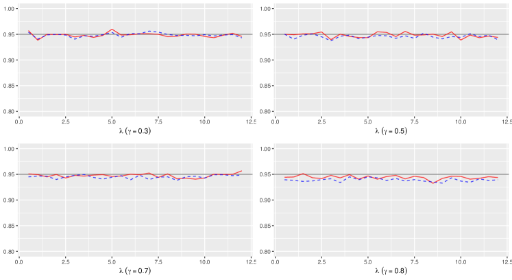
Figure 1: Empirical coverage for $\gamma$ of the positive stable distribution (nominal level 0.95). Dashed blue line ($n=100$). Solid red line ($n=200$).

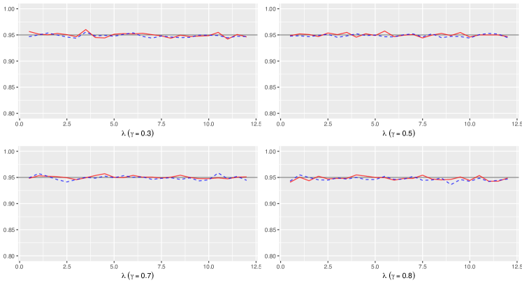
Figure 2: Empirical coverage for $\lambda$ of the positive stable distribution (nominal level 0.95). Dashed blue line ($n=100$). Solid red line ($n=200$).

Concerning the GOF, both the testing procedures based on (13) and (14) are evaluated in terms of the actual significance and power levels. To evaluate the actual significance of the two tests, independent Monte Carlo samples were generated under the null hypothesis $H_{0}$, which represents the functional hypothesis that the target r.v. is distributed according to the positive stable distribution or the Tweedie distribution. The random variate generation was carried out by considering the stochastic representations discussed in Devroye and James, (2014) and Barabesi et al., 2016b .

First, we obtained the empirical actual significance level of (13) under the positive stable model for various representative parameter choices. The results are reported as percentage of rejections at nominal level equal to $0.05$ for $n=100,200,300$ (see Table 3). The significance level was also depicted in Figure 3 for varying $\lambda$ by assuming $\gamma=0.3,0.5,0.7,0.8$ and for $n=100,200$. From Table 3 and Figure 3, it is apparent that the test shows a satisfactory actual significance level, approaching the nominal level as $n$ increases, albeit it is slightly conservative for small $\gamma$ when the sample size is small.

Table 3: Percentage values of the empirical significance level (nominal level fixed to 0.05) of the positive stable GOF test (13) for some parameter choices.

Model	$T_{100}$	$T_{200}$	$T_{300}$
$\mathrm{PS}(0.3,2)$	2.83	3.94	4.14
$\mathrm{PS}(0.4,5)$	3.49	3.89	4.34
$\mathrm{PS}(0.5,15)$	3.69	4.74	5.20
$\mathrm{PS}(0.6,20)$	3.97	4.54	4.89

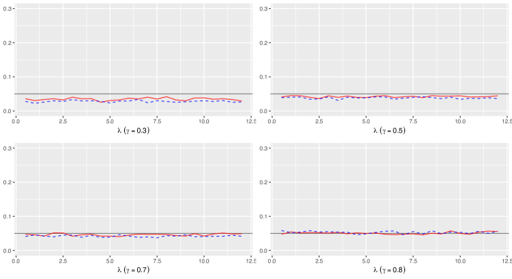
Figure 3: Empirical significance level (nominal level fixed to 0.05) with $n=100$ (dashed line) and $n=200$ (solid line).

Subsequently, we computed the empirical actual significance level of (14) under the Tweedie model for some parameter choices under both the alternative parameterization (15) and the standard one (see Table 7 for the correspondence between the parameter values). The results are reported as percentage of rejections at nominal level $0.05$ for $n=300,500,1000,1500$ (see Table 4). As it could be expected, the testing problem is much more challenging for the Tweedie GOF test owing to the additional parameter. Indeed, the test achieves the nominal level for a larger sample size such as $n=1500$. Anyway, it should be remarked that the test is conservative.

Table 4: Percentage values of the empirical significance level (nominal level fixed to 0.05) of the Tweedie GOF test (14) for some parameter choices.

Model	$\widetilde{T}_{300}^{\prime}$	$\widetilde{T}_{500}^{\prime}$	$\widetilde{T}_{1000}^{\prime}$	$\widetilde{T}_{1500}^{\prime}$
$\mathrm{TW}_{0}(0.75,0.5,0.1)$	1.17	2.11	3.31	3.43
$\mathrm{TW}_{0}(1,1,0.1)$	1.17	2.43	3.14	3.49
$\mathrm{TW}_{0}(1,1.25,0.2)$	1.09	2.03	2.66	3.20
$\mathrm{TW}(0.5,2,0.5)$	1.06	1.83	3.77	3.80
$\mathrm{TW}(0.6,2.5,0.6)$	0.17	1.49	3.26	3.40

As to the power of the two tests, we considered as alternative distributions the Linnik law denoted by $\mathrm{LI}(\gamma,\lambda,\delta)$, the shape-scale Pareto law denoted by $\mathrm{PA}(\alpha,\beta)$ with density function $f(x)=\alpha\beta^{\alpha}/x^{\alpha+1}\mathbf{1}_{\{x\geq\beta\}}$, and the shape-scale Weibull law denoted by $\mathrm{WE}(k,\lambda)$ with density function $f(x)=(k/\lambda)(x/\lambda)^{k-1}\exp(-(x/\lambda)^{k})$. Moreover, we considered the log-normal law denoted by $\mathrm{LN}(\mu,\sigma)$ and, as a further alternative, $\mathrm{LN}^{1/2}(\mu,\sigma)$, that represent respectively the laws of the r.v.s $Y=e^{X}$ and $Y=e^{X^{2}}$, where $X$ has normal law $\mathrm{N}(\mu,\sigma)$. We also considered some zero-inflated distributions, where the third parameter represents the probability of observing a zero value. Such laws are indicated by adopting a null subscript, e.g. $\mathrm{PA}_{0}(\alpha,\beta,p)$. From Table 5, the positive stable GOF show an appreciable power for all the considered alternatives. In particular, it achieves an elevate power for the $\mathrm{PA}$ and $\mathrm{LN}^{1/2}$ distribution. In contrast $\mathrm{LI}$ is similar to $\mathrm{PS}$, justifying a smaller power. The results in Table 6 evidence that the Tweedie GOF test is consistent, even if the increase of the number of parameters leads to a more challenging testing problem in terms of type 2 error. Indeed, larger samples are necessary to achieve a power comparable to the positive stable case, even if the power is satisfactory for $n$ larger than $500$. Moreover, under zero-inflated models, the procedure achieves an increasing performance as the zero probability increases.

Table 5: Percentage values of the empirical power of the positive stable GOF test (13) for some selected alternative distributions.

Model	$T_{100}$	$T_{200}$	$T_{300}$
$\mathrm{LN}(0,1.5)$	63.80	95.66	99.69
$\mathrm{PA}(5,2)$	97.77	99.43	99.97
$\mathrm{PA}(10,2)$	99.97	100.00	99.97
$\mathrm{LI}(0.5,2,0.5)$	10.03	27.43	43.91
$\mathrm{LI}(0.5,2,0.75)$	10.51	31.51	52.14
$\mathrm{LN}^{1/2}(0,1.5)$	87.97	99.29	100.00
$\mathrm{LN}^{1/2}(0,3)$	51.09	81.57	93.11

Table 6: Percentage values of the empirical power of the Tweedie GOF test (14) for some selected alternative distributions.

Model	$\widetilde{T}_{300}^{\prime}$	$\widetilde{T}_{500}^{\prime}$	$\widetilde{T}_{1000}^{\prime}$	$\widetilde{T}_{1500}^{\prime}$
$\mathrm{LN}(0,1)$	17.66	34.60	56.31	68.91
$\mathrm{WE}(5,1)$	20.46	42.03	76.00	90.57
$\mathrm{PA}(10,2)$	15.03	26.60	52.06	61.49
$\mathrm{LN}_{0}(1,0.75,0.1)$	69.74	96.91	100.00	100.00
$\mathrm{LN}_{0}(5,1,0.1)$	27.51	58.43	93.51	99.11
$\mathrm{LN}_{0}(1,0.75,0.2)$	75.17	96.57	100.00	100.00
$\mathrm{LN}_{0}(5,1,0.2)$	77.46	98.86	100.00	100.00
$\mathrm{WE}_{0}(3,1,0.1)$	74.11	99.57	100.00	100.00
$\mathrm{WE}_{0}(5,1,0.1)$	99.83	100.00	100.00	100.00
$\mathrm{WE}_{0}(3,1,0.2)$	78.69	99.97	100.00	100.00
$\mathrm{WE}_{0}(5,1,0.2)$	93.14	100.00	100.00	100.00
$\mathrm{PA}_{0}(5,2,0.1)$	20.77	41.49	69.29	85.49
$\mathrm{PA}_{0}(5,2,0.2)$	65.26	99.37	100.00	100.00
$\mathrm{PA}_{0}(10,2,0.1)$	99.86	100.00	100.00	100.00

Table 7: Corresponding values of $(\gamma,\lambda,\theta)$ for the alternative parameterization $\mathrm{TW}_{0}(\mu,w,p)$ given in (15) for the Tweedie distribution.

Model	$\gamma$	$\lambda$	$\theta$
$\mathrm{TW}_{0}(0.75,0.5,0.1)$	-1.8689607	60.297348	5.737921
$\mathrm{TW}_{0}(1,1,0.1)$	-0.7677042	3.565768	1.767704
$\mathrm{TW}_{0}(1,1.25,0.2)$	-0.9883402	2.546270	1.590672

7 Discussion and concluding remarks

In this paper, we proposed a new general inferential approach based on the Laplace transform of a random variable, that is based on exponential random censoring. This approach is useful to derive tractable parameter estimators that are used to propose suitable GOF tests for some non-standard families of random variables. The proposed estimators and test statistics are proven to be asymptotically normal leading to computationally convenient inferential procedures. We show how exponential censoring can be used to build parameter estimators and GOF tests for the positive stable and for the Tweedie laws for which specific tests are not present in the literature. The simulation study shows that the finite-sample performance of the proposed procedure is rather satisfactory even in the three-parameter case for a moderately large sample size.

References

• Aalen, (1992) Aalen, O. O. (1992). Modelling heterogeneity in survival analysis by the compound Poisson distribution. Ann. Appl. Probab., 2:951–972.
• Baccini et al., (2016) Baccini, A., Barabesi, L., and Stracqualursi, L. (2016). Random variate generation and connected computational issues for the Poisson–Tweedie distribution. Comput. Statist., 31:729–748.
• Barabesi, (2020) Barabesi, L. (2020). The computation of the probability density and distribution functions for some families of random variables by means of the Wynn-$\rho$ accelerated Post-Widder formula. Comm. Statist. Simulation Comput., 49:1333–1351.
• (4) Barabesi, L., Cerasa, A., Cerioli, A., and Perrotta, D. (2016a). A new family of tempered distributions. Electron. J. Stat., 10:3871–3893.
• (5) Barabesi, L., Cerasa, A., Perrotta, D., and Cerioli, A. (2016b). Modeling international trade data with the Tweedie distribution for anti-fraud and policy support. European J. Oper. Res., 248:1031–1043.
• (6) Barabesi, L. and Pratelli, L. (2014a). Discussion of “On simulation and properties of the stable law” by L. Devroye and L. James. Stat. Methods Appl., 23:345–351.
• (7) Barabesi, L. and Pratelli, L. (2014b). A note on a universal random variate generator for integer-valued random variables. Stat. Comput., 24:589–596.
• Barabesi and Pratelli, (2015) Barabesi, L. and Pratelli, L. (2015). Universal methods for generating random variables with a given characteristic function. J. Stat. Comput. Simul., 85:1679–1691.
• Biane et al., (2001) Biane, P., Pitman, J., and Yor, M. (2001). Probability laws related to the Jacobi theta and Riemann zeta functions, and brownian excursions. Bull. Amer. Math. Soc., 38:435–465.
• Devroye, (2009) Devroye, L. (2009). On exact simulation algorithms for some distributions related to Jacobi theta functions. Statist. Probab. Lett., 79:2251–2259.
• Devroye and James, (2014) Devroye, L. and James, L. (2014). On simulation and properties of the stable law. Stat. Methods Appl., 23:307–343.
• (12) Di Noia, A., Barabesi, L., Marcheselli, M., Pisani, C., and Pratelli, L. (2023a). Goodness-of-fit test for count distributions with finite second moment. J. Nonparametr. Stat., 35:19–37.
• (13) Di Noia, A., Marcheselli, M., Pisani, C., and Pratelli, L. (2023b). Censoring heavy-tail count distributions for parameter estimation with an application to stable distributions. Statist. Probab. Lett., 202:109903.
• Dunn and Smyth, (2005) Dunn, P. K. and Smyth, G. K. (2005). Series evaluation of Tweedie exponential dispersion model densities. Stat. Comput., 15:267–280.
• Dunn and Smyth, (2008) Dunn, P. K. and Smyth, G. K. (2008). Evaluation of Tweedie exponential dispersion model densities by Fourier inversion. Stat. Comput., 18:73–86.
• Grabchak and Grabchak, (2016) Grabchak, M. and Grabchak, M. (2016). Tempered stable distributions. Springer.
• Hasan and Dunn, (2015) Hasan, M. M. and Dunn, P. K. (2015). Seasonal rainfall totals of australian stations can be modelled with distributions from the Tweedie family. International Journal of Climatology, 35:3093–3101.
• Hougaard, (1986) Hougaard, P. (1986). Survival models for heterogeneous populations derived from stable distributions. Biometrika, 73:387–396.
• Huillet, (2000) Huillet, T. (2000). On Linnik’s continuous-time random walks. Journal of Physics A: Mathematical and General, 33:2631–2652.
• James, (2010) James, L. F. (2010). Lamperti-type laws. Ann. Appl.Probab., 20:1303–1340.
• Jørgensen, (1987) Jørgensen, B. (1987). Exponential dispersion models. J. R. Stat. Soc. Ser. B. Stat. Methodol., 49:127–145.
• Jose et al., (2010) Jose, K. K., Uma, P., Lekshmi, V. S., and Haubold, H. J. (2010). Generalized Mittag-Leffler distributions and processes for applications in astrophysics and time series modeling. In Proceedings of the Third UN/ESA/NASA Workshop on the International Heliophysical Year 2007 and Basic Space Science: National Astronomical Observatory of Japan, pages 79–92. Springer.
• Kendall, (2004) Kendall, W. S. (2004). Taylor’s ecological power law as a consequence of scale invariant exponential dispersion models. Ecological Complexity, 1:193–209.
• Luchko, (2008) Luchko, Y. (2008). Algorithms for evaluation of the Wright function for the real arguments’ values. Fract. Calc. Appl. Anal., 11:57–75.
• Marcheselli et al., (2008) Marcheselli, M., Baccini, A., and Barabesi, L. (2008). Parameter estimation for the discrete stable family. Comm. Statist. Theory Methods, 37:815–830.
• Nolan, (2020) Nolan, J. P. (2020). Univariate Stable Distributions. Springer.
• Torricelli et al., (2022) Torricelli, L., Barabesi, L., and Cerioli, A. (2022). Tempered positive Linnik processes and their representations. Electron. J. Stat, 16:6313–6347.
• Tweedie et al., (1984) Tweedie, M. C. et al. (1984). An index which distinguishes between some important exponential families. In Statistics: Applications and new directions: Proc. Indian statistical institute golden Jubilee International conference, pages 579–604. Indian Statistical Institute.