SliM-LLM: Salience-Driven Mixed-Precision Quantization for Large Language Models

Abstract

Large language models (LLMs) achieve remarkable performance in natural language understanding but require substantial computation resources and memory footprint. Post-training quantization (PTQ) is a powerful compression technique extensively investigated for its effectiveness in reducing memory usage and improving the inference efficiency of LLMs. However, existing PTQ methods are still not ideal in terms of accuracy and efficiency, especially with below 4 bit-widths. Standard PTQ methods using group-wise quantization suffer difficulties in quantizing LLMs accurately to such low-bit, but advanced methods remaining high-precision weights element-wisely are hard to realize its theoretical hardware efficiency. This paper presents a Salience-Driven Mixed-Precision Quantization scheme for LLMs, namely SliM-LLM. The scheme exploits the salience distribution of LLM weights to determine optimal bit-width and quantizers for accurate LLM quantization, while aligning bit-width partition to quantization groups for compact memory usage and fast integer computation on hardware inference. Specifically, the proposed SliM-LLM mainly relies on two novel techniques: (1) Salience-Determined Bit Allocation utilizes the clustering characteristics of salience distribution to allocate the bit-widths of each quantization group. This increases the accuracy of quantized LLMs and maintains the inference efficiency high; (2) Salience-Weighted Quantizer Calibration optimizes the parameters of the quantizer by considering the element-wise salience within the group. This balances the maintenance of salient information and minimization of errors. Comprehensive experiments show that SliM-LLM significantly improves the accuracy of various LLMs at ultra-low 2-3 bits, e.g., 2-bit LLaMA-7B achieves a 5.5-times memory-saving compared to the original model on NVIDIA A800 GPUs, and 48% decrease of perplexity compared to the state-of-the-art gradient-free PTQ method. Moreover, SliM-LLM⁺, which is integrated from the extension of SliM-LLM with gradient-based quantizers, further reduces perplexity by 35.1%. We highlight that the structurally quantized features of SliM-LLM exhibit remarkable versatility and promote improvements in the accuracy of quantized LLMs while keeping inference efficiency on hardware. Our code is available at https://github.com/Aaronhuang-778/SliM-LLM.

1 Introduction

Large language models (LLMs) have exhibited exceptional performance across a wide array of natural language benchmarks [3, 48, 19, 2]. Notably, LLaMA [41] and GPT [3] series have significantly contributed to the ongoing evolution of LLMs towards universal language intelligence. The powerful language understanding capabilities of LLMs have been transferred to multi-modal domains [25, 1, 40, 50], laying the foundation for artificial general intelligence [4]. Despite these significant achievements, the substantial computational and memory requirements of LLMs pose efficiency challenges for real-world applications and deployments, particularly in resource-constrained environments. For example, the latest LLaMA-3-70B model, with its 70 billion parameters, requires over 150GB of storage and a minimum of two NVIDIA A800 GPUs, each with 80GB of memory, for inference [21].

To reduce the computation burden, post-training quantization (PTQ), as an efficient and effective compression approach [11], has also been explored and proven successful in quantizing the weights of pre-trained LLMs [16, 20, 26, 38, 23, 6]. Faced with the dilemma of scaled-up LLMs and the limited computation resources, there is an urgent need for more aggressive compression [20, 43]. However, despite considerable efforts, significant performance degradation still occurs in low bit-width scenarios ($\leqslant$ 3-bit). To maintain the performance, unstructured mixed-precision quantization schemes [37, 20, 12] or specialized transformation computations [6, 43, 13, 7] are necessary. Yet, these approaches impose additional burdens on hardware during the inference of quantized LLMs, suffering memory overhead of element-wise bit-maps and computation overhead of codebook decoding and bit-map addressing (even preventing efficient integer computation). Moreover, even though fine-tuning can improve the accuracy of quantized LLMs, it increases the overfitting risk and requires expensive computation resources and a long time [26, 5]. Consequently, ensuring the accuracy of LLMs while maintaining efficiency during deployment remains a significant challenge for current PTQ approaches.

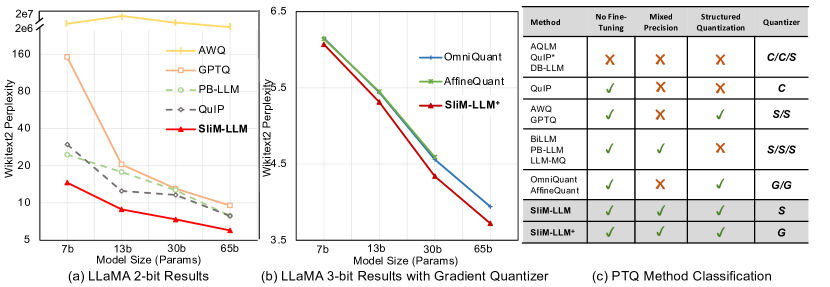
Figure 1: (a) The perplexity ($\downarrow$) of existing low-bit PTQ methods of LLaMA at 2-bit. Solid-line indicates structured quantization methods. (b) Compare PTQ methods with gradient quantizer at 3-bit. (c) Features of current low-bit quantization methods. C denotes codebook-based, S is statistic-based, and G represents gradient-based quantizers.

This paper presents the Salience-Driven Mixed-Precision LLM (SliM-LLM) framework, an accurate and hardware-efficient PTQ method for LLMs ($\leqslant$ 3-bit). SliM-LLM can be seamlessly integrated into existing advanced PTQ pipelines [16, 38], as a plug-and-play approach with mixed-precision computing for improved performance (Fig. 1). Our approach builds on the observation that not all parameters are equally important [12, 20, 37]. Specifically, a subset of salient weights significantly influences an LLM’s capabilities and tends to be concentrated in specific channels. During structured group-wise quantization, the uneven distribution of these salient channels leads to differential importance across various groups. Based on this finding, we design a structured mixed-precision quantization approach for LLMs. First, we develop a novel Salience-Determined Bit Allocation (SBA) method to allocate the optimal bit-width configuration for each structured group based on the salience distribution, minimizing the weight output relative entropy. By implementing bit-width compensation constraints, SBA maintains the average bit-width, while improving the low-bit performance. Next, we introduce the Salience-Weighted Quantizer Calibration (SQC), which amplifies the awareness of locally salient weights, preventing the degradation of sensitive information within groups. SQC works collaboratively with SBA, exploiting the local and global salience of weights to preserve the performance of LLMs after quantization. Notably, SliM-LLM does not rely on fine-tuning processes, efficiently deploying weight quantization on various LLMs. Moreover, compared to the unstructured mixed-precision methods [37, 12, 20], SliM-LLM incurs no additional bits and computation overhead. We also deploy SliM-LLM on the application-level inference tool  for LLMs, facilitating mixed-precision inference on graphics processing units (GPUs) with high performance.

Experiments show that for various LLM families, SliM-LLM surpasses existing PTQ methods on diverse benchmarks as a plug-and-play unit, particularly in low-bit scenarios. Using GPTQ as the backbone, SliM-LLM improves the perplexity scores of 2-bit LLaMA-13B and LLaMA2-13B on WikiText2 [30] from 20.44 and 28.14 to 8.87 and 9.41, denoting performance improvements of over 56%, respectively. SliM-LLM even outperforms other unstructured mixed-precision PTQ methods, such as PB-LLM [37], APTQ [18] and LLM-MQ [24], in a deployment-friendly manner, showcasing its superior low-bit accuracy and efficiency. Moreover, we integrate SliM-LLM into OmniQuant [38] and obtain SliM-LLM⁺ through gradient optimization to further improve quantization quality.

2 Related Work

Large Language Models (LLMs) have been significantly developed in diverse natural language processing domains, establishing a prominent paradigm in these fields [4, 5, 51, 3, 41]. Nevertheless, the exceptional success of LLMs depends on massive parameters and computations, posing significant challenges for deployment in resource-constrained environments. Consequently, research into the compression of LLMs has emerged as a promising field. Existing compression techniques for LLMs primarily include low-bit quantization, pruning, distillation, and low-rank decomposition [46, 17, 16, 44, 38, 6, 52, 15, 20, 33, 7]. Among these technologies, low-bit quantization gains remarkable attention, for efficiently reducing the model size without change of network structure[52, 51, 5].

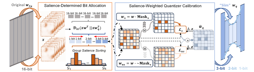
Figure 2: Illustration of our proposed SliM-LLM. The Salience-Determined Bit Allocation (SBA) optimizes activation-aware structured precision, optimizing the global information distribution in quantization. Salience-Weighted Quantizer Calibration (SQC) detects discretely distributed salient weights, enhancing the local important information in LLMs.

Quantization of LLMs can be generally divided into quantization-aware training (QAT) [27] and post-training quantization (PTQ) [44, 16, 38]. QAT, by employing a retraining strategy based on quantized perception, better preserves the performance of quantized models. LLM-QAT [27] addresses the data obstacle issue in QAT through data-free distillation. However, for LLMs with huge size of parameters, the cost of retraining is extremely inefficient[5]. Therefore, PTQ has become a more efficient choice for LLMs. For instance, LLM.int8() [27] and ZeroQuant [47] explore the quantization strategies for LLMs in block-wise, which is a low-cost grouping approach that reduces hardware burden. Smoothquant [44] scales weight and activation to decrease the difficulty of quantization. Subsequently, AWQ [26] and OWQ [23] also propose scaling transformations on outlier channels of weight to preserve their information representation capacity. GPTQ [16] reduces the group quantization error of LLMs through Hessian-based error compensation [14], achieving commendable quantization performance at 3-bit. OmniQuant [38] introduces a learnable scaling quantizer to reduce quantization errors in an output-aware manner. To enhance the accuracy of LLMs at 3-bit, APTQ [18] allocates different bit-width to different transformer blocks based on Hessian-trace, enhancing the accuracy of LLMs 3-bit. To achieve LLM quantization at ultra-low bit-width, recent novel efforts such as QuIP [6], QuIP# [43], and AQLM [13] promote quantization performance at 2-bit through learnable codebooks or additional fine-tuning. Meanwhile, approaches like SpQR[12], PB-LLM [37], and BiLLM [20] employ finer-grained partitioning for grouped quantization with unstructured mixed-precision for weights, further improving the PTQ performance. However, existing low-bit methods still rely on special structures and fine-grained grouping to ensure accuracy, which increases the difficulty of hardware deployment. Additionally, the extra fine-tuning training may pose a risk of domain-specific overfitting and undermine the efficiency of PTQ [26].

3 SliM-LLM

This section introduces a mixed-precision quantization technique called SliM-LLM, designed to overcome the performance and inference efficiency bottlenecks in mixed-precision frameworks. To address these challenges, we devise two novel strategies for LLMs, including the use of Salience-Determined Bit Allocation (SBA) based on global salience distribution to determine group bit-widths, and Salience-Weighted Quantizer Calibration (SQC) to enhance the perception of locally important weight information. We introduce SBA and SQC in Sec. 3.2 and Sec. 3.3, respectively.

3.1 Preliminaries

Quantization Framework. We first present the general uniform quantization process of LLMs according to common practice [27, 38, 1]. The quantization process requires mapping float-point weights distributed within the interval $[w_{\mathrm{min}},w_{\mathrm{max}}]$ to an integer range of $2^{N}$, where $N$ is the target bit-width. The quantization function for weight $\boldsymbol{w}_{f}\in\mathbb{R}^{n\times m}$ follows:

$$\vspace{-0.8pt}\hat{\boldsymbol{w}}_{q}=\operatorname{clamp}(\lfloor\frac{\boldsymbol{w}_{f}}{\Delta}\rceil+z,0,2^{N}-1),~{}\Delta=\frac{w_{\mathrm{max}}-w_{\mathrm{min}}}{2^{N}-1},~{}z=-\lfloor\frac{w_{\mathrm{min}}}{\Delta}\rceil\vspace{-0.8pt}$$ (1)

where $\hat{\boldsymbol{w}}_{q}$ indicates quantized weight which is integer, $\lfloor\cdot\rceil$ is round operation and $\operatorname{clamp}(\cdot)$ constrains the value within integer range (e.g. $[0,1,2,3]$, $N=2$). $\Delta$ is scale factor and $z$ is quantization zero point, respectively. When converted to 1-bit quantization, the calculation follows:

$$\hat{\boldsymbol{w}}_{b}=\operatorname{sign}(\boldsymbol{w}_{f}),~{}\operatorname{sign}(w)=\begin{cases}1&\text{if $w\geq 0$},\\ -1&\text{others}.\end{cases},~{}\alpha=\frac{1}{l}||\boldsymbol{w}_{f}||_{\ell 1}$$ (2)

where $\hat{\boldsymbol{w}}_{b}$ is binary result. $\alpha$ denots binarization scales and $l$ is the number of elements in weight [34]. We can formalize the per-layer loss in PTQ, following the common practice [31, 16]:

$$\mathcal{L}(\hat{\boldsymbol{w}}_{f})=||\boldsymbol{x}\boldsymbol{w}_{f}^{\top}-\boldsymbol{x}\hat{\boldsymbol{w}}_{f}^{\top}||^{2}=\operatorname{tr}((\hat{\boldsymbol{w}}_{f}-\boldsymbol{w})\boldsymbol{H}(\hat{\boldsymbol{w}}_{f}-\boldsymbol{w})^{\top})$$ (3)

where $\boldsymbol{x}\in\mathbb{R}^{t\times m}$ denotes the input vectors from calibration dataset, $\hat{\boldsymbol{w}}_{f}\in\mathbb{R}^{n\times m}$ is dequantized weight from quantization result in Eq. (1) or Eq. (2), and $\boldsymbol{H}=\frac{1}{P}\sum_{k=1}^{P}\boldsymbol{x}^{[k]}\boldsymbol{x}^{[k]\top}$ is proxy Hessian matrix by Levenberg-Marquardt approximation [29, 14] from a set of input activations.

Parameter Salience. In LLMs, the importance of each individual element in weight matrix is various [12, 15]. According to Eq. (3), the impact of quantizing a single element on the model’s output loss differs. Elements that significantly influence the loss are termed salient weights. Consequently, we follow the SparseGPT [15] to define the salience of each element as:

Definition 1.

In the quadratic approximation of the loss as expressed in Eq. (3), we give the Hessian matrix $H\in\mathbb{R}^{m\times m}$ generated by $\frac{1}{P}\sum_{k=1}^{P}\boldsymbol{x}^{[k]}\boldsymbol{x}^{[k]^{\top}}$ for a weight matrix, the removal of the element at $(i,j)$ induces an error $\delta_{i,j}=\frac{w_{i,j}^{2}}{[\boldsymbol{H}^{-1}]_{j,j}^{2}}$ to the output matrix for linear projection in LLMs.

where $[\boldsymbol{H}^{-1}]_{jj}$ denotes the $j^{th}$ diagonal entry for the inverse Hessian, and $\boldsymbol{H}^{-1}$ can be efficiently calculated through Cholesky decomposition [22]. According to Definition. 1, we map the elimination error $\delta_{ij}$ to the salience measure of each weight element in LLMs, representing the impact of different weights on the output loss and the language capabilities, which also leads the generation of mixed-precision quantization strategies [12, 37, 20, 24] for LLMs. However, existing mixed-precision solutions require the discrete allocation of bit-widths across the entire weight matrix, which imposes a significant burden on hardware computations, thereby affecting the inference efficiency.

3.2 Salience-Determined Bit Allocation

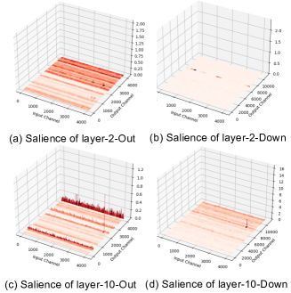
Figure 3: Salience in LLaMA-7B.

In the following, we reveal phenomenon of spatial clustering in the distribution of weight salience, which inspires our proposed concept of structured mixed-precision quantization for LLMs, and then present the Salience-Determined Bit Allocation (SBA) technique to optimize bit-width allocation.

3.2.1 Spatial Clustering of Global Salience

We first conduct an empirical investigation into the weight salience distribution. The results reveal that certain channels exhibit higher salience and show tendencies for spatial clustering. As illustrated in Fig. 3, salient clustering are identified around the $2100^{th}$, $3218^{th}$ and $3853^{rd}$ channels within the $2^{nd}$ layer’s attention projection of the LLaMA-7B model. A similar structured pattern is observed near the $600^{th}$, $2200^{th}$ and $3992^{nd}$ channels in the $10^{th}$ layer. Also, clustered salience is detected in other layers (as shown in Fig. 3). More examples of spatial clustering of salience are provided in Appendix F.

Then, we analyze the underlying causes of this phenomenon from a theoretical perspective. According to Definition 1, the salience of weights in LLMs can be quantified numerically by the weight magnitudes and the diagonal elements of the Hessian matrix, which is further approximated by the product of input activations $\boldsymbol{x}\boldsymbol{x}^{\top}$. In LLMs, activations exhibit more extreme outliers, while the numerical differences in weights are relatively slight [44, 32]. Therefore, we propose an analysis of how outlier values in input activations influence the distribution of weight salience:

Theorem 1.

Given the input calibration activation $\boldsymbol{x}\in\mathbb{R}^{t\times m}$ with an outlier value $x_{p,q}^{*}\gg x_{i,j},\forall i\in[0,t],i\neq p,\forall j\in[0,m],j\neq q$ at the position of token-$p$ and channel-$q$. The diagonal elements of $\boldsymbol{x}\boldsymbol{x}^{\top}$ also shows outlier value at $[\boldsymbol{x}\boldsymbol{x}^{\top}]_{p,p}$, as ${x_{p,q}^{*}}^{2}$ produced by $[\boldsymbol{x}\boldsymbol{x}^{\top}]_{i,i}=\sum_{k=1}^{n}x_{i,k}^{2}$ only appearing at position $(p,p)$, which further leads to the parameter salience larger at the $p^{th}$ channel of weight, where $\delta_{:,p}>\delta_{:,k},\delta_{:,k}=\frac{w_{:,k}^{2}}{[\boldsymbol{H}^{-1}]_{k,k}^{2}},\forall k\in[0,t],k\neq p$.

Theorem 1 elucidates the impact of outlier tokens on the channel-wise distribution of weight salience (detailed proof is provided in Appendix F.1). Additionally, recent studies [32, 45] indicate that outlier tokens in LLMs activations tend to cluster regionally at specific locations, resulting in sequences of consecutive significant tokens. According to Theorem 1, these consecutive tokens will lead to channel clustering results of weight salience, as evidenced by the consecutive salient channels shown in Fig. 3. This also means that when we divide the weight into multiple groups with continuous channels, the overall salience of different groups is different.

Due to the unstructured mixed-precision, which involves additional storage requirements and inference operations, the computational format is not deployment-friendly. However, the spatial clustering of weight salience observed in this section strongly inspired the development of structured mixed-precision strategies with flexible bit-widths while maintaining inference efficiency. Therefore, we aim to allocate bit-width structurally based on group-wise salience differences. This approach not only enhances quantization accuracy but also ensures the deployment efficiency of LLMs.

3.2.2 Salience-Determined Bit Allocation for Structured Group

To allocate optimal bit-widths to each group, we introduce a Salience-Determined Bit Allocation (SBA) technique for mixed-precision LLMs, as depicted in Fig. 1. This technique, predicated on the differences in group salience, determines the optimal bit-width allocation for different groups by minimizing the distance of information entropy with the original weight output.

Specifically, we first utilize the average salience as the importance indicator for each weight group and rank them accordingly. The proposed SBA optimizes the following formula to determine the optimal number of salient-unsalient quantization groups of LLMs:

$$\begin{aligned} \text{Objective}:&\mathop{\mathrm{argmin}}\limits_{g_{1},...g_{n}}\mathcal{D}_{kl}~{}(\boldsymbol{x}\boldsymbol{w}_{f}^{\top}||\boldsymbol{x}\mathcal{Q}(\boldsymbol{w}_{f}|[g_{1},...g_{n}])^{\top}),\\ \text{Constrain}:&|\mathcal{G}_{N-1}|=|\mathcal{G}_{N+1}|,~{}\mathcal{G}_{N-1}=\{g_{i}|g_{i}=N-1\},~{}\mathcal{G}_{N+1}=\{g_{j}|g_{j}=N+1\},\end{aligned}$$ (4)

where $\mathcal{D}_{kl}(\cdot||\cdot)$ denotes the Kullback-Leibler (KL) divergence between two outputs, $N$ is the targeted average bit-width. $\mathcal{Q}$ generally represents the quantization and de-quantization processes, employing group-wise mixed precision designated as $[g_{1},...g_{k}]$, where $g_{i}$ represents the bit-width for the $i^{th}$ group and $\mathcal{G}$ is a set of groups with the same bit-width. We apply a compensation constraints strategy to maintain a consistent average bit-width for our SBA. For example, in 2-bit quantization, the groups with the highest salience are quantized to 3-bit. To offset the additional bits, we quantize an equal number of groups with the lowest salience to 1-bit, while the remaining groups are set to 2-bit.

We utilize an effective double-pointer search (more detailed examples in Appendix C) to optimize our objective in Eq. (4). When the weight output channel size is $m$ and group size is $128$, $k=\frac{m}{128}$, the search region for weight is limited to $[0,\frac{k}{2}]$, which is highly efficient with limited searching space, e.g., only 16 iterations are needed in LLaMA-7B. We also provide detailed searching error examples in Appendix C. Notably, SBA diverges from traditional quantization with mean squared error (MSE) in Eq. (3) by instead utilizing the KL divergence as its measure of loss. Beyond simply reducing numerical quantization errors, SBA leverages relative entropy as a mixed bit-width metric, aiming to maximize the mutual information [35] between the quantized and original weights of the LLMs. This approach enhances the model’s capacity for information representation under lower bit quantization.

3.3 Salience-Weighted Quantizer Calibration

In addition to the global group-wise distribution of salience, we notice that salience within the group still shows local differences in discrete distribution. Common existing quantizers apply uniform consideration across all weights to minimize the effect (error) of quantization, lacking the capability to perceive differences in local salience. Therefore, in this section, we introduce a Salience-Weighted Quantizer Calibration (SQC) to enhance the information of significant weights within the group by amplifying the quantizer awareness of salient weight.

3.3.1 Discrete Distribution of Local Salience

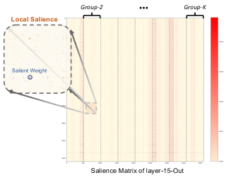
Figure 4: Local salience distribution of the $10^{th}$ MHA output layer in LLaMA-7B.

In the aforementioned section, we allocate the bit-width for each group based on the global salience. However, the salience among different elements within the same group still locally exhibits an unstructured difference. Specifically, as depicted in the salience distribution in Fig. 4, within the $10^{th}$ attention output layer of LLaMA-7b, a subset of sparse weights within the comparatively less salient Group-2 still maintains a high level of importance. In LLMs, a small number of weights with outliers may affect the distribution of salience in an unstructured manner, as described in Definition 1. These discrete weights typically account for only approximately 1% of the total weights within the group but play a crucial role in the modeling capability of LLMs.

The existing vanilla quantizers still face the challenge in representing significant weight information, for only considering mean error of all elements within a group. When quantizing weights according to Eq. (1) in group-wise format, a large number of relatively non-salient weights at the intra-group statistical level tend to dominate the parameters generated by the quantizer. This leads to a degradation of salient information within the group, thereby affecting the model performance of LLMs.

3.3.2 Salience-Weighted Quantizer Calibration for Local Salience Awareness

To prevent the degradation of local salient weight information in each group, we propose the Salience-Weighted Quantizer Calibration (SQC), which enhances the expression of salient weights through locally unstructured salience awareness, thereby reducing the quantization error of these significant elements and improving the compressed performance of LLMs. SQC first introduces the calibration parameter $\gamma$ to the quantizer, liberating the perception interval during quantization:

$$\Delta=\frac{\gamma(w_{\mathrm{max}}-w_{\mathrm{min}})}{2^{N}-1},~{}z=-\lfloor\frac{\gamma w_{\mathrm{min}}}{\Delta}\rceil$$ (5)

where $\gamma$ expands the solution space of the quantizer, subsequently minimizes the loss of quantization in the salience-weighted objective:

$$\mathop{\mathrm{argmin}}\limits_{\gamma}~{}\mathcal{L}_{s}(\boldsymbol{w}_{s},\operatorname{dequant}(\hat{\boldsymbol{w}}_{sq},\Delta,z))+\mathcal{L}_{u}(\boldsymbol{w}_{u},\operatorname{dequant}(\hat{\boldsymbol{w}}_{uq},\Delta,z))$$ (6)

where $\mathcal{L}$ represents the ${\ell_{2}}$ loss, aligned with Eq. (3). $\boldsymbol{w}_{s}$ and $\boldsymbol{w}_{u}$ denotes the salient weights and less salient part, respectively, generated from a mask operation, $\hat{\boldsymbol{w}}_{sq}$ and $\hat{\boldsymbol{w}}_{uq}$ are quantized results. Based on a common observation [12, 37, 20], the proportion of relatively salient weights in each group is only 1-5%. Therefore, we employ the 3-$\sigma$ rule to mask groups based on the salience distribution to select the unstructured salience part. In Eq. (6), $\gamma$ flexibly adjusts $\Delta$ and $z$ to search the optimal loss under $\gamma^{*}$, without bringing additional parameters, as $\boldsymbol{w}_{s}$ and $\boldsymbol{w}_{s}$ share the same quantizer. The search space for $\gamma$ by linearly dividing the interval [1-$\lambda$, 1+$\lambda$] into 2$n$ candidates. We empirically set $\lambda$ at 0.1 and $n$ at 50 to achieve a balance between efficiency and accuracy.

SQC effectively mitigates the degradation of local salient weights within groups (more evidence is provided in Appendix D). Additionally, SQC only requires the optimization of $\gamma$ during quantization and without distinguishing unstructured parts in storage and inference stages, thereby avoiding hardware overhead. Combined with SBA, they jointly enhance the awareness of local and global salient weights, capturing significant information in LLMs to improve quantization performance.

Table 1: Quantization results of LLaMA family with statistic quantizer. We report the WikiText2 perplexity in this table, C4 results are shown in Appendix G.

#W PPL$\downarrow$	Method	1-7B	1-13B	1-30B	1-65B	2-7B	2-13B	2-70B	3-8B	3-70B
16-bit	-	5.68	5.09	4.10	3.53	5.47	4.88	3.31	5.75	2.9
3-bit	APTQ	6.76	-	-	-	-	-	-	-	-
	LLM-MQ	-	-	-	-	-	8.54	-	-	-
	RTN	7.01	5.88	4.87	4.24	6.66	5.51	3.97	27.91	11.84
	AWQ	6.46	5.51	4.63	3.99	6.24	5.32	-	8.22	4.81
	GPTQ	6.55	5.62	4.80	4.17	6.29	5.42	3.85	8.19	5.22
	SliM-LLM	6.40	5.48	4.61	3.99	6.24	5.26	3.67	7.16	4.08
2-bit	LLM-MQ	-	-	-	-	-	12.17	-	-	-
	RTN	1.9e3	781.20	68.04	15.08	4.2e3	122.08	27.27	1.9e3	4.6e5
	AWQ	2.6e5	2.8e5	2.4e5	7.4e4	2.2e5	1.2e5	-	1.7e6	1.7e6
	GPTQ	152.31	20.44	13.01	9.51	60.45	28.14	8.78	210.00	11.90
	QuIP	29.74	12.48	11.57	7.83	39.73	13.48	6.64	84.97	13.03
	PB-LLM	24.61	17.73	12.65	7.85	25.37	49.81	NAN	44.12	11.68
	SliM-LLM	14.58	8.87	7.33	5.90	16.01	9.41	6.28	39.66	9.46

3.4 Implementation Pipeline of SliM-LLM

We integrate our mixed-precision framework into advanced PTQ methods, such as GPTQ [16] and OmniQuant [38], all of which are deployment-friendly with group-wise quantization. We primarily integrate SBA and SQC into GPTQ to get SliM-LLM. For SliM-LLM⁺, the SBA is plugged into OmniQuant with a learnable quantizer. The complete pipeline of SliM-LLM is provided in Algorithm 1, and a more detailed implementation is listed in Appendix B.1.

Algorithm 1 Main Framework of SliM-LLM.

func $\operatorname{SliM-LLM}$($\boldsymbol{w}$, $\boldsymbol{x}_{F}$, $\beta$, $\lambda$, $N$)
Input: $\boldsymbol{w}\in\mathbb{R}^{n\times m}$ - FP16 weight
          $\boldsymbol{x}_{F}\in\mathbb{R}^{t\times m}$ - calibration data
          $\beta$ - group size
          $\lambda$ - hessian regularizer
          $N$ - average bit-width
Output: $\hat{\boldsymbol{w}}_{q}$ - quantized weight

1:  $\boldsymbol{H}\coloneqq\frac{1}{P}\sum_{k=1}^{P}\boldsymbol{x}_{F}^{[k]}\boldsymbol{x}_{F}^{[k]T}$ hessian matrix

2:  $\boldsymbol{H}^{\mathrm{in}}\coloneqq$ Cholesky$({(\boldsymbol{H}+\lambda\boldsymbol{I})}^{-1})$

3:  $\hat{\boldsymbol{w}}_{q}\coloneqq 0^{n\times m}$

4:  $\mathcal{G}\{\cdot\}\coloneqq\operatorname{SBA}(\boldsymbol{w},\boldsymbol{x}_{F},\boldsymbol{H}^{\mathrm{in}},\beta,N)$

5:  for $b=0,\beta,2\beta,...$ do

6:     $\boldsymbol{w}^{b}\coloneqq\boldsymbol{w}_{:,b:b+\beta}$

7:     $g_{b}\coloneqq\mathcal{G}[b]$

8:     $\boldsymbol{w}^{b}_{s},\boldsymbol{w}^{b}_{us}\coloneqq\operatorname{sal\_mask}(\boldsymbol{w}^{b})$

9:     $\hat{\boldsymbol{w}}_{q}^{b}\coloneqq\operatorname{SQC}(\boldsymbol{w}^{b}_{s},\boldsymbol{w}^{b}_{us},g_{b})$

10:     GPTQ-error compensation:

11:     $\boldsymbol{E}\coloneqq(\boldsymbol{w}_{:,b:b+\beta}-\hat{\boldsymbol{w}}_{q}^{b})/\boldsymbol{H}^{\mathrm{in}}_{bb:b+\beta b+\beta}$

12:     $\boldsymbol{w}_{:,b+\beta:}\coloneqq\boldsymbol{w}_{:,b+\beta:}-\boldsymbol{E}\cdot\boldsymbol{H}^{\mathrm{in}}_{b:b+\beta,b+\beta:}\$

13:  end for

14:  return $\hat{\boldsymbol{w}}_{q}$

4 Experiments

We evaluated SliM-LLM and SliM-LLM⁺ under weight-only conditions, focusing on 2/3-bit precisions. Per-channel group quantization is utilized in our framework with 128 set as group size in experiments. Since no back-propagation in SliM-LLM, the quantization is carried out on a single NVIDIA A800 GPU. For SliM-LLM⁺, we employ the AdamW optimizer, following OmniQuant [38], which is also feasible on a single A800. We randomly select 128 samples from WikiText2 [30] as calibration data, each with 2048 tokens.

Models and Evaluation. To comprehensively demonstrate the low-bit performance advantages of SliM-LLM and SliM-LLM⁺, we conduct experiments across OPT [49], LLaMA [41], LLaMA-2 [42] and LLaMA-3¹. We employ the perplexity as our evaluation metric, which is widely recognized as a stable measure of language generation capabilities [16, 26, 20, 37, 38, 6, 13, 21], particularly in compression scenarios. Experiments are carried out on the WikiText2 [30] and C4 [36]datasets. Furthermore, to assess the practical application capabilities of quantized LLMs, we also evaluate their accuracy on zero-shot benchmarks, including PIQA [2], ARC [10], BoolQ [9], and HellaSwag [10].

Baseline. Since SliM-LLM and SliM-LLM⁺ are efficient PTQ approaches without additional training or fine-tuning, QAT and re-training methods are not within the comparison range of our work. The experiments evaluate existing advanced quantization methods and GPU-friendly computations, including vanilla round-to-nearest (RTN), GPTQ [16], AWQ [26]. And mixed-precision quantization techniques, including PB-LLM [37] ($\frac{1}{7}\times 8$-bit+$\frac{6}{7}\times 1$-bit), LLM-MQ [24], and APTQ [18], as well as the codebook-based method QuIP [6] are also compared in this work. We compare SliM-LLM⁺ with gradient optimizer-based methods such as OmniQuant [38] and AffineQuant [28].

4.1 Main Results.

We show experiments within the LLaMA family in this section and detailed results for the OPT models are available in Appendix G. For language generation tasks, as depicted in Tab. 1, SliM-LLM markedly outperforms its backbone GPTQ, particularly under the 2-bit. Specifically, on LLaMA-7B, SliM-LLM achieves a 90% decrease in perplexity, while on LLaMA-3-8B, it improves performance by 81%. In comparison with the unstructured mixed-precision PB-LLM and the codebook-based QuIP method, SliM-LLM further reduces the perplexity by 41%~51%. As shown in Tab. 1, the performance of SliM-LLM⁺ is still ahead compared to OmniQuant and AffineQuant, further proving the effectiveness and of the mixed-precision framework proposed in our work. We also provide dialogue examples of 2-bit instruction fine-tuning Vicuna-13B [8] and LLaMA-13B in Appeandix H.

Morever, our method exhibits zero-shot advantages at 2-bit, as shown in Tab. 3, where SliM-LLM and SliM-LLM⁺ still outperforms other methods. For instance, compared with GPTQ and OmniQuant, our approach achieves an average improvement of 4.19% and 1.91% on LLaMA-7B. Meanwhile, for LLaMA-65B, 2-bit SliM-LLM and SliM-LLM⁺ is close to FP16 results (less than 6% degradaion in accuracy). Overall, our proposed mixed-precision framwork demonstrates superior performance across different model sizes, with its advantages becoming increasingly significant at lower bit-width.

Table 2: Quantization results of LLaMA-1 and LLaMA-2 models with learnable quantizer. We report the WikiText2 perplexity in this Table, C4 results are shown in Appendix G.

#W PPL$\downarrow$	Method	1-7B	1-13B	1-30B	1-65B	2-7B	2-13B	2-70B
16-bit	-	5.68	5.09	4.10	3.53	5.47	4.88	3.31
3-bit	OmniQuant	6.15	5.44	4.56	3.94	6.03	5.28	3.78
	AffineQuant	6.14	5.45	4.59	-	6.08	5.28	-
	SliM-LLM+	6.07	5.37	4.34	3.72	5.94	5.11	3.35
2-bit	OmniQuant	9.72	7.93	7.12	5.95	11.06	8.26	6.55
	AffineQuant	13.51	7.22	6.49	-	10.87	7.64	-
	SliM-LLM+	9.68	7.17	6.41	5.74	10.87	7.59	6.44

Table 3: Performance comparisons of different quantization methods for zero-shot tasks.

Model / Acc$\uparrow$	#W	Method	PIQA	ARC-e	ARC-c	BoolQ	HellaSwag	Winogrande	Avg.
LLaMA-7B	16-bit	-	77.47	52.48	41.46	73.08	73.00	67.07	64.09
2-10	2-bit	GPTQ	55.49	31.02	22.17	53.49	33.84	41.91	39.65
	2-bit	AWQ	47.78	28.77	21.31	31.19	24.47	40.03	32.26
	2-bit	SliM-LLM	57.83	33.46	25.09	56.05	36.70	52.64	43.84
2-10	2-bit	OmniQuant	63.63	43.91	27.32	58.02	48.78	52.97	49.11
	2-bit	SliM-LLM+	64.96	45.66	28.67	64.59	48.86	53.35	51.02
LLaMA-13B	16-bit	-	79.10	59.89	44.45	68.01	76.21	70.31	66.33
2-10	2-bit	GPTQ	70.37	47.74	35.88	51.57	61.39	60.84	54.63
	2-bit	AWQ	49.23	30.01	29.49	30.88	26.72	46.30	35.44
	2-bit	SliM-LLM	73.19	47.95	36.27	55.92	63.04	61.79	56.36
2-10	2-bit	OmniQuant	73.14	49.38	36.93	63.34	62.19	61.77	57.64
	2-bit	SliM-LLM+	74.15	50.26	37.04	64.31	63.57	63.11	58.74
LLaMA-30B	16-bit	-	80.08	58.92	45.47	68.44	79.21	72.53	67.44
2-10	2-bit	GPTQ	71.92	48.27	36.20	61.27	65.76	63.11	57.76
	2-bit	AWQ	49.17	28.56	25.97	34.73	24.97	46.99	35.07
	2-bit	SliM-LLM	75.52	51.29	39.29	62.01	66.10	64.07	59.71
2-10	2-bit	OmniQuant	76.23	53.23	39.52	63.34	65.57	64.82	60.22
	2-bit	SliM-LLM+	76.31	54.07	39.79	63.35	67.14	64.93	60.91
LLaMA-65B	16-bit	-	80.79	58.71	46.24	82.29	80.72	77.50	71.04
2-10	2-bit	GPTQ	76.16	52.48	40.14	77.23	71.96	70.22	64.70
	2-bit	SliM-LLM	77.09	53.72	40.25	77.51	72.05	70.91	65.26
2-10	2-bit	OmniQuant	77.78	53.71	40.90	78.04	74.55	68.85	65.64
	2-bit	SliM-LLM+	78.06	53.90	41.18	78.33	75.59	69.99	66.18

4.2 Ablation Results.

We conduct a detailed ablation study to illustrate the benefits of bit-width allocation and the impact of each component. Fig. 5(a) compares three strategies for allocating bit-widths across groups, including random allocation, head-tail allocation by spatial order, and our proposed SBA. When the average bit-width remains constant, random and head-tail mixed-precision allocation prove ineffective and even result in performance degradation, as shown in Fig. 5(a). In contrast, SBA consistently delivers significant improvements in post-quantization performance, validating the efficacy of our mixed-precision approach. Fig. 5(b) presents the ablation effects of SBA and SQC, demonstrating that both methods, based on the perception of global and local salience, enhance quantization performance. SBA is particularly effective in smaller models, and combining these two methods can further boost capabilities of LLMs. We also provide the detailed ablation results on group size in Appendix E.

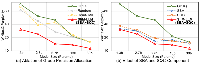
Figure 5: Ablation results on OPT models. Random means randomly selecting the same number of lower/higher-bit groups; head-tail denotes using the head groups as the lower-bit and the same number of tails as the higher-bit on the original sequence of group.

Table 4: Deployment results of GPTQ and Slim-LLM on GPU. Group size is set to 128.

#W

LLaMA-*

1-7B

1-13B

2-7B

WM

RM

PPL$\downarrow$

Token/s

WM

RM

PPL$\downarrow$

Token/s

WM

RM

PPL$\downarrow$

Token/s

FP16

-

12.6G

14.4G

5.68

69.2

24.3G

27.1G

5.09

52.5

12.7G

14.6G

5.47

69.3

3-bit

GPTQ

3.2G

5.1G

6.55

83.4

5.8G

8.7G

5.62

57.6

3.2G

5.2G

6.29

56.3

SliM-LLM

3.2G

5.2G

6.40

79.1

5.8G

8.8G

5.48

48.5

3.2G

5.4G

6.26

55.9

2-bit

GPTQ

2.2G

4.1G

152.31

83.9

4.0G

7.5G

20.44

92.6

2.2G

4.1G

60.45

83.6

SliM-LLM

2.3G

4.4G

14.58

61.2

4.1G

7.8G

8.87

73.7

2.3G

4.1G

16.01

64.4

4.3 Efficient Inference on Device

We utilize the open-source AutoGPTQ to extend CUDA kernel supporting experimental mixed-precision inference, with detailed process in Appendix B.2. We evaluate the deployment performance of LLaMA-7/13B and LLaMA-2-7B under 2/3-bit settings. The results indicate that our mixed-precision approach maintains a good compression rate on GPUs and significantly enhances model accuracy, only with a slight decrease in inference speed on the A800 (due to the inference alignment of different bit-width). Since current 1-bit operations lack well hardware support, additional consumption of storage and computation is required on device. There remains considerable scope for optimization in mixed-precision computing, and we aim to further improve this in future work.

5 Conclusion

In this work, we introduce SliM-LLM, a structured mixed-precision PTQ framework tailored for LLMs, designed to enhance performance with low-bit weights in a deployment-friendly manner. The essence of SliM-LLM lies in employing the Salience-Determined Bit Allocation to dynamically allocate bit widths, thereby improving the preservation of global salience information. Within groups, the Salience-Weighted Quantizer Calibration is designed to enhance local information perception, further minimizing the loss associated with locally salient weights. Experiments validate the effectiveness of SliM-LLM, showing notable accuracy improvements across various LLMs, and ensuring efficiency in inference. In conclusion, SliM-LLM is versatile and can be seamlessly integrated with different quantization frameworks and successfully improves the performance of LLMs supporting practical deployment in resource-constrained environments.

Appendix A Broader Impacts and Limitations

A.1 Broader Impacts

This paper introduces a mixed-precision technique to achieve accurate and efficient low-bit weight quantization for large language models (LLMs). This approach makes LLMs more efficient and accessible, potentially extending their pervasive impact. From a positive perspective, quantization makes the use of LLMs easier, benefiting a broader audience, particularly those in lower-income groups. It reduces the cost and hardware barriers to deploying LLMs and promotes edge inference of these models (mitigating the risk of privacy data breaches), contributing to societal productivity. On the downside, LLMs could be exploited by malicious users to generate and spread false information. Quantization does not prevent the inherent negative impacts of LLMs, nor does it exacerbate them.

A.2 Limitations

Though the mixed-precision framework significantly improves the quantization performance of LLMs, the current out-of-the-box deployment tools still cannot well support efficient mixed-precision computing. Meanwhile, the support for 1/2/3-bit inference on GPUs remains limited, which affects the inferencing advantages of low-bit models. We believe there is significant room for improvement in the hardware efficiency of mixed-precision LLMs in the future.

A.3 Experiments Reproducibility

Our code is included in the supplementary materials. For instructions on how to reproduce various experiments, please refer to the accompanying code scripts and algorithm description in our paper. We also provide the download and use details of the datasets mentioned in the experiment part.

Appendix B SliM-LLM Implementation

B.1 Detailed Implementation

In this section, we present the specific implementation details of SliM-LLM, which utilizes GPTQ [16] as its backbone for mixed-precision quantization and incorporates both SBA and SQC. SliM-LLM⁺ is consistent with SliM-LLM in SBA computations but does not include the SQC component, instead retaining learnable weight clipping (LWC) approach in OmniQuant [38] for gradient optimization.

Algorithm 2 Detailed functions in SliM-LLM.

func $\operatorname{SBA}(\boldsymbol{w},\boldsymbol{x}_{F},\boldsymbol{H}^{\mathrm{in}},\beta,N)$

1:  $\mathcal{G}\{\cdot\}\coloneqq\{0\}$ //  initialize group bit-width

2:  $e\coloneqq\operatorname{inf}$ //  bit-width searching error

3:  $p^{*}\coloneqq 0$ //  number of ($N$-1)-bit and ($N$+1)-bit

4:  $l\coloneqq N-1$ //  lower bit-width

5:  $h\coloneqq N+1$ //  higher bit-width

6:  $S\{\cdot\}\coloneqq\operatorname{average}(\frac{\boldsymbol{w}^{2}}{[\boldsymbol{H}^{\mathrm{in}}]_{\mathrm{diag}}^{2}})$

7:  for $p=1,2,...,[\frac{m}{2\beta}]$ do

8:     $\hat{\boldsymbol{w}}_{l}^{b}\coloneqq\operatorname{fakequant}(\boldsymbol{w}_{b\in\operatorname{top\_k\_min(p)}}^{b},l,)$

9:     $\hat{\boldsymbol{w}}_{h}^{b}\coloneqq\operatorname{fakequant}(\boldsymbol{w}_{b\in\operatorname{top\_k\_max(p)}}^{b},h,)$

10:     $\hat{\boldsymbol{w}}_{N}^{b}\coloneqq\operatorname{fakequant}(\boldsymbol{w}_{b\in\mathrm{others}}^{b},N,)$

11:     $\hat{\boldsymbol{w}}_{q}\coloneqq\hat{\boldsymbol{w}}_{l}^{b}\cup\hat{\boldsymbol{w}}_{l}^{b}\cup\hat{\boldsymbol{w}}_{h}^{b}$

12:     if $\mathcal{D}_{kl}~{}(\boldsymbol{x}\boldsymbol{w}^{\top}~{}||~{}\boldsymbol{x}\hat{\boldsymbol{w}}_{q}^{\top})<e$ then

13:        $e\coloneqq\mathcal{D}_{kl}~{}(\boldsymbol{x}\boldsymbol{w}^{\top}~{}||~{}\boldsymbol{x}\hat{\boldsymbol{w}}_{q}^{\top})$

14:        $p^{*}\coloneqq p$

15:     end if

16:  end for

17:  $\mathcal{G}\{l\}\coloneqq S\{\operatorname{top\_k\_min}(p^{*})=l\}$

18:  $\mathcal{G}\{h\}\coloneqq S\{\operatorname{top\_k\_max}(p^{*})=h\}$

19:  $\mathcal{G}\{N\}\coloneqq S\{\operatorname{middle\_k}([\frac{m}{2}]-2p^{*})=N\}$

20:  return $\mathcal{G}\{\cdot\}$

func $\operatorname{SQC}(\boldsymbol{w}^{b}_{s},\boldsymbol{w}^{b}_{us},g_{b})$

1:  $w_{\mathrm{max}}\coloneqq\operatorname{max}(\boldsymbol{w}^{b}_{s}\cup\boldsymbol{w}^{b}_{us})$

2:  $w_{\mathrm{min}}\coloneqq\operatorname{min}(\boldsymbol{w}^{b}_{s}\cup\boldsymbol{w}^{b}_{us})$

3:  $\lambda\coloneqq 0.1$

4:  $n\coloneqq 50$

5:  $e\coloneqq\operatorname{inf}$ //  scale searching error

6:  $\Delta^{*}\in\mathbb{R}^{n\times 1}$ //  per-channel scale

7:  $z^{*}\in\mathbb{R}^{n\times 1}$ //  per-channel zero point

8:  for $\gamma\in~{}[1-\lambda,1+\lambda]$ with $2n$ slices do

9:     $\Delta\coloneqq\gamma(w_{\mathrm{max}}-w_{\mathrm{min}})/(2^{g_{s}}-1)$

10:     $z\coloneqq-\lfloor(\gamma w_{\mathrm{min}})/{\Delta}\rceil$

11:     $\hat{\boldsymbol{w}}_{s}^{b}\coloneqq\operatorname{fakequant}(\boldsymbol{w}^{b}_{s},g_{b},\Delta,z)$

12:     $\hat{\boldsymbol{w}}_{us}^{b}\coloneqq\operatorname{fakequant}(\boldsymbol{w}^{b}_{us},g_{b},\Delta,z)$

13:     $\mathcal{L}_{s}\coloneq||\boldsymbol{w}_{s}^{b}-\hat{\boldsymbol{w}}_{s}^{b}||^{2}$

14:     $\mathcal{L}_{us}\coloneq||\boldsymbol{w}_{us}^{b}-\hat{\boldsymbol{w}}_{us}^{b}||^{2}$

15:     if $\mathcal{L}_{s}+\mathcal{L}_{us}<e$ then

16:        $e\coloneqq\mathcal{L}_{s}+\mathcal{L}_{us}$

17:        $z^{*}\coloneqq z$

18:        $\Delta^{*}\coloneqq\Delta$

19:     end if

20:  end for

21:  $\hat{\boldsymbol{w}}_{q}^{b}\coloneqq\operatorname{fakequant}(\boldsymbol{w}^{b},g_{b},\Delta^{*},z^{*})$

22:  return $\hat{\boldsymbol{w}}_{q}^{b}$

Algorithm 2 primarily encompasses the core details of both SBA and SQC. In SBA, the importance of each group is determined by sorting the average salience of groups, followed by a bi-pointer search that increases the number of ($N-1$)-bit and ($N+1$)-bit groups to maintain their quantity equilibrium. The optimization function then utilizes the KL divergence from Eq. (4) to determine the optimal mixed-precision ratio. SQC, on the other hand, enhances its information by amplifying the quantization error of unstructured weight groups. When the last two parameters, scale and zero point, in the $\operatorname{fakequant}(\cdot)$ function are omitted, the default values from Eq. (1) are used.

B.2 Mixed Bit Storage and Computing

We developed a framework for storage and inference deployment supporting mixed-precision quantization based on AutoGPTQ. The deployment process is as follows. After completing mixed-precision quantization with SliM-LLM, it outputs scales, zeros, and group-wise bit-width generated during the quantization process to identify the quantization parameters and precision of each group in the Linear Projection weights. AutoGPTQ then packs the weights and zeros into integer-compressed representations (denoted by $\hat{\boldsymbol{w}}_{\mathrm{int}}$ and $\hat{\boldsymbol{z}}_{\mathrm{int}}$ respectively) based on the precision of different groups, significantly reducing storage and operational bit-width. After the quantized weights are packed, AutoGPTQ loads the model onto the GPU, where the mixed precision quantization kernel on the GPU performs dequantization on the weights and zeros of different groups and calculation with input activation, ultimately producing the final output.

In the mixed-precision deployment of AutoGPTQ, the weight memory layout is organized by group, with each group sharing the same precision, which is shown in Fig. 6. Within each group, elements with the same precision are packed as integers, eliminating the need for additional padding, which saves space. Given that the bit-width of integers is a power of 2, this is compatible with group size that is also a power of 2. For instance, even with the odd-bit such as 3-bit storage, integers can store these numbers without padding, as the commonly used group size is 128, a multiple of almost all definition of integer type. This ensures that elements within a group fully utilize the space provided by integers, without storing numbers of different precision within the same integer. $\hat{\boldsymbol{z}}_{\mathrm{int}}$ follow the original logic of AutoGPTQ but are packed with a uniform precision along the channel direction for ease of use. Other tensors, like scales, remain in the same floating-point format to ensure the correctness of dequantization calculations.

To indicate the precision of each group, we also introduce an additional array to store bit-width of each group, where each number is represented as a 2-bit value aggregated into integers, marking the quantization precision of each group for accurate reconstruction. We use cumulative calculations to determine the starting index of each group, ensuring correctness despite changes in $\hat{\boldsymbol{w}}_{\mathrm{int}}$ height and starting indices caused by varying precision. Using the above methods to store the quantized weights, zeros, and additional bit arrays effectively reduces memory usage during model storage and loading, thereby lowering the resource overhead required for model deployment.

Once the weights are packed, we follow the modified AutoGPTQ logic for GPU inference. The GPU processes and dequantizes the weights group by group for computation. During GPU computation, a thread dequantizes a segment of continuous memory data in one column of $\hat{\boldsymbol{w}}_{\mathrm{int}}$ and performs vector dot product calculations with the input activation shared within the block, accumulating the results in the corresponding result matrix. When threads form a logical block, the block handles the computation and reduction of a continuous channel region. We complete the linear layer computation by iterating through all logical blocks. Leveraging AutoGPTQ’s initial logic and CUDA Warp’s 32-thread units, we ensure similar code structure and data access logic for threads within each warp when group size is 128. This method was primarily conducted to validate feasibility os SliM-LLM, demonstrating that the mixed precision quantization with integer packing does not cause additional computational overhead, indicating the efficiency and accuracy advantage of SliM-LLM. In summary, by dividing weight into several structured precision blocks and employing a reasonable GPU utilization strategy, Slim-LLM balances performance and efficiency.

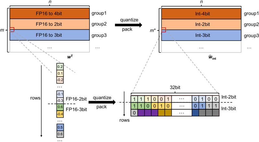
Figure 6: The memory layout shown in the figure is modified based on AutoGPTQ. The transposed original weights $\boldsymbol{w}^{\top}\in\mathbb{R}^{m\times n}$ are still divided into multiple groups along the row direction after quantization. The elements within each group are vertically packed into integers and then reassembled into $\hat{\boldsymbol{w}}_{\mathrm{int}}$. The figure employs corresponding colors to indicate how each original number is mapped to a specific position within the packed integers after quantization, which finally generates $\hat{\boldsymbol{w}}_{\mathrm{int}}\in\mathbb{R}^{m^{*}\times n}$, where $m^{*}$ is compressed from $m$ by packing several low-bit number. Similarly, $\hat{\boldsymbol{z}}_{\mathrm{int}}$ is also packed into integers to save memory.

Appendix C Searching Details of Group-Wise Salience-Determined Bit Allocation

We optimize the mixed-precision configuration based on the output information entropy (KL-divergence), searching for the optimal compensation bit-width ratio as shown in Eq. (4).

Initially, we rank each group by their average salience, a metric for quantization, and employ a double-pointer that moves simultaneously from both the beginning (lowest salience) and end (highest salience) of the sorted list. This ensures an equal number of groups at low and high bit-widths, effectively balancing the global average bit-width compensation. We then calculate the relative entropy under the corresponding precision ratio and search for the optimal ratio. Fig 7 displays the search error curves related to the $2^{nd}$, $10^{th}$, and $15^{th}$ Transformer layers in the OPT1.3B model, showcasing the search curves for certain self-attention layers (Query, Key, Value, FC2).

Due to the limited range of the search, extreme scenarios involve either a half ($N-1$)-bit and half ($N+1$)-bit without $N$-bit or all groups being $N$-bit (uniform precision). Fig 7 demonstrates that lower quantization errors can be achieved under mixed-precision compared to quantization at the uniform bit-width. We also find that multiple low-error precision combinations are possible within a group of weights, allowing SBA to flexibly select the optimal ratio through its versatile search.

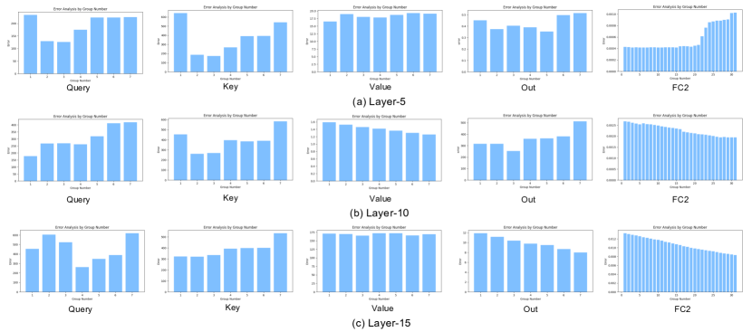
Figure 7: Error curves of SBA for select weights in the $5^{th}$, $10^{th}$, and $15^{th}$ layers of OPT-1.3B.

Appendix D Extension Ablation on SQC

In this section, we visualize the effectiveness of SQC in mitigating the degradation of information in locally salient weights. We observed the absolute error of weights in a randomly selected channel of the quantized OPT-1.3B model. As shown in Fig. 8, the overall absolute error of the weights post-quantization with a standard quantizer was 0.0055, while with SQC it was reduced to 0.0039. This further demonstrates that the search parameter $\gamma$, as applied in Eq. (5), effectively optimizes the quantizer parameters, thereby reducing quantization errors.

More importantly, SQC effectively perceives the information of locally salient weights, as indicated by the red regions in Fig. 8. Compared to the vanilla quantizer, SQC significantly reduces the error of salient weights. Specifically, the prominent weights at indices 375 in Fig. 8(a) show higher quantization errors, while in Fig. 8(b), this error is effectively reduced. This confirms SQC’s ability to perceive locally salient weights, effectively preventing the degradation of critical information.

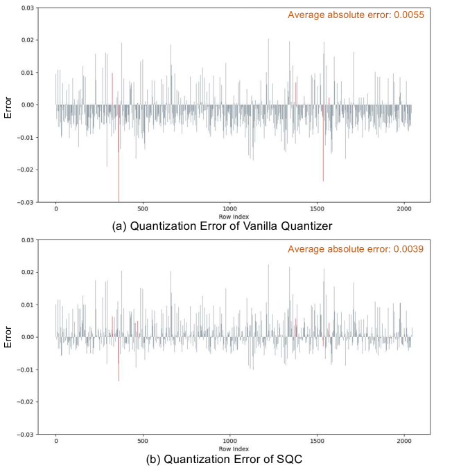
Figure 8: Absolute channel error of the weight of the OPT-1.3B model. The red line represents the quantization error for the locally salient weights, and the gray represents other weights. (a) Vanilla quantizer error on the $794^{th}$ channel of OPT-1.3B. (b) SQC error on the $794^{th}$ channel of OPT-1.3B

Appendix E Extension Ablation on Quantization Group-Size

To investigate the impact of different group sizes on the quantization effectiveness of SliM-LLM, we evaluated performance with 256 and 512 columns at a 3-bit level, observing that larger group sizes enhance GPU efficiency during inference. The findings suggest that increased group granularity does not substantially elevate perplexity across four models, indicating that SliM-LLM is robust and conducive to more efficient deployment methods. In contrast, at 2-bit, we assessed group sizes of 64 and 32 columns. With finer group granularity, the models displayed reduced perplexity. This is attributed to smaller groups providing more detailed data representation and utilizing additional quantization parameters, although they also raise computational and storage demands. A group size of 128 strikes a better balance between efficiency and quantization performance.

Table 5: Ablation results on OPT-6.7B, LLaMA-7B, LLaMA-2-7B, LLaMA-3-8B with SliM-LLM under different group size (#g denotes the group size).

Precision / PPL$\downarrow$	#g	OPT-6.7B	LLaMA-7B	LLaMA-2-7B	LLaMA-3-8B
3-bit	512	11.65	6.96	6.69	8.87
	256	11.33	6.92	6.94	8.14
	128	11.27	6.40	6.24	7.62
2-bit	128	14.41	14.58	16.01	39.66
	64	13.95	13.41	15.02	29.84
	32	12.47	11.91	11.95	16.93

Appendix F Extension on Salience Channel Clustering

F.1 Discussion of Theorem 1

Theorem 1.

Given the input calibration activation $\boldsymbol{x}\in\mathbb{R}^{t\times m}$ with an outlier value $x_{p,q}^{*}\gg x_{i,j},\forall i\in[0,t],i\neq p,\forall j\in[0,m],j\neq q$ at the position of token-$p$ and channel-$q$. The diagonal elements of $\boldsymbol{x}\boldsymbol{x}^{\top}$ also shows outlier value at $[\boldsymbol{x}\boldsymbol{x}^{\top}]_{p,p}$, as ${x_{p,q}^{*}}^{2}$ produced by $[\boldsymbol{x}\boldsymbol{x}^{\top}]_{i,i}=\sum_{k=1}^{n}x_{i,k}^{2}$ only appearing at position $(p,p)$, which further leads to the parameter salience larger at the $p^{th}$ channel of weight, where $\delta_{:,p}>\delta_{:,k},\delta_{:,k}=\frac{w_{:,k}^{2}}{[\boldsymbol{H}^{-1}]_{k,k}^{2}},\forall k\in[0,t],k\neq p$.

Proof.

Given $\boldsymbol{x}\in\mathbb{R}^{t\times m}$ with outlier value $x_{p,q}^{*}$ at token-$p$ and channel-$q$, $p\in[0,t]$ and $q\in[0,m]$, and other elements with small magnitude $x_{i,j}$, where $x_{p,q}^{*}\gg x_{i,j}$ and $i,j\neq p,q$. We can get the Hessian matrix with Levenberg-Marquardt [29] approximation in Eq. (3):

$$\begin{pmatrix}x_{11}&x_{12}&x_{13}&\cdots&x_{1m}\\ x_{21}&x_{22}&x_{23}&\cdots&x_{2m}\\ \vdots&\vdots&\vdots&\ddots&\vdots\\ \vdots&\vdots&\vdots&\boldsymbol{x_{p,q}^{*}}&\vdots\\ \vdots&\vdots&\vdots&\ddots&\vdots\\ x_{t1}&x_{t2}&x_{t3}&\cdots&x_{tm}\\ \end{pmatrix}\cdot\begin{pmatrix}x_{11}&x_{12}&\cdots&x_{1t}\\ x_{21}&x_{22}&\cdots&x_{2t}\\ \vdots&\vdots&\ddots&\vdots\\ \vdots&\vdots&\boldsymbol{x_{p,q}^{*}}&\vdots\\ \vdots&\vdots&\ddots&\vdots\\ x_{m1}&x_{m2}&\cdots&x_{mt}\\ \end{pmatrix}=\begin{pmatrix}x_{11}^{2}..&\cdots&\cdots&\cdots\\ \vdots&\ddots&\cdots&\vdots\\ \vdots&\vdots&\boldsymbol{x_{p,q}^{*}}^{2}..&\vdots\\ \cdots&\cdots&\cdots&\ddots\\ \end{pmatrix}$$ (7)

where ${x_{p,q}^{*}}^{2}$ only appears at position $\boldsymbol{H}_{p,p}$. And following SparseGPT [15], the inverse matrix of $\boldsymbol{H}$ can be formulated as:

$$\delta_{i,j}=\frac{w_{i,j}^{2}}{[\operatorname{diag}((\boldsymbol{x}\boldsymbol{x}^{\top}+\lambda\boldsymbol{I})^{-1})]^{2}}$$ (8)

where $(\boldsymbol{x}\boldsymbol{x}^{\top}+\lambda\boldsymbol{I})^{-1}$ is the new representation of Hessian matrix $\boldsymbol{H}$ for the layer-wise reconstruction problem, and $\lambda$ is the dampening factor for the Hessian to prevent the collapse of the inverse computation. Additionally, in accordance with the configuration in LLMs [15, 16, 39], the value of $\lambda$ set is extremely small ($\lambda\leq e^{-1}$), while the values located at the diagonal of Hessian are large. Therefore, only considering the influence of diagonal elements [39], we can further approximate salience as:

$$\delta_{i,j}=\frac{w_{i,j}^{2}}{[\operatorname{diag}((\boldsymbol{x}\boldsymbol{x}^{\top}+\lambda\boldsymbol{I})^{-1})]^{2}}\approx\frac{w_{i,j}^{2}}{[(\operatorname{diag}(\boldsymbol{x}\boldsymbol{x}^{\top}))^{-1}]^{2}}=(w_{i,j}\cdot||\boldsymbol{x}_{j}||_{2}^{2})^{2}$$ (9)

Here the diagonal of $\boldsymbol{x}\boldsymbol{x}^{\top}$ is $\operatorname{diag}(||\boldsymbol{x}_{j}||_{2}^{2})$, and $||\boldsymbol{x}_{j}||_{2}$ evaluates the $\ell_{2}$ norm of $j^{th}$ channel across different tokens. Consequently, it can be summarized that when there is an outlier value at the position of the token-$p$ and channel-$q$, $||\boldsymbol{x}_{p}||_{2}$ is primarily influenced by $x_{p,q}^{*}$. Additionally, since the activation values are relatively large and the differences in weight values are comparatively small, the $p^{th}$ channel of weights will also exhibit salience. ∎

F.2 Distribution of salience, activation and weight magnitude

Fig. 9 illustrates the distribution of salience among certain weights in LLMs. This section provides additional examples to demonstrate how the distribution of weights and input activation characteristics influence the salience of parameters in LLMs. The figure captures seven linear projections in the multi-head self-attention (MHA) and feed-forward block (FFB) layers of the $2^{nd}$ and $10^{th}$ Transformer modules in the LLaMA-7B model.

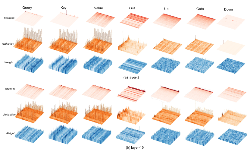
Figure 9: Salience, activation and weight distribution in the $2^{nd}$ and $10^{th}$ layers of LLaMA-7B

In line with previous findings [32, 44], activations demonstrate particularly marked outlier phenomena on anomalous tokens and channels, with extremes differing by more than two orders of magnitude. Notably, distinct anomalous channels are present in the MHA’s Query, Key, and Value layers, where outliers vary significantly across different tokens. This pattern is consistent in the FFB layers. We observe that disparities in weight magnitudes are less pronounced than those in activation, thus exerting a reduced impact on outlier channels. Moreover, weights exhibit structured distributions along rows or columns [12, 20], affecting the overall distribution of salience from a row-wise perspective (Fig. 9). However, the most prominent salience is predominantly driven by activation across channels (column-wise).

F.3 Hessian Diagonal Clustering

Sec. 3.2.1 demonstrates that outlier tokens in input activations result in significant values at the corresponding positions along the diagonal of the weight Hessian matrix. Additionally, due to the token sink phenomenon [45, 32], areas around significantly activated key tokens exhibit increased salience, creating clusters of salient regions along the Hessian matrix diagonal. To further elucidate this phenomenon, Fig. 10 shows the values along the diagonal of the Hessian matrix for selected weights in the $2^{nd}$ and $10^{th}$ layers of the LLaMA-7B model. Within this diagonal, certain positions display pronounced values (indicated in red), whereas others are relatively moderate. In the attention aggregation layer of the $10^{th}$ layer, the token sink phenomenon results in a pronounced convergence of significant values along the Hessian matrix diagonal, with deep red areas indicating regional clustering. These findings reinforce the influence of input activations on the diagonal of the Hessian matrix, subsequently leading to a clustering phenomenon in the salience distribution of weights across channels.

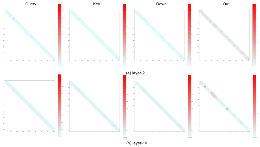
Figure 10: Hessian diagonal magnitude in attention layers of $2^{nd}$ and $10^{th}$ layers of LLaMA-7B

Appendix G More Comparisons

In this section, we provide supplementary experiments for SliM-LLM. Tab. 6 displays the comparative results of SliM-LLM and SliM-LLM* with other methods on the OPT series models. Tab. 7 shows the performance of SliM-LLM when quantizing the LLaMA family models on the C4 dataset, while Tab. 8 also compares the results of SliM-LLM* on the C4 dataset.

Table 6: Quantization results of OPT Models on WikiText2 (group size is 128).

#W PPL$\downarrow$	Method	1.3B	2.7B	6.7B	13B	30B	66B
16-bit	-	14.63	12.47	10.86	10.12	9.56	9.34
3-bit	RTN	1.2e2	3.0e2	23.54	46.03	18.80	1.4e6
	GPTQ	16.47	13.69	11.65	10.35	9.73	10.96
	AWQ	16.32	13.58	11.41	10.68	9.85	9.60
	QuIP	16.21	13.79	11.51	10.50	9.75	9.59
	SliM-LLM	15.91	13.26	11.27	10.26	9.70	9.48
2-8	OmniQuant	15.72	13.18	11.27	10.47	9.79	9.53
	AffineQuant	15.61	12.98	11.18	10.51	9.81	-
	SliM-LLM+	15.58	12.84	11.18	10.44	9.67	9.51
2-bit	RTN	1.3e4	5.7e4	7.8e3	7.6e4	1.3e4	3.6e5
	GPTQ	1.1e2	61.59	20.18	21.36	12.71	82.10
	AWQ	47.97	28.50	16.20	14.32	12.31	14.54
	QuIP	41.64	28.98	18.57	16.02	11.48	10.76
	PB-LLM	45.92	39.71	20.37	19.11	17.01	16.36
	SliM-LLM	30.71	24.08	14.41	13.68	11.34	10.94
2-8	OmniQuant	23.95	18.13	14.43	12.94	11.39	30.84
	SliM-LLM+	24.57	17.98	14.22	12.16	11.27	14.98

Table 7: Quantization results of LLaMA Family with statistic quantizer on C4 (group size is 128).

#W PPL$\downarrow$	Method	1-7B	1-13B	1-30B	1-65B	2-7B	2-13B	2-70B	3-8B	3-70B
16-bit	-	7.08	6.61	5.98	5.62	6.97	6.46	5.52	9.22	6.85
3-bit	APTQ	6.24	-	-	-	-	-	-	-	-
	RTN	8.62	7.49	6.58	6.10	8.40	7.18	6.02	1.1e2	22.39
	AWQ	7.92	7.07	6.37	5.94	7.84	6.94	-	11.62	8.03
	GPTQ	7.85	7.10	6.47	6.00	7.89	7.00	5.85	13.67	10.52
	SliM-LLM	6.14	6.05	6.33	5.94	7.74	5.26	5.09	13.10	8.64
2-bit	RTN	1.0e3	4.5e2	99.45	17.15	4.9e3	1.4e2	42.13	2.5e4	4.6e5
	AWQ	1.9e5	2.3e5	2.4e5	7.5e4	1.7e5	9.4e4	-	2.1e6	1.4e6
	GPTQ	34.63	15.29	11.93	11.99	33.70	20.97	NAN	4.1e4	21.82
	QuIP	33.74	21.94	10.95	13.99	31.94	16.16	8.17	1.3e2	22.24
	PB-LLM	49.73	26.93	17.93	11.85	29.84	19.82	8.95	79.21	33.91
	SliM-LLM	32.91	13.85	11.27	10.95	16.00	9.41	7.01	1.1e2	15.92

Table 8: Quantization results of LLaMA-1 and LLaMA-2 models with learnable quantizer on C4.

#W PPL$\downarrow$	Method	1-7B	1-13B	1-30B	1-65B	2-7B	2-13B	2-70B
16-bit	-	7.08	6.61	5.98	5.62	6.97	6.46	5.52
3-bit	OmniQuant	7.75	7.05	6.37	5.93	7.75	6.98	5.85
	AffineQuant	7.75	7.04	6.40	-	7.83	6.99	-
	SliM-LLM+	7.75	6.91	6.36	5.96	7.71	6.90	5.85
2-bit	OmniQuant	12.97	10.36	9.36	8.00	15.02	11.05	8.52
	AffineQuant	14.92	12.64	9.66	-	16.02	10.98	-
	SliM-LLM+	14.99	10.22	9.33	7.52	18.18	10.24	8.40

Appendix H Real Dialog Examples

In this section, we show some dialogue examples of LLaMA-2-13B and Vicuna-13B with SliM-LLM-2bit and GPTQ-2bit in Fig. 11.

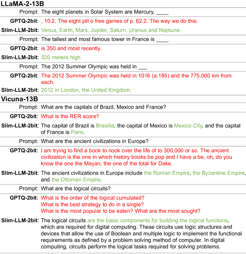
Figure 11: Some examples of conversations. LLaMA-2-13B and Vicuna-13B are chosen to show the case of language supplementary and Q&A ability. And GPTQ-2bit is selected as the comparison. We color the text to show the reasonable or inappropriate responses.

References

- [1] Josh Achiam, Steven Adler, Sandhini Agarwal, Lama Ahmad, Ilge Akkaya, Florencia Leoni Aleman, Diogo Almeida, Janko Altenschmidt, Sam Altman, Shyamal Anadkat, et al. GPT-4 technical report. arXiv preprint arXiv:2303.08774, 2023.
- [2] Yonatan Bisk, Rowan Zellers, Jianfeng Gao, Yejin Choi, et al. Piqa: Reasoning about physical commonsense in natural language. In Proceedings of the AAAI conference on artificial intelligence, volume 34, pages 7432–7439, 2020.
- [3] Tom Brown, Benjamin Mann, Nick Ryder, Melanie Subbiah, Jared D Kaplan, Prafulla Dhariwal, Arvind Neelakantan, Pranav Shyam, Girish Sastry, Amanda Askell, et al. Language models are few-shot learners. Advances in Neural Information Processing Systems, 33:1877–1901, 2020.
- [4] Sébastien Bubeck, Varun Chandrasekaran, Ronen Eldan, Johannes Gehrke, Eric Horvitz, Ece Kamar, Peter Lee, Yin Tat Lee, Yuanzhi Li, Scott Lundberg, et al. Sparks of artificial general intelligence: Early experiments with GPT-4. arXiv preprint arXiv:2303.12712, 2023.
- [5] Yupeng Chang, Xu Wang, Jindong Wang, Yuan Wu, Linyi Yang, Kaijie Zhu, Hao Chen, Xiaoyuan Yi, Cunxiang Wang, Yidong Wang, et al. A survey on evaluation of large language models. ACM Transactions on Intelligent Systems and Technology, 15(3):1–45, 2024.
- [6] Jerry Chee, Yaohui Cai, Volodymyr Kuleshov, and Christopher M De Sa. Quip: 2-bit quantization of large language models with guarantees. Advances in Neural Information Processing Systems, 36, 2024.
- [7] Hong Chen, Chengtao Lv, Liang Ding, Haotong Qin, Xiabin Zhou, Yifu Ding, Xuebo Liu, Min Zhang, Jinyang Guo, Xianglong Liu, et al. DB-LLM: Accurate dual-binarization for efficient llms. arXiv preprint arXiv:2402.11960, 2024.
- [8] Wei-Lin Chiang, Zhuohan Li, Zi Lin, Ying Sheng, Zhanghao Wu, Hao Zhang, Lianmin Zheng, Siyuan Zhuang, Yonghao Zhuang, Joseph E Gonzalez, et al. Vicuna: An open-source chatbot impressing GPT-4 with 90%* chatgpt quality. See https://vicuna. lmsys. org (accessed 14 April 2023), 2023.
- [9] Christopher Clark, Kenton Lee, Ming-Wei Chang, Tom Kwiatkowski, Michael Collins, and Kristina Toutanova. BoolQ: Exploring the surprising difficulty of natural yes/no questions. arXiv preprint arXiv:1905.10044, 2019.
- [10] Peter Clark, Isaac Cowhey, Oren Etzioni, Tushar Khot, Ashish Sabharwal, Carissa Schoenick, and Oyvind Tafjord. Think you have solved question answering? try arc, the ai2 reasoning challenge. arXiv preprint arXiv:1803.05457, 2018.
- [11] Tim Dettmers, Mike Lewis, Younes Belkada, and Luke Zettlemoyer. LLM.int8 (): 8-bit matrix multiplication for transformers at scale. arXiv preprint arXiv:2208.07339, 2022.
- [12] Tim Dettmers, Ruslan Svirschevski, Vage Egiazarian, Denis Kuznedelev, Elias Frantar, Saleh Ashkboos, Alexander Borzunov, Torsten Hoefler, and Dan Alistarh. SpQR: A sparse-quantized representation for near-lossless LLM weight compression. arXiv preprint arXiv:2306.03078, 2023.
- [13] Vage Egiazarian, Andrei Panferov, Denis Kuznedelev, Elias Frantar, Artem Babenko, and Dan Alistarh. Extreme compression of large language models via additive quantization. arXiv preprint arXiv:2401.06118, 2024.
- [14] Elias Frantar and Dan Alistarh. Optimal brain compression: A framework for accurate post-training quantization and pruning. Advances in Neural Information Processing Systems, 35:4475–4488, 2022.
- [15] Elias Frantar and Dan Alistarh. SparseGPT: Massive language models can be accurately pruned in one-shot. In International Conference on Machine Learning, pages 10323–10337. PMLR, 2023.
- [16] Elias Frantar, Saleh Ashkboos, Torsten Hoefler, and Dan Alistarh. GPTQ: Accurate post-training quantization for generative pre-trained transformers. arXiv preprint arXiv:2210.17323, 2022.
- [17] Prakhar Ganesh, Yao Chen, Xin Lou, Mohammad Ali Khan, Yin Yang, Hassan Sajjad, Preslav Nakov, Deming Chen, and Marianne Winslett. Compressing large-scale transformer-based models: A case study on bert. Transactions of the Association for Computational Linguistics, 9:1061–1080, 2021.
- [18] Ziyi Guan, Hantao Huang, Yupeng Su, Hong Huang, Ngai Wong, and Hao Yu. APTQ: Attention-aware post-training mixed-precision quantization for large language models. arXiv preprint arXiv:2402.14866, 2024.
- [19] Dan Hendrycks, Collin Burns, Steven Basart, Andy Zou, Mantas Mazeika, Dawn Song, and Jacob Steinhardt. Measuring massive multitask language understanding. arXiv preprint arXiv:2009.03300, 2020.
- [20] Wei Huang, Yangdong Liu, Haotong Qin, Ying Li, Shiming Zhang, Xianglong Liu, Michele Magno, and Xiaojuan Qi. BiLLM: Pushing the limit of post-training quantization for llms. arXiv preprint arXiv:2402.04291, 2024.
- [21] Wei Huang, Xudong Ma, Haotong Qin, Xingyu Zheng, Chengtao Lv, Hong Chen, Jie Luo, Xiaojuan Qi, Xianglong Liu, and Michele Magno. How Good Are Low-bit Quantized LLaMA3 Models? An Empirical Study. arXiv preprint arXiv:2404.14047, 2024.
- [22] Aravindh Krishnamoorthy and Deepak Menon. Matrix inversion using cholesky decomposition. In 2013 signal processing: Algorithms, architectures, arrangements, and applications (SPA), pages 70–72. IEEE, 2013.
- [23] Changhun Lee, Jungyu Jin, Taesu Kim, Hyungjun Kim, and Eunhyeok Park. OWQ: Lessons learned from activation outliers for weight quantization in large language models. arXiv preprint arXiv:2306.02272, 2023.
- [24] Shiyao Li, Xuefei Ning, Ke Hong, Tengxuan Liu, Luning Wang, Xiuhong Li, Kai Zhong, Guohao Dai, Huazhong Yang, and Yu Wang. LLM-MQ: Mixed-precision quantization for efficient LLM deployment. In Advances in Neural Information Processing Systems (NeurIPS) ENLSP Workshop, 2024.
- [25] Yanwei Li, Yuechen Zhang, Chengyao Wang, Zhisheng Zhong, Yixin Chen, Ruihang Chu, Shaoteng Liu, and Jiaya Jia. Mini-gemini: Mining the potential of multi-modality vision language models. arXiv preprint arXiv:2403.18814, 2024.
- [26] Ji Lin, Jiaming Tang, Haotian Tang, Shang Yang, Xingyu Dang, and Song Han. AWQ: Activation-aware weight quantization for LLM compression and acceleration. arXiv preprint arXiv:2306.00978, 2023.
- [27] Zechun Liu, Barlas Oguz, Changsheng Zhao, Ernie Chang, Pierre Stock, Yashar Mehdad, Yangyang Shi, Raghuraman Krishnamoorthi, and Vikas Chandra. LLM-QAT: Data-Free Quantization Aware Training for Large Language Models. arXiv preprint arXiv:2305.17888, 2023.
- [28] Yuexiao Ma, Huixia Li, Xiawu Zheng, Feng Ling, Xuefeng Xiao, Rui Wang, Shilei Wen, Fei Chao, and Rongrong Ji. Affinequant: Affine transformation quantization for large language models. arXiv preprint arXiv:2403.12544, 2024.
- [29] Donald W Marquardt. An algorithm for least-squares estimation of nonlinear parameters. Journal of the society for Industrial and Applied Mathematics, 11(2):431–441, 1963.
- [30] Stephen Merity, Caiming Xiong, James Bradbury, and Richard Socher. Pointer sentinel mixture models. arXiv preprint arXiv:1609.07843, 2016.
- [31] Markus Nagel, Rana Ali Amjad, Mart Van Baalen, Christos Louizos, and Tijmen Blankevoort. Up or down? adaptive rounding for post-training quantization. In International Conference on Machine Learning, pages 7197–7206. PMLR, 2020.
- [32] Aniruddha Nrusimha, Mayank Mishra, Naigang Wang, Dan Alistarh, Rameswar Panda, and Yoon Kim. Mitigating the impact of outlier channels for language model quantization with activation regularization. arXiv preprint arXiv:2404.03605, 2024.
- [33] Haotong Qin, Xudong Ma, Xingyu Zheng, Xiaoyang Li, Yang Zhang, Shouda Liu, Jie Luo, Xianglong Liu, and Michele Magno. Accurate LoRA-Finetuning Quantization of LLMs via Information Retention. arXiv preprint arXiv:2402.05445, 2024.
- [34] Haotong Qin, Mingyuan Zhang, Yifu Ding, Aoyu Li, Zhongang Cai, Ziwei Liu, Fisher Yu, and Xianglong Liu. Bibench: Benchmarking and analyzing network binarization. arXiv preprint arXiv:2301.11233, 2023.
- [35] Haotong Qin, Xiangguo Zhang, Ruihao Gong, Yifu Ding, Yi Xu, and Xianglong Liu. Distribution-sensitive information retention for accurate binary neural network. International Journal of Computer Vision, 131(1):26–47, 2023.
- [36] Colin Raffel, Noam Shazeer, Adam Roberts, Katherine Lee, Sharan Narang, Michael Matena, Yanqi Zhou, Wei Li, and Peter J Liu. Exploring the limits of transfer learning with a unified text-to-text transformer. The Journal of Machine Learning Research, 21(1):5485–5551, 2020.
- [37] Yuzhang Shang, Zhihang Yuan, Qiang Wu, and Zhen Dong. PB-LLM: Partially binarized large language models. arXiv preprint arXiv:2310.00034, 2023.
- [38] Wenqi Shao, Mengzhao Chen, Zhaoyang Zhang, Peng Xu, Lirui Zhao, Zhiqian Li, Kaipeng Zhang, Peng Gao, Yu Qiao, and Ping Luo. Omniquant: Omnidirectionally calibrated quantization for large language models. arXiv preprint arXiv:2308.13137, 2023.
- [39] Mingjie Sun, Zhuang Liu, Anna Bair, and J Zico Kolter. A simple and effective pruning approach for large language models. arXiv preprint arXiv:2306.11695, 2023.
- [40] Gemini Team, Rohan Anil, Sebastian Borgeaud, Yonghui Wu, Jean-Baptiste Alayrac, Jiahui Yu, Radu Soricut, Johan Schalkwyk, Andrew M Dai, Anja Hauth, et al. Gemini: a family of highly capable multimodal models. arXiv preprint arXiv:2312.11805, 2023.
- [41] Hugo Touvron, Thibaut Lavril, Gautier Izacard, Xavier Martinet, Marie-Anne Lachaux, Timothée Lacroix, Baptiste Rozière, Naman Goyal, Eric Hambro, Faisal Azhar, et al. Llama: Open and efficient foundation language models. arXiv preprint arXiv:2302.13971, 2023.
- [42] Hugo Touvron, Louis Martin, Kevin Stone, Peter Albert, Amjad Almahairi, Yasmine Babaei, Nikolay Bashlykov, Soumya Batra, Prajjwal Bhargava, Shruti Bhosale, et al. Llama 2: Open foundation and fine-tuned chat models. arXiv preprint arXiv:2307.09288, 2023.
- [43] Albert Tseng, Jerry Chee, Qingyao Sun, Volodymyr Kuleshov, and Christopher De Sa. Quip#: Even better LLM quantization with hadamard incoherence and lattice codebooks. arXiv preprint arXiv:2402.04396, 2024.
- [44] Guangxuan Xiao, Ji Lin, Mickael Seznec, Hao Wu, Julien Demouth, and Song Han. Smoothquant: Accurate and efficient post-training quantization for large language models. In International Conference on Machine Learning, pages 38087–38099. PMLR, 2023.
- [45] Guangxuan Xiao, Yuandong Tian, Beidi Chen, Song Han, and Mike Lewis. Efficient streaming language models with attention sinks. arXiv preprint arXiv:2309.17453, 2023.
- [46] Yuhui Xu, Lingxi Xie, Xiaotao Gu, Xin Chen, Heng Chang, Hengheng Zhang, Zhensu Chen, Xiaopeng Zhang, and Qi Tian. Qa-lora: Quantization-aware low-rank adaptation of large language models. arXiv preprint arXiv:2309.14717, 2023.
- [47] Z Yao, RY Aminabadi, M Zhang, X Wu, C Li, and Y Zeroquant He. Efficient and affordable post-training quantization for large-scale transformers. URL https://arxiv. org/abs/2206.01861, 2022.
- [48] Rowan Zellers, Ari Holtzman, Yonatan Bisk, Ali Farhadi, and Yejin Choi. Hellaswag: Can a machine really finish your sentence? arXiv preprint arXiv:1905.07830, 2019.
- [49] Susan Zhang, Stephen Roller, Naman Goyal, Mikel Artetxe, Moya Chen, Shuohui Chen, Christopher Dewan, Mona Diab, Xian Li, Xi Victoria Lin, et al. Opt: Open pre-trained transformer language models. arXiv preprint arXiv:2205.01068, 2022.
- [50] Yiyuan Zhang, Kaixiong Gong, Kaipeng Zhang, Hongsheng Li, Yu Qiao, Wanli Ouyang, and Xiangyu Yue. Meta-transformer: A unified framework for multimodal learning. arXiv preprint arXiv:2307.10802, 2023.
- [51] Wayne Xin Zhao, Kun Zhou, Junyi Li, Tianyi Tang, Xiaolei Wang, Yupeng Hou, Yingqian Min, Beichen Zhang, Junjie Zhang, Zican Dong, et al. A survey of large language models. arXiv preprint arXiv:2303.18223, 2023.
- [52] Xunyu Zhu, Jian Li, Yong Liu, Can Ma, and Weiping Wang. A survey on model compression for large language models. arXiv preprint arXiv:2308.07633, 2023.