Static and dynamic properties of atomic nuclei with high-resolution potentials
Abstract
We compute ground-state and dynamical properties of 4He and 16O nuclei using as input high-resolution, phenomenological nucleon-nucleon and three-nucleon forces that are local in coordinate space. The nuclear Schrödinger equation for both nuclei is accurately solved employing the auxiliary-field diffusion Monte Carlo approach. For the 4He nucleus, detailed benchmarks are carried out with the hyperspherical harmonics method. In addition to presenting results for the binding energies and radii, we also analyze the momentum distributions of these nuclei and their Euclidean response function corresponding to the isoscalar density transition. The latter quantity is particularly relevant for lepton-nucleus scattering experiments, as it paves the way to quantum Monte Carlo calculations of electroweak response functions of 16O.
I Introduction
Tremendous progress has been made in the last two decades in computing properties of atomic nuclei and infinite nuclear matter starting from non-relativistic potentials modeling the individual interactions among protons and neutrons. After the seminal works by Weinberg Weinberg (1990, 1991), two- and three-body potentials are nowadays systematically derived starting from an effective Lagrangian, constrained by the broken chiral symmetry pattern of QCD, Epelbaum et al. (2009); Machleidt and Entem (2011); Reinert et al. (2018); Entem et al. (2017). Chiral effective field theory (EFT) potentials serve as input to advanced quantum many-body approaches, suitable to solving the nuclear Schrödinger equation Carbone et al. (2013); Barrett et al. (2013); Hagen et al. (2014); Carlson et al. (2015); Hergert et al. (2016); Lynn et al. (2019). Among them, methods relying on single-particle basis expansion can treat nuclei up to 208Pb Hu et al. (2022); Malbrunot-Ettenauer et al. (2022), including radii, electromagnetic transitions Lechner et al. (2023), single -decay and double- decay rates Gysbers et al. (2019).
The convergence of the single-particle basis method is greatly aided by the softness of the potential. In addition to the chiral symmetry breaking scale, GeV, the range of applicability of EFT interactions, or their resolution scale, is also determined by a regulator function that smoothly truncates one- and two-pion exchange interactions at short distances. Commonly used chiral forces, such as NNLO Ekström et al. (2013), NNLO Ekström et al. (2015), and NNLOGO Jiang et al. (2020), are characterized by relatively small regulator values. Low-resolution observables like binding energies, radii, and electroweak transitions can be accurately computed using these relatively low-resolution Hamiltonians. In fact, it has been shown that even lower-resolution interactions can reproduce these quantities within a few percent from their experimental values Lu et al. (2019); Gattobigio et al. (2019); Kievsky et al. (2021); Schiavilla et al. (2021); Lovato et al. (2022a); Gnech et al. (2023).
The limitations of EFT Hamiltonians become apparent when dealing with observables sensitive to short-range dynamics. An illustrative instance is the equation of state of neutron-star matter at densities beyond nuclear saturation Lovato et al. (2022b). The Authors of this reference found that certain local, -full EFT Hamiltonians, that accurately reproduce the light nuclei spectrum Piarulli et al. (2018); Baroni et al. (2018), yield self-bound neutron matter Lovato et al. (2022b). This un-physical behavior, characterized by closely packed neutron clusters, arises from the attractive nature of the three-body force contact term. The latter does not vanish in neutron matter because of regulator artifacts Lovato et al. (2012). Similarly, a dramatic overbinding of nuclear matter and no saturation at reasonable densities is obtained using the set of EFT potentials Hüther et al. (2020) that reproduce accurately experimental energies and radii of nuclei up to 78Ni Sammarruca and Millerson (2020).
Highly realistic, phenomenological nucleon-nucleon (NN) forces, such as the Argonne (AV18) Wiringa et al. (1995) are constructed to reproduce nucleon-nucleon scattering data with up to energies corresponding to pion-production threshold. However, their predictions remain accurate even at larger energies Benhar (2021), so as they can be identified as “high-resolution” potentials. The remarkable accuracy of the Argonne interactions has been recently highlighted by the analysis of semi-exclusive electron-scattering data Schmidt et al. (2020), which are extremely sensitive to short-range correlated pairs in nuclei. In addition, their connection with the equation of state of neutron-star matter has been pointed out in Ref. Benhar (2021). Nonetheless, these phenomenological potentials have several shortcomings. The Argonne plus Illinois 7 Pieper (2008) (IL7) Hamiltonian can reproduce the experimental energies of nuclei with up to with high precision, but it fails to provide sufficient repulsion in pure neutron matter Maris et al. (2013). On the other hand, the Argonne plus Urbana IX (UIX) model, while providing a good description of nuclear-matter properties, does not satisfactorily reproduce the spectrum of light nuclei Pieper et al. (2001). As these Hamiltonians are phenomenological in nature, no clear prescriptions are available to properly assess their uncertainties and to systematically improve them.
In this work, we carry out high-resolution calculation of 4He, and 16O static and dynamic properties, including binding energies, radii, momentum distribution and isoscalar density response functions. We focus on phenomenological Hamiltonians of the Argonne family, specifically on the Argonne (AV8P) and Argonne (AV6P) NN forces Wiringa and Pieper (2002) supplemented by the consistent Urbana IX (UIX) 3N interaction Pudliner et al. (1995). To gauge the accuracy in solving the quantum many-body problem, for the 4He nucleus, we benchmark the auxiliary-field diffusion Monte Carlo (AFDMC) with the highly-accurate hyper-spherical harmonics (HH) method Kievsky et al. (2008); Marcucci et al. (2020). This comparison is particularly relevant for quantifying the approximations made in the imaginary-time propagation upon which the AFDMC is based. We note that useful benchmarks among different many-body methods have been carried out for both nuclei Kamada et al. (2001); Hagen et al. (2007); Tichai et al. (2020), and infinite neutron matter Ref. Baldo et al. (2012); Piarulli et al. (2020); Lovato et al. (2022b).
This article is organized as follows. In Section II we introduce the nuclear Hamiltonian and the quantum many-body methods of choice. Section III is devoted to the results, including a detailed comparison between the HH and AFDMC methods. Finally, in Section IV we draw our conclusions and discuss future perspectives of this work.
II Methods
II.1 Phenomenological Nuclear Hamiltonians
To a remarkably large extent, the dynamics of atomic nuclei can be accurately modeled employing a non-relativistic Hamiltonian
| (1) |
where and denote the momentum of the -th nucleon and its mass, and the potentials and describe nucleon-nucleon (NN) and three-nucleon (3N) interactions, respectively. Highly-realistic, phenomenological NN potentials, such as the AV18 Wiringa et al. (1995), are fitted to reproduce the observed properties of the two-nucleon system, including the deuteron binding energy, magnetic moment and electric quadrupole moment, as well as the data obtained from the measured NN scattering cross sections—and reduce to Yukawa’s one-pion-exchange potential at large distance. They are usually defined in coordinate space as
| (2) |
with . The bulk of the interaction is encoded in the first eight operators
| (3) |
In the above equation we introduced and with and being the Pauli matrices acting in the spin and isospin space. The tensor operator is given by
| (4) |
while the spin-orbit contribution is expressed in terms of the relative angular momentum and the total spin of the pair. AV18 contains six additional charge-independent operators corresponding to that are quadratic in , while the are charge-independence breaking terms.
It is useful to define simpler versions of the AV18 potentials with fewer operators: the (AV8P) with the eight operators of Eq. (3) and the (AV6P) without the terms Wiringa and Pieper (2002). AV8P is a reprojection (rather than a simple truncation) of the strong-interaction potential that reproduces the charge-independent average of 1S0, 3S1-3D1, 1P1, 3P0, 3P1, and (almost) 3P2 phase shifts by construction, while overbinding the deuteron by keV due to the omission of electromagnetic terms. AV6P is (mostly) a truncation of AV8P that reproduces 1S0 and 1P1 partial waves, makes a slight adjustment to (almost) match the deuteron and 3S1-3D1 partial waves, but will no longer split the 3PJ partial waves properly.
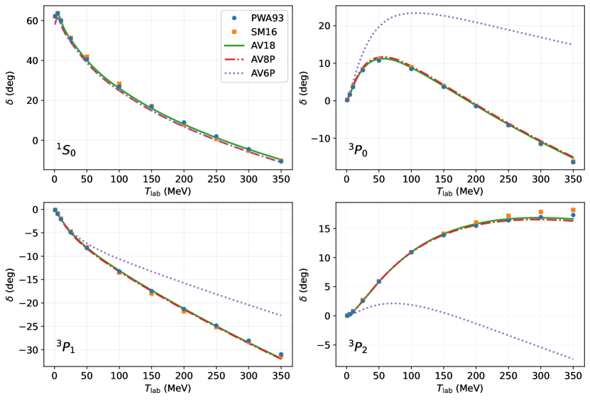
Fig.1 illustrates the energy dependence of the proton-neutron scattering phase shifts in the 1S0, 3P0, 3P1, and 3P2 partial waves, comparing the AV6P, AV8P, and AV18 potentials with the experimental analysis of Refs.Stoks et al. (1993); Workman et al. (2016). The AV18 interaction provides an accurate description of the scattering data up to MeV in all channels. All potentials reproduce the channel very well, as neither spin-orbit nor tensor components are active there. On the other hand, in the , , and channels, the AV6P potential deviates from the AV18 results, particularly in the wave. These shortcomings, which can be ascribed to the missing spin-orbit components, are not present in the AV8P potential, which reproduces all -wave phase shifts. Discrepancies between AV8P and AV18 appear in higher partial waves.
In this work, we assume the electromagnetic component of the NN potential to only include the Coulomb force between finite-size protons.
The earliest example of a three-body force in nuclear physics dates back to the Fujita-Miyazawa interaction, whose main contributions arises from the virtual excitation of a resonance in processes involving three interacting nucleons Fujita and Miyazawa (1957). This term is included in the UIX potential as
| (5) |
The “commutator” and “commutator” contributions are given by
| (6) |
where denotes a sum over the three cyclic exchanges of nucleons . The operator is defined as
| (7) |
where the normal Yukawa and tensor functions are
| (8) |
and the short-range regulator is taken to be with fm-2. In the UIX model, it is assumed that as in the original Fujita-Miyazawa formulation. We note however that other ratios slightly larger than have been considered in the Tucson-Melbourne Coon et al. (1979) and Brazil Coelho et al. (1983) models of the 3N force. Generally, a 3N potential only comprised of does not yield the correct isospin-symmetric nucleonic matter saturation density Lagaris and Pandharipande (1981) and a repulsive 3N force should be included
| (9) |
The constants and entering the UIX model are determined by fitting the binding energy of 3H and the saturation density of isospin-symmetric nucleonic matter fm-3. More sophisticated phenomenological 3N interactions have been developed, such as the IL7 Pieper (2008), but we will not consider them here as they fail to provide sufficient repulsion in pure neutron matter Maris et al. (2013). Rather, we stick to the UIX model, although it underbinds light p-shell nuclei — and in particular it is not possible to fit both 8He and 8Be at the same time Carlson et al. (2015).
II.2 Auxiliary field diffusion Monte Carlo
The AFDMC method Schmidt and Fantoni (1999) leverages imaginary-time projection techniques to filter out the ground-state of the system starting from a suitable variational wave function
| (10) |
In the above equation is a normalization constant, which is chosen to be close to the true ground-state energy .
The variational wave function is expressed as a product of a long and a short-range parts . To fix the notation, let denote the set of single-particle coordinates , which describe the spatial positions and the spin-isospin degrees of freedom of the nucleons. The long-range behavior of the wave function is described by the Slater determinant
| (11) |
The symbol denotes the antisymmetrization operator and represent the quantum numbers of the single-particle orbitals. The latter are expressed as
| (12) |
where the spherical harmonics are coupled to the spinor to get the single-particle orbitals in the basis and describes the isospin single-particle state. The radial functions are parametrized in terms of cubic splines Contessi et al. (2017).
Since the Hamiltonians considered in this work contain tensor and spin-orbit interactions, we consider a variational wave function that includes two- and three-body correlations
| (13) |
To keep a polynomial cost in the number of nucleons, as in Ref. Gandolfi et al. (2014), we approximate the spin-isospin correlations to a linear form
| (14) |
where the operators are defined in Eq. (3). The functions are characterized by a number of variational parameters Gandolfi et al. (2020), which are determined by minimizing the two-body cluster contribution to the energy per particle of nuclear matter at saturation density.
The spin-isospin dependent three-body correlations are derived within perturbation theory as Carlson et al. (2015); Lonardoni et al. (2018); Gandolfi et al. (2020)
| (15) |
with being a variational parameter. Finally, the scalar three-body correlation is expressed as
| (16) |
Both the three-body correlations , the scalar two-body Jastrow are parametrized in terms of cubic splines Contessi et al. (2017). The variational parameters are the values of and at the grid points, plus the value of their first derivatives at . The optimal values of the variational parameters are found employing the linear optimization method Toulouse and Umrigar (2007); Contessi et al. (2017), which typically converges in about iterations. We note that variational states based on neural network quantum states have been recently proposed Adams et al. (2021); Gnech et al. (2022); Lovato et al. (2022a); Gnech et al. (2023). Their use in AFDMC calculations will be the subject of future works.
The imaginary-time propagator is broken down in small time steps , with . At each step, the generalized coordinates are sampled from the previous ones according to the short-time propagator
| (17) |
where is the importance-sampling function. Similar to Refs. Zhang et al. (1997); Zhang and Krakauer (2003), we mitigate the fermion-sign problem by first performing a constrained-path diffusion Monte Carlo propagation (DMC-CP), in which we take and impose . The energy computed during a DMC-CP is not a rigorous upper-bound to Wiringa et al. (2000). To remove this bias, we further evolve the DMC-CP configuration using the positive-definite importance sampling function Pederiva et al. (2004); Lonardoni et al. (2018); Piarulli et al. (2020)
| (18) |
During this unconstrained diffusion (DMC-UC), the asymptotic value of the energy is determined by fitting its imaginary-time behavior with a single-exponential function as in Ref. Pudliner et al. (1997).
The AFDMC keeps the computational cost polynomial in the number of nucleons by representing the spin-isospin degrees of freedom in terms of outer products of single-particle states. To preserve this representation, during the imaginary-time propagation Hubbard-Stratonovich transformations are employed to linearize the quadratic spin-isospin operators entering realistic nuclear potentials. While the AV6P interaction can be treated exactly, applying these transformation to treat the isospin-dependent spin-orbit term entering the AV8P potential involves non-trivial difficulties. To circumvent them, we perform the imaginary-time propagation with a modified NN interaction in which
| (19) |
The parameter is adjusted by making the expectation value of the original and modified AV8P interaction the same .
The commutator term of entails cubic spin-isospin operators, which presently cannot be encompassed by continuous Hubbard-Stratonovich transformations. Restricted Boltzmann machines offer a possible solution to this problem Rrapaj and Roggero (2021) and their application to AFDMC calculations is currently underway and will be the subject of a future work. Here, we follow a similar strategy as for the isospin-dependent spin-orbit term of the NN potential and perform the imaginary-time propagation with a 3N potential modified as
| (20) |
Again, is adjusted such that the expectation value of the original and modified be the same .
II.3 Hyperspherical harmonics
In this work we use the hyperspherical harmonic (HH) method developed by the Pisa group for Kievsky et al. (2008); Marcucci et al. (2020). In the HH method the Hamiltonian is rewritten using the Jacobi coordinates. This permits to completely decouple the center of mass motion. A suitable choice for the Jacobi coordinates is
| (21) | ||||
| (22) | ||||
| (23) |
where specify a given permutation of the particles . The kinetic energy opertor is then rewritten in terms of the hyperpherical coordinates given by the hyperradius , and the hyperangular coordinates where are the polar angles of the Jacobi coordinates, and . In this way, it is possible to isolate in the kinetic energy an operator that depends only on the hyperangular coordinates taht is known as the grandangular momentum operator. The eigenstates of this operator are the hyperspherical functions
| (24) |
where are the standard spherical harmonics and is a specific normalized combination of Jacobi polynomials (see Refs. Kievsky et al. (2008); Marcucci et al. (2020) for the full expression). Note that we construct the hyperspherical functions such that they are the eigenstate of the total angular momentum operator with eigenvalues and respectively. We use the symbol to represent the full set of quantum numbers needed to uniquely identify the hyperspherical state. The value is the eigenvalue of the operator associated with the eigenstate .
The 4He wave function is then written as
| (25) |
where
| (26) |
is the HH+spin+isospin basis with fixed total angular momentum , parity and total isospin . The spin part is given by
| (27) |
where is the spin of the single particle, and with the symbol we indicate the full set of quantum numbers needed to uniquely identify the spin state. The isospin state is written in an analogous way. We use the symbol to indicate the full set of quantum numbers we use to describe an element of the HH+spin+isospin basis. The sum over the 12 even permutation is then exploited to fully antisymmetrize the basis set (see Refs. Kievsky et al. (2008); Marcucci et al. (2020)).
The expansion on the hyperradial part is performed using the function that in our case reads
| (28) |
where are the generalized Laguerre polynomials and is a non-variational parameter which value is typically between fm-1. Finally, the coefficients are unknown and they are determined solving the eigenvalue-eigenvector problem derived from the Rayleigh-Ritz variational principle.
The use of the Argonne family potential for the system is quite challenging for the HH method. Due to strong short range repulsion of the potential, a large value of the grandangular momentum is required to reach convergence Viviani et al. (2005). This make impossible to include in our basis all the HH states up to given value of . In this work we follow the approach used in Ref. Gnech et al. (2020), where an effective subset of the HH basis is selected, based on two elements: i) the importance of the partial waves appearing in the 4He wave function (i.e the quantum numbers ), and ii) the total centrifugal barrier of the HH states . In Table 1 we report the maximum value of used for each class of HH basis defined by the quantum numbers .
| 0,0,0 | 48 | 34 | 28 | 20 |
|---|---|---|---|---|
| 2,2,0 | – | 34(48 for ) | 28 | 20 |
| 1,1,0 | – | 34 | 28 | 20 |
Using this basis subset with both the AV6P and the AV8P we are able to reach convergence below 10 KeV on the binding energies when only the two body forces are used. In Table 2 we maintain a conservative 10 KeV error.
Let us now consider the three-body forces. Since the radial part of the three-body forces is rather soft, the correlations induced by the 3N interaction are not generating large grand angular quantum number components Viviani et al. (2005). Therefore, in our calculation we included the three-body forces up to neglecting larger components. In this case, we were able to reach an accuracy on the binding energy of the level of 50 KeV. Studying the convergence pattern of the binding energy using different values of for the cut on the three body forces and maintaining the two-body part fully converged we extrapolate the binding energy for . Our final extrapolation with the associated error is reported in Table 2.
III Results and Discussion
III.1 Ground-state energies
| Hamiltonian | HH | VMC | DMC-CP | DMC-UC |
|---|---|---|---|---|
| AV6P | -26.13(1) | -22.87(5) | -26.37(6) | -26.17(10) |
| AV8P | -25.15(1) | -21.50(8) | -25.0(4) | -24.5(6) |
| AV6P+UIX | -31.45(1) | -25.64(6) | -31.6(6) | -31.4(7) |
| AV8P+UIX | -29.92(1) | -24.16(7) | -29.9(8) | -29.4(9) |
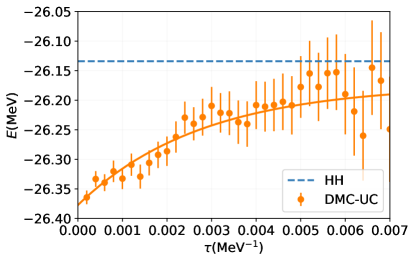
At first, we focus on the 4He nucleus, where we can carry out benchmark calculations between the AFDMC and HH methods. In the AV8P case, we estimate the uncertainty associated with using the replacement of Eq.(19) to include the isospin-dependent spin-orbit term in the AFDMC imaginary-time propagator by varying the parameter by 10% around its best value — we find for AV8P and AV8P+UIX cases, respectively. When the UIX potential is included in the Hamiltonian, we also vary by 10% — for both the AV6P+UIX and AV8P+UIX Hamiltonians. As a consequence, both the DMC-CP and DMC-UC errors for the AV8P, AV6P+UIX, and AV8P+UIX Hamiltonians are appreciably larger than for AV6P alone. Performing the unconstrained propagation improves the agreement between the AFDMC and HH methods, which is most apparent in the AV6P case, as it can be exactly included in the imaginary-time propagator. To better appreciate the bias introduced by the CP approximation, in Figure 2, we display the value of the ground-state energy of 4He during the unconstrained imaginary time propagation for the AV6P force. After about MeV-1, the DMC-UC ground-state energy agrees with the highly accurate HH value. We note that in contrast with the fixed node approximation employed in condensed-matter applications Foulkes et al. (2001), the constrained propagation breaks the variational principle Lynn et al. (2017). The value of the fit and its error are reported in Table 2. For the Hamiltonians that include spin-orbit NN interactions, the DMC-UC propagation produces energies about MeV less bound than the HH ones. However, the uncertainty associated with approximating the imaginary-time propagator as in Eq. (19) dominates this difference.
As already noted in Ref.Wiringa and Pieper (2002), both AV6P and AV8P alone underbind 4He by about MeV and MeV, respectively. In 4He, the attractive contribution of UIX is significantly more important than the repulsive , so overall UIX overbinds this nucleus by about MeV and MeV when used in combination with the AV6P and AV8P potentials, respectively. These findings are consistent with the fact that the full AV18 interaction is less attractive than both AV8P and AV6P in 4HeWiringa and Pieper (2002).
| Hamiltonian | VMC | DMC-CP | DMC-UC |
|---|---|---|---|
| AV6P | -51.9(1) | -101.9(2) | - |
| AV8P | -40.2(1) | -96(1) | - |
| AV6P+UIX | -45.9(2) | -108(8) | -113(9) |
| AV8P+UIX | -40.2(4) | -104(8) | -112(9) |
The ground-state energies of 16O obtained from the AV6P, AV8P, AV6P+UIX, and AV8P+UIX Hamiltonians are listed in Table 3. To account for isospin-dependent spin-orbit terms in the imaginary-time propagator, we take for AV8P alone and for AV8P+UIX. On the other hand, we find the optimal values for the AV6P+UIX and AV8P+UIX Hamiltonians to be and , respectively. By comparing the DMC-CP and VMC ground-state energies, it is clear how the imaginary-time diffusion significantly improves them, much more than for 4He. This improvement is mostly due to the fact that the linearized spin-isospin correlations of Eq.(13) violate the factorization theorem, and hence become less accurate as the number of nucleons increases. Due to their significant computational cost, we carry out DMC-UC calculations only for the Hamiltonians that include a 3N force, namely AV6P+UIX and AV8P+UIX. The unconstrained propagation lowers the energies by about MeV for both Hamiltonians, indicating again the need for more sophisticated variational wave functions than the ones used here. The sizable uncertainties in both the DMC-CP and DMC-UC results are dominated by the approximations made in the imaginary-time propagator to include spin-isospin dependent spin-orbit terms and cubic spin-isospin operators—see Eqs.(19) and (20).
For both AV6P+UIX and AV8P+UIX, 16O turns out to be underbound compared to experiment. This finding is consistent with the results obtained within the cluster variational Monte Carlo method Lonardoni et al. (2017), although the AV18+UIX Hamiltonian was employed in that work. It also aligns with the observation that AV18+UIX underbinds light nuclei with more than nucleons Pieper (2008); Carlson et al. (2015), as well as with infinite nuclear matter results Akmal et al. (1998); Lovato et al. (2011). Simply refitting the parameters and is unlikely to resolve the overbinding of 4He and underbinding in heavier systems. Following the approach outlined in Ref. Gnech et al. (2023), reducing the range of while increasing the magnitude of is likely to improve the agreement with experiments. To this end, in future work, we plan to replace the function with the shorter-range Wood-Saxon functions that define the shape of the core of the AV18 interaction.
III.2 Spatial distributions and radii
Within the AFDMC, expectation values of operators that do not commute with the Hamiltonian, such as the spatial and momentum distributions, are estimated at first order in perturbation theory as
| (29) |
Hence, in addition to controlling the fermion-sign problem, the accuracy of the variational state plays an important role to evaluate observables that do not commute with the Hamiltonian. In the following, we will present results for the single-nucleon density, which is defined as
| (30) |
Center of mass contaminations are automatically removed by , where is the center of mass coordinate of the nucleus Massella et al. (2020). In the above equation, we introduced the proton and neutron projector operators
| (31) |
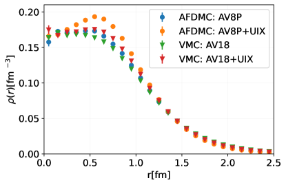
Figure 3 illustrates the AFDMC point-proton density of 4He as obtained from the AV8P and AV8P+UIX Hamiltonians. We compare the AFDMC results with VMC calculations carried out with the AV18 and AV18+UIX Hamiltonians Pieper et al. (2001); Pieper and Wiringa (2001). When NN forces only are included, we observe excellent agreement between the VMC and the AFDMC. On the other hand, the effect of the 3N potential appears to be stronger in AFDMC than in the VMC, as it enhances the point-proton density at around fm. The corresponding charge radii, listed in Table 4, are consistent with this behavior. The expectation value of the charge radius is derived from the point-proton radius using the relation Lonardoni et al. (2017, 2018)
| (32) |
where is the calculated point-proton radius, fm2 the proton radius Beringer et al. (2012), fm2 the neutron radius Beringer et al. (2012), and fm2 the Darwin-Foldy correction Friar et al. (1997).
Note that we neglect both the spin-orbit correction of Ref.Ong et al. (2010) and two-body terms in the charge operatorLovato et al. (2013).
Consistent with the ground-state energies of Table 2, the theoretical uncertainty of the AFDMC calculations accounts for the approximations made in the imaginary-time propagator.
| AV8P | AV8P+UIX | AV18 | AV18+UIX | Exp. |
| 1.69(4) | 1.64(6) | 1.734(3) | 1.665(3) | 1.676(3) |
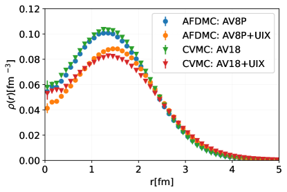
The AFDMC point-proton density of 16O computed using the AV8P and AV8P+UIX Hamiltonians is displayed in Figure 4. In this case, we compare the AFDMC results against the cluster variational Monte Carlo (CVMC) calculations carried out in Ref.Lonardoni et al. (2017). CVMC is a variational Monte Carlo method capable of computing nuclei with up to nucleons by utilizing a cluster expansion scheme for the spin-isospin dependent correlations present in the variational wave functions, considering up to five-body cluster terms. Thanks to this cluster expansion, there is no need to linearize the spin-dependent correlations as in Eq.(13). Hence, the CVMC variational wave functions are more accurate than those employed as a starting point for AFDMC calculations.
| AV8P | AV8P+UIX | AV18 | AV18+UIX | Exp. |
| 2.58(6) | 2.61(9) | 2.538(2) | 2.745(2) | 2.699(5) |
There is excellent agreement between AFDMC and CVMC results, both for Hamiltonians including NN only and for the full NN+3N case. However, it should be noted that the repulsion brought about by the 3N potential appears to be stronger in AFDMC than in CVMC, resulting in a more prominent depletion of the density at short distances. These differences are likely attributed to the fact that in the CVMC method, three-body correlations in the variational wave function are treated at first-order in perturbation theory. On the other hand, although the same approximation applies to the AFDMC variational state, in AFDMC, correlations induced by the 3N potential are accounted for by the imaginary-time propagator—albeit the commutator term of UIX is approximated as discussed in Eq.(20). This behavior is reflected in Table5, which shows the charge radius of 16O for the same Hamiltonians as discussed above. The 3N force, while being overall attractive, increases the charge radius by only about fm, primarily because of the repulsive term. However, it should be noted that these differences are much smaller than the uncertainties arising from using an approximated imaginary-time propagator to account for isospin-dependent spin-orbit terms and cubic spin-isospin operators.
III.3 Momentum distributions
Momentum distributions reflect features of both long- and short-distance nuclear dynamics and can provide useful insight into nuclear reactions, including inclusive and semi-inclusive electron and neutrino-nucleus scattering. The probability of finding a nucleon with momentum and isospin projection in the nuclear ground-state is proportional to the density
| (33) |
where is a vector in spin-isospin space.
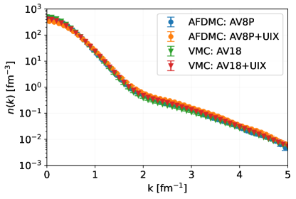
Figure 5 shows the AFDMC proton momentum distribution of 4He as obtained using the AV8P and AV8P+UIX interactions, compared with VMC calculations that use the AV18 and AV18+UIX combinations of NN and 3N potentials. All the curves are close to each other, both in the low- and high-momentum regions, and they all exhibit a large tail extending to high momenta. The presence of this tail is a consequence of the high-resolution nature of the Argonne family of interactions, which generate high-momentum components in the wave function. Note that the similarity renormalization group has recently proven to quantitatively reproduce the high-resolution distributions using evolved operators and low-resolution wave functions Tropiano et al. (2024). The 3N potential reduces the momentum distribution at low momenta and further increases its tail. Overall, this effect appears to be more significant in the AFDMC than in the VMC, consistent with what is observed in the single-nucleon spatial density displayed in Figure 3.
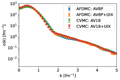
Similar considerations, including the presence of a high-momentum tail, can be made for the proton momentum distribution of 16O, displayed in Figure 6. The AFDMC calculations agree well with the CVMC results from Ref.Lonardoni et al. (2017), largely independent of the input Hamiltonian. The accuracy of the CVMC method in computing the momentum distribution is particularly high, given the rapid convergence of the cluster expansions. This behavior is consistent with the recent similarity renormalization group analysis from Ref. Tropiano et al. (2024), where keeping only two-body terms in the unitary transformation operator reproduces VMC results at the percent level.
III.4 Euclidean density responses
In this work, we focus on the isoscalar density transition operator, defined as
| (34) |
Besides the obvious exception of the missing proton projection operator, the isoscalar density transition operator bears close similarities to the time component of the one-body electromagnetic current operator, which defines the electromagnetic longitudinal response of the nucleus. The latter quantity is critical for determining inclusive electron- and neutrino-nucleus scattering cross sections Carlson et al. (2002), and to identify potential explicit quark and gluons effects in nuclear structure Jourdan (1996).
The corresponding response function is defined as
| (35) |
where and denote the momentum and energy transfer, respectively. In the above equation, and are the initial and final nuclear states with energies and , respectively. In order to avoid computing all transitions induced by the current operator — which is impractical except for very light nuclear systems Shen et al. (2012); Golak et al. (2018) — similar to previous Green’s function Monte Carlo calculations, we infer properties of the response function from its Laplace transform Carlson and Schiavilla (1992); Carlson et al. (2002)
| (36) |
Leveraging the completeness of the final states of the reaction, the Euclidean response can be expressed as a ground-state expectation value:
| (37) |
where is the nuclear Hamiltonian.
Within the AFDMC, we evaluate the above expectation value employing the same imaginary-time propagation we use for finding the ground-state of the system. Since the isoscalar density transition operator defined in Eq. (34) does not encompass spin-isospin operators, we can readily express the Euclidean response as
| (38) |
where denotes the spatial coordinate of the -th nucleon at imaginary time .
In this work, as commonly done in previous Green’s function Monte Carlo applications Lovato et al. (2013, 2020), we approximate the ground-state with the variational wave function . While this procedure is accurate for 4He, its applicability to 16O is more questionable, owing to the limitations inherent to using linearized spin-isospin dependent correlations. In future works, we plan on correcting these variational estimates within perturbation theory, as in Eq. 29. For this reason, here we do not attempt inverting the Laplace transform either using Maximum Entropy Bryan (1990); Jarrell and Gubernatis (1996) or the recently developed machine-learning inversion protocols Raghavan et al. (2021); Raghavan and Lovato (2023). Rather, we focus on the computational feasibility of this quantity within the AFDMC, which can tackle larger nuclei than the GFMC, previously applied only up to 12C.
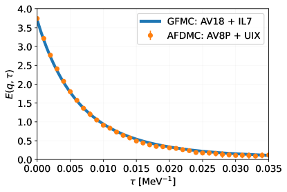
In Figure 7, we compare the 4He Euclidean isoscalar density response function computed with the AFDMC and GFMC methods using as input the AV8P+UIX and AV18+IL7 Hamiltonians, respectively. Despite the different NN and 3N forces, the Euclidean response functions are close to each other up to the largest value of imaginary time we consider, MeV-1. This agreement is reassuring, as it corroborates both the AFDMC implementation of the Euclidean response-function calculation and the accuracy of the method, despite somewhat different input Hamiltonians.
The 4He Euclidean isoscalar density response function shown in Figure 7 has been computed by carrying out DMC-UC propagations to remove the bias associated with the fermion sign problem. However, when tackling larger nuclei such as 16O, the unconstrained propagation yields sizable statistical fluctuations in the Euclidean response, primarily arising from the somewhat oversimplified correlation operator of Eq.(13). In Figure 8, we display the Euclidean isoscalar density response function of 16He at MeV corresponding to the AV8P+UIX Hamiltonian. The DMC-UC results, denoted by the blue solid circles, start exhibiting large statistical fluctuations after around MeV-1. On the other hand, employing the same DMC-CP approximation used in ground-state calculations dramatically reduces the noise, making it possible to reach much larger imaginary times. In the region MeV-1, the DMC-CP and DMC-UC responses are consistent within statistical error, suggesting that the constrained-path approximation does not significantly bias the Monte Carlo estimates. Note that carrying out the DMC-UC calculations required about ten million CPU hours on Intel-KNL to keep the statistical noise under control, while the DMC-CP calculations are significantly cheaper. In the future, we plan to explore the contour-deformation techniques developed in Ref. Kanwar et al. (2024) to reduce the statistical uncertainty plaguing the unconstrained results.
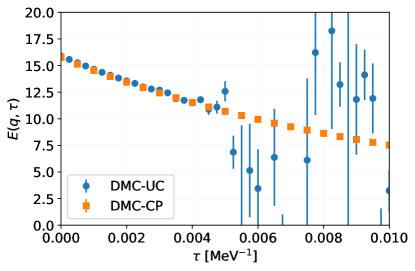
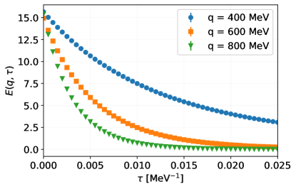
Figure 9 displays the Euclidean isoscalar density response function at momentum transfers of MeV, MeV, and MeV, computed within the DMC-CP approximation using the AV8P+UIX Hamiltonian. Increasing the momentum transfer shifts the position of the quasi-elastic peak to higher energy transfers, thereby suppressing the Euclidean responses at large imaginary times. Additionally, the elastic contribution — corresponding to in Eq. (35) — is much smaller at MeV and MeV than at MeV, further contributing to the reduction of the Euclidean responses at large . All these features are observed in the AFDMC curves, once again corroborating the accuracy of the novel methodology we developed.
IV Conclusions
We carried out AFDMC calculations of the ground-state static and dynamic properties of 4He and 16O using high-resolution phenomenological Hamiltonians from the Argonne family. For the 4He nucleus, we performed detailed benchmarks with the highly accurate hyperspherical harmonics method. This comparison corroborated the reliability of the AFDMC method, particularly the approximations made to treat isospin-dependent spin-orbit terms and cubic spin-isospin operators in the imaginary-time propagator. Nevertheless, these approximations contribute significantly to the uncertainties in our AFDMC results. To reduce them, we are currently working on a Restricted Boltzmann Machine representation of the imaginary-time propagator Rrapaj and Roggero (2021), which is showing promising results and will be the subject of a future publication. Additionally, the AFDMC ground-state energies are affected by a non-negligible sign problem, particularly for 16O. To mitigate this issue, we plan to employ more accurate variational wave functions than those used here, leveraging neural-network quantum states Adams et al. (2021); Lovato et al. (2022a).
Our analysis confirms the inadequacy of both AV6P+UIX and AV8P+UIX Hamiltonians in describing simultaneously the ground-state properties of 4He and 16O nuclei. This finding is consistent with FHNC/SOC calculations of the energy per particle of isospin-symmetric nuclear matter at saturation density Akmal et al. (1998); Lovato et al. (2011), which indicate a binding energy about MeV lower than the empirical value. A potential solution to this problem, inspired by chiral effective field theory, involves replacing the squared Yukawa function in the repulsive 3N component with a shorter-ranged parameterization, consistent with the Wood-Saxon functions defining the core shape of the AV18 interaction. To this end, we plan to incorporate these shorter-ranged 3N forces in a simultaneous AFDMC/GFMC analysis of 4He, 12C, and 16O nuclei, alongside the neutron-matter equation of state. Our objective is to identify a high-resolution Hamiltonian capable of accurately describing nuclei up to 16O, as well as the high-density neutron-star matter found in the inner core of neutron stars. An alternative possibility is to include relativistic boost corrections in the Hamiltonian Forest et al. (1995a), which are known to change the strength of the 3N interaction in light nuclei Forest et al. (1995b); Yang and Zhao (2022) and might help reproducing saturation properties of isospin-symmetric nuclear matter Akmal et al. (1998); Yang and Zhao (2024).
We established a computational protocol for carrying out AFDMC calculations of the Euclidean isoscalar density response function of atomic nuclei, validating it against GFMC results of 4He. Treating 16O results in significantly higher statistical noise, which we controlled by employing the same constrained-path approximation used for computing the ground-state energy of the system. To achieve fully unbiased calculations, we intend to explore contour deformation techniques successfully applied to GFMC calculations of the isoscalar density response of the deuteron in Ref. Kanwar et al. (2024). With the algorithmic foundations laid, we are now well-positioned to compute the electroweak response functions of 16O, including both one- and two-body current contributions, which are essential for evaluating inclusive electron and neutrino scattering cross-sections.
The calculations conducted in this work will provide important inputs to the ACHILLES neutrino event generator Isaacson et al. (2021, 2023). Specifically, we will supply ACHILLES with AFDMC samples of three-dimensional positions of protons and neutrons in the 16O nucleus. These samples fully encode correlation effects and, by definition, reproduce the one- and two-body isospin dependent spatial density distributions. The significance of including correlations in the propagation of the scattered particle throughout the nucleus will be examined by comparing against nuclear transparency data Isaacson et al. (2021) and other relevant observables. Additionally, the momentum distributions computed in this study will serve as a normalization test for the single-nucleon spectral functions used in ACHILLES to compute the elementary vertex.
V Acknowledgements
We thank R. B. Wiringa for providing us with the phase shifts of the Argonne potentials and for critically reading the manuscript. We are also grateful to R. Schiavilla for the invaluable suggestions provided during the initial phase of this study. This work was supported by the U.S. Department of Energy (DOE), Office of Science, Office of Nuclear Physics under contract number DE-AC02-06CH11357 (A.L.) and by the SciDAC-NUCLEI (A.L., ) and SciDAC-NeuCol (A.L. and N.R.) projects. A.L. is also supported by DOE Early Career Research Program awards. A.G. acknowledges support from the DOE Topical Collaboration “Nuclear Theory for New Physics,” award No. DE-SC0023663 and Jefferson Lab that is supported by the U.S. Department of Energy, Office of Nuclear Science, under Contracts No. DE-AC05-06OR23177. Quantum Monte Carlo calculations were performed on the parallel computers of the Laboratory Computing Resource Center, Argonne National Laboratory, the computers of the Argonne Leadership Computing Facility via ALCC and INCITE grants. Hyperspherical Harmonic calculations were performed at NERSC, a U.S. Department of Energy Office of Science User Facility located at Lawrence Berkeley National Laboratory, operated under Contract No. DE-AC02-05CH11231 using NERSC award NP-ERCAP0023221.
References
- Weinberg (1990) Steven Weinberg, “Nuclear forces from chiral Lagrangians,” Phys. Lett. B251, 288–292 (1990).
- Weinberg (1991) Steven Weinberg, “Effective chiral Lagrangians for nucleon - pion interactions and nuclear forces,” Nucl. Phys. B363, 3–18 (1991).
- Epelbaum et al. (2009) Evgeny Epelbaum, Hans-Werner Hammer, and Ulf-G. Meissner, “Modern Theory of Nuclear Forces,” Rev. Mod. Phys. 81, 1773–1825 (2009), arXiv:0811.1338 [nucl-th] .
- Machleidt and Entem (2011) R. Machleidt and D. R. Entem, “Chiral effective field theory and nuclear forces,” Phys. Rept. 503, 1–75 (2011), arXiv:1105.2919 [nucl-th] .
- Reinert et al. (2018) P. Reinert, H. Krebs, and E. Epelbaum, “Semilocal momentum-space regularized chiral two-nucleon potentials up to fifth order,” Eur. Phys. J. A54, 86 (2018), arXiv:1711.08821 [nucl-th] .
- Entem et al. (2017) D. R. Entem, R. Machleidt, and Y. Nosyk, “High-quality two-nucleon potentials up to fifth order of the chiral expansion,” Phys. Rev. C96, 024004 (2017), arXiv:1703.05454 [nucl-th] .
- Carbone et al. (2013) Arianna Carbone, Andrea Cipollone, Carlo Barbieri, Arnau Rios, and Artur Polls, “Self-consistent Green’s functions formalism with three-body interactions,” Phys. Rev. C88, 054326 (2013), arXiv:1310.3688 [nucl-th] .
- Barrett et al. (2013) Bruce R. Barrett, Petr Navratil, and James P. Vary, “Ab initio no core shell model,” Prog. Part. Nucl. Phys. 69, 131–181 (2013).
- Hagen et al. (2014) G. Hagen, T. Papenbrock, M. Hjorth-Jensen, and D. J. Dean, “Coupled-cluster computations of atomic nuclei,” Rept. Prog. Phys. 77, 096302 (2014), arXiv:1312.7872 [nucl-th] .
- Carlson et al. (2015) J. Carlson, S. Gandolfi, F. Pederiva, Steven C. Pieper, R. Schiavilla, K. E. Schmidt, and R. B. Wiringa, “Quantum Monte Carlo methods for nuclear physics,” Rev. Mod. Phys. 87, 1067 (2015), arXiv:1412.3081 [nucl-th] .
- Hergert et al. (2016) H. Hergert, S. K. Bogner, T. D. Morris, A. Schwenk, and K. Tsukiyama, “The In-Medium Similarity Renormalization Group: A Novel Ab Initio Method for Nuclei,” Phys. Rept. 621, 165–222 (2016), arXiv:1512.06956 [nucl-th] .
- Lynn et al. (2019) J. E. Lynn, I. Tews, S. Gandolfi, and A. Lovato, “Quantum Monte Carlo Methods in Nuclear Physics: Recent Advances,” Ann. Rev. Nucl. Part. Sci. 69, 279–305 (2019), arXiv:1901.04868 [nucl-th] .
- Hu et al. (2022) Baishan Hu et al., “Ab initio predictions link the neutron skin of 208Pb to nuclear forces,” Nature Phys. 18, 1196–1200 (2022), arXiv:2112.01125 [nucl-th] .
- Malbrunot-Ettenauer et al. (2022) S. Malbrunot-Ettenauer et al., “Nuclear Charge Radii of the Nickel Isotopes 58-68,70Ni,” Phys. Rev. Lett. 128, 022502 (2022), arXiv:2112.03382 [nucl-ex] .
- Lechner et al. (2023) S. Lechner et al., “Electromagnetic moments of the antimony isotopes 112-133Sb,” Phys. Lett. B 847, 138278 (2023), arXiv:2311.01110 [nucl-ex] .
- Gysbers et al. (2019) P. Gysbers et al., “Discrepancy between experimental and theoretical -decay rates resolved from first principles,” Nature Phys. 15, 428–431 (2019), arXiv:1903.00047 [nucl-th] .
- Ekström et al. (2013) A. Ekström et al., “Optimized Chiral Nucleon-Nucleon Interaction at Next-to-Next-to-Leading Order,” Phys. Rev. Lett. 110, 192502 (2013), arXiv:1303.4674 [nucl-th] .
- Ekström et al. (2015) A. Ekström, G. R. Jansen, K. A. Wendt, G. Hagen, T. Papenbrock, B. D. Carlsson, C. Forssén, M. Hjorth-Jensen, P. Navrátil, and W. Nazarewicz, “Accurate nuclear radii and binding energies from a chiral interaction,” Phys. Rev. C 91, 051301 (2015), arXiv:1502.04682 [nucl-th] .
- Jiang et al. (2020) W. G. Jiang, A. Ekström, C. Forssén, G. Hagen, G. R. Jansen, and T. Papenbrock, “Accurate bulk properties of nuclei from to from potentials with isobars,” Phys. Rev. C 102, 054301 (2020), arXiv:2006.16774 [nucl-th] .
- Lu et al. (2019) Bing-Nan Lu, Ning Li, Serdar Elhatisari, Dean Lee, Evgeny Epelbaum, and Ulf-G. Meißner, “Essential elements for nuclear binding,” Phys. Lett. B 797, 134863 (2019), arXiv:1812.10928 [nucl-th] .
- Gattobigio et al. (2019) Mario Gattobigio, Alejandro Kievsky, and Michele Viviani, “Embedding nuclear physics inside the unitary-limit window,” Phys. Rev. C 100, 034004 (2019), arXiv:1903.08900 [nucl-th] .
- Kievsky et al. (2021) A. Kievsky, L. Girlanda, M. Gattobigio, and M. Viviani, “Efimov Physics and Connections to Nuclear Physics,” Ann. Rev. Nucl. Part. Sci. 71, 465–490 (2021), arXiv:2102.13504 [nucl-th] .
- Schiavilla et al. (2021) R. Schiavilla, L. Girlanda, A. Gnech, A. Kievsky, A. Lovato, L. E. Marcucci, M. Piarulli, and M. Viviani, “Two- and three-nucleon contact interactions and ground-state energies of light- and medium-mass nuclei,” Phys. Rev. C 103, 054003 (2021), arXiv:2102.02327 [nucl-th] .
- Lovato et al. (2022a) Alessandro Lovato, Corey Adams, Giuseppe Carleo, and Noemi Rocco, “Hidden-nucleons neural-network quantum states for the nuclear many-body problem,” Phys. Rev. Res. 4, 043178 (2022a), arXiv:2206.10021 [nucl-th] .
- Gnech et al. (2023) A. Gnech, B. Fore, and A. Lovato, “Distilling the essential elements of nuclear binding via neural-network quantum states,” (2023), arXiv:2308.16266 [nucl-th] .
- Lovato et al. (2022b) A. Lovato, I. Bombaci, D. Logoteta, M. Piarulli, and R. B. Wiringa, “Benchmark calculations of infinite neutron matter with realistic two- and three-nucleon potentials,” Phys. Rev. C 105, 055808 (2022b), arXiv:2202.10293 [nucl-th] .
- Piarulli et al. (2018) M. Piarulli et al., “Light-nuclei spectra from chiral dynamics,” Phys. Rev. Lett. 120, 052503 (2018), arXiv:1707.02883 [nucl-th] .
- Baroni et al. (2018) A. Baroni et al., “Local chiral interactions, the tritium Gamow-Teller matrix element, and the three-nucleon contact term,” Phys. Rev. C 98, 044003 (2018), arXiv:1806.10245 [nucl-th] .
- Lovato et al. (2012) Alessandro Lovato, Omar Benhar, Stefano Fantoni, and Kevin E. Schmidt, “Comparative study of three-nucleon potentials in nuclear matter,” Phys. Rev. C 85, 024003 (2012), arXiv:1109.5489 [nucl-th] .
- Hüther et al. (2020) Thomas Hüther, Klaus Vobig, Kai Hebeler, Ruprecht Machleidt, and Robert Roth, “Family of Chiral Two- plus Three-Nucleon Interactions for Accurate Nuclear Structure Studies,” Phys. Lett. B 808, 135651 (2020), arXiv:1911.04955 [nucl-th] .
- Sammarruca and Millerson (2020) Francesca Sammarruca and Randy Millerson, “Exploring the relationship between nuclear matter and finite nuclei with chiral two- and three-nucleon forces,” Phys. Rev. C 102, 034313 (2020), arXiv:2005.01958 [nucl-th] .
- Wiringa et al. (1995) Robert B. Wiringa, V. G. J. Stoks, and R. Schiavilla, “An Accurate nucleon-nucleon potential with charge independence breaking,” Phys. Rev. C 51, 38–51 (1995), arXiv:nucl-th/9408016 .
- Benhar (2021) Omar Benhar, “Scale dependence of the nucleon–nucleon potential,” Int. J. Mod. Phys. E 30, 2130009 (2021).
- Schmidt et al. (2020) A. Schmidt et al. (CLAS), “Probing the core of the strong nuclear interaction,” Nature 578, 540–544 (2020), arXiv:2004.11221 [nucl-ex] .
- Pieper (2008) Steven C. Pieper, “The Illinois Extension to the Fujita-Miyazawa Three-Nucleon Force,” AIP Conf. Proc. 1011, 143–152 (2008).
- Maris et al. (2013) Pieter Maris, James P. Vary, S. Gandolfi, J. Carlson, and Steven C. Pieper, “Properties of trapped neutrons interacting with realistic nuclear Hamiltonians,” Phys. Rev. C 87, 054318 (2013), arXiv:1302.2089 [nucl-th] .
- Pieper et al. (2001) Steven C. Pieper, V. R. Pandharipande, Robert B. Wiringa, and J. Carlson, “Realistic models of pion exchange three nucleon interactions,” Phys. Rev. C 64, 014001 (2001), arXiv:nucl-th/0102004 .
- Wiringa and Pieper (2002) Robert B. Wiringa and Steven C. Pieper, “Evolution of nuclear spectra with nuclear forces,” Phys. Rev. Lett. 89, 182501 (2002), arXiv:nucl-th/0207050 .
- Pudliner et al. (1995) B. S. Pudliner, V. R. Pandharipande, J. Carlson, and Robert B. Wiringa, “Quantum Monte Carlo calculations of A = 6 nuclei,” Phys. Rev. Lett. 74, 4396–4399 (1995), arXiv:nucl-th/9502031 .
- Kievsky et al. (2008) A. Kievsky, S. Rosati, M. Viviani, L. E. Marcucci, and L. Girlanda, “A High-precision variational approach to three- and four-nucleon bound and zero-energy scattering states,” J. Phys. G 35, 063101 (2008), arXiv:0805.4688 [nucl-th] .
- Marcucci et al. (2020) L. E. Marcucci, J. Dohet-Eraly, L. Girlanda, A. Gnech, A. Kievsky, and M. Viviani, “The Hyperspherical Harmonics method: a tool for testing and improving nuclear interaction models,” Front. in Phys. 8, 69 (2020), arXiv:1912.09751 [nucl-th] .
- Kamada et al. (2001) H. Kamada et al., “Benchmark test calculation of a four nucleon bound state,” Phys. Rev. C 64, 044001 (2001), arXiv:nucl-th/0104057 .
- Hagen et al. (2007) G. Hagen, T. Papenbrock, D. J. Dean, A. Schwenk, A. Nogga, M. Wloch, and P. Piecuch, “Coupled-cluster theory for three-body Hamiltonians,” Phys. Rev. C 76, 034302 (2007), arXiv:0704.2854 [nucl-th] .
- Tichai et al. (2020) Alexander Tichai, Robert Roth, and Thomas Duguet, “Many-body perturbation theories for finite nuclei,” Front. in Phys. 8, 164 (2020), arXiv:2001.10433 [nucl-th] .
- Baldo et al. (2012) M. Baldo, A. Polls, A. Rios, H. J. Schulze, and I. Vidana, “Comparative study of neutron and nuclear matter with simplified Argonne nucleon-nucleon potentials,” Phys. Rev. C 86, 064001 (2012), arXiv:1207.6314 [nucl-th] .
- Piarulli et al. (2020) M. Piarulli, I. Bombaci, D. Logoteta, A. Lovato, and R. B. Wiringa, “Benchmark calculations of pure neutron matter with realistic nucleon-nucleon interactions,” Phys. Rev. C 101, 045801 (2020), arXiv:1908.04426 [nucl-th] .
- Stoks et al. (1993) V. G. J. Stoks, R. A. M. Klomp, M. C. M. Rentmeester, and J. J. de Swart, “Partial wave analaysis of all nucleon-nucleon scattering data below 350-MeV,” Phys. Rev. C 48, 792–815 (1993).
- Workman et al. (2016) Ron L. Workman, William J. Briscoe, and Igor I. Strakovsky, “Partial-Wave Analysis of Nucleon-Nucleon Elastic Scattering Data,” Phys. Rev. C 94, 065203 (2016), arXiv:1609.01741 [nucl-th] .
- Fujita and Miyazawa (1957) J. Fujita and H. Miyazawa, “Pion Theory of Three-Body Forces,” Prog. Theor. Phys. 17, 360–365 (1957).
- Coon et al. (1979) S. A. Coon, M. D. Scadron, P. C. McNamee, B. R. Barrett, D. W. E. Blatt, and B. H. J. McKellar, “The Two Pion Exchange, Three Nucleon Potential and Nuclear Matter,” Nucl. Phys. A 317, 242–278 (1979).
- Coelho et al. (1983) H. T. Coelho, T. K. Das, and M. R. Robilotta, “TWO PION EXCHANGE THREE NUCLEON FORCE AND THE H-3 AND HE-3 NUCLEI,” Phys. Rev. C 28, 1812–1828 (1983).
- Lagaris and Pandharipande (1981) I. E. Lagaris and V. R. Pandharipande, “Variational Calculations of Realistic Models of Nuclear Matter,” Nucl. Phys. A 359, 349–364 (1981).
- Schmidt and Fantoni (1999) K. E. Schmidt and S. Fantoni, “A quantum Monte Carlo method for nucleon systems,” Phys. Lett. B 446, 99–103 (1999).
- Contessi et al. (2017) L. Contessi, A. Lovato, F. Pederiva, A. Roggero, J. Kirscher, and U. van Kolck, “Ground-state properties of 4He and 16O extrapolated from lattice QCD with pionless EFT,” Phys. Lett. B 772, 839–848 (2017), arXiv:1701.06516 [nucl-th] .
- Gandolfi et al. (2014) S. Gandolfi, A. Lovato, J. Carlson, and Kevin E. Schmidt, “From the lightest nuclei to the equation of state of asymmetric nuclear matter with realistic nuclear interactions,” Phys. Rev. C 90, 061306 (2014), arXiv:1406.3388 [nucl-th] .
- Gandolfi et al. (2020) Stefano Gandolfi, Diego Lonardoni, Alessandro Lovato, and Maria Piarulli, “Atomic nuclei from quantum Monte Carlo calculations with chiral EFT interactions,” Front. in Phys. 8, 117 (2020), arXiv:2001.01374 [nucl-th] .
- Lonardoni et al. (2018) D. Lonardoni, S. Gandolfi, J. E. Lynn, C. Petrie, J. Carlson, K. E. Schmidt, and A. Schwenk, “Auxiliary field diffusion Monte Carlo calculations of light and medium-mass nuclei with local chiral interactions,” Phys. Rev. C 97, 044318 (2018), arXiv:1802.08932 [nucl-th] .
- Toulouse and Umrigar (2007) J. Toulouse and C. J. Umrigar, “Optimization of quantum Monte Carlo wave functions by energy minimization,” J. Chem. Phys. 126, 084102 (2007), physics/0701039 .
- Adams et al. (2021) Corey Adams, Giuseppe Carleo, Alessandro Lovato, and Noemi Rocco, “Variational Monte Carlo Calculations of A4 Nuclei with an Artificial Neural-Network Correlator Ansatz,” Phys. Rev. Lett. 127, 022502 (2021), arXiv:2007.14282 [nucl-th] .
- Gnech et al. (2022) Alex Gnech, Corey Adams, Nicholas Brawand, Giuseppe Carleo, Alessandro Lovato, and Noemi Rocco, “Nuclei with up to nucleons with artificial neural network wave functions,” Few Body Syst. 63, 7 (2022), arXiv:2108.06836 [nucl-th] .
- Zhang et al. (1997) Shiwei Zhang, J. Carlson, and J. E. Gubernatis, “A Constrained path Monte Carlo method for fermion ground states,” Phys. Rev. B 55, 7464 (1997), arXiv:cond-mat/9607062 .
- Zhang and Krakauer (2003) Shiwei Zhang and Henry Krakauer, “Quantum Monte Carlo method using phase-free random walks with Slater determinants,” Phys. Rev. Lett. 90, 136401 (2003), arXiv:cond-mat/0208340 .
- Wiringa et al. (2000) Robert B. Wiringa, Steven C. Pieper, J. Carlson, and V. R. Pandharipande, “Quantum Monte Carlo calculations of A = 8 nuclei,” Phys. Rev. C 62, 014001 (2000), arXiv:nucl-th/0002022 .
- Pederiva et al. (2004) Francesco Pederiva, A. Sarsa, K. E. Schmidt, and S. Fantoni, “Auxiliary field diffusion Monte Carlo calculation of ground state properties of neutron drops,” Nucl. Phys. A 742, 255–268 (2004), arXiv:nucl-th/0403069 .
- Pudliner et al. (1997) B. S. Pudliner, V. R. Pandharipande, J. Carlson, Steven C. Pieper, and Robert B. Wiringa, “Quantum Monte Carlo calculations of nuclei with A = 7,” Phys. Rev. C 56, 1720–1750 (1997), arXiv:nucl-th/9705009 .
- Rrapaj and Roggero (2021) Ermal Rrapaj and Alessandro Roggero, “Exact representations of many-body interactions with restricted-Boltzmann-machine neural networks,” Phys. Rev. E 103, 013302 (2021), arXiv:2005.03568 [nucl-th] .
- Viviani et al. (2005) M. Viviani, A. Kievsky, and S. Rosati, “Calculation of the alpha-particle ground state within the hyperspherical harmonic basis,” Phys. Rev. C 71, 024006 (2005), arXiv:nucl-th/0408019 .
- Gnech et al. (2020) Alex Gnech, Michele Viviani, and Laura Elisa Marcucci, “Calculation of the 6Li ground state within the hyperspherical harmonic basis,” Phys. Rev. C 102, 014001 (2020), arXiv:2004.05814 [nucl-th] .
- Foulkes et al. (2001) W. M. Foulkes, L. Mitas, R. J. Needs, and G. Rajagopal, “Quantum Monte Carlo simulations of solids,” Reviews of Modern Physics 73, 33–83 (2001).
- Lynn et al. (2017) J. E. Lynn, I. Tews, J. Carlson, S. Gandolfi, A. Gezerlis, K. E. Schmidt, and A. Schwenk, “Quantum Monte Carlo calculations of light nuclei with local chiral two- and three-nucleon interactions,” Phys. Rev. C 96, 054007 (2017), arXiv:1706.07668 [nucl-th] .
- Lonardoni et al. (2017) D. Lonardoni, A. Lovato, Steven C. Pieper, and R. B. Wiringa, “Variational calculation of the ground state of closed-shell nuclei up to ,” Phys. Rev. C 96, 024326 (2017), arXiv:1705.04337 [nucl-th] .
- Akmal et al. (1998) A. Akmal, V. R. Pandharipande, and D. G. Ravenhall, “The Equation of state of nucleon matter and neutron star structure,” Phys. Rev. C 58, 1804–1828 (1998), arXiv:nucl-th/9804027 .
- Lovato et al. (2011) Alessandro Lovato, Omar Benhar, Stefano Fantoni, Alexey Yu. Illarionov, and Kevin E. Schmidt, “Density-dependent nucleon-nucleon interaction from three-nucleon forces,” Phys. Rev. C 83, 054003 (2011), arXiv:1011.3784 [nucl-th] .
- Massella et al. (2020) P. Massella, F. Barranco, D. Lonardoni, A. Lovato, F. Pederiva, and E. Vigezzi, “Exact restoration of Galilei invariance in density functional calculations with quantum Monte Carlo,” J. Phys. G 47, 035105 (2020), arXiv:1808.00518 [nucl-th] .
- Pieper and Wiringa (2001) Steven C. Pieper and Robert B. Wiringa, “Quantum Monte Carlo calculations of light nuclei,” Ann. Rev. Nucl. Part. Sci. 51, 53–90 (2001), arXiv:nucl-th/0103005 .
- Beringer et al. (2012) J. Beringer et al. (Particle Data Group), “Review of Particle Physics (RPP),” Phys. Rev. D 86, 010001 (2012).
- Friar et al. (1997) James Lewis Friar, J. Martorell, and D. W. L. Sprung, “Nuclear sizes and the isotope shift,” Phys. Rev. A 56, 4579–4586 (1997), arXiv:nucl-th/9707016 .
- Ong et al. (2010) A. Ong, J. C. Berengut, and V. V. Flambaum, “The Effect of spin-orbit nuclear charge density corrections due to the anomalous magnetic moment on halonuclei,” Phys. Rev. C 82, 014320 (2010), arXiv:1006.5508 [nucl-th] .
- Lovato et al. (2013) A. Lovato, S. Gandolfi, Ralph Butler, J. Carlson, Ewing Lusk, Steven C. Pieper, and R. Schiavilla, “Charge Form Factor and Sum Rules of Electromagnetic Response Functions in ,” Phys. Rev. Lett. 111, 092501 (2013), arXiv:1305.6959 [nucl-th] .
- Tropiano et al. (2024) A. J. Tropiano, S. K. Bogner, R. J. Furnstahl, M. A. Hisham, A. Lovato, and R. B. Wiringa, “High-resolution momentum distributions from low-resolution wave functions,” Phys. Lett. B 852, 138591 (2024), arXiv:2402.00634 [nucl-th] .
- Carlson et al. (2002) J. Carlson, J. Jourdan, R. Schiavilla, and I. Sick, “Longitudinal and transverse quasielastic response functions of light nuclei,” Phys. Rev. C 65, 024002 (2002), arXiv:nucl-th/0106047 .
- Jourdan (1996) J. Jourdan, “Quasielastic response functions: The Coulomb sum revisited,” Nucl. Phys. A 603, 117–160 (1996).
- Shen et al. (2012) G. Shen, L. E. Marcucci, J. Carlson, S. Gandolfi, and R. Schiavilla, “Inclusive neutrino scattering off deuteron from threshold to GeV energies,” Phys. Rev. C 86, 035503 (2012), arXiv:1205.4337 [nucl-th] .
- Golak et al. (2018) J. Golak, R. Skibiński, K. Topolnicki, H. Witała, A. Grassi, H. Kamada, and L. E. Marcucci, “Momentum space treatment of inclusive neutrino scattering off the deuteron and trinucleons,” Phys. Rev. C 98, 015501 (2018), arXiv:1805.00103 [nucl-th] .
- Carlson and Schiavilla (1992) J. Carlson and R. Schiavilla, “Euclidean proton response in light nuclei,” Phys. Rev. Lett. 68, 3682–3685 (1992).
- Lovato et al. (2020) A. Lovato, J. Carlson, S. Gandolfi, N. Rocco, and R. Schiavilla, “Ab initio study of and inclusive scattering in 12C: confronting the MiniBooNE and T2K CCQE data,” Phys. Rev. X 10, 031068 (2020), arXiv:2003.07710 [nucl-th] .
- Bryan (1990) R.K. Bryan, “Maximum entropy analysis of oversampled data problems,” European Biophysics Journal 18, 165–174 (1990).
- Jarrell and Gubernatis (1996) Mark Jarrell and J.E. Gubernatis, “Bayesian inference and the analytic continuation of imaginary-time quantum monte carlo data,” Physics Reports 269, 133 – 195 (1996).
- Raghavan et al. (2021) Krishnan Raghavan, Prasanna Balaprakash, Alessandro Lovato, Noemi Rocco, and Stefan M. Wild, “Machine learning-based inversion of nuclear responses,” Phys. Rev. C 103, 035502 (2021), arXiv:2010.12703 [nucl-th] .
- Raghavan and Lovato (2023) K. Raghavan and A. Lovato, “Uncertainty Quantification-Enabled Inversion of Nuclear Euclidean Responses,” (2023), arXiv:2310.18756 [nucl-th] .
- Kanwar et al. (2024) Gurtej Kanwar, Alessandro Lovato, Noemi Rocco, and Michael Wagman, “Mitigating Green’s function Monte Carlo signal-to-noise problems using contour deformations,” Phys. Rev. C 109, 034317 (2024), arXiv:2304.03229 [nucl-th] .
- Forest et al. (1995a) J. L. Forest, V. R. Pandharipande, and James Lewis Friar, “Relativistic nuclear Hamiltonians,” Phys. Rev. C 52, 568–575 (1995a).
- Forest et al. (1995b) J. L. Forest, V. R. Pandharipande, J. Carlson, and R. Schiavilla, “Variational Monte Carlo calculations of H-3 and He-4 with a relativistic Hamiltonian,” Phys. Rev. C 52, 576–577 (1995b).
- Yang and Zhao (2022) Y. L. Yang and P. W. Zhao, “A consistent description of the relativistic effects and three-body interactions in atomic nuclei,” Phys. Lett. B 835, 137587 (2022), arXiv:2206.13208 [nucl-th] .
- Yang and Zhao (2024) Y. L. Yang and P. W. Zhao, “Reconciling light nuclei and nuclear matter: relativistic calculations,” (2024), arXiv:2405.04203 [nucl-th] .
- Isaacson et al. (2021) Joshua Isaacson, William I. Jay, Alessandro Lovato, Pedro A. N. Machado, and Noemi Rocco, “New approach to intranuclear cascades with quantum Monte Carlo configurations,” Phys. Rev. C 103, 015502 (2021), arXiv:2007.15570 [hep-ph] .
- Isaacson et al. (2023) Joshua Isaacson, William I. Jay, Alessandro Lovato, Pedro A. N. Machado, and Noemi Rocco, “Introducing a novel event generator for electron-nucleus and neutrino-nucleus scattering,” Phys. Rev. D 107, 033007 (2023), arXiv:2205.06378 [hep-ph] .