SNF-ROM: Projection-based nonlinear reduced order modeling with smooth neural fields

Abstract

Reduced order modeling lowers the computational cost of solving PDEs by learning a low-order spatial representation from data and dynamically evolving these representations using manifold projections of the governing equations. While commonly used, linear subspace reduced-order models (ROMs) are often suboptimal for problems with a slow decay of Kolmogorov $n$-width, such as advection-dominated fluid flows at high Reynolds numbers. There has been a growing interest in nonlinear ROMs that use state-of-the-art representation learning techniques to accurately capture such phenomena with fewer degrees of freedom. We propose smooth neural field ROM (SNF-ROM), a nonlinear reduced modeling framework that combines grid-free reduced representations with Galerkin projection. The SNF-ROM architecture constrains the learned ROM trajectories to a smoothly varying path, which proves beneficial in the dynamics evaluation when the reduced manifold is traversed in accordance with the governing PDEs. Furthermore, we devise robust regularization schemes to ensure the learned neural fields are smooth and differentiable. This allows us to compute physics-based dynamics of the reduced system nonintrusively with automatic differentiation and evolve the reduced system with classical time-integrators. SNF-ROM leads to fast offline training as well as enhanced accuracy and stability during the online dynamics evaluation. We demonstrate the efficacy of SNF-ROM on a range of advection-dominated linear and nonlinear PDE problems where we consistently outperform state-of-the-art ROMs.

[inst1] organization=Mechanical Engineering, Carnegie Mellon University, addressline=5000 Forbes Avenue, city=Pittsburgh, postcode=PA 15213, country=USA

1 Introduction

Computational simulations of physical phenomena have become indispensable in scientific modeling and discovery. However, attaining a reasonable accuracy for practical problems requires resolving a wide range of spatial and temporal scales of motion, leading to large compute and memory costs. For example, the cost of direct numerical simulations, which attempt to capture all energy-containing length scales in a fluid flow, scales super-linearly with the Reynolds number of the flow, thus limiting the scope of fully resolved simulations to highly simplified problems [1, 2]. Therefore, access to high-fidelity numerical partial differential equation (PDE) solutions remains prohibitively expensive for problems requiring repeated model evaluations, such as design optimization [3] and uncertainty quantification. Reduced order models (ROMs) have been studied for the past decade [4] to alleviate the cost of model evaluations for downstream applications like control and parameter estimation. ROMs are hybrid physics and data-based methods that decouple the computation into two stages: an expensive offline stage and a cheap online stage. In the offline stage, a low-dimensional spatial representation is learned from simulation data by projecting the solution field snapshots onto a low-dimensional manifold that can faithfully capture the relevant features in the dataset. The online stage then involves evaluating the model at new parametric points by time-evolving the learned spatial representation following the governing PDE system with classical time integrators. Computational savings are achieved due to the time-evolution of reduced states with much smaller dimensionality than the full order model.

The most commonly used ROMs are linear ROMs, which project the PDE solution onto a linear or affine subspace generated from data. In the offline stage, a set of global basis functions is computed, typically by applying a variant of proper orthogonal decomposition (POD) [5, 6] to a matrix of solution snapshots. These basis functions are computed by projecting the governing PDE problem onto the vector subspace spanned by the POD basis. The ability of linear ROMs to compactly capture the physics is described by the Kolmogorov $n$-width of the data, which is the best possible error one can achieve using a linear approximation with $n$ degrees of freedom, that is, by projecting to a $n$-dimensional subspace [7]. Problems that exhibit a fast decay in Kolmogorov $n$-width can be efficiently approximated with smaller ROM representations. By contrast, problems with a slow decay in Kolmogorov $n$-width, such as many advection-dominated problems, need larger ROM representations or accurate closure models [4, 8] to ensure accuracy while using smaller ROM representations. Furthermore, most ROMs are intrusive, implying that they rely on access to data-generation source code, which may not be possible when commercial or confidential simulation software is used. These ROMs must rely on specialized methods [9, 10] for enabling nonintrusive ROMs.

As an alternative, nonlinear ROMs have been developed using neural networks such as convolutional autoencoders (CAE) for low-dimensional spatial representation [11, 12, 13, 14]. CAE-ROMs have been shown to significantly outperform linear ROMs in capturing advection-dominated phenomena with a few degrees of freedom [11, 12]. Autoencoders produce expressive low-dimensional representations by learning to compress high-dimensional data into a lower-dimensional representation, where an encoder module maps gridded data to a low-dimensional representation, and a decoder module maps low-dimensional representations back to the grid.

Nonlinear ROMs typically use convolutional autoencoder models that limit their applicability to fixed uniform grids. This limitation is addressed by the continuous ROM (CROM) method [13, 15], which employs neural field representations [16] that can be queried anywhere in the domain. CROM decreases the cost of the online stage by solving the ROM equations at a small subset of points using hyper-reduction by over-collocation [17, 13]. However, a limitation of CROM is that the encoder module remains grid-dependent. As such, model training requires the problem to have a fixed grid structure, which may be infeasible for adaptive grid simulations and for problems where parts of the data are missing. Another major impediment to developing nonlinear ROMs is that training autoencoder networks with stochastic optimization takes much larger compute time than computing a linear ROM representation with POD. State-of-the-art continuous neural field architectures, such as CROM [13], take $O(100,000)$ epochs to train. As such, training time can be prohibitive even for moderately-sized problems.

Another issue with nonlinear ROMs is that neural field representations are not guaranteed to smoothly interpolate the training dataset [18, 13, 19]. As such, the spatial derivatives of neural field representations are often noisy and may deviate from the true derivative of the underlying signal [13]. This can be problematic for the online stage as computing the dynamics of a PDE system entails evaluating partial differential operators like the gradient and the Laplacian of the solution field, as well as the Jacobian of the neural mapping. Previous nonlinear ROMs have resorted to low-order numerical differentiation on a coarse supplementary mesh for spatial differencing [13]. Such workarounds introduce additional memory costs for maintaining a background mesh, and require special treatment for shocks and domain boundaries. The dynamics evaluation in such cases becomes sensitive to numerical perturbations and the hyperparameters of the spatial differencing scheme due to large approximation errors.

In principle, we would like a nonlinear ROM methodology that (i) can learn from data represented as point-clouds, (ii) has a low offline stage cost and (iii) supports fast and robust dynamics evaluation. In this work, we present smooth neural field ROM (SNF-ROM), a continuous neural field ROM that addresses several of the previously mentioned issues. SNF-ROM is nonintrusive by construction and eliminates the need for a fixed grid structure in the underlying data and the identification of associated spatial discretization for dynamics evaluation. There are two important features of SNF-ROM:

1. Constrained manifold formulation: SNF-ROM restricts the reduced trajectories to follow a regular, smoothly varying path. This behavior is achieved by directly modeling the ROM state vector as a simple, learnable function of problem parameters and time. Our numerical experiments reveal that this feature allows for larger time steps in the dynamics evaluation, where the reduced manifold is traversed in accordance with the governing PDEs.

2. Neural field regularization: We formulate a robust network regularization approach encouraging smoothness in the learned neural fields. Consequently, the spatial derivatives of SNF representations match the true derivatives of the underlying signal. This feature allows us to calculate accurate spatial derivatives with the highly efficient forward mode automatic differentiation (AD) technique. Our studies indicate that precisely capturing spatial derivatives is crucial for an accurate dynamics prediction.

The confluence of these two features produces desirable effects on the dynamics evaluation, such as greater accuracy, robustness to hyperparameter choice, and robustness to numerical perturbations. We demonstrate the effectiveness of our method using several test cases, such as the scalar transport problem, the Burgers’ problem at high Reynolds numbers, and the Kuramoto-Sivashinsky (KS) problem. Our model implementation and several examples are available on GitHub at https://github.com/CMU-CBML/NeuralROMs.jl.

The remainder of the paper is organized as follows: we set up the reduced modeling problem in Section 2; in Section 3, we review grid-dependent ROMs and discuss the construction of our SNF-ROM approach in Section 4; then Section 5 goes over dynamics evaluation in the online stage with Galerkin projection; numerical examples are presented in Section 6; we present conclusions and future work in Section 7.

2 Problem setup

We seek numerical solutions to the system of PDEs

$$\frac{\partial}{\partial t}\boldsymbol{u}=\mathcal{L}(\boldsymbol{x},t,\boldsymbol{u};\boldsymbol{\mu}),\,\,\boldsymbol{u}:\Omega\times(0,T]\rightarrow\mathbb{R}^{m}$$ (1)

$$\boldsymbol{u}(\boldsymbol{x},0;\boldsymbol{\mu})=\boldsymbol{u}_{0}(\boldsymbol{x};\boldsymbol{\mu})$$ (2)

for an $m$-dimensional output field $\boldsymbol{u}(\boldsymbol{x},t;\boldsymbol{\mu})\in\mathbb{R}^{m}$ over the spatial domain $\Omega\in\mathbb{R}^{d}$ with appropriate boundary conditions. The field $\boldsymbol{u}$ may represent a physical quantity like velocity or pressure whose spatio-temporal evolution is dictated by the differential-algebraic operator $\mathcal{L}$. Let the problem be parameterized by $\boldsymbol{\mu}\in\mathbb{R}^{p}$ using the initial or boundary condition, or $\mathcal{L}$. We define the intrinsic manifold dimension of the problem to be the number of independent variables or degrees of freedom (DoFs) needed to determine the spatial field $\boldsymbol{u}(\boldsymbol{x},t;\boldsymbol{\mu})$ over $\Omega$ [14, 20, 21]. It is defined as the dimensionality of the smallest parameterization that can approximate the PDE problem. In Eq. 1 the intrinsic manifold dimension is equal to the size of $\boldsymbol{\mu}$ plus $1$ (for time) as $\boldsymbol{\mu}$ determines a unique instantiation of the PDE system, and $t$ determines a particular field in the solution trajectory.

2.1 Full order model

The solution to Eq. 1 can be calculated using common discretization methods such as finite difference, finite volume, finite element, or spectral methods. This computational model is commonly referred to as the full order model (FOM). Several FOM approaches write the solution to Eq. 1 as

$$\boldsymbol{u}(\boldsymbol{x},t;\boldsymbol{\mu})=\sum_{i=1}^{N_{\text{sp}}}\boldsymbol{u}_{i}(t;\boldsymbol{\mu})\phi_{i}(\boldsymbol{x})$$ (3)

for $t\in[0,T]$ at some parametric point $\boldsymbol{\mu}\in M_{\text{FOM}}\subset\mathbb{R}^{p}$. Here, $\phi_{i}:\Omega\to\mathbb{R}$ are predetermined spatial basis functions, $\boldsymbol{u}_{i}(t)\in\mathbb{R}^{m}$ are corresponding time varying coefficients, and $N_{\text{sp}}$ is the number of spatial basis functions. $\phi_{i}(\boldsymbol{x})$ may be locally supported in the case of a finite element method, or globally supported in $\Omega$ if a spectral method is applied. We collect the FOM DoFs in a single vector

$$\overline{u}(t;\boldsymbol{\mu})\mathrel{\mathop{:}}=\begin{bmatrix}\boldsymbol{u}_{1}(t;\boldsymbol{\mu})\\ \vdots\\ \boldsymbol{u}_{N_{\text{sp}}}(t;\boldsymbol{\mu})\end{bmatrix}\in\mathbb{R}^{N_{\text{FOM}}}$$ (4)

of size $N_{\text{FOM}}=m\times N_{\text{sp}}$. This is called the FOM state vector, as $\overline{u}(t;\boldsymbol{\mu})$ determines the field $\boldsymbol{u}(\cdot,t;\boldsymbol{\mu})$. Therefore, the FOM approximates the PDE solution with a parameterization of size $N_{\text{FOM}}$. We define FOM manifold parameterization function

$$g_{\text{FOM}}:\left(\boldsymbol{x},\overline{u}(t)\right)\to\boldsymbol{u}(\boldsymbol{x},t)$$ (5)

that maps the FOM state vector to the solution field queried at points $\boldsymbol{x}\in\Omega$. Based on the FOM ansatz in Eq. 3, the FOM approximation is written with $g_{\text{FOM}}$ as

$$\boldsymbol{u}_{\text{FOM}}(\boldsymbol{x},t;\boldsymbol{\mu})\mathrel{\mathop{:}}=g_{\text{FOM}}(\boldsymbol{x},\overline{u}(t;\boldsymbol{\mu}))=\sum_{i=1}^{N_{\text{sp}}}\boldsymbol{u}_{i}(t;\boldsymbol{\mu})\phi_{i}(\boldsymbol{x})$$ (6)

We define the FOM projection function $h_{\text{FOM}}$ as complementary function to $g_{\text{FOM}}$ that maps vector fields on $\Omega$ to the corresponding FOM state vectors. Standard spatial discretizations exhibit a correspondence between the coefficients $\boldsymbol{u}_{i}$ and field values evaluated at mesh points $X_{\text{FOM}}=\{\boldsymbol{x}_{i}\}_{i=1}^{N_{\text{sp}}}\subset\Omega$. As such, for some $\boldsymbol{u}:\Omega\to\mathbb{R}^{m}$, we formulate

$$h_{\text{FOM}}:\begin{bmatrix}\vdots\\ \boldsymbol{u}(\boldsymbol{x})\\ \vdots\end{bmatrix}_{\boldsymbol{x}\in X_{\text{FOM}}}\to\overline{u}$$ (7)

to map from field values on $X_{\text{FOM}}$ to the FOM state vector $\overline{u}$, such that

$$\boldsymbol{u}(\boldsymbol{x})\approx g_{\text{FOM}}(\boldsymbol{x},\overline{u}),\,\forall\boldsymbol{x}\in X_{\text{FOM}}.$$ (8)

In a linear finite element discretization [22], for example, $\phi_{i}$ are Lagrangian interpolants over $X_{\text{FOM}}$, meaning $\phi_{i}(\boldsymbol{x}_{j})=\delta_{ij}$, and the coefficients $\boldsymbol{u}_{i}(\cdot)$ are equal to the field values at the corresponding points, $\boldsymbol{u}(\boldsymbol{x}_{i},\cdot)$. When $\phi_{i}$ are a set of spectral basis functions, the field values and the FOM state are related by a Fourier transform.

With the projection and manifold parameterization functions in place, we commence the time-evolution of the FOM state vector. The initial FOM state $\overline{u}(0;\boldsymbol{\mu})$ is obtained by applying the projection function to $\boldsymbol{u}_{0}(\boldsymbol{x};\boldsymbol{\mu})$ evaluated at $X_{\text{FOM}}$. Once $\overline{u}(0)$ is found, the FOM dynamics are obtained by substituting Eq. 6 to Eq. 1. This returns a system of $N_{\text{FOM}}$ ODEs describing the evolution of $\overline{u}(t)$:

$$\frac{\partial}{\partial t}g_{\text{FOM}}\left(\overline{u}(t),\boldsymbol{x}\right)=\mathcal{L}\left(\boldsymbol{x},t,g_{\text{FOM}}\left(\overline{u}(t),\boldsymbol{x}\right)\right).$$ (9)

Eq. 9 can be solved by time-marching from $t=0$ to $t=T$ over $N_{t}$ steps given by $T_{\text{FOM}}=\{t_{j}\}_{j=1}^{N_{t}}\subset[0,T]$ following a time-integration scheme such as Runge-Kutta [23] or Backward Difference Formula [24]. Once time-evolution is completed, snapshots of saved FOM states, $\{\overline{u}(t)\}_{t\in T_{\text{FOM}}}$, can be mapped back to the continuous field $\boldsymbol{u}(\boldsymbol{x},t)$ via the FOM parameterization function, $g_{\text{FOM}}$. The computational cost of time-evolution of a FOM scales as $N_{\text{FOM}}$. As accurate simulations of multiscale phenomena often involve millions to billions of DoFs, solving a full order PDE problem can be prohibitively expensive for many applications.

2.2 Reduced order model

A ROM is commonly constructed from the data generated by the FOM evaluated for several time instances at fixed points within the parameter space. Once ROMs are constructed in the more expensive offline stage, the online stage is typically faster to explore parameters that were not included during the ROM training process. The size of FOMs is typically much larger than the intrinsic manifold dimension of a PDE problem, making the calculation computationally expensive. Conversely, ROMs seek spatial representations whose size $N_{\text{ROM}}$ is close to the intrinsic manifold dimension of the problem. Employing a reduced spatial representation of size $N_{\text{ROM}}<<N_{\text{FOM}}$ then leads to smaller ODE systems and, therefore, to a substantial reduction in the cost of the dynamics evaluation. Therefore, ROMs are typically employed to evaluate many points in a parametric space efficiently.

A ROM representation is defined by a manifold parameterization function $g_{\text{ROM}}$ that maps ROM state vectors $\tilde{u}\in\mathbb{R}^{N_{\text{ROM}}}$ to corresponding field values at query points in $\Omega$. That is, $g_{\text{ROM}}$ approximates the mapping

$$\boldsymbol{u}(\boldsymbol{x},t;\boldsymbol{\mu})\approx\boldsymbol{u}_{\text{ROM}}(\boldsymbol{x},t;\boldsymbol{\mu})\mathrel{\mathop{:}}=g_{\text{ROM}}(\boldsymbol{x},\tilde{u}(t;\boldsymbol{\mu})).$$ (10)

$g_{\text{ROM}}$ must be inexpensive to evaluate as it is called multiple times in the online stage. The set of representable ROM solutions constitutes the ROM manifold

$$\mathcal{M}\mathrel{\mathop{:}}=\Biggl{\{}g_{\text{ROM}}(\boldsymbol{x},{\tilde{u}})\,\big{|}\,\forall\tilde{u}\in\mathbb{R}^{N_{\text{ROM}}},\,\forall\boldsymbol{x}\in\Omega\Biggr{\}}.$$ (11)

The choice of $g_{\text{ROM}}$ dictates the quality of the reduced approximation as a smaller state vector may only be able to express a small class of fields accurately. We also define the ROM projection function $h_{\text{ROM}}$ that maps vector fields on $\Omega$ to a corresponding ROM state vector.

Manifold construction, i.e., finding an appropriate $g_{\text{ROM}}$, involves expensive computations on snapshot data from possibly thousands of FOM evaluations at different $\boldsymbol{\mu}$ values. Specifically, we assume that we have access to snapshot information from FOM simulations performed at parameter values $\boldsymbol{\mu}\in M_{\text{FOM}}$. Snapshots are taken at times $t\in T_{\text{FOM}}$, with each snapshot having field values at points $\boldsymbol{x}\in X_{\text{FOM}}$, or equivalently, the FOM configuration vectors at the snapshot times. Our dataset, therefore, is

$$\mathcal{D}=\Bigl{\{}\boldsymbol{u}(\boldsymbol{x},t;\boldsymbol{\mu})\in\mathbb{R}^{m}\,|\,\boldsymbol{x}\in X_{\text{FOM}},\,t\in T_{\text{FOM}},\,\boldsymbol{\mu}\in M_{\text{FOM}}\Bigl{\}}.$$ (12)

3 Grid dependent manifold representation

This section discusses reduced representations in linear and nonlinear model order reduction approaches by constructing their respective parameterization and projection functions. As one typically does not have access to the continuous field $\boldsymbol{u}$, previous works [4, 11, 12, 25] use a discretized solution field, $\overline{u}$, for ROMs. Here, $g^{\prime}_{\text{ROM}}:{\tilde{u}}\to\overline{u}$, maps from the ROM state to the FOM state, and composing it with $g_{\text{FOM}}$ gives

$$g_{\text{ROM}}(\boldsymbol{\boldsymbol{x}},{\tilde{u}})=g_{\text{FOM}}(g^{\prime}_{\text{ROM}}({\tilde{u}}),\boldsymbol{x}).$$ (13)

The projection function is obtained similarly by composing $h^{\prime}_{\text{ROM}}:\overline{u}\to{\tilde{u}}$ with the FOM projection function as

$$h_{\text{ROM}}=h^{\prime}_{\text{ROM}}\circ h_{\text{FOM}}.$$ (14)

This approach leverages the existing grid structure in the FOM data used to compute the reduced space. This section discusses the construction of $g^{\prime}_{\text{ROM}}$ and $h^{\prime}_{\text{ROM}}$ for certain linear and nonlinear ROMs.

3.1 POD-ROM: Linear subspace representation

Linear ROMs such as POD-ROM approximate the discrete FOM solution with a subspace-projection approach, i.e. $\overline{u}(t)$ is modeled as a linear (or affine) combination of $N_{\text{ROM}}$ basis vectors which POD typically computes. The POD-ROM ansatz,

$$\overline{u}(t)\approx\overline{u}_{\text{ref}}+\sum_{i=1}^{N_{\text{ROM}}}\overline{\psi}_{i}\tilde{u}_{i}=\overline{u}_{\text{ref}}+P_{\text{POD}}\cdot\tilde{u},$$ (15)

is equivalent to projecting the solution field, shifted by $\overline{u}_{\text{ref}}\in\mathbb{R}^{N_{\text{FOM}}}$, onto the column space of

$$P_{\text{POD}}=\begin{bmatrix}\overline{\psi}_{1}&\cdots&\overline{\psi}_{N_{\text{ROM}}}\end{bmatrix}\in\mathbb{R}^{N_{\text{FOM}}\times N_{\text{ROM}}}.$$ (16)

Then, the ROM state vector $\tilde{u}$ is the coordinate vector of $\overline{u}$ in the column space of $P_{\text{POD}}$. The manifold $\mathcal{M}$ is then a $N_{\text{ROM}}$ dimensional subspace of $\mathbb{R}^{N_{\text{FOM}}}$.

The POD matrix $P_{\text{POD}}$ is computed from a truncated singular value decomposition (SVD) of the FOM snapshot matrix

$$\overline{U}=\begin{bmatrix}\cdots&\overline{u}(t;\boldsymbol{\mu})&\cdots\end{bmatrix}_{t\in T_{\text{FOM}},\,\boldsymbol{\mu}\in M_{\text{FOM}}}$$ (17)

whose columns are the FOM state vectors in the dataset $\mathcal{D}$. The columns of $P_{\text{POD}}$ are the orthogonal left singular vectors of $\overline{U}$ corresponding to the largest $N_{\text{ROM}}$ singular values. Based on Eq. 15, the POD-ROM manifold parameterization function

$$g^{\prime}_{\text{POD}}(\tilde{u})=\overline{u}_{\text{ref}}+P_{POD}\cdot{\tilde{u}}$$ (18)

defines the mapping from the POD coefficients to the FOM space. The POD-ROM manifold projection function

$$h^{\prime}_{\text{POD}}(\overline{u})=P_{POD}^{T}\cdot(\overline{u}-\overline{u}_{\text{ref}})$$ (19)

then performs the spatial projection of $\overline{u}\in\mathbb{R}^{N_{\text{FOM}}}$ onto the column space of $P_{\text{POD}}$.

3.2 CAE-ROM: Nonlinear manifold representation

Nonlinear manifold representation methods express the solution field as a nonlinear combination of the ROM state vector. In the context of discretization dependent ROMs, this means that $g^{\prime}_{\text{ROM}}$ is a nonlinear function of ${\tilde{u}}$. These nonlinear functions often use machine learning (ML) based representations such as autoencoders to represent $g^{\prime}_{\text{ROM}}$ [11]. The CAE architecture comprises of two modules: an encoder $e_{\theta_{e}}$ and a decoder $d_{\theta_{d}}$ parameterized by weights $\theta_{e}$ and $\theta_{d}$ respectively. The encoder maps high dimensional input data, $\overline{u}(t)$, to a low-dimensional bottleneck dimension, ${\tilde{u}}(\cdot)\in\mathbb{R}^{N_{\text{ROM}}}$. The decoder then recreates the input data from the encoded representation. When trained to minimize reconstruction errors, CAEs learn highly expressive low-dimensional neural representations in the bottleneck layer.

We take the bottleneck dimension between the encoder and the decoder to be the space of CAE-ROM state vectors and the learned decoder as the CAE-ROM manifold parameterization

$$g^{\prime}_{\text{CAE}}:{\tilde{u}}\to d_{\theta_{d}}({\tilde{u}}).$$ (20)

We define the CAE-ROM manifold projection function $h^{\prime}_{\text{CAE}}$ to map the FOM state vector $\overline{u}\in\mathbb{R}^{N_{\text{FOM}}}$ to the corresponding ROM state vector ${\tilde{u}}\in\mathbb{R}^{N_{\text{ROM}}}$ such that $h^{\prime}_{\text{CAE}}(\overline{u})$ reproduces $\overline{u}$ with $g^{\prime}_{\text{CAE}}$ to a reasonable accuracy. That is,

$$\overline{u}\approx g^{\prime}_{\text{CAE}}\circ h^{\prime}_{\text{CAE}}(\overline{u}).$$ (21)

The implementation of $h^{\prime}_{\text{CAE}}$ is detailed in A.

The choice of FOM discretization constrains grid-dependent ROM approaches as $g_{\text{ROM}}$ is restricted to output field values $\boldsymbol{u}(\boldsymbol{x}_{i},t)$ at fixed sensor locations, $X_{\text{FOM}}$. This limitation prohibits the development of ROMs from adaptive grid simulation data or from mixing simulation data of different resolutions which is common in multi-fidelity modeling scenarios. Lastly, in instances where the data is partially corrupted, resulting in incomplete datasets, the manifold parameterization may not be directly possible.

4 SNF-ROM: Offline manifold construction

Figure 1: Offline training procedure for SNF-ROM. Given the tuple $(\boldsymbol{x},t,\boldsymbol{\mu})$, the forward pass proceeds as follows: first, we obtain the ROM state vector corresponding to $t,\boldsymbol{\mu}$ on the intrinsic ROM manifold, $\tilde{\mathcal{U}}$, as $\tilde{u}=\Xi_{\varrho}(t,\boldsymbol{\mu})$. Directly modeling $\mathcal{\tilde{U}}$ with $\Xi_{\varrho}$ allows for learning continuous, and smoothly varying ROM state trajectories $\tilde{u}(t;\boldsymbol{\mu})$. The query point $\boldsymbol{x}$ is then concatenated with $\tilde{u}$ and passed to the smooth neural field MLP $g_{\theta}$ with sine activation. The output of $g_{\theta}$ is the model’s prediction for $\boldsymbol{u}(\boldsymbol{x},t;\boldsymbol{\mu})\in\mathcal{M}$. Note that $\tilde{\mathcal{U}}$ is the preimage of $\mathcal{M}$ under $g_{\theta}$. The weights $\theta$ and $\varrho$ are updated with backpropagation to minimize the loss function $L$.

In this section, we describe the offline training procedure for SNF-ROM. As illustrated in Figure 1, our training pipeline operates on point cloud data without the need for any grid structure. The SNF-ROM manifold parameterization function $g_{\theta}$ is a neural field, a multilayer perceptron (MLP) parameterized by learnable weights $\theta$, that maps query points $\boldsymbol{x}\in\Omega$ and latent vectors $\tilde{u}\in\mathbb{R}^{N_{\text{ROM}}}$ directly to field values at that point. The network $g_{\theta}$ in this formulation learns common properties of the fields in the dataset $\mathcal{D}$ and embeds them in a low-dimensional space of latent vectors where each latent vector corresponds to a unique field over $\Omega$. We take the space of latent vectors as the ROM state space and parameterize ${\tilde{u}}$ to continuously vary with time $t$ and problem parameter $\boldsymbol{\mu}$ as ${\tilde{u}}(t;\boldsymbol{\mu})$. With this representation of the solution field and state space, we can directly model the continuous field

$$\boldsymbol{u}_{\text{ROM}}(\boldsymbol{x},t;\boldsymbol{\mu})=g_{\theta}(\boldsymbol{x},{\tilde{u}}(t;\boldsymbol{\mu}))$$ (22)

without intermediating through the FOM grid.

In the following subsections, we discuss the formulation of the ROM manifold in Section 4.1, and neural field regularization in Section 4.2. A comprehensive set of implementation details are presented in B, which describes the SNF-ROM projection function $h_{\theta}$, and in C, which describes the training procedure for SNF-ROM, to supplement the discussion in this section.

4.1 Manifold formulation

We cast the manifold construction task as a supervised learning problem to determine SNF-ROM from data. We seek ROM state vectors corresponding to the dataset $\mathcal{D}$

$${\tilde{U}}=\Bigl{\{}{\tilde{u}}(t;\boldsymbol{\mu})\in\mathbb{R}^{N_{\text{ROM}}}\,\big{|}\,t\in T_{\text{FOM}},\,\boldsymbol{\mu}\in M_{\text{FOM}}\Bigl{\}}$$ (23)

and MLP parameters $\theta$ such that

$$g_{\theta}(\boldsymbol{x},{\tilde{u}}(t;\boldsymbol{\mu}))\approx\boldsymbol{u}(\boldsymbol{x},t;\boldsymbol{\mu}),\,\forall\boldsymbol{x}\in X_{\text{FOM}},\,\forall t\in T_{\text{FOM}},\,\forall\boldsymbol{\mu}\in M_{\text{FOM}}.$$ (24)

The loss function to be minimized by stochastic optimization is

$$L_{\text{data}}(\theta,\,{\tilde{U}};\,\mathcal{D})=\sum_{\boldsymbol{\mu}\in M_{\text{FOM}}}\sum_{t\in T_{\text{FOM}}}\sum_{\boldsymbol{x}\in X_{\text{FOM}}}\norm{g_{\theta}(\boldsymbol{x},{\tilde{u}}(t;\boldsymbol{\mu}))-\boldsymbol{u}(\boldsymbol{x},t;\boldsymbol{\mu})}_{2}^{2}.$$ (25)

Note that a common ROM state vector ${\tilde{u}}(\cdot)$ is learned for pairs $(\boldsymbol{x},\boldsymbol{u}(\boldsymbol{x},\cdot))$, and $\theta$ is common for all data pairs. This ensures that ${\tilde{u}}(\cdot)$ can modulate the decoder to recover the corresponding field $\boldsymbol{u}(\boldsymbol{x},\cdot)$ over $\Omega$.

One approach to finding $\theta$ and $\tilde{{U}}$ is to jointly optimize both, following the auto-decode paradigm proposed in [26]. While minimizing Eq. 25 is sufficient for learning a neural manifold representation from simulation data, learned nonlinear manifolds exhibit undesirable numerical artifacts in dynamics computation. For example, the learned ROM representations may become disentangled, that is, ROM state vectors corresponding to similar fields are mapped to far away points in $\mathbb{R}^{N_{\text{FOM}}}$ or vice versa [27]. An extreme version of this issue is when the learned manifold is disjoint or disconnected, meaning there is no continuous path between ROM state vectors at times $t_{1}$ and $t_{2}$. Another problem with directly optimizing $\tilde{U}$ is that the ROM state vectors are only available for a fixed set of $(t,\,\boldsymbol{\mu})$, and any continuous structure in their distribution could be lost. Our numerical experiments found that these issues can be major impediments in the dynamics evaluation where a continuous trajectory of ROM state vectors is sought.

To resolve above-mentioned issues, we seek a constraint on ${\tilde{U}}$ to enforce the prior that ${\tilde{u}}(t;\boldsymbol{\mu})$ are smooth, continuously varying functions of $t$ and $\boldsymbol{\mu}$. This constraint is ensured by modeling the continuous set of ROM state vectors,

$$\mathcal{\tilde{U}}\mathrel{\mathop{:}}=\left\{\tilde{u}(t;\boldsymbol{\mu})\in\mathbb{R}^{N_{\text{ROM}}}|\,t\in\mathbb{R}_{+},\,\boldsymbol{\mu}\in\mathbb{R}^{p}\right\},$$ (26)

as a learnable function

$$\Xi_{\varrho}\left(t,\boldsymbol{\mu}\right)={\tilde{u}}(t;\boldsymbol{\mu})$$ (27)

of $t$ and $\boldsymbol{\mu}$ that is parameterized by weights $\varrho$. We refer to $\tilde{\mathcal{U}}$ as the intrinsic ROM manifold as it describes how the ROM state vector varies with the intrinsic coordinates of the PDE problem in Eq. 1. As illustrated in Figure 1, we model the ROM state vector as $\Xi_{\varrho}(t,\boldsymbol{\varrho})$ to enforce continuity and smoothness with respect to both. Furthermore, we design $\Xi_{\varrho}$ as a simple, smoothly varying function (see C for details). This constraint helps to organize the ROM state vectors better, makes them more interpretable, and facilitates meaningful interpolations between data points. These characteristics are especially helpful in the dynamics evaluation of the reduced system when we traverse the reduced manifold guided by the dynamics of the governing PDE. Our numerical experiments in Section 6 indicate that smooth reduced-state dynamics support numerical stability in the dynamic evaluation of the ROM while using larger time steps.

We reformulate the offline stage learning problem to approximate the mapping

$$\boldsymbol{u}(\boldsymbol{x},t;\boldsymbol{\mu})\approx g_{\theta}\left(\boldsymbol{x},\Xi_{\varrho}(t,\boldsymbol{\mu})\right).$$ (28)

Note that $\tilde{\mathcal{U}}$ is the preimage of the ROM manifold $\mathcal{M}$ under $g_{\theta}$. We simultaneously learn both by jointly optimizing $\varrho$ and $\theta$. We reformulate the data loss to reflect the same,

$$\overline{L}_{\text{data}}(\theta,\varrho;\mathcal{D})=\sum_{\boldsymbol{\mu}\in M_{\text{FOM}}}\sum_{t\in T_{\text{FOM}}}\sum_{\boldsymbol{x}\in X_{\text{FOM}}}\norm{g_{\theta}(\boldsymbol{x},\Xi_{\varrho}(t;\boldsymbol{\mu}))-\boldsymbol{u}(\boldsymbol{x},t;\boldsymbol{\mu})}_{2}^{2}.$$ (29)

4.2 Neural field regularization

When computing the dynamics of the reduced system, the right-hand-side (RHS) term in Eq. 1, $\mathcal{L}(\boldsymbol{x},t,\boldsymbol{u})$, must be calculated where the solution field $\boldsymbol{u}$ is given by the SNF representation $g_{\theta}(\boldsymbol{x},{\tilde{u}})$. This computation involves computing spatial derivatives of neural field representations, which is nontrivial as such representations are not guaranteed to interpolate the training dataset smoothly [19, 28, 29]. The key problem is that neural field ROMs are trained to approximate the signal itself; there is no guarantee on the quality of the approximation of signal derivatives [29]. As such, partial derivatives of neural field ROMs are riddled with numerical artifacts, making them unusable in downstream applications such as time-evolution.

In this context, we construct smooth neural fields, which are essentially continuous neural fields with inherent smoothness. This smoothness is ensured by dampening high-frequency modes by applying regularization during training. Exact spatial derivatives of the neural field can then be efficiently computed with automatic differentiation. Regularizing the network smoothens its output in relation to all inputs. As a consequence, the network’s Jacobian with respect to the ROM state vector $\dfrac{\partial}{\partial\tilde{u}}g_{\theta}(\boldsymbol{x},\tilde{u})$ becomes a smoothly varying function. This feature is extremely advantageous as a smooth Jacobian permits larger time steps in the dynamics evaluation [30]. Our approaches are based solely on network parameters and can be implemented in a few lines of code with minimal computational overhead.

This section introduces two regularization techniques designed to encourage smooth neural representations. The first approach is principled in minimizing the Lipschitz constant of an MLP function; the second is derived by analyzing the derivative expressions of an MLP. We preface the regularization schemes with the description of a canonical MLP. Let $\mathrm{NN}_{\theta}:\mathbb{R}\to\mathbb{R}$ be an MLP with scalar inputs and scalar outputs without loss of generality. The MLP is composed of $L$ affine layers, $Z_{l}$, parameterized by weight matrices $W_{l}$ and bias vectors $b_{l}$ for $l\in\{1,\cdots,L\}$. Each layer performs the following affine transformation to input $z$,

$$Z_{l}(z)=W_{l}\cdot z+b_{l}.$$ (30)

The set of trainable parameters in the network are

$$\theta=\Bigl{\{}W_{1},b_{1},\ldots,W_{L},b_{L}\Bigr{\}}.$$ (31)

A pointwise activation function, $\sigma$, is applied to the output of all but the last layer. The action of the neural network on input $z$ is then defined as

$$\mathrm{NN}_{\theta}(z)=Z_{L}\circ\sigma\circ Z_{L-1}\circ\sigma\circ\cdots\circ\sigma\circ Z_{2}\circ\sigma\circ Z_{1}\left(z\right).$$ (32)

4.2.1 SNFL-ROM: Smooth neural field ROM with Lipschitz regularization

As indicated in [19], smoothness can be encouraged by minimizing the Lipschitz constant of the network. A function $f$ is called Lipschitz continuous if there exists a constant $c\geq 0$ such that

$$\underbrace{\norm{f(x_{2})-f(x_{1})}_{p}}_{\text{change in output}}\leq c\,\underbrace{\norm{x_{2}-x_{1}}_{p}}_{\text{change in input}}$$ (33)

for all possible $x_{1},x_{2}$ under a $p$-norm of choice [19]. The parameter $c$ is called the Lipschitz constant of function $f$. The Lipschitz constant acts as the upper bound to the frequency of noise in a function. As noisy functions necessarily have large Lipschitz constants, minimizing the Lipschitz constant of an MLP during training could encourage smoothness in the neural representation. Unfortunately, one does not have direct access to the Lipschitz constant of an MLP; we instead minimize its Lipschitz bound,

$$\overline{c}(\theta)=\prod_{l=1}^{L}\norm{W_{l}}_{p},$$ (34)

the upper bound to the Lipschitz constant of the MLP (Eq. 32) when $\sigma$ has Lipschitz constant of unity [19]. We formulate a loss function that penalizes the Lipschitz bound of the MLP,

$$L_{\text{Lipschitz}}(\theta)=\alpha\overline{c}(\theta),$$ (35)

where the magnitude of regularization is modulated by the hyperparameter $\alpha$. We set $p=\infty$ and minimize the infinity norm of the weight matrices in the network. In our experiments of Section 6, we verify that this approach produces smooth neural network representations that illustrate a marked reduction in noise compared to other works. We write the learning problem for smooth neural field ROM with Lipschitz regularization (SNFL-ROM) as

$$\operatorname*{argmin}_{\theta,\varrho}\left\{\overline{L}_{\text{data}}(\theta,\varrho;\mathcal{D})+L_{\text{Lipschitz}}(\theta)\right\}.$$ (36)

4.2.2 SNFW-ROM: Smooth neural field ROM with weight regularization

Our second approach is to penalize high-frequency components directly in the expression of the derivative of an MLP. Let $z_{0}\mathrel{\mathop{:}}=z$, the input to the MLP, and let the output of $Z_{l}$ be denoted as $z_{l}$. Following [28], the expression for the first derivative is

$$\frac{\mathrm{d}}{\mathrm{d}z}\mathrm{NN}_{\theta}(z)=\left(\prod_{l=2}^{L}Z^{\prime}_{l}(\sigma(z_{l-1}))\cdot\mbox{diag}(\sigma^{\prime}(z_{l-1}))\right)\cdot Z^{\prime}_{1}(z)=\left(\prod_{l=2}^{L}W_{l}\cdot\mbox{diag}(\sigma^{\prime}(z_{l-1}))\right)\cdot W_{1}$$ (37)

where $\mbox{diag}(\cdot)$ is a diagonal matrix whose non-diagonal entries are all zero. We seek to mitigate high-frequency features in Eq. 37 and, as such, restrict our attention to the diagonal matrices; the weight matrices in Eq. 37 are constant and do not vary with the input. In this paper, we choose sinusoidal activation functions, that is, $\sigma(z)=\sin(z)$, for their ability to represent complex signals with relative ease [16]. Thus,

$$\sigma^{\prime}(z_{l-1}) =\cos(W_{l}\cdot z_{l-1}+b_{l}).$$ (38)

In this expression, $W_{l}$ modulates the frequency and $b_{l}$ modulates the phase shift of the cosine. The derivative expression would thus be highly oscillatory when the entries in the weight matrices are large, implying that directly smoothing the weight matrices can help remove high-frequency noise in the derivative fields. As the weight entries are initialized with zero mean, it is sufficient to penalize their magnitude through the additional loss term,

$$L_{\text{Weight}}(\theta) =\frac{\gamma}{2}\sum_{l=1}^{L}\sum_{i=1}^{d_{l}}\sum_{j=1}^{d_{l-1}}\norm{W_{l}^{ij}}_{2}^{2},$$ (39)

where $W^{ij}$ is the $(i,j)$-th entry of the $W$ matrix. We write the learning problem for a smooth neural field ROM with weight regularization (SNFW-ROM) as

$$\operatorname*{argmin}_{\theta,\varrho}\left\{\overline{L}_{\text{data}}(\theta,\varrho;\mathcal{D})+L_{\text{Weight}}(\theta)\right\}.$$ (40)

Compared to $L_{2}$ regularization, which penalizes both weights and biases, our weight regularization scheme leads to faster convergence and comparably smooth models. We believe this is because $L_{2}$ regularization penalizes bias vectors, which do not contribute to the high-frequency noise in the derivative. Numerical experiments in Section 6 indicate that SNFW-ROM trained with a large value of $\gamma$ consistently outperforms the other benchmark models.

5 Evaluation of reduced state dynamics

This section describes the online stage of reduced state dynamics with Galerkin projection. As illustrated in LABEL:fig:online, the dynamics evaluation of the reduced system is done in three steps: (1) Manifold projection: we project the initial condition $\boldsymbol{u}(\boldsymbol{x},0)$ to Eq. 1 onto the ROM manifold and obtain the corresponding ROM state vector $\tilde{u}(0)$. This step is performed only once. (2) Manifold dynamics: $\tilde{u}(t)$ is evolved from $t=0$ to $t=T$ following the Galerkin projection approach [31]. (3) Model inference: once time-evolution is complete, the PDE solution at time $t=T$ is evaluated as $g_{\text{ROM}}(\boldsymbol{x},\tilde{u}(T))$ at query points $\boldsymbol{x}\in\Omega$. In the rest of this section, we omit dependence on the parameter vector $\boldsymbol{\mu}$ for ease of exposition.

5.1 Manifold projection

As illustrated in LABEL:fig:online, the initial condition $\boldsymbol{u}(0)=\boldsymbol{u}_{0}(\boldsymbol{x})$ to Eq. 1 is projected onto the manifold with $h_{\text{ROM}}$ to obtain the corresponding ROM state vector $\tilde{u}(0)$. This step is only done once to initialize the dynamics evaluation. For POD-ROMs, the projection function is a matrix-vector product as described in Eq. 19. For CAE-ROM, a preliminary approximation to $\tilde{u}(0)$ is given by the encoder prediction $e_{\theta_{e}}(\overline{u}(0))$, where $\overline{u}$ is the FOM state vector corresponding to the initial condition. Our experiments indicate that $e_{\theta_{e}}(\overline{u}(0))$ may not be the optimal projection. As such, the accuracy of the dynamics evaluation can be significantly improved by employing Gauss-Newton iteration to further optimize the return value. CAE-ROM thus solves the nonlinear system in Eq. 65 with $N_{\text{FOM}}$ equations for $N_{\text{ROM}}$ unknowns with Gauss-Newton iteration where the initial guess is taken to be the encoder prediction $e_{\theta_{e}}(\overline{u}(0))$. Further details are presented in A.

For SNF-ROM, a preliminary approximation to $\tilde{u}(0)$ is given by the intrinsic ROM manifold $\Xi_{\varrho}(0)$. Our experiments indicate that using Gauss-Newton iteration to solve Eq. 69 after the process leads to marginal improvements in the accuracy of the dynamics evaluation. As such, we select a small set of points $X_{\text{proj}}\subset\Omega$ where Eq. 66 is satisfied. The resulting system is much smaller (see Eq. 69), with $\absolutevalue{X_{\text{proj}}}$ equations and $N_{\text{ROM}}$ unknowns, and solved with Gauss-Newton iteration where the initial guess is given by $\Xi_{\varrho}$.

5.2 Manifold dynamics

Once the initial ROM state vector ${\tilde{u}}(0)$ is found, we begin time-evolution on the reduced manifold as illustrated in LABEL:fig:manifold_dynamics. For time-marching of ROM state vector, we substitute the ROM ansatz, $\boldsymbol{u}_{\text{ROM}}(\boldsymbol{x},t)=g_{\text{ROM}}(\boldsymbol{x},{\tilde{u}}(t))$, in Eq. 1 to get

$$\frac{\partial}{\partial t}g_{\text{ROM}}(\boldsymbol{x},{\tilde{u}}(t)) =\mathcal{L}\left(\boldsymbol{x},t,g_{\text{ROM}}(\boldsymbol{x},{\tilde{u}}(t))\right).$$ (41)

As the ROM state at time $t$ is known,

$$\boldsymbol{f}(\boldsymbol{x},t,{\tilde{u}}(t))\mathrel{\mathop{:}}=\mathcal{L}\left(\boldsymbol{x},t,g_{\text{ROM}}(\boldsymbol{x},{\tilde{u}}(t))\right)$$ (42)

can be evaluated anywhere in $\Omega$. Evaluating $\mathcal{L}$ involves computing spatial derivatives of $\boldsymbol{u}$. As mentioned earlier, CAE-ROM computes spatial derivatives at $X_{\text{FOM}}$ by applying a low-order finite difference stencil [13]. As SNF-ROM is inherently smooth, we can compute accurate spatial derivatives with forward mode AD as verified using numerical experiments.

We aim to satisfy Eq. 41 at points in $X_{\text{proj}}\subset\Omega$. For CAE-ROM, $X_{\text{proj}}=X_{\text{FOM}}$ as CAE architectures predict the entire solution field at inference time [11]. As such, the compute cost for CAE-ROM scales $\sim\mathcal{O}(N_{\text{FOM}})$ at every time step. In comparison, $X_{\text{proj}}$ can be a small subset of $\Omega$ for SNF-ROM, which leads to substantial computational savings. We restrict the semi-discretized system (Eq. 41) to $X_{\text{proj}}$ and write it in matrix-vector notation as

$$\mathbf{J}_{g}({\tilde{u}}(t))\cdot\frac{\mathrm{d}}{\mathrm{d}t}{\tilde{u}}(t) =\overline{f}(t,{\tilde{u}}(t)),$$ (43)

where

$$\mathbf{J}_{g}({\tilde{u}};X_{\text{proj}})=\begin{bmatrix}\vdots\\ \frac{\partial}{\partial{\tilde{u}}}g_{\text{ROM}}(\boldsymbol{x},{\tilde{u}})\\ \vdots\end{bmatrix}_{\boldsymbol{x}\in X_{\text{proj}}}$$ (44)

is the Jacobian matrix (with $m\times\absolutevalue{X_{\text{proj}}}$ rows and $N_{\text{FOM}}$ columns) of $g_{\text{ROM}}$ with respect to $\tilde{u}$, and

$$\overline{f}(t,{\tilde{u}};X_{\text{proj}})=\begin{bmatrix}\vdots\\ \boldsymbol{f}(\boldsymbol{x},t,{\tilde{u}})\\ \vdots\end{bmatrix}_{\boldsymbol{x}\in X_{\text{proj}}}.$$ (45)

We follow the time-continuous residual minimization methodology [31, 11, 12] that leads to Galerkin-optimal ROM solutions. The Galerkin projection scheme seeks to project the time-continuous ODE system Eq. 43 onto the reduced manifold $\mathcal{M}$. To derive the Galerkin projection scheme, we close the overdetermined system in Eq. 43 by minimizing the squared norm of its residual. That is, we seek velocity $\dfrac{\mathrm{d}}{\mathrm{d}t}{\tilde{u}(t)}$ such that

$$\frac{\mathrm{d}}{\mathrm{d}t}{\tilde{u}}(t)=\operatorname*{argmin}_{\overline{v}\in\mathbb{R}^{N_{\text{ROM}}}}\norm{\mathbf{J}_{g}({\tilde{u}}(t))\cdot\overline{v}-\overline{f}(t,{\tilde{u}}(t))}_{2}^{2}.$$ (46)

The linear least-squares problem in Eq. 46 can be solved exactly to obtain the system

$$\frac{\mathrm{d}}{\mathrm{d}t}{\tilde{u}}(t)=\mathbf{J}_{g}({\tilde{u}}(t))^{\dagger}\cdot\overline{f}(t,{\tilde{u}}(t))$$ (47)

where $\mathbf{J}^{\dagger}=(\mathbf{J}^{T}\cdot\mathbf{J})^{-1}\mathbf{J}^{T}$ is the pseudo-inverse of matrix $\mathbf{J}$. In practice, the pseudo-inverse is not computed, but the RHS of Eq. 47 is computed with QR factorization. As $N_{\text{ROM}}$ is small, this computation introduces minimal overhead when the projection set $X_{\text{proj}}$ is small [13]. The reduced system in Eq. 47 is then marched in time with an explicit time integrator such as the Euler or Runge-Kutta (RK) method.

5.3 Model inference

ROM state vectors can be saved at different times throughout the time-marching while incurring significantly lower memory cost than FOMs as $N_{\text{ROM}}$ is typically much smaller than $N_{\text{FOM}}$. Saved ROM snapshots $\tilde{u}(t;\boldsymbol{\mu})$ can then be evaluated with $g_{\text{ROM}}$ to produce corresponding PDE solution fields at query points $\boldsymbol{x}\in\Omega$. LABEL:fig:manifold_dynamics illustrates the PDE solution at the final time-step being obtained as

$$\boldsymbol{u}(\boldsymbol{x},T)=g_{\text{ROM}}(\boldsymbol{x},\tilde{u}(T)).$$ (48)

This evaluation is typically done in a post-processing step after the solution is computed.

6 Numerical experiments

In this section, we validate the SNFL-ROM and SNFW-ROM on several advection-dominated PDE problems and compare them to POD-ROMs and CAE-ROMs [11]. Another new approach that relies on neural fields, CROM [13], was also tested. However, we found the dynamics evaluation in CROM to be sensitive to the approach used for numerical derivative computation while also diverging for reduced state vector trajectories within the training dataset. The concurrent work in [30] employs a continuous low-rank architecture to develop an alternate grid-free neural representation for reduced order modeling. Future work may consider a detailed comparison of SNF-ROM with this approach.

We use a Fourier spectral PDE solver FourierSpaces.jl [32] to generate the FOM datasets. A strong stability-preserving Runge-Kutta time integrator, available in package OrdinaryDiffEq.jl [33], is used for temporal discretization. For each experiment, $X_{\text{FOM}}$ is a uniform rectilinear grid in the problem domain, and $T_{\text{FOM}}$ are uniformly sampled from $t=0$ through $t=T$. Details of the dataset for each test case are presented in Table 1. Note that problems with intrinsic manifold dimension of $1$ are reproductive examples where the parameter $\boldsymbol{\mu}$ is held constant, implying that the ROM dynamics are evaluated on the same trajectory as the model is trained. Such examples help disambiguate errors from parameter interpolation and errors from deviations in the dynamics evaluation.

Table 1: Description of the PDE problem and FOM dataset for each test case.

Problem	Intrinsic manifold dimension	Domain ($\Omega$)	Grid size ($N_{\text{FOM}}$)	End time ($T$)	Number of snapshots ($N_{t}$)
Advection 1D	$1$	$[-1,1)$	$128$	$4$	$500$
Advection 2D	$1$	$[-1,1)^{2}$	$128\times 128$	$4$	$500$
Burgers 1D	$2$	$[0,2)$	$1,024$	$0.5$	$500$
Burgers 2D	$1$	$[-0.25,0.75)^{2}$	$512\times 512$	$0.5$	$500$
KS 1D	$1$	$[-\pi,\pi)$	$256$	$0.1$	$1,000$

For the dynamics evaluation for ROMs, we use a first order explicit Euler time integrator with a uniform step size of

$$\Delta t=\frac{T}{N_{t}-1}.$$ (49)

Our numerical experiments revealed no substantial improvement in performance with higher order time-integration schemes such as RK4. In all the experiments below, we set $X_{\text{proj}}$ to be the same as $X_{\text{FOM}}$ for fair comparison with the CAE-ROM. We efficiently compute Jacobian matrices by propagating dual numbers through $g_{\text{ROM}}$ in the forward mode AD procedure. Spatial derivatives for POD-ROM and CAE-ROM are computed with a second order central finite difference stencil on the $X_{\text{FOM}}$ grid. For SNFL-ROM and SNFW-ROM, spatial derivatives are computed grid-free with forward mode AD.

The choice of hyperparameters for all models is presented in Table 2 for each test case. A common drawback of machine learning methods is that significant time and computing resources are spent optimizing hyperparameters to produce good results for each problem. We find that the choice of hyperparameters for SNF-ROM remains consistent across a broad range of problems, which is an additional advantage.

Table 2: Hyperparameters of POD-ROM, CAE-ROM, SNFL-ROM, and SNFW-ROM for each test case.

	POD	CAE			SNF
Problem	$N_{\text{ROM}}$	$N_{\text{ROM}}$	$N_{\text{param}}$	$\sigma$	$N_{\text{ROM}}$	$N_{\text{param}}$	$\alpha$ (SNFL)	$\gamma$ (SNFW)
Advection 1D	$8$	$2$	$21\mbox{k}$ ($w=32$)	elu	$2$	$21\mbox{k}$ ($w=64$)	$10^{-4}$	$10^{-2}$
Advection 2D	$8$	$2$	$594\mbox{k}$ ($w=64$)	$\tanh$	$2$	$82\mbox{k}$ ($w=128$)	$10^{-4}$	$10^{-2}$
Burgers 1D	$8$	$2^{*}$	$115\mbox{k}$ ($w=64$)	$\tanh$	$2^{*}$	$82\mbox{k}$ ($w=128$)	$10^{-4}$	$10^{-2}$
Burgers 2D	$16$	$2$	$800\mbox{k}$ ($w=64$)	elu	$2$	$82\mbox{k}$ ($w=128$)	$10^{-4}$	$10^{-2}$
KS 1D	$2$	$1^{*}$	$82\mbox{k}$ ($w=64$)	elu	$1^{*}$	$82\mbox{k}$ ($w=128$)	$10^{-7}$	$10^{-2}$

• Note: “$*$” indicates that the ROM dimension is equal to the intrinsic manifold dimension of the test problem; $N_{\text{param}}$ is the number of parameters in $g_{\text{ROM}}$; $w$ is the width of the hidden layer in SNF-ROM and the depth of the convolutional kernels for CAE-ROM; and $\sigma$ is the activation function.

The error in solutions predicted by ROMs is quantified as

$$\epsilon(\boldsymbol{x},t;\boldsymbol{\mu}) =\frac{\norm{\boldsymbol{u}_{\text{FOM}}(\boldsymbol{x},t;\boldsymbol{\mu})-\boldsymbol{u}_{\text{ROM}}(\boldsymbol{x},t;\boldsymbol{\mu})}_{2}}{\sqrt{\frac{1}{\absolutevalue{X_{\text{FOM}}}}\sum_{\boldsymbol{x}\in X_{\text{FOM}}}\norm{\boldsymbol{u}_{\text{FOM}}(\boldsymbol{x},t;\boldsymbol{\mu})}_{2}^{2}}},$$ (50)

where $\boldsymbol{u}_{\text{FOM}}$ and $\boldsymbol{u}_{\text{ROM}}$ are spatiotemporal snapshots of the FOM and ROM solutions, respectively. The evolution of the error in solution predicted by ROMs is quantified using

$$\varepsilon(t;\boldsymbol{\mu}) =\sqrt{\frac{1}{\absolutevalue{X_{\text{FOM}}}}\sum_{\boldsymbol{x}\in X_{\text{FOM}}}\epsilon(\boldsymbol{x},t;\boldsymbol{\mu})^{2}}=\left(\sum_{\boldsymbol{x}\in X_{\text{FOM}}}\norm{\boldsymbol{u}_{\text{FOM}}(\boldsymbol{x},t;\boldsymbol{\mu})-\boldsymbol{u}_{\text{ROM}}(\boldsymbol{x},t;\boldsymbol{\mu})}_{2}^{2}\right)^{1/2}\Biggr{/}\left(\sum_{\boldsymbol{x}\in X_{\text{FOM}}}\norm{\boldsymbol{u}_{\text{FOM}}(\boldsymbol{x},t;\boldsymbol{\mu})}_{2}^{2}\right)^{1/2}.$$ (51)

Details of the training procedure for SNF-ROM are presented in C. The training and inference pipelines for all models are implemented in the Julia programming language [34] using the Lux [35] deep learning framework using the CUDA.jl library [36]. ZygoteAD [37] is used for backpropagation during training, and forward mode AD is implemented with the package ForwardDiff.jl [38]. All calculations were carried out on a single Nvidia $2080$ Ti GPU with $12\mbox{GiB}$ of VRAM.

6.1 1D scalar advection test case

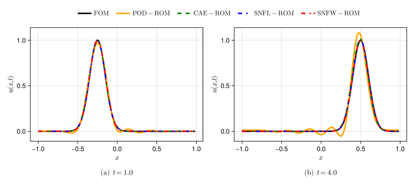
Figure 3: 1D scalar advection test case: comparison of different ROM predictions with the FOM solution. The predicted solutions for CAE-ROM, SNFW-ROM, and SNFL-ROM overlap and match the FOM solution, whereas those for POD-ROM suffer from large oscillations.

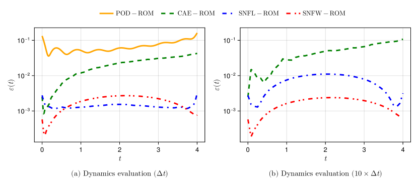
Figure 4: 1D scalar advection test case: error evolution of ROM predictions in time for dynamics evaluation with the (a) baseline $\Delta t$, and (b) 10 $\times$ $\Delta t$. The error for CAE-ROM grows with time for both cases, while the error for SNFW-ROM remains consistently low. The curve for POD-ROM is omitted from (b) due to large error values.

The first test case involves solving the 1D scalar advection equation,

$$\frac{\partial u}{\partial t}+c\frac{\partial u}{\partial x}=0,$$ (52)

which governs the transport of a scalar $u$. The advective velocity is selected to be $c=0.25$. A Gaussian signal,

$$u_{0}(x)=\exp\left\{\frac{-(x-\mu_{0})^{2}}{2\sigma_{0}^{2}}\right\},$$ (53)

with $\mu_{0}=-0.5$ and $\sigma_{0}=0.1$, is used to initialize the problem. As advection is the only transport mechanism for the scalar in this test case, it suffers from a slow decay of the Kolmogorov $n$-width, thereby motivating the need for nonlinear model reduction approaches.

Figure 5: 1D scalar advection test case: time-evolution of the ROM state vector $\tilde{u}(t)=\begin{bmatrix}\tilde{u}_{1}(t)&\tilde{u}_{2}(t)\end{bmatrix}^{T}$. The blue and red curves correspond to the first ($\tilde{u}_{1}$) and second $(\tilde{u}_{2})$ components respectively. For CAE-ROM, $\tilde{u}(t)$ from the dynamics evaluation deviates from the learned trajectory, whereas the curves from dynamics evaluations and the learned trajectory overlap for both SNFL-ROM and SNFW-ROM.

A comparison of ROM predictions with the FOM solution is shown in Figure 3 for $t=1$ and $t=4$. The figure indicates that the nonlinear ROMs give close predictions to FOM in both instances. On the other hand, POD-ROM leads to oscillations in the solution that become more prominent near the wave. A more detailed analysis of the differences between the ROM approaches requires assessing the temporal variation of the error, as defined in Eq. 51. Figure 4 presents the error evolution of ROMs from a dynamics evaluation with the baseline $\Delta t$, and a dynamics evaluation with a $10\times$ larger $\Delta t$. POD-ROM exhibits a large error at all times, indicating that a larger ROM representation is required to capture physics accurately. The curve for POD-ROM is omitted from Figure 4(b) due to large errors. In contrast, the nonlinear ROMs yield lower errors with a much smaller $N_{\text{ROM}}$. Despite a low initial value, the error in CAE-ROM grows steadily with time for both $\Delta t$, and reaches close to the POD-ROM error levels. The two SNF-ROM variants produce much lower errors for both $\Delta t$, though we observe a dramatic rise in error for SNFL-ROM with the larger time step size between $t=0.5$ and $t=3.5$. In contrast, SNFW-ROM produces consistently low errors for both $\Delta t$.

We analyze the trajectories of the ROM state vector for the nonlinear ROMs in Figure 5 to assess deviation between predictions of $\tilde{u}(t)$ learned during training (solid lines) and $\tilde{u}(t)$ obtained from dynamics evaluations (dotted lines correspond to a dynamics evaluation with the baseline $\Delta t$, and dashed lines correspond to a dynamics evaluation with a $10\times$ larger $\Delta t$). The first and second components of $\tilde{u}(t)=\begin{bmatrix}\tilde{u}_{1}(t)&\tilde{u}_{2}(t)\end{bmatrix}^{T}$ are represented by blue and red curves respectively. Figure 5 indicates that the three nonlinear ROMs learn ROM state trajectories that are smooth and continuous. SNFL-ROM and SNFW-ROM explicitly force this behavior by modeling $\tilde{u}$ as a simple and smooth function of $t$, which follows the expected trajectory accurately. For CAE-ROM, despite the initial proximity to the learned trajectory, ROM states from the dynamics evaluation with baseline $\Delta t$ deviate from the learned trajectory. This deviation corresponds to the growth in error with time for CAE-ROM presented in Figure 4 although further studies need to be conducted to ascertain causality. Furthermore, the ROM state trajectories for CAE-ROM obtained using a $10\times$ larger $\Delta t$ quickly deviate from the learned trajectory. This experiment illustrates that the dynamics evaluations of SNFL-ROM and SNFW-ROM are more accurate than those of other ROMs and support taking larger time steps.

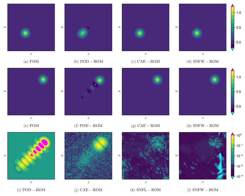
Figure 6: 2D scalar advection test case. Top row: prediction at $t=1$. Middle row: prediction at $t=4$. Bottom row: error in prediction $\epsilon(\boldsymbol{x},t)$ at $t=4$. The nonlinear ROMs match the FOM solution at both times, whereas POD-ROM produces large numerical oscillations. At $t=4$, SNFL-ROM and SNFW-ROM produce much smaller error values than POD-ROM and CAE-ROM. The predictions from SNFL-ROM at $t=1,\,4$, omitted due to space constraints, are indistinguishable from the FOM solution as indicated by the low error values in (k) and in Figure 7.

6.2 2D scalar advection test case

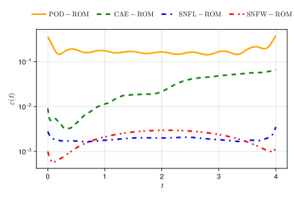
Figure 7: 2D scalar advection test case: temporal variation of error in ROM predictions. POD-ROM has the largest error at all time instances. The error in CAE-ROM grows with time, while SNFL-ROM and SNFW-ROM produce low errors that do not increase with time.

In this test case, we demonstrate the applicability of our model reduction approach for a 2D advection problem given by the equation

$$\frac{\partial u}{\partial t}+\boldsymbol{c}\cdot\gradient u=0,$$ (54)

where $\boldsymbol{c}=\begin{bmatrix}0.25&0.25\end{bmatrix}^{T}$ is the advection velocity. The solution is initialized with

$$u_{0}(\boldsymbol{x})=\exp\left\{\frac{-\norm{\boldsymbol{x}-\boldsymbol{\mu}_{0}}_{2}^{2}}{2\sigma_{0}^{2}}\right\},$$ (55)

where $\boldsymbol{\mu}_{0}=\begin{bmatrix}-0.5&-0.5\end{bmatrix}^{T}$ and $\sigma_{0}=0.1$.

The solution prediction at different time instances is shown in Figure 6. We observe oscillations in POD-ROM predictions even at an early time of $t=1$. These oscillations grow significantly and distort the solution by time $t=4$. The nonlinear ROMs, which include CAE-ROM, and SNFW-ROM, yield accurate results for both instances that match the FOM solution well. The final row of Figure 6 presents the distribution of $\epsilon(\boldsymbol{x},t)$ at the final time step for the four ROMs considered in this study. We notice that POD-ROM oscillations have grown larger in magnitude than the FOM solution. CAE-ROM has markedly lower errors in large parts of the domain. However, this error is roughly $10\%$ near the solution peak. SNFL-ROM has a much smaller overall error, whereas SNFW-ROM has the lowest error among all models with $\epsilon(\boldsymbol{x},t)<1\%$ everywhere in $\Omega$. A more quantitative comparison of accuracy can be observed by assessing the error metric defined in Figure 7.

The temporal variation of $\varepsilon(t)$ is shown in Figure 7. Consistently high errors are observed for POD-ROM compared to nonlinear ROMs. CAE-ROM exhibits comparatively lower error for the initial time $t<0.5$. However, this error grows in time to about $10\%$ of the solution magnitude. On the other hand, both SNFL-ROM and SNFW-ROM produce consistently low errors that do not grow in time, with SNFW-ROM exhibiting the lowest errors. With nearly constant errors, SNFL-ROM and SNFW-ROM are better suited for longer time dynamics predictions compared to POD-ROM and CAE-ROM. These results highlight the robustness of smooth neural fields in yielding consistently accurate representation for 2D advection-dominated problems, which have proven challenging for other ROM approaches as observed from the results.

6.3 1D viscous Burgers test case

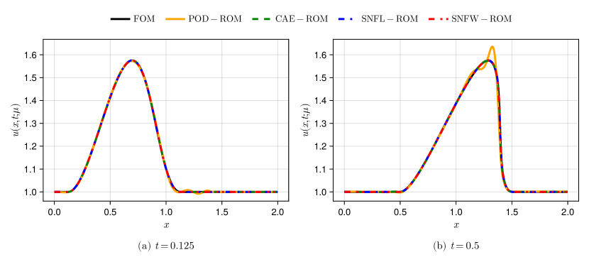
Figure 8: 1D viscous Burgers test case: comparison of ROM predictions with the FOM solution at $\mu=0.575$. The predicted solutions for CAE-ROM, SNFL-ROM, and SNFW-ROM agree well with the FOM solution, while POD-ROM produces spurious oscillations near the shock.

We consider 1D viscous Burgers equation,

$$\frac{\partial u}{\partial t}+u\frac{\partial u}{\partial x}=\nu\frac{\partial^{2}u}{\partial x^{2}},$$ (56)

where the viscosity $\nu=10^{-4}$ resulting in a Reynolds number of $10,000$. The PDE is initialized with a sinusoidal solution profile,

$$u_{0}(x;\mu)=\begin{cases}1+\frac{\mu}{2}\left(1+\sin\left(2\pi x-\frac{\pi}{2}\right)\right)&x\in[0,1]\\ 0&\text{otherwise}\end{cases},$$ (57)

parameterized by a scalar $\mu\in\mathbb{R}_{+}$. The solution to this equation involves the transport of a wavefront that eventually forms a shock. Accurate resolution of this shock typically requires a large number of linear modes from POD, and a key goal of nonlinear ROMs is to handle such physics with smaller reduced space representation. This test case is also used to demonstrate the applicability of proposed ROM approaches for parameter space exploration problems. In particular, FOM simulations with $\mu_{\text{train}}=\{0.5,0.55,0.6\}$ are used to train the ROM models. The ROMs are then evaluated for $\mu_{\text{test}}=\{0.525,0.575,0.625\}$. These tests enable the comparison of ROM approaches for both parameter space interpolation ($\mu\in\{0.525,0.575\}$) and extrapolation ($\mu=0.625$).

The comparison of different ROMs with FOM at two different time instances is shown in Figure 8 for $\mu=0.575$. All ROMs agree well with the FOM at $t=0.25$s, though POD-ROM exhibits small oscillations on the downstream end of the wave. These oscillations grow significantly and exhibit a large deviation from the FOM result near the shock at $t=0.5$. All nonlinear model reduction approaches exhibit high accuracy and adequately capture the shock.

A more detailed comparison of accuracy involves assessing the evolution of error in time for both training and validation datasets as shown in Figure 9. The three nonlinear ROMs perform well on the training case (Figure 9(a): $\mu=0.600$), whereas POD-ROM exhibits large errors. This was expected due to its inability to capture the shock in Figure 8. While all models experience growth in error with time, only SNFW maintains $<0.1\%$ error in $\varepsilon(t;\boldsymbol{\mu})$ for all time. For all models, the errors appear to be consistent between the training case and the interpolation case, indicating that their performance does not deteriorate significantly within the parameter space.

For the interpolation case (Figure 9(b): $\mu=0.575$), SNFW-ROM yields the lowest errors with time, whereas CAE-ROM and SNFL-ROM yield slightly larger errors. The errors on the extrapolation case (Figure 9(c): $\mu=0.625$) are markedly larger for all nonlinear ROMs, though POD-ROM still produces the greatest error values. The error in SNFL-ROM is consistent at $0.1\%$ until $t=0.4$, after which it increases to $1\%$. Similarly, the error in CAE-ROM remains consistent at a low value close to the end of the simulation, when it shoots up to $1\%$. Although SNFW-ROM experiences a rise in error close to $t=0.5$, the ROM maintains $\sim 0.1\%$ error at all times.

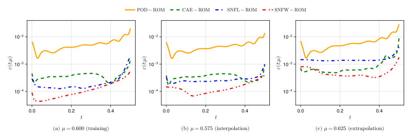
Figure 9: 1D viscous Burgers test case: variation of error in ROM prediction against time. All ROMs experience a rise in error with time on the extrapolation case ($\mu=0.625$). POD-ROM has the largest error. CAE-ROM and SNFL-ROM have similar error values, whereas SNFW-ROM performs the best for all cases.

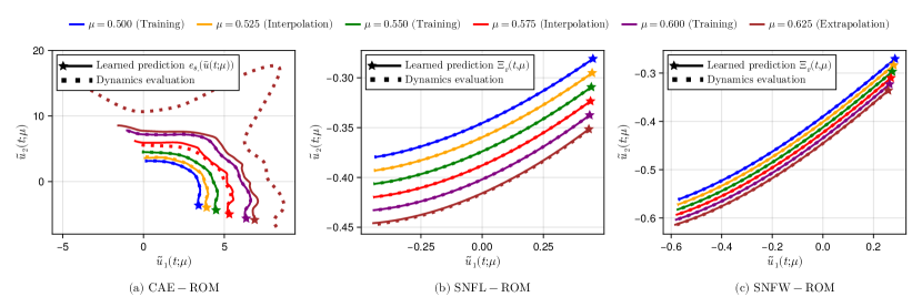
Figure 10: 1D viscous Burgers test case: distribution of ROM state vectors $\tilde{u}(t;{\mu})=\begin{bmatrix}\tilde{u}_{1}(t;{\mu})&\tilde{u}_{2}(t;{\mu})\end{bmatrix}^{T}$. The stars mark the beginning of the learned trajectories at $t=0$. In comparison to CAE-ROM, the SNFL-ROM and SNFW-ROM produce smooth, evenly-spaced learned trajectories that match with $\tilde{u}(t,\boldsymbol{\mu})$ from the dynamics evaluation. These results facilitate meaningful and robust interpolation and extrapolation in the parameter space.

To investigate the source of the error spikes near $t=0.5$, we examine the distribution of ROM state vectors $\tilde{u}$ for the nonlinear ROMs in Figure 10. The trajectories learned by CAE-ROM (Figure 10(a)) do not appear smooth and evenly spaced. For the interpolation case ($\mu=0.575$), the ROM state trajectories from the dynamics evaluation deviate from the learned trajectory, although this does not correspond to a marked rise in error.

In the extrapolation case ($\mu=0.625$), the ROM state trajectories from the dynamics evaluation of CAE-ROM (Figure 10(a)) deviate significantly from the learned trajectory for all time, although the error is low for $t<0.4$. This observation highlights that the deviation of ROM state trajectories from the dynamics evaluation away from the learned trajectory does not necessarily imply poor performance. As nonlinear ROMs parameterized by neural network functions may have multiple ROM state trajectories that yield low errors, the behavior of the dynamics evaluation away from the learned trajectory is unknown.

For the extrapolation case ($\mu=0.625$), the starting point for the dynamics evaluation for CAE-ROM (Figure 10(a)) has moved away from the encoder prediction by Gauss-Newton iteration in the manifold projection step (Section 5.1). We found that the Gauss-Newton step in manifold projection (Eq. 65) significantly improved the accuracy of CAE-ROM over initializing the dynamics evolution with encoder prediction at $t=0$. Although the ROM state trajectories from the dynamics evaluation remain away from the learned trajectory for all time, the error remains small till $t=0.4$. The large spike in error at $t>0.4$ illustrates that the dynamics evaluation is unreliable (away from the learned trajectory) and may produce inaccurate results.

We now investigate the ROM trajectories of SNFL-ROM and SNFW-ROM in Figure 10(b), Figure 10(c) respectively. The manifold constraint applied to SNFL-ROM and SNFW-ROM in Section 4.1 ensures that the trajectories are simple and evenly spaced. We note that for SNFL-ROM and SNFW-ROM, the ROM trajectories from the dynamics evaluation follow the learned trajectories for all $\mu$. In the extrapolation case ($\mu=0.625$), we observe a deviation between the learned trajectory and the dynamics evaluation for SNFL-ROM and SNFW-ROM near the end of the simulation. This deviation corresponds to the spike in error in both at $t=0.4$ in that case, although further investigation is needed to ascertain causality. This experiment highlights that SNF models are ideally suited for parametric space exploration problems and exhibit higher accuracy than other model reduction approaches considered in this article for both interpolation and extrapolation scenarios.

6.4 2D viscous Burgers test case

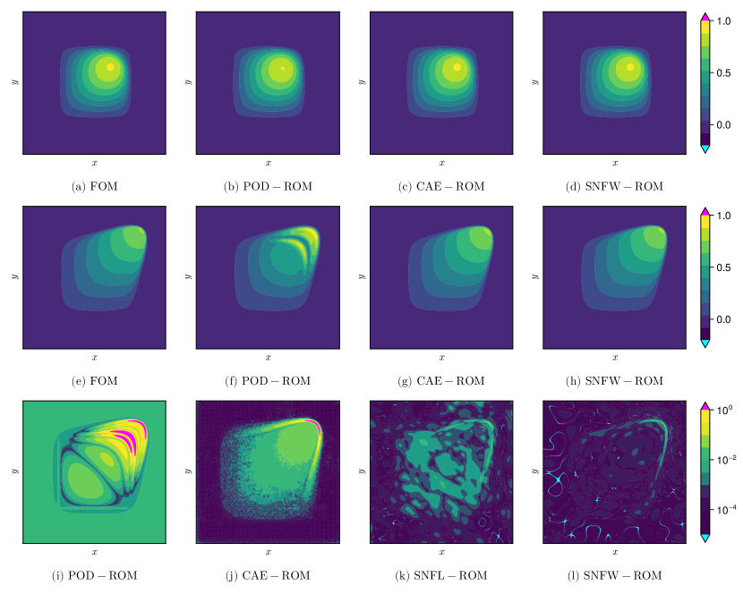
Figure 11: 2D viscous Burgers test case: Top row: prediction at $t=0.125$. Middle row: prediction at $t=0.5$. Bottom row: error $\epsilon(\boldsymbol{x},t)$ in prediction for ROM based at $t=0.5$. The nonlinear ROMs match the FOM solution at both times, while POD-ROM produces large oscillations. A quantitative error assessment indicates that SNFL-ROM and SNFW-ROM significantly outperform POD-ROM and CAE-ROM. The predictions from SNFL-ROM at $t=0.125,\,0.5$, omitted due to space constraints, are indistinguishable from the FOM solution as indicated by the low error values in (k) and in Figure 13.

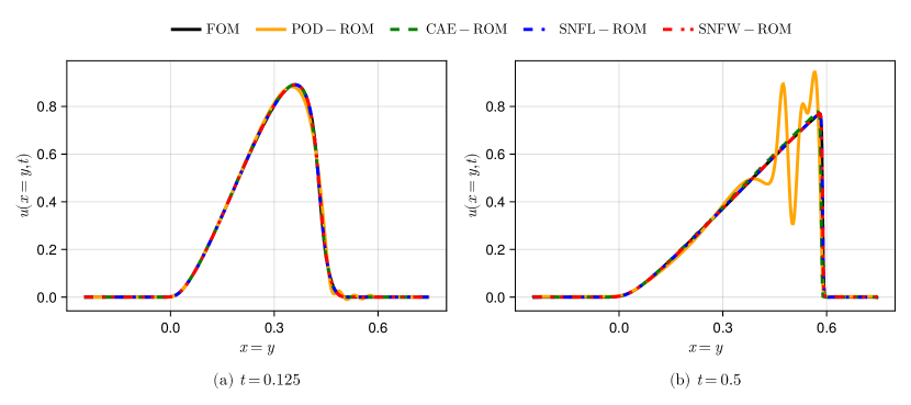
Figure 12: 2D viscous Burgers test case: comparison of ROM predictions with FOM solution along the slice $y=x$. CAE-ROM, SNFL-ROM and SNFW-ROM capture the steep shock at $t=0.5$, whereas POD-ROM suffers from large oscillations near the shock.

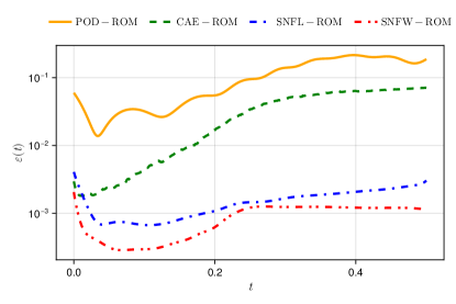
Figure 13: 2D viscous Burgers test case: temporal variation of error in ROM solutions. SNFL-ROM and SNFW-ROM produce low errors that do not grow with time, whereas errors for POD-ROM and CAE-ROM are high and grow with time.

To demonstrate the applicability of nonlinear model reduction for 2D problems with a shock front, we consider the 2D Burgers equation

$$\frac{\partial\boldsymbol{u}}{\partial t}+\boldsymbol{u}\cdot\nabla\boldsymbol{u}=\nu\Delta\boldsymbol{u},$$ (58)

where $\nu=10^{-3}$ is the viscosity resulting in a Reynolds number of $1,000$. Similar to the 1D Burgers test case, the solution propagates in time leading to a shock at $t=0.5$. The simulation is initialized to $\boldsymbol{u}_{0}(x,y)=\begin{bmatrix}u_{0}(x,y)&u_{0}(x,y)\end{bmatrix}^{T}$ where the scalar function $u_{0}$ is selected to be

$$u_{0}(x,y;\mu)=\begin{cases}\mu\sin\left(2\pi x\right)\sin\left(2\pi y\right)&x,y\in[0,0.5]\\ 0&\text{otherwise}\end{cases}.$$ (59)

The $x$ and $y$ components of $\boldsymbol{u}$ will be equal for all times as the problem is symmetric. Although the ROM models solve for both components, we restrict our analysis in Figure 11 and Figure 12 to the first component of the solution vector without loss of generality.

The solution at multiple time instances for different ROMs is shown in Figure 11. Similar to the 1D burgers test case, we observe that POD-ROM exhibits large oscillations and deviation from the FOM results at later times. All nonlinear model reduction approaches capture the shock well and exhibit much better accuracy than POD-ROM. A qualitative assessment of $\epsilon(\boldsymbol{x},t)$ indicates that CAE-ROM exhibits large errors near the shock front. SNFL-ROM and SNFW-ROM produce much smaller errors around the shock, as well as further away, with SNFW-ROM producing $\epsilon\leq 0.1\%$ errors everywhere at $t=0.5$.

This observation is more evident from results in Figure 12, which show ROM predictions along the diagonal slice $y=x$. We observe that POD-ROM exhibits a much higher error throughout the domain than nonlinear ROMs, which produce much more accurate results. The temporal evolution of error for different ROMs is shown in Figure 13. These results indicate that POD-ROM and CAE-ROM exhibit large errors that grow with time. Conversely, SNFL-ROM and SNFW-ROM experience a decrease in error at an early time, after which the error in SNFL-ROM rises steadily till the final time step, whereas the error in SNFW-ROM stabilizes to $\sim 0.1\%$. These results highlight the suitability of smooth neural fields, especially with weight regularization, to capture the physics of this 2D flow with a shock wave accurately and efficiently.

6.5 1D Kuromoto-Sivashinsky test case

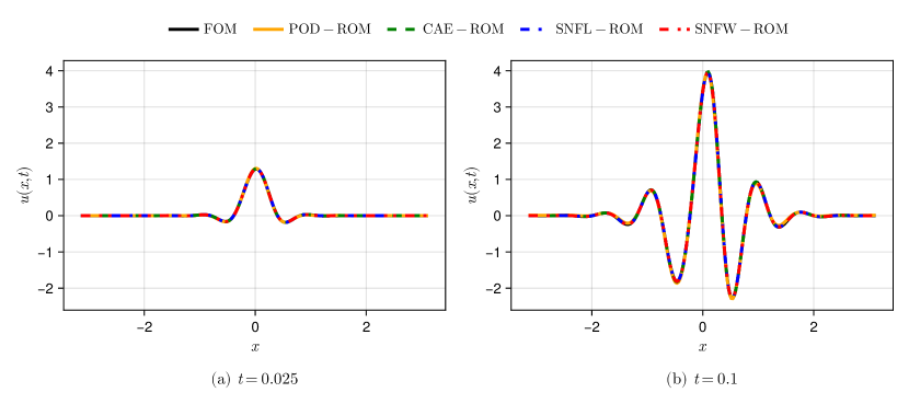
Figure 14: 1D Kuromoto-Sivashinsky test case: comparison of ROM predictions with the FOM solution. As this problem is highly diffusive ($\nu=0.01$), all linear and nonlinear ROMs agree with the FOM solution.

For the last test case, we select the Kuramoto-Sivashinsky (KS) equation to compare the performance of ROMs using nonlinear PDEs with higher-order derivatives. This PDE is given as,

$$\frac{\partial u}{\partial t}+u\frac{\partial u}{\partial x}+\frac{\partial^{2}u}{\partial x^{2}}+\nu\frac{\partial^{4}u}{\partial x^{4}}=0,$$ (60)

where $\nu=0.01$ is the viscosity. Higher-order derivatives in this problem make the dynamics difficult to predict. In particular, we note that the problem becomes high oscillatory results indicating unstable behavior for large number of POD modes. As such, we solve this problem with $N_{\text{ROM}}=2$ for POD-ROM. In comparison, nonlinear ROMs did not show a significant difference in performance between $N_{\text{ROM}}=1,\,2$. We present results here for $N_{\text{ROM}}=1$ for nonlinear ROMs. The PDE is initialized with

$$u_{0}(x)=\exp\left\{\frac{-x^{2}}{2\sigma_{0}^{2}}\right\},$$ (61)

where $\sigma_{0}=0.2$. As the solution of this equation is chaotic with a large sensitivity to the initial conditions, we only compare the ROMs at an initial short time window.

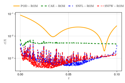
Figure 15: 1D Kuromoto-Sivashinsky test case: variation of error in ROM predictions against time. Despite large oscillations in error values, the error in nonlinear ROMs remains below $1\%$ at all times. SNFW-ROM produces low error values at all times. Note that the $y$-axis in this figure has $\log$ scale, which may distort the oscillations in the error curves for the nonlinear ROMs.

A comparison of solutions using different ROMs at two time instances is shown in Figure 14. The solution grows from a Gaussian initial condition to a complex signal with varying magnitudes. As the problem is highly diffusive, all ROMs appear to give similar results that are in good agreement with FOM. To compare these approaches more closely, we analyze the temporal evolution of error defined in Eq. 51. The temporal evolution of model error for different ROMs is shown in Figure 15. POD-ROMs exhibit the highest error for all instances of time that are tested. CAE-ROMs exhibit a lower error value that remains consistent over time. SNFL-ROMs exhibit a much smaller error in the initial time window, which grows considerably with time and reaches the same magnitude as CAE-ROM. SNFW-ROM, on the other hand, exhibits low error at all times of approximately $0.2\%$. This result follows the observation from other test cases that weighted decay regularization yields consistently more accurate results. We observe large oscillations in the error curves for SNFL-ROM and SNFW-ROM in Figure 15 whose origin is not fully understood. However, despite these oscillations, the errors are consistently below those for POD-ROM and CAE-ROM indicating superior performance of proposed SNF-ROMs.

7 Conclusions and discussion

SNF-ROM is a machine learning-based nonlinear model order reduction method that predicts dynamics by combining neural field spatial representations from point-cloud datasets with Galerkin projections. Compared to existing nonlinear ROMs, SNF-ROM presents several advantages in the online stage of dynamics prediction. SNF-ROM constrains the learned ROM manifold to be smooth and regular, thus allowing for robust online stage evaluations with large time steps. By supporting AD-based spatial differencing, SNF-ROM drastically simplifies the computation of online dynamics. Numerical experiments reveal that the dynamics evaluation of SNF-ROM is accurate and that the proposed smoothing methodology is robust, thus eliminating the need for hyperparameter tuning. While offering the key advantages mentioned above, SNF-ROM consistently outperforms other tested ROM approaches across various PDE problems.

SNF-ROM is not without limitations. For one, the offline training cost is significantly greater than that for a linear POD-ROM. This higher cost is a significant hurdle in working with nonlinear ROMs, as large training times bottleneck prototyping and experimentation processes. Future work may consider using modern neural architectures that support fast training [39]. Another possible research direction could be to use transformer-based meta-learning approaches to learn network weights [40] quickly. Many nonlinear ROMs are unable to handle complex and changing boundary conditions; future work could be directed towards alleviating this limitation. Future work may also consider lowering the cost of the online stage by integrating novel hyper-reduction schemes within SNF-ROM. Further performance gains may be achieved by writing customized GPU kernels for the online stage and employing highly efficient Taylor mode AD [41, 42] instead of forward mode AD. Nonlinear reduced order modeling is an emerging technology in its nascent stage. This work has identified and eliminated critical shortcomings in existing approaches. Substantial enhancements must be made for its maturation and practical application.

Appendix A CAE-ROM: Manifold projection

The CAE-ROM manifold projection function $h^{\prime}_{\text{CAE}}$ maps FOM state vectors $\overline{u}\in\mathbb{R}^{N_{\text{FOM}}}$ to corresponding ROM state vectors ${\tilde{u}}\in\mathbb{R}^{N_{\text{ROM}}}$ such that $h^{\prime}_{\text{CAE}}(\overline{u})$ reproduces $\overline{u}$ with $g^{\prime}_{\text{CAE}}$ to a reasonable accuracy. That is,

$$\overline{u}\approx g^{\prime}_{\text{CAE}}\circ h^{\prime}_{\text{CAE}}(\overline{u}).$$ (62)

Previous CAE-ROM implementations [11, 12] have employed the learned encoder for this task:

$$h^{\prime}_{\text{CAE}}:\overline{u}\to e_{\theta_{e}}(\overline{u}).$$ (63)

In our experiments, we found that the encoder prediction by itself may not be a local optimum solution to the nonlinear system

$$\operatorname*{argmin}_{{\tilde{u}}}\norm{\overline{u}-g^{\prime}_{\text{CAE}}({\tilde{u}})}^{2}_{2}.$$ (64)

As such, we solve this nonlinear least squares problem with Gauss-Newton iteration to implement $h^{\prime}_{\text{CAE}}$,

$$h^{\prime}_{\text{CAE}}(\overline{u})=\operatorname*{argmin}_{{\tilde{u}}}\norm{\overline{u}-g^{\prime}_{\text{CAE}}({\tilde{u}})}^{2}_{2},$$ (65)

where the initial guess is the encoder prediction $e_{\theta_{e}}(\overline{u})$. Our experiments indicate that using Gauss-Newton iteration to implement $h^{\prime}_{\text{CAE}}$ performed significantly better than simply using the encoder prediction as in Eq. 64.

Appendix B SNF-ROM: Manifold projection

We define the SNF-ROM manifold projection function $h_{\theta}$. Given a vector field $\boldsymbol{u}:\Omega\to\mathbb{R}^{m}$, $h_{\theta}$ seeks ROM state vector ${\tilde{u}}\in\mathbb{R}^{N_{\text{ROM}}}$ that can reconstruct $\boldsymbol{u}$ to a reasonable accuracy. That is,

$$\boldsymbol{u}(\boldsymbol{x})\approx g_{\theta}\left(\boldsymbol{x},h_{\theta}(\boldsymbol{u})\right),\,\forall\boldsymbol{x}\in\Omega.$$ (66)

Unlike discretization-dependent ROMs where the projection functions map between finite-dimensional fields, $h_{\theta}$ maps the continuous fields over $\Omega$ to $\mathbb{R}^{N_{\text{ROM}}}$. We close this problem by selecting a small subset of points $X_{\text{proj}}\subset\Omega$ where we attempt to satisfy Eq. 66

$$\boldsymbol{u}(\boldsymbol{x})\approx g_{\theta}\left(\boldsymbol{x},h_{\theta}(\boldsymbol{u})\right),\,\forall\boldsymbol{x}\in X_{\text{proj}}.$$ (67)

The choice of points in $X_{\text{proj}}$ is not restricted to $X_{\text{FOM}}$ and can be sampled anywhere in $\Omega$. Although only $N_{\text{ROM}}$ points are needed for solving Eq. 67, the system is typically over-determined [13] with $N_{\text{ROM}}<\absolutevalue{X_{\text{proj}}}<<N_{\text{FOM}}$ where $\absolutevalue{X_{\text{proj}}}$ is the number of points in $X_{\text{proj}}$.

If the intrinsic coordinates $(t,\boldsymbol{\mu})$ of $\boldsymbol{u}$ are known, then $\tilde{u}(t;\boldsymbol{\mu})$ can be predicted using the intrinsic ROM manifold as $\Xi_{\varrho}$. That is,

$$h_{\theta}:\boldsymbol{u}(t;\boldsymbol{\mu})\to\Xi_{\varrho}(t,\boldsymbol{\mu}).$$ (68)

However, our experiments in Section 6 indicate that $\Xi_{\varrho}(t,\boldsymbol{\mu})$ is typically not the local optimum of the system

$$\operatorname*{argmin}_{\tilde{u}}\sum_{\boldsymbol{x}\in X_{\text{proj}}}\norm{\boldsymbol{u}(\boldsymbol{x})-g_{\theta}(\boldsymbol{x},\tilde{u})}^{2}_{2}.$$ (69)

As such, we implement $h_{\theta}$ by solving Eq. 69 with Gauss-Newton iteration where the initial guess is given by $\Xi_{\varrho}(t,\boldsymbol{\mu})$. Our experiments indicate that using Gauss-Newton iteration for manifold projection leads to marginal improvements in accuracy over simply using $\Xi_{\varrho}(t,\boldsymbol{\mu})$.

Appendix C SNF-ROM: Architecture and training details

We discuss the implementation details in manifold construction of SNF-ROM. Given the tuple $\left(\boldsymbol{x},t,\boldsymbol{\mu}\right)$, we make a prediction for $\boldsymbol{u}(\boldsymbol{x},t;\boldsymbol{\mu})$ as follows. First, we obtain the ROM state vector corresponding to $t$, $\boldsymbol{\mu}$ on the intrinsic ROM manifold $\mathcal{\tilde{U}}$ as ${\tilde{u}}(t;\boldsymbol{\mu})=\Xi_{\varrho}(t,\boldsymbol{\mu})$. Then the query point $\boldsymbol{x}$ is concatenated with ${\tilde{u}}(t;\boldsymbol{\mu})$. The concatenated vector is then passed to the MLP, $g_{\theta}$. In the backward pass, the gradients are calculated with respect to $\theta$ and $\varrho$. See Figure 1 for reference.

In all experiments, the network $g_{\theta}$ has $7$ layers. The $5$ hidden layers have a fixed width $w$, whereas the sizes of the input and output layers are $d+N_{\text{ROM}}$ and $m$ respectively. A sine activation function, i.e. $\sigma(x)=\sin(x)$, is chosen for the ability of sinusoidal networks to fit high-frequency functions [16]. The final layer of the network does not use a bias vector. The network $\Xi_{\varrho}$ is chosen to be a shallow MLP with width $8$. The network is purposely chosen to be small so that simple ROM representations are learned. The tanh activation function is chosen to ensure that ROM state vectors are continuous functions of $t$ and $\boldsymbol{\mu}$. Furthermore, we apply $L^{2}$ regularization with $\gamma=10^{-3}$ on the parameters $\varrho$ to ensure that a smooth mapping is learned.

In $g_{\theta}$, the weight matrices have been initialized per the SIREN initialization scheme described in [16] to ensure a normal distribution of output values following a sine activation. This involves scaling the weight matrices in the network layers by constant $\omega$ during initialization. For the first layer, $\omega$ is set to $10$ to represent a wide range of frequencies [16], and $\omega=1$ for the following layers. The choice of $\omega$ directly affects the range of frequencies the model is able to represent, where low values encourage smoother functions, and larger values encourage high-frequency and finely-detailed functions [43]. The final layer is initialized with Xavier initialization [44]. The initial bias vectors are sampled from a uniform random distribution to create a phase shift among the sinusoidals in each layer. For the network $\Xi_{\varrho}$, the weight matrices are initialized according to the Xavier initialization [44] scheme, and the biases are initialized to zero values.

We normalize the data set so that the spatial coordinates, the field values, and the times have zero mean and unit variance. Our training pipeline disaggregates simulation snapshots into tuples $(\boldsymbol{x},t,\boldsymbol{\mu},\boldsymbol{u}(\boldsymbol{x},\cdot))$ and stochastically composes the dataset $\mathcal{D}$ into $100$ equally-sized mini-batches. For SNFL-ROM, we use the Adam optimizer [45] for learning $\theta$, and $\varrho$. For SNFW-ROM, we use the AdamW optimizer [46] is employed as described in Section 4.2.2. While we formulate W regularization as an additional loss term, it can be easily implemented by modifying the weight-decay approach in an AdamW optimizer. Rather than computing the sensitivity of $L_{\text{Weight}}$ in Eq. 39 with respect to $\theta$ via backpropagation, the expressions can be written in closed form as

$$\nabla_{W^{ij}_{l}}L_{\text{Weight}}=\gamma W^{ij}_{l},\hskip 10.00002pt\nabla_{\theta_{i}}L_{\text{Weight}}=0\hskip 10.00002pt\text{for all other }\theta_{i}.$$ (70)

The sensitivity $\nabla_{\theta}L_{\text{W}}$ is computed per Eq. 39 and subtracted from $\theta$ at every optimization step [46].

We adopt the learning rate decay strategy outlined in [13]. We train for $200$ epochs at each learning rate in the schedule,

$$100\cdot\eta\to 10\cdot\eta\to 5\cdot\eta\to 1\cdot\eta\to 0.5\cdot\eta\to 0.2\cdot\eta\to 0.1\cdot\eta,$$ (71)

with a base learning rate of $\eta=10^{-4}$. Additionally, we run a learning rate warmup cycle for $10$ epochs at $\eta=0.01$. Early stopping is imposed if the loss value does not decrease for $20\%$ of consecutive epochs at any learning rate.

References

- [1] Thomas JR Hughes, Assad A Oberai, and Luca Mazzei. Large eddy simulation of turbulent channel flows by the variational multiscale method. Physics of Fluids, 13(6):1784–1799, 2001.
- [2] Haecheon Choi and Parviz Moin. Grid-point requirements for large eddy simulation: Chapman’s estimates revisited. Physics of Fluids, 24(1):011702, 2012.
- [3] Xuan Liang, Angran Li, Anthony D Rollett, and Yongjie Jessica Zhang. An isogeometric analysis-based topology optimization framework for 2D cross-flow heat exchangers with manufacturability constraints. Engineering with Computers, 38(6):4829–4852, 2022.
- [4] Shady E. Ahmed, Suraj Pawar, Omer San, Adil Rasheed, Traian Iliescu, and Bernd R. Noack. On closures for reduced order models - A spectrum of first-principle to machine-learned avenues. Physics of Fluids, 33(9):091301, 2021.
- [5] Nadine Aubry, Philip Holmes, John L. Lumley, and Emily Stone. The dynamics of coherent structures in the wall region of a turbulent boundary layer. Journal of Fluid Mechanics, 192:115–173, 1988.
- [6] David J. Lucia, Philip S. Beran, and Walter A. Silva. Reduced-order modeling: New approaches for computational physics. Progress in Aerospace Sciences, 40(1):51–117, 2004.
- [7] Constantin Greif and Karsten Urban. Decay of the Kolmogorov N-width for wave problems. Applied Mathematics Letters, 96:216–222, 2019.
- [8] Aviral Prakash and Yongjie Jessica Zhang. Projection-based reduced order modeling and data-driven artificial viscosity closures for incompressible fluid flows. Computer Methods in Applied Mechanics and Engineering, 425:116930, 2024.
- [9] B. Peherstorfer and K. E. Willcox. Data-driven operator inference for nonintrusive projection-based model reduction. Computer Methods in Applied Mechanics and Engineering, 306:196–215, 2016.
- [10] Aviral Prakash and Yongjie Jessica Zhang. Data-driven identification of stable differential operators using constrained regression, 2024. arXiv:2405.00198.
- [11] Kookjin Lee and Kevin Carlberg. Model reduction of dynamical systems on nonlinear manifolds using deep convolutional autoencoders. Journal of Computational Physics, 404:108973, 2020.
- [12] Youngkyu Kim, Youngsoo Choi, David Widemann, and Tarek Zohdi. A fast and accurate physics-informed neural network reduced order model with shallow masked autoencoder. Journal of Computational Physics, 451:110841, 2022.
- [13] Peter Yichen Chen, Jinxu Xiang, Dong Heon Cho, Yue Chang, G A Pershing, Henrique Teles Maia, Maurizio M Chiaramonte, Kevin Thomas Carlberg, and Eitan Grinspun. CROM: Continuous reduced-order modeling of PDEs using implicit neural representations. In The Eleventh International Conference on Learning Representations, 2023.
- [14] Ludovica Cicci, Stefania Fresca, and Andrea Manzoni. Deep-HyROMnet: A deep learning-based operator approximation for hyper-reduction of nonlinear parametrized PDEs. Journal of Scientific Computing, 93(2):57, 2022.
- [15] Yue Chang, Peter Yichen Chen, Zhecheng Wang, Maurizio M. Chiaramonte, Kevin Carlberg, and Eitan Grinspun. LiCROM: Linear-subspace continuous reduced order modeling with neural fields. In SIGGRAPH Asia, pages 1–12, 2023.
- [16] Vincent Sitzmann, Julien Martel, Alexander Bergman, David Lindell, and Gordon Wetzstein. Implicit neural representations with periodic activation functions. In Advances in Neural Information Processing Systems, volume 33, pages 7462–7473, 2020.
- [17] Jessica T. Lauzon, Siu Wun Cheung, Yeonjong Shin, Youngsoo Choi, Dylan Matthew Copeland, and Kevin Huynh. S-OPT: A points selection algorithm for hyper-reduction in reduced order models, 2022. arXiv:2203.16494.
- [18] Zhong Yi Wan, Leonardo Zepeda-Nunez, Anudhyan Boral, and Fei Sha. Evolve smoothly, fit consistently: Learning smooth latent dynamics for advection-dominated systems. In The Eleventh International Conference on Learning Representations, 2023.
- [19] Hsueh-Ti Derek Liu, Francis Williams, Alec Jacobson, Sanja Fidler, and Or Litany. Learning smooth neural functions via Lipschitz regularization. In ACM SIGGRAPH, pages 1–13, 2022.
- [20] Stefania Fresca, Luca Dedé, and Andrea Manzoni. A comprehensive deep learning-based approach to reduced order modeling of nonlinear time-dependent parametrized PDEs. Journal of Scientific Computing, 87:1–36, 2021.
- [21] Nikolaj T. Mücke, Sander M. Bohté, and Cornelis W. Oosterlee. Reduced order modeling for parameterized time-dependent PDEs using spatially and memory aware deep learning. Journal of Computational Science, 53:101408, 2021.
- [22] Igor A. Baratta, Joseph P. Dean, Jørgen S. Dokken, Michal Habera, Jack S. Hale, Chris N. Richardson, Marie E. Rognes, Matthew W. Scroggs, Nathan Sime, and Garth N. Wells. DOLFINx: The next generation FEniCS problem solving environment, https://doi.org/10.5281/zenodo.10447666, 2023.
- [23] J. R. Dormand and P. J. Prince. Runge-Kutta triples. Computers & Mathematics with Applications, 12(9, Part A):1007–1017, 1986.
- [24] C. F. Curtiss and J. O. Hirschfelder. Integration of stiff equations. Proceedings of the National Academy of Sciences of the United States of America, 38(3):235–243, 1952.
- [25] Alejandro N. Diaz, Youngsoo Choi, and Matthias Heinkenschloss. A fast and accurate domain decomposition nonlinear manifold reduced order model. Computer Methods in Applied Mechanics and Engineering, 425:116943, 2024.
- [26] Jeong Joon Park, Peter Florence, Julian Straub, Richard Newcombe, and Steven Lovegrove. DeepSDF: Learning continuous signed distance functions for shape representation. In IEEE/CVF Conference on Computer Vision and Pattern Recognition, 2019.
- [27] Jaehoon Cha and Jeyan Thiyagalingam. Disentangling autoencoders (DAE), 2022. arXiv:2202.09926.
- [28] Sifan Wang, Bowen Li, Yuhan Chen, and Paris Perdikaris. PirateNets: Physics-informed deep learning with residual adaptive networks, 2024. arXiv:2402.00326.
- [29] Aditya Chetan, Guandao Yang, Zichen Wang, Steve Marschner, and Bharath Hariharan. Accurate differential operators for hybrid neural fields, 2023. arXiv:2312.05984.
- [30] Jules Berman and Benjamin Peherstorfer. CoLoRA: Continuous low-rank adaptation for reduced implicit neural modeling of parameterized partial differential equations, 2024. arXiv:2402.14646.
- [31] Kevin Carlberg, Matthew Barone, and Harbir Antil. Galerkin v. least-squares Petrov-Galerkin projection in nonlinear model reduction. Journal of Computational Physics, 330:693–734, 2017.
- [32] Vedant Puri. FourierSpaces.jl: Fourier spectral PDE solvers in Julia. https://github.com/CalculustJL/FourierSpaces.jl, 2022.
- [33] Christopher Rackauckas and Qing Nie. DifferentialEquations.jl – A performant and feature-rich ecosystem for solving differential equations in Julia. Journal of Open Research Software, 5(1), 2017.
- [34] Jeff Bezanson, Stefan Karpinski, Viral B. Shah, and Alan Edelman. Julia: A fast dynamic language for technical computing, 2012. arXiv:1209.5145.
- [35] Avik Pal. On Efficient Training & Inference of Neural Differential Equations. Thesis, Massachusetts Institute of Technology, 2023.
- [36] Tim Besard, Christophe Foket, and Bjorn De Sutter. Effective extensible programming: Unleashing Julia on GPUs. IEEE Transactions on Parallel and Distributed Systems, 30(4):827–841, 2019.
- [37] Michael Innes. Don’t unroll adjoint: Differentiating SSA-Form programs, 2019. arXiv:1810.07951.
- [38] Jarrett Revels, Miles Lubin, and Theodore Papamarkou. Forward-mode automatic differentiation in Julia, 2016. arXiv:1607.07892.
- [39] Thomas Müller, Alex Evans, Christoph Schied, and Alexander Keller. Instant neural graphics primitives with a multiresolution hash encoding. ACM Transactions on Graphics, 41(4):102:1–102:15, 2022.
- [40] Yinbo Chen and Xiaolong Wang. Transformers as meta-learners for implicit neural representations. In European Conference on Computer Vision, pages 170–187, 2022.
- [41] Songchen Tan. Taylordiff.jl: Fast higher-order automatic differentiation in Julia. https://github.com/JuliaDiff/TaylorDiff.jl, 2022.
- [42] James Bradbury, Roy Frostig, Peter Hawkins, Matthew James Johnson, Chris Leary, Dougal Maclaurin, George Necula, Adam Paszke, Jake VanderPlas, Skye Wanderman-Milne, and Qiao Zhang. JAX: Composable transformations of Python+NumPy programs, http://github.com/google/jax, 2018.
- [43] David Wiesner, Julian Suk, Sven Dummer, David Svoboda, and Jelmer M. Wolterink. Implicit neural representations for generative modeling of living cell shapes. In Medical Image Computing and Computer Assisted Intervention, pages 58–67, 2022.
- [44] Siddharth Krishna Kumar. On weight initialization in deep neural networks, 2017. arXiv:1704.08863.
- [45] Diederik P. Kingma and Jimmy Ba. Adam: A method for stochastic optimization, 2017. arXiv:1412.6980.
- [46] Ilya Loshchilov and Frank Hutter. Decoupled weight decay regularization. In International Conference on Learning Representations, 2019.