A Seifert algorithm for integral homology spheres.

Abstract.

From classical knot theory we know that every knot in $S^{3}$ is the boundary of an oriented, embedded surface. A standard demonstration of this fact achieved by elementary technique comes from taking a regular projection of any knot and employing Seifert’s constructive algorithm. In this note we give a natural generalization of Seifert’s algorithm to any closed integral homology 3-sphere. The starting point of our algorithm is presenting the handle structure of a Heegaard splitting of a given integral homology sphere as a planar diagram on the boundary of a $3$-ball. (For a well known example of such a planar presentation, see the Poincaré homology sphere planar presentation in Knots and Links by D. Rolfsen [4].) An oriented link can then be represented by the regular projection of an oriented $k$-strand tangle. From there we give a natural way to find a “Seifert circle” and associated half-twisted bands.

1. Introduction

In Herbert Seifert’s seminal paper, “Über das Geschlecht von Knoten” [5], a simple constructive algorithm is described that starts with a regular projection of a given oriented knot (or link) on an $S^{2}$ in $S^{3}$ and yields an oriented surface having the given knot (or link) as its boundary—notably the surface has a visible presentation that “overlays” the knot projection. From there Seifert gives us a tour de force, defining a matrix that describes the homology relations of his Seifert surface, then utilizes this Seifert matrix to produce an efficient method of computing the Alexander polynomial. So constructed, he then demonstrates that half the degree of the Alexander polynomial is a lower bound for the genus of the Seifert surface. Finally, he investigates the structure of polynomials that can be Alexander polynomials, even producing examples of non-trivial knots that have trivial Alexander polynomial.

The goal of this manuscript is to give a natural generalization of Seifert’s constructive algorithm to any closed integral homology $3$-sphere. To see the naturality of this generalization it is helpful to be more descriptive of Seifert’s elegant algorithm.

Seifert’s algorithm starts with a planar presentation of a genus-$0$ Heegaard diagram of $S^{3}$. That is, a $2$-sphere that gives a handle decomposition—one $3$-dimensional $0$-handle and one $3$-dimensional $3$-handle. The oriented knot in question is projected onto this $2$-sphere by a regular projection. Utilizing the orientation of the knot, the crossings of the projection are resolved and the resultant oriented Seifert circles bound a collection of disjoint discs in the $0$-handle of $S^{3}$. Thus, we have $2$-dimensional $0$-handles which are the start of a spanning surface positioned in the $0$-handle of our $3$-manifold’s handle decomposition. We recover the resolved crossing of the knot projection by attaching to this collection of disjoint discs half-twisted bands at each crossing. The resulting spanning surface should then be thought of as being in “pseudo-normal position”. That is, although the surface’s $0$-handles are well positioned with respect to the handle decomposition of $S^{3}$, this decomposition lacks $3$-dimensional $1$-handles in which the $2$-dimensional $1$-handles of Seifert’s construction—the half-twisted bands—might be positioned. Instead, these half-twisted bands are positioned arbitrarily close to the shared boundary sphere of the $0$-handle and $3$-handle in the handle decomposition of $S^{3}$.

Seifert’s algorithm can be thought of as a demonstration that $S^{3}$ is a homology $3$-sphere, having trivial first integral homology. Our constructive algorithm will start with a given oriented link in any integral homology sphere, $M$. The construction is based upon representing $M$ via a Heegaard splitting or, equivalently, a handle decomposition having exactly one $0$-handle. An oriented knot, $K\subset M$, is then in normal position in the $0$- and $1$-handles of the decomposition. (Please see §2 for formal definition of handle decomposition and normal position.) With respect to this normal position, if $K$ goes through the $1$-handles $n$ times, then $K$ can be represented by a regular projection of an $n$-tangle on the boundary of the unique $0$-handle. If we are considering oriented links then we must allow the $n$-tangle to possibly have $S^{1}$ components that are totally contained in the unique $0$-handle.

The algorithm will produce a spanning surface which is in pseudo-normal position with respect to the handle decomposition of $M$. That is, the spanning surface will also have a handle decomposition where its $0$- and $2$-handles are properly embedded in the $0$- and $2$-handles of $M$, respectively. Additionally, its $1$-handles come in two flavors: those properly embedded in the $1$-handles of $M$ and those that are half-twisted bands at crossings of the $n$-tangle projection in an arbitrarily close neighborhood of the boundary of the $0$-handle of $M$.

Our paper is organized as follows. In §2 we review the needed definitions of handle decompositions for $2$-manifolds with boundary and closed oriented $3$-manifolds.

In §2.6.1 we describe the spanning surface algorithm. Since there is a needed homological calculation for determining how many times a spanning surface intersects a given $2$-handle of $,M$, we provide the reader with an example of knots in the Poincaré homology sphere in §3.

The example discussed in §3 is based upon a geometric calculation—taking $+1$ Dehn surgery on the trefoil and producing a Heegaard diagram—lifted from D. Rolfsen’s seminal book, Knots and Links [4]. We offer a method for generalizing this calculation for arbitrary framed links in §4.

We end the paper with an open question in section §5.

2. Definitions

First, we specify some of our notation. The cardinality of a set or collection, $X$, will be denoted by $|X|$. The interior of a topological set, $X$, will be denoted by, $int(X)$. For an oriented, $n$-dimensional manifold $M^{n}$, $-M^{n}$ will denote the same manifold with orientation reversed. An orientation preserving and orientation reversing map will be denoted by $\phi^{+}$ and $\phi^{-}$, respectively. $B^{k}$ will be notation for a closed ball of dimension $k$ and $c(B^{k})$ will denote the center point of the $k$-ball. The sign function, which we will denote with $\sigma(x)$ is defined as follows: $\sigma(x)=\begin{cases}+&\text{ if }|x|=x\\ -&\text{ otherwise}\end{cases}$

To facilitate a straightforward expository, we begin with the needed definitions specialized to dimensions $0$, $1$, $2$ and $3$.

2.1. Handle Structure and Orientation

An $n$-dimensional $k$-handle is a $n$-ball having product structure, $B^{k}\times B^{n-k}$. The core of a $k$-handle is $C^{k}:=B^{k}\times c(B^{n-k})$, and the co-core is $C^{k\ast}:=c(B^{k})\times B^{n-k}$.

There are then two natural projection maps, $\pi:B^{k}\times B^{n-k}\rightarrow C^{k}$, and $\pi^{\ast}:B^{k}\times B^{n-k}\rightarrow C^{k\ast}$.

For $n=2,3$ we begin with an oriented 0-handle. We then choose an orientation for the core, $C^{1}$, of the 1-handle. This induces an orientation on the co-core, $C^{1*}$, of the 1-handle (such that the algebraic intersection between $C^{1}$ and $C^{1*}$ is positive). Now, with $C^{1}$ oriented, we note that the boundary of $C^{1}$ consists of two points which we can appropriately denote by $c^{+}$ and $c^{-}$. Additionally, we will denote by $\mathbb{B}^{\pm}:=c^{\pm}\times B^{n-k}$ the attaching region of the 1-handle. For the 2-handle, choose the orientation on it so that it is coherent with the orientation of the 0-handle. Note that there is a choice to be made on the orientation of the 2-handle. In particular, after choosing an orientation on the boundary of the core, $\partial(C^{2}$), of a 2-handle, an orientation is induced on the co-core, $C^{2*}$ of the 2-handle.

2.2. Handle decomposition

Definition 1 (Compact surface with boundary).

For a compact surface with boundary, $\Sigma^{2}$, a handle decomposition of $\Sigma^{2}$ consists of:

• A finite collection of 0-handles $\{B^{0}\times B^{2}\}_{p}$ such that $\mathbf{H}_{0}^{2}:=\bigsqcup_{p}(B^{0}\times B^{2})\subset\Sigma^{2}$, where $\partial\mathbf{H}_{0}^{2}=\bigsqcup_{p}\partial(B^{0}\times B^{2})(\cong\bigsqcup_{p}S^{1})$.

• A finite collection of 1-handles $\{B^{1}\times B^{1}\}_{q}$ such that $\mathbf{H}_{1}^{2}:=\bigsqcup_{q}(B^{1}\times B^{1})\subset\Sigma^{2}$, and non-intersecting attaching maps $\{\phi^{\pm}\}_{q}$, where $\phi^{\pm}:\mathbb{B}^{\pm}\rightarrow\partial\mathbf{H}_{0}^{2}$.

• A finite collection of 2-handles $\{B^{2}\times B^{0}\}_{r}$ such that $\mathbf{H}_{2}^{2}:=\bigsqcup_{r}(B^{2}\times B^{0})\subset\Sigma^{2}$, and non-intersecting attaching maps $\{\psi^{\pm}\}_{r}$, where $\psi^{\pm}:\partial B^{2}\times B^{0}\rightarrow\partial\left(\mathbf{H}_{0}^{2}\bigsqcup\mathbf{H}_{1}^{2}/\{\phi^{\pm}\}_{q}\right)$

Then,

$$\frac{\mathbf{H}^{2}_{0}\sqcup\mathbf{H}^{2}_{1}\sqcup\mathbf{H}^{2}_{2}}{\{\phi^{\pm}\}_{p}\cup\{\psi^{\pm}\}_{q}}\cong\Sigma^{2}.$$

The reader should recall that from a handle decomposition we have the Euler Characteristic,

$$\chi(\Sigma^{2})=\sum_{0\leq s\leq 2}(-1)^{s}|\mathbf{H}^{2}_{s}|.$$

As with the classical Seifert algorithm, we will be concerned only with oriented surfaces. For our spanning surface construction we require the following specialized definition of a $3$-manifold handle decomposition.

Definition 2 (Closed oriented $3$-manifolds).

For a closed orientable $3$-manifold, $M^{3}$, a handle decomposition of $M^{3}$ consists of:

• A unique 0-handle $\{B^{0}\times B^{3}\}=\mathbf{H}_{0}^{3}\subset M^{3}.$

• A finite collection of 1-handles $\{B^{1}\times B^{2}\}_{g}$ such that $\mathbf{H}_{1}^{3}:=\bigsqcup_{g}(B^{1}\times B^{2})\subset M^{3}$, and non-intersecting attaching maps $\{\varphi^{\pm}\}_{g}$ where $\varphi^{\pm}:\mathbb{B}^{\pm}\rightarrow\partial\mathbf{H}_{0}^{3}$.

• A finite collection of 2-handles $\{B^{2}\times B^{1}\}_{g}$ such that $\mathbf{H}_{2}^{3}:=\bigsqcup_{g}(B^{2}\times B^{1})\subset M^{3}$ and non-intersecting attaching maps $\{\varrho^{\pm}\}_{g}$ where $\varrho^{\pm}:\partial B^{2}\times B^{1}\rightarrow\partial\left(\mathbf{H}_{0}^{3}\bigsqcup\mathbf{H}_{1}^{3}/\{\varphi^{\pm}\}_{g}\right)$.

• A unique 3-handle $\{B^{3}\times B^{0}\}=\mathbf{H}_{3}^{3}\subset M^{3}$ with, up to isotopy, a unique attaching map $\varsigma:\partial\mathbf{H}_{3}^{3}\rightarrow\left(\mathbf{H}_{0}^{3}\bigsqcup\mathbf{H}_{1}^{3}\bigsqcup\mathbf{H}_{2}^{3}/\{\varphi^{\pm}\}_{g},\{\varrho^{\pm}\}_{g}\right)$

Then

(2.1) $$\frac{\mathbf{H}^{3}_{0}\sqcup\mathbf{H}^{3}_{1}\sqcup\mathbf{H}^{3}_{2}\sqcup\mathbf{H}^{3}_{3}}{\{\varphi^{\pm}\}_{g},\{\varrho^{\pm}\}_{g},\{\varsigma\}}\cong M^{3}$$

For later convenience, we assume the readily achievable technical condition ($\star$): for each pair of points, $(x,y)$, where $x$ is a point in the core of a handle in $\mathbf{H}^{3}_{1}$ and $y$ is a point in the co-core of a handle in $\mathbf{H}^{3}_{2}$, $\{x\}\times\partial B^{2}_{u}$ and $\partial B^{2}_{v}\times\{y\}$ intersect transversely, $1\leq u,v\leq g$.

2.3. The Heegaard Graph

From Definition 2 we can define, ${\mathscr{H}}\subset\partial\mathbf{H}^{3}_{0}$, a natural planar “fat graph” that captures all the information of a $3$-manifold’s handle decomposition.

Definition 3 (Heegaard Graph).

Given a Heegaard diagram $(F^{2},\alpha,\beta)$ of a genus $g$ Heegaard splitting of a 3-manifold, the corresponding Heegaard graph, ${\mathscr{H}}$, consists of a collection of (fat) vertices $\{V_{i}^{\pm}\}_{g}$ and edges $\{e_{j,l}\}$, for $1\leq i,j\leq g$, $1\leq l<\infty$, called ${\mathscr{H}}$-vertices and ${\mathscr{H}}$-edges, respectively. The $\{V_{i}^{\pm}\}_{g}$ represent the $g$ characteristic curves in $\alpha$, and the $\{e_{j,l}\}$ are such that $\{\bigcup_{l}e_{j,l}:1\leq j\leq g\}$ represent the $g$ characteristic curves in $\beta$. For each $i$, $V_{i}^{\pm}\bigcap e_{j,l}\not=\emptyset$ for at least one $l$. In particular, each nonempty intersection $V_{i}^{\pm}\bigcap e_{j,l}$ is a numbered point on $\partial V_{i}^{\pm}$. For each $i$, $V_{i}^{+}\xleftrightarrow{r}V_{i}^{-}$, where $r$ is a reflection.

${\mathscr{H}}$ has an orientation inherited from its Heegaard splitting. Also, ${\mathscr{H}}\subset S^{2}=\partial(B^{0}\times B^{3})$. We will denote by ${\mathcal{H}}_{0}$, the unique 0-handle of the Heegaard splitting on which we will be working on. That is, ${\mathscr{H}}\subset\partial{\mathcal{H}}_{0}$. From (2.1) above, it can be seen that the fat vertices, $\{V^{\pm}_{i}\}$, and edges, $\{e_{j,l}\}$, of a Heegaard graph are precisely the $\varphi(\mathbb{B}^{\pm}_{i})$ and $\varrho(\partial(B^{2}\times c(B^{1})))$, respectively.

2.4. Submanifolds in normal position

For the definitions in this section we assume that $\Sigma^{2}$ is a submanifold in $M^{3}$. Morover, we assume that both $\Sigma^{2}$ and $M^{3}$ have handle decompositions.

Definition 4 (Links in normal position).

Let $M^{3}$ be a closed oriented $3$-manifold with a handle decomposition and $L\subset M^{3}$ be a link. Then $L$ is in weak normal position with respect to the handle decomposition of $M^{3}$ if the following two conditions hold:

• $L$ is contained in the union of ${\mathcal{H}}_{0}$ and $\mathbf{H}_{1}^{3}$.

• (intersection with $\mathbf{H}_{1}^{3}$) For each $1$-handle, $B^{1}\times B^{2}$ of $\mathbf{H}_{1}^{3}$, with co-core $C^{1\ast}$, we require that $L\cap C^{1\ast}$ be a discrete set of points so that we have $L\cap[B^{1}\times B^{2}]=B^{1}\times[L\cap int(C^{1\ast})]$.

The link is in normal position with respect to the handle decomposition if it also satisfies the following:

• (intersection with ${\mathcal{H}}_{0}$) We require that $L\cap{\mathcal{H}}_{0}=L\cap\partial{\mathcal{H}}_{0}$– a collection of pairwise disjoint arcs and circles such that

  • Each arc has one endpoint contained in the interior of $\varphi(\mathbb{B}^{\pm}_{i})$ and the other contained in the interior of $\varphi(\mathbb{B}^{\pm}_{j})$, and its intersection with $\varphi(\mathbb{B}^{\pm}_{k})$ is empty for $k\not=i,j.$

  • Each circle component of $L\cap\partial{\mathcal{H}}_{0}$ is away from the $\varphi(\mathbb{B}_{i}^{\pm})$ (fat vertices) of ${\mathscr{H}}$.

We observe that every link is isotopic to one in weak normal position but not all links contained in $M^{3}$ are isotopic to a link in normal position since an isotopy that pushes a link so as to be contained in $\partial{\mathcal{H}}_{0}$ may result in double points (crossings)—the collection of arcs and circles are no longer simple or pairwise disjoint. With this in mind, we say a link is in pseudo-normal position if it satisfies condition–2.) except in a neighborhood of finitely many points in $\partial{\mathcal{H}}_{0}$ where a crossing occurs.

Definition 5 (Surfaces in normal position).

We say the handle decomposition of $\Sigma^{2}$ is in normal position with respect to the handle decomposition of $M^{3}$ if, first, $\Sigma^{2}$ has boundary, $\partial\Sigma^{2}=L$, such that $L$ is a link in normal position, and

• $\Sigma^{2}$ is contained in the union of ${\mathcal{H}}_{0}$, $\mathbf{H}_{1}^{3}$, and $\mathbf{H}_{2}^{3}$.

• (intersection with ${\mathcal{H}}_{0}^{3})$ $\Sigma^{2}\cap{\mathcal{H}}_{0}^{3}$ is a collection of pairwise disjoint properly embedded discs.

• (intersection with $\mathbf{H}_{1}^{3}$) For each $1$-handle, $B^{1}\times B^{2}\subset\mathbf{H}_{1}^{3}$ and its co-core, $C^{1\ast}$, we have that $\pi^{\ast}:\Sigma^{2}\cap(B^{1}\times B^{2})\rightarrow C^{1\ast}$ is a collection of pairwise disjoint arcs which can be of three possible types:

  • Type-1: Properly embedded in $C^{1\ast}$.

  • Type-2: Embedded, having one endpoint on $\partial C^{1\ast}$ and one endpoint in $int(C^{1\ast})$.

  • Type-3: Embedded, having both endpoints in $int(C^{1\ast})$. (These arcs are also known as ribbon arcs.)

  Thus, $\Sigma^{2}\cap(B^{1}\times B^{2})=B^{1}\times(\Sigma^{2}\cap C^{1\ast})$, is a collection of rectangular discs of Type-1, Type-2, and Type-3, to expand the terminology in the obvious way.

• (intersection with $\mathbf{H}_{2}^{3}$) For a $2$-handle, $B^{2}\times B^{1}\subset\mathbf{H}^{3}_{2}$, and its co-core, $C^{2\ast}$, we have that $\pi^{\ast}:\Sigma^{2}\cap(B^{2}\times B^{1})\rightarrow C^{2\ast}$ is a finite collection of points in $int(C^{2\ast})$. Thus, we have $\pi^{*-1}(\pi^{*}(\Sigma^{2}\cap B^{2}\times B^{1}))=\Sigma^{2}\cap(B^{2}\times B^{1})$, a collection of $2$-discs all parallel to $C^{2}$.

By well known general position arguments, one can position any closed essential surface in an irreducible $3$-manifold so as to have the handle decomposition of the $3$-manifold imposed on the surface. But, surfaces with boundary present as issue. It is possible to position them so that their intersections with $\mathbf{H}^{3}_{i},1\leq i\leq 2,$ mimic condition $2$ and $3$. However, since $\partial\Sigma^{2}\cap{\mathcal{H}}_{0}$ can be an arbitrary tangle of $k$-stands with additional $S^{1}$ components, condition $1$ in general cannot be satisfied. The issue of $\partial\Sigma^{2}\cap{\mathcal{H}}_{0}$ being a tangle is the motivation for the definitions in our next subsection.

2.5. Link projection in Heegaard graph

For the unit interval, $I=[0,1]$, a proper embedding, $(I,\partial I)\rightarrow(B^{3},\partial B^{3})$, is a strand. The image of the “$0$” endpoint is the negative endpoint and the image of the “$1$” endpoint is the positive endpoint. For an oriented, $S^{1}$, an embedding, $S^{1}\rightarrow int(B^{3})$, is a circle.

Definition 6 (Tangles in ${\mathcal{H}}_{0}$).

An $(s,c)$-tangle (or just tangle), $T\subset B^{3}$, consists of a proper embedding of $s$ strands and an embedding of $c$ circles into a $3$-ball, all of which are pairwise disjoint. Recalling the graph, ${\mathscr{H}}\subset\partial{\mathcal{H}}_{0}$, a tangle, $\mathbf{T}\subset{\mathcal{H}}_{0}$, is an ${\mathscr{H}}$-tangle if the endpoints of the strands are contained in the interior of the ${\mathscr{H}}$-vertices such that the reflection, $V_{i}^{+}\xleftrightarrow{r}V_{i}^{-}$, sends negative (resp., positive) endpoints of strands to positive (resp., negative) endpoints of strands.

For the following definition we consider the projections of an ${\mathscr{H}}$-tangle onto $\partial{\mathcal{H}}_{0}$.

Definition 7.

Let $\mathbf{T}$ be an ${\mathscr{H}}$-tangle. Let $\mathbf{\pi}_{0}:\mathbf{T}\rightarrow\partial{\mathcal{H}}_{0}$ be a projection of the ${\mathscr{H}}$-tangle onto the $2$-sphere boundary, $\partial{\mathcal{H}}_{0}$. Then $\mathbf{\pi}_{0}$ is ${\mathscr{H}}$-regular if the following hold:

• (Crossing condition) All crossings (which are double points) of $\pi_{0}(\mathbf{T})$ are in the regions of $\partial{\mathcal{H}}_{0}-{\mathscr{H}}$.

• (Vertex condition) For each ${\mathscr{H}}$-vertex, $V^{+}_{i}$, we have $\pi_{0}(\mathbf{T})\cap V^{+}_{i}$ is a collection of $k$ arcs where $k$ is the number of strand endpoints in int($V^{+}_{i}$). Further, we require that there be similar arcs in $V^{-}_{i}$ such that the two collections of strand endpoints respect the reflection map, $V_{i}^{+}\xleftrightarrow{r}V_{i}^{-}$.

• (Edge condition) Each edge, $e_{j,l}\subset{\mathscr{H}}$, intersects $\pi_{0}(\mathbf{T})$ transversely resulting in a finite collection of points.

We observe that the orientation of $\mathbf{T}$ induces an orientation of the projection, $\pi_{0}(\mathbf{T})$.

For every link, $L\subset M$, in weak normal position we have the associated ${\mathscr{H}}$-tangle, $L\cap{\mathcal{H}}_{0}$. We will take the ${\mathscr{H}}$-regular projection, $\pi_{0}(L)$, to be $\pi_{0}(L\cap{\mathcal{H}}_{0})$.

Finally, we observe that we can obtain an oriented link in normal position from $\pi_{0}(L)$ by performing the classical operation of resolving the crossings of $\pi_{0}(L)$ in an oriented fashion. We will denote such a link in normal position obtained from $\pi_{0}(L)$ by $L_{N}$.

2.6. Seifert’s algorithm on tangles

In this section we describe Seifert’s algorithm specialized to ${\mathscr{H}}$-tangles. We assume that we are given a $3$-manifold, $M^{3}$, along with a handle decomposition that results in a Heegaard graph, ${\mathscr{H}}$, on the boundary of the unique $0$-handle, ${\mathcal{H}}_{0}$. We begin with the following definition.

Definition 8.

An ${\mathscr{H}}$-vertex is balanced if it contains the same number of positive and negative endpoints of an ${\mathscr{H}}$-tangle $\mathbf{T}$. An ${\mathscr{H}}$-tangle, $\mathbf{T}$, is balanced if each ${\mathscr{H}}$-vertex in ${\mathscr{H}}$ is balanced. We say a link, $L\subset M$, in weak normal position is balanced if its associated ${\mathscr{H}}$-tangle, $L\cap{\mathcal{H}}_{0}$, is balanced.

Proposition 9.

Let $L\subset M^{3}$ be an oriented link such that $L$ is in normal position. Then $L$ bounds an oriented surface (in normal position), $\Sigma^{2}\subset\mathbf{H}_{1}^{3}\cup{\mathcal{H}}_{0}$, if and only if $L$ is balanced.

Proof.

If we assume that $L$ bounds an oriented surface, $\Sigma^{2}$, that is totally contained in ${\mathcal{H}}_{0}$ and the $1$-handles of the decomposition of $M^{3}$, then it is readily seen that $\Sigma^{2}$ will intersect the co-cores of $\mathbf{H}^{3}_{1}$ in a collection of ribbon arcs (Type-3 arcs). (There could possibly be circle intersections, but our argument does not need to deal with them.) Under any orientation of the co-cores, these arcs give a “pairing” of positive and negative puncture points. This pairing can be transcribed to the vertices of the ${\mathscr{H}}$-graph, showing that the associated ${\mathscr{H}}$-tangle is balanced.

Proving the other direction, we assume that $L$ is in normal position and that the associated ${\mathscr{H}}$-tangle is balanced. For each vertex, $V^{+}_{i},\ 1\leq i\leq g$, of ${\mathscr{H}}$ we can then choose “pairing paths” in $int(V^{+}_{i})\setminus int(L\cap V^{+}_{i})$ that will connect each positive endpoint of $L\cap V^{+}_{i}$ to a negative endpoint of $L\cap V^{+}_{i}$. It can be readily seen that such a choice is always possible but not always unique. The result is, $\{e(i)^{+}_{1},\cdots,e(i)^{+}_{k_{i}}\}\subset int(V^{+}_{i})\setminus int(L\cap V^{+}_{i})$, a collection of embedded pairwise disjoint arcs, each one containing a positive/negative pair of endpoints of $L\cap\partial{\mathcal{H}}_{0}(=L\cap{\mathcal{H}}_{0})$.

We can then obtain a corresponding collection of arcs, $\{e(i)^{-}_{1},\cdots,e(i)^{-}_{k_{i}}\}\subset V^{-}_{i}$, using the reflection map, $V_{i}^{+}\xleftrightarrow{r}V_{i}^{-}$.

With these pairing paths in the ${\mathscr{H}}$-vertices in place, we now observe that the union

$$\mathbf{P}=L\sqcup[\cup_{i,j}(e(i)^{+}_{j}\cup e(i)^{-}_{j})](\subset\partial{\mathcal{H}}_{0})$$

corresponds to an oriented unlink projection onto a $2$-sphere. We then choose a pairwise disjoint collection of spanning discs, $\mathbf{D}\subset{\mathcal{H}}_{0}$, having $\mathbf{P}$ as its boundary.

Finally, for each set of pairing segments, $e(i)^{+}_{j}\subset V_{i}^{+},\ e(i)^{-}_{j}\subset V_{i}^{-}$, that correspond to each other by a reflection map, we attach a rectangular $2$-disc band in the associated $1$-handle. Two non-adjacent sides of the band will necessarily be on the link, $L$, as it passes through the one handle, and the other two non-adjacent sides of the band will be glued to the pairing segments. We now have a surface satisfying Definition 5, vacuously satisfying condition 3.), and satisfying Type-3 of condition 2.), intersecting ${\mathscr{H}}_{0}$ in discs.

We observe that these attaching bands are in normal position with respect to the $1$-handles and the resulting surface, $\Sigma^{2}$, is oriented. ∎

An extension disc, $E$, is obtained by taking a disc parallel to the core, $C^{2}$ of a $2$-handle in $\mathbf{H}^{3}_{2}$ and adding an annular collar to it, “extending” it into the $1$-handles and ${\mathcal{H}}_{0}$. We say a link of $k$-components, $L_{E}\subset M$, is an extension link if it is in normal position and $L_{E}$ bounds a collection of pairwise disjoint extension discs, $\{E_{1},\cdots,E_{k}\}$. The salient observation to make here is that an extension link bounds an oriented (non-connected when $k>1$) surface—a collection of extension discs—that are in normal position.

Proposition 10.

Let $L\subset M$ be an oriented link in weak normal position and assume $M$ is an integral homology sphere with a given handle decomposition. Then there exists an extension link of $k$-components, $L_{E}$, such that, $\cup_{1\leq i\leq k}E_{i}\subset M\setminus L$ and $L_{E}\sqcup L\subset M$ and is balanced.

Proof.

To begin, for the moment we ignore our assumption that $M$ is a $\mathbb{Z}$-homology sphere and we consider how to write down a finite representation of its first homology, $H_{1}(M;\mathbb{Z})$, utilizing its handle decomposition structure of genus $g$. As previously discussed, we assume an orientation on the cores of the $1$-handles, $C^{1}_{i},\ \text{for}\ 1\leq i\leq g$. Then we can readily obtain a set of generators by extending each $C^{1}_{i}$ in ${\mathcal{H}}_{0}$ to an oriented loop, $\hat{C}^{1}_{i}$. We remark that the oriented link, $\sqcup_{1\leq i\leq g}\hat{C}^{1}_{i}\subset M$, results in a $g$-strand tangle in ${\mathcal{H}}_{0}$ and it is convenient to choose this link so as to have an ${\mathscr{H}}$-regular projection that is without any crossings.

Building on previously established geometry, the orientations of $C^{1}_{i}$ and $C^{1\ast}_{i}$ have been chosen so that the resulting algebraic intersection, $\hat{C}^{1}_{i}\overset{a}{\cap}C^{1\ast}_{i}=1$. Thus, reversing orientation we have, $-\hat{C}^{1}_{i}\overset{a}{\cap}C^{1\ast}_{i}=-1$. More generally, $\hat{C}^{1}_{i}\overset{a}{\cap}C^{1\ast}_{j}=\delta_{ij}$.

We denote the homology class, $A_{i}=[\hat{C}^{1}_{i}],\ 1\leq i\leq g$. Then $\{A_{i}|\ 1\leq i\leq g\}$ is a set of generators for $H_{1}(M;\mathbb{Z})$. Then, for an oriented knot, $K\subset M$, the homology class, $[K]\in H_{1}(M;\mathbb{Z})$, is just

$$[K]=r_{1}A_{1}+\cdots+r_{g}A_{g},$$

where $r_{i}=K\overset{a}{\cap}C^{1\ast}_{i},\ \text{for}\ 1\leq i\leq g$. In particular, for each $2$-handle, let $E_{j},\ 1\leq j\leq g$, be an extension disc. Then we obtain $g$ relators for our representation of $H_{1}(M;\mathbb{Z})$,

$$R_{j}=[\partial E_{j}]=r_{1j}A_{1}+\cdots+r_{gj}A_{g}.$$

Thus,

$$H_{1}(M;\mathbb{Z})=\{A_{1},\cdots A_{g}|R_{1},\cdots R_{g}\}.$$

Now, let $L\subset M$ be an oriented link in normal position. Let $\ell_{i}$ be $g$ coefficients such that $[{L}]=\sum_{1\leq i\leq g}\ell_{i}A_{i}$. If we now bring back our assumption that $H_{1}(M;\mathbb{Z})=0$, then we know that there is an integral solution, $(x_{1},\cdots,x_{g})\in\mathbb{Z}^{g}$, to the equation

$$\sum_{1\leq i\leq g}\ell_{i}A_{i}=\sum_{1\leq j\leq g}x_{j}R_{j}.$$

Our extension link is then obtained by letting

$$L_{E}=\bigcup_{g}\left(\bigsqcup_{|x_{i}|}-\sigma(x_{i})\partial E_{i}\right),$$

where the subscript, $|x_{j}|$, on each $\text{``}\sqcup\text{''}$ is interpreted as “$|x_{j}|$ parallel copies”. By construction,

(2.2) $$[L\sqcup L_{E}]=\sum_{1\leq i\leq g}\ell_{i}A_{i}-\sum_{1\leq j\leq g}x_{j}R_{j}=0.$$

$L_{E}$ will have $k$ components, where $k=\sum|x_{j}|$. Necessarily, the link $L\sqcup L_{E}$ bounds an oriented surface contained in ${\mathcal{H}}_{0}$ and the 1-handles, and is therefore balanced by Proposition 9. ∎

2.6.1. Generalized Seifert’s algorithm

Let Let $L\subset M$ be an oriented link in a homology sphere with a given handle decomposition. We assume $L$ is in weak normal position. Applying Proposition 10, let $L_{E}$ be an extension link such that the oriented link, $L\sqcup L_{E}\subset M$. Assume $L\sqcup L_{E}$ is in weak normal position. By construction, it is balanced with respect to the handle decomposition. We then take an ${\mathscr{H}}$-regular projection, $\pi_{0}(L\sqcup L_{E})$, and consider the associated oriented, pseudo-normal positioned link. We observe that at each crossing of $\pi_{0}(L)$ with $\pi_{0}(L_{E})$, the component of $L_{E}$ is the under-strand—closer to $\partial{\mathcal{H}}_{0}$.

Now let, $(L\sqcup L_{E})_{N}$, be the oriented link in normal position obtained from $\pi_{0}(L\sqcup L_{E})$ by resolving, in an oriented fashion, the crossing(s) of the projection. We observe that the components of $L_{E}$ may no longer be contained as components of $(L\sqcup L_{E})_{N}$.

By construction, $(L\sqcup L_{E})_{N},$ is balanced. Applying Proposition 9, we construct an oriented surface in normal position, $\Sigma^{2}$. Specifically, $\Sigma^{2}$ will be composed of $0$-handles in ${\mathcal{H}}_{0}$ and $1$-handles in $\mathbf{H}^{3}_{1}$.

We reconstruct our original link $L\sqcup L_{E}$ by adding in a half-twisted band at each previously resolved crossing. These bands will be attached to the boundary of the $0$-handles of $\Sigma^{2}$. Their attachment takes the surface, $\Sigma^{2}$, which is in normal position, to a surface that is in pseudo-normal position, $\Sigma^{2}_{p}$. That is, similar to Seifert’s original construction, these half-twisted bands are positioned in the $0$-handle of $M$, not in its $1$-handles.

Finally, the boundary of $\Sigma^{2}_{p}$ will contain the link $L_{E}$. We then extend $\Sigma^{2}_{p}$ by capping off each component of $L_{E}$ with the associated extension disc. Denoting the resulting surface by $\Sigma^{2}_{E}$, we say it is in pseudo-normal position with respect to the handle decomposition—$1$-handles of $\Sigma^{2}_{E}$ comes in two flavors, half-twisted bands in ${\mathcal{H}}_{0}$ and ones in $\mathbf{H}^{3}_{1}$.

The above construction yields the following corollary.

Corollary 10.1 (Generalized Seifert’s algorithm).

Let $L\subset M$ be an oriented link in weak normal position with $M$ being an integral homology sphere. Then $L$ is isotopic to a link in pseudo-normal position, $L^{\prime}$, which bounds an oriented surface in pseudo-normal position, $\Sigma^{2}\subset M$. Moreover, $\Sigma^{2}$ is algorithmically constructed.

Remark.

It is readily observed that our generalized Seifert’s algorithm can be applied to any oriented link in an arbitrary closed, oriented $3$-manifold when the link is homologically trivial. All that is necessary is that we have an integral solution to Equation (2.2).

3. Example: The Poincaré homology sphere.

In light of the terminology and framework described, we use as an example, the Poincaré homology sphere, $P^{3}$, in order to demonstrate the utility of working on the planar diagram, ${\mathscr{H}}$. We refer the reader to [4] for a more detailed construction of $P^{3}$. Figure 2 shows ${\mathscr{H}}$ for a genus-2 Heegaard diagram, $(F^{2},\alpha,\beta)$, of $P^{3}$. The vertices, $V_{1}^{\pm}$ and $V_{2}^{\pm}$, colored blue and red respectively, represent the two characteristic curves in $\alpha$, and edges $e_{j,1}$ and $e_{j,2}$ colored orange and black respectively, represent the images of the two characteristic curves in $\beta$.

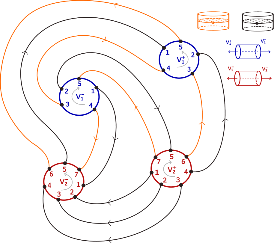
Figure 1. ${\mathscr{H}}$-graph of $P^{3}$

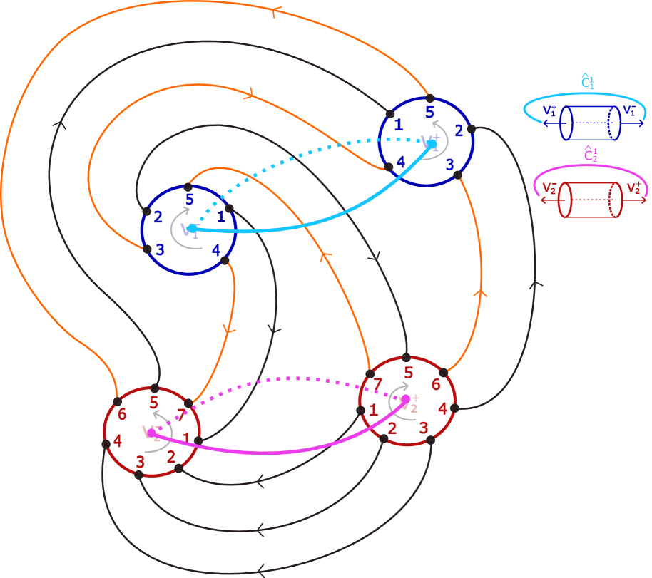
Figure 2. Generators

In order to obtain a finite presentation of $H_{1}(P^{3};\mathbb{Z})$ as described in the proof of Proposition 10, we start by extending the cores of the two 1-handles into ${\mathcal{H}}_{0}$ to obtain the generators $A_{1}=[\hat{C}^{1}_{1}]$ and $A_{2}=[\hat{C}^{1}_{2}]$ (See Figure 2). Now, we have two relators $R_{1}=[\partial E_{1}]$ and $R_{2}=[\partial E_{2}]$ associated to the 2-handles colored orange and black, respectively, where $[\partial E_{i}]=r_{1i}A_{1}+r_{2i}A_{2}$ for $i=1,2$. Keeping in mind that $\hat{C}_{1}^{1}\overset{a}{\cap}C^{1}_{1}=1$ and $\hat{C}_{2}^{1}\overset{a}{\cap}C^{1}_{2}=1$, we have

$$R_{1} =-A_{1}+2A_{2}$$

$$R_{2} =-2A_{1}+3A_{2}$$

Now, since $P^{3}$ has trivial first homology, then $A_{i}=[\hat{C}_{i}]=0$ for $i=1,2$ and so each $A_{i}$ bounds a surface. In terms of the relators $R_{1}$ and $R_{2}$, we have the following

$$A_{1} =x_{1}R_{1}+y_{1}R_{2}=x_{1}(-A_{1}+2A_{2})+y_{1}(-2A_{1}+3A_{2})=(-x_{1}-2y_{1})A_{1}+(2x_{1}+3y_{1})A_{2}$$

$$A_{2} =x_{2}R_{1}+y_{2}R_{2}=x_{2}(-A_{1}+2A_{2})+y_{2}(-2A_{1}+3A_{2})=(-x_{2}-2y_{2})A_{1}+(2x_{2}+3y_{2})A_{2}$$

which results in the following two systems

$$-x_{1}-2y_{1} =1 -x_{2}-2y_{2} =0$$

$$2x_{1}+3y_{1} =0 2x_{2}+3y_{2} =1$$

Once solved, we get that

$$x_{1} =3 x_{2} =2$$

$$y_{1} =-2 y_{2} =-1$$

and so

$$A_{1} =3R_{1}-2R_{2}$$

$$A_{2} =2R_{1}-R_{2}$$

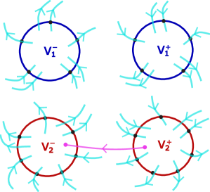
Figure 3. $A_{2}\sqcup L_{E_{2}}$

Now, $A_{2}$ is not balanced. The extension link needed to balance $A_{2}$ is $L_{E_{2}}=(\bigsqcup_{2}-\partial E_{1})\bigcup(\partial E_{2})$. By construction, $A_{2}\sqcup L_{E_{2}}$ will be balanced (see Figure 3) and, by Proposition 9, will bound an oriented surface contained in the 0- and 1- handles of $P^{3}$.

Figure 5 shows $L_{E_{2}}$ projected onto ${\mathscr{H}}\setminus V_{i}^{\pm}$. In order to identify the surface that $A_{2}\sqcup L_{E_{2}}$ bounds, we add in pairing paths as shown in Figure 5.

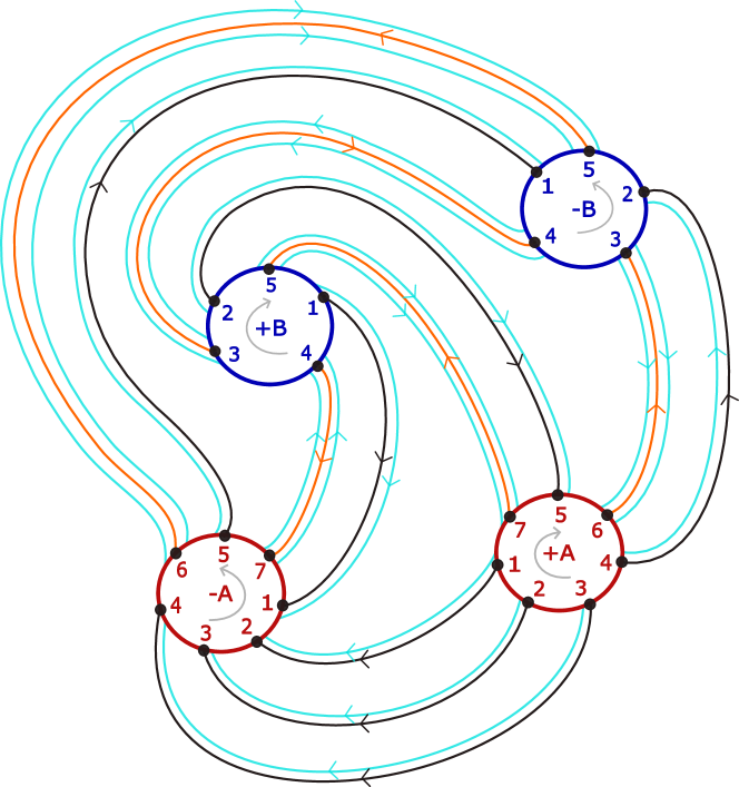
Figure 4. $L_{E_{2}}\subset{\mathscr{H}}\setminus V^{\pm}_{i}$

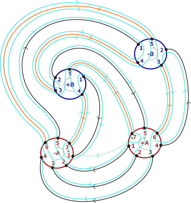
Figure 5. Pairing paths for $L_{E_{2}}$

After resolving one crossing, shown in Figure 7, the union of $A_{2}\sqcup L_{E_{2}}$ along with the pairing paths will correspond to an oriented unlink projection with spanning disks shown in Figure 7. A rectangular 2-disc band is attached, in the associated 1-handle, to each corresponding pair of pairing paths. The resulting surface will be oriented, in normal position, and contained in the 0- and 1- handles of $P^{3}$. Lastly, since each extension disc used in the construction is contained in $P^{3}\setminus A_{2}$, each boundary component of $L_{E_{2}}$ can be capped off by an extension disc. The result will be an oriented surface, $\Sigma_{E_{2}}^{2}$, in normal position having $A_{2}$ as its boundary.

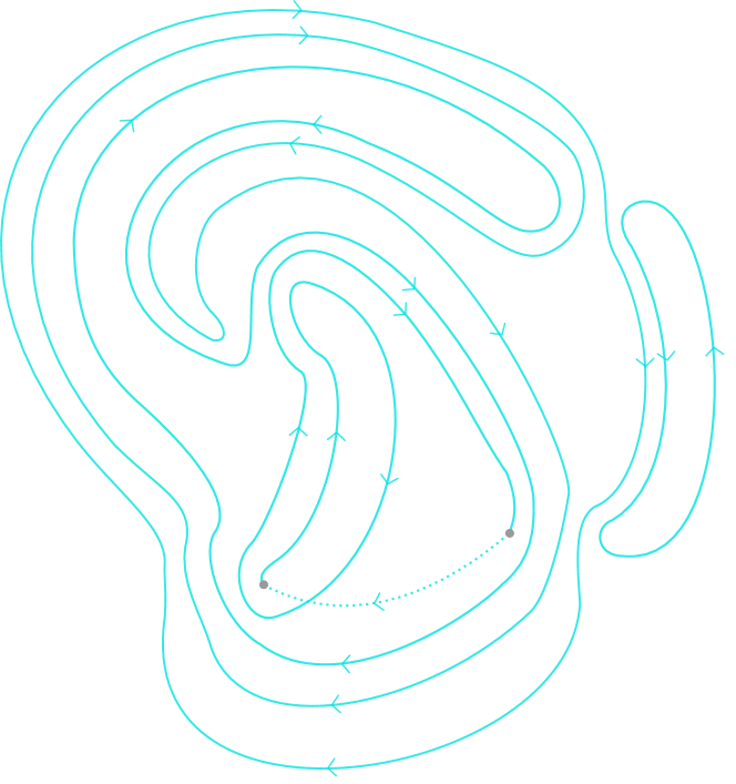
Figure 6. Seifert Circles for $A_{2}$

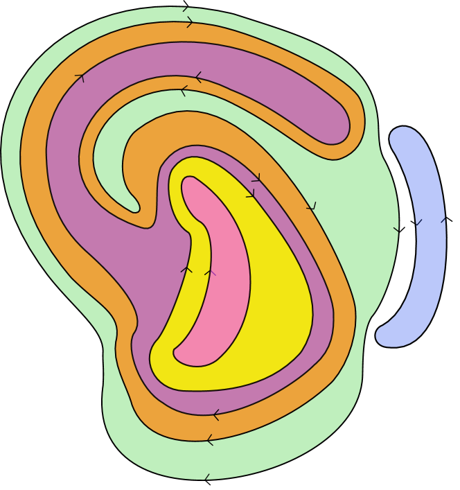
Figure 7. Disks in ${\mathcal{H}}_{0}$ for $A_{2}$

The Euler characteristic could be calculated by computing the following:
$\chi(\Sigma_{E_{2}}^{2})=\sum_{i=0}^{2}(-1)^{i}(\#\textrm{ of }i-\textrm{handles})=6-10+3=-1.$
Since $\Sigma_{E_{2}}^{2}$ has one boundary component, namely $A_{2}$, this surface is one homeomorphic to a once-punctured torus.

We repeat the same procedure in order to identify the surface that $A_{1}$ bounds. Since $A_{1}$ is not balanced, the extension disc needed to balance it is $L_{E_{1}}=(\bigsqcup_{3}-\partial E_{1})\bigcup(\bigsqcup_{2}\partial E_{2})$. Therefore, $A_{1}\cup L_{E_{1}}$ will be balanced and the projection of $L_{E_{1}}$ onto ${\mathscr{H}}\setminus V_{i}^{\pm}$ can be seen in Figure 9. We add pairing paths as shown in Figure 9.

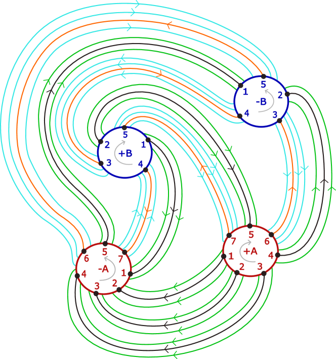
Figure 8. $L_{E_{1}}\subset{\mathscr{H}}\setminus V^{\pm}_{i}$

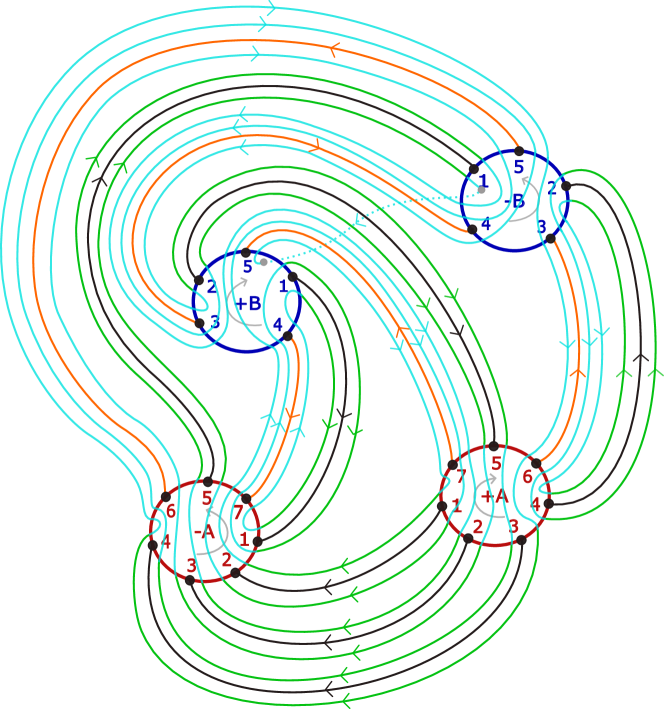
Figure 9. Pairing paths for $A_{1}$

After resolving multiple crossings as seen in Figure 11, the union of $A_{1}\sqcup L_{E_{1}}$ along with the pairing paths will correspond to an oriented unlink projection with spanning disks shown in Figure 11. After attaching the corresponding rectangular 2-disc bands, the resulting surface will be oriented, in normal position, and contained in the 0- and 1- handles of $P^{3}$. After capping off each boundary component of $L_{E_{1}}$ with an extension disc, the resulting surface, $\Sigma_{E_{1}}^{2}$, will be in normal position having $A_{1}$ as its boundary. The surface will have Euler characteristic $\chi(\Sigma_{E_{1}}^{2})=11-23+5=-7.$

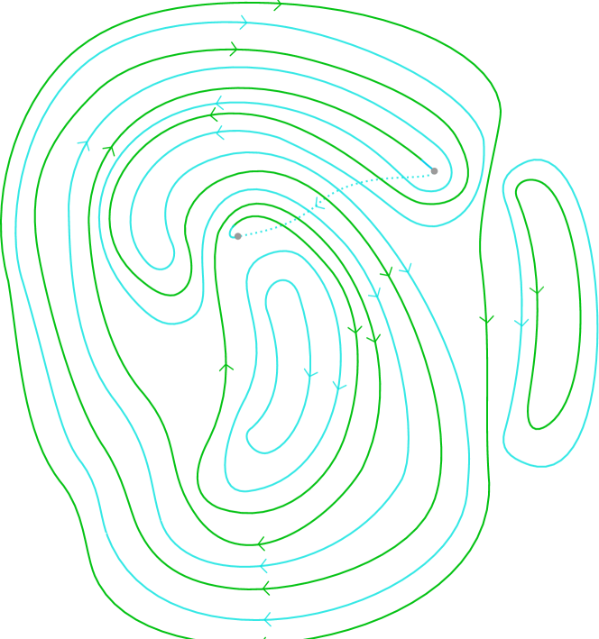
Figure 10. Seifert Circles for $A_{1}$

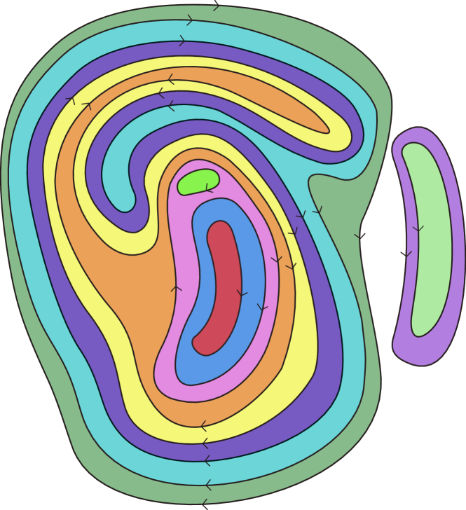
Figure 11. Discs in ${\mathcal{H}}_{0}$ for $A_{1}$

4. Constructing a Heegaard graph from framed links.

The Heegaard graph similar to the one in §3 for the Poincaré Homology Sphere is the starting point for performing our generalization of Seifert’s algorithm. That Heegaard graph comes from D. Rolfsen’s “one-time” procedure that starts with $+1$ Dehn surgery on the right-handed trefoil knot and, through a sequence of geometric manipulations, decomposes the $3$-manifold into the corresponding handlebody [4]. It is true that we have a ready supply of integral homology spheres coming from $\pm 1$ Dehn surgery on links in $S^{3}$. But, to advance the project of studying knots and links in an arbitrary $3$-manifold using link projections in the Heegaard graph, we will need to systematize Rolfsen’s original one-time procedure. To this end, we now describe how a plat presentation of a specified framed link is readily transformed into a Heegaard graph.

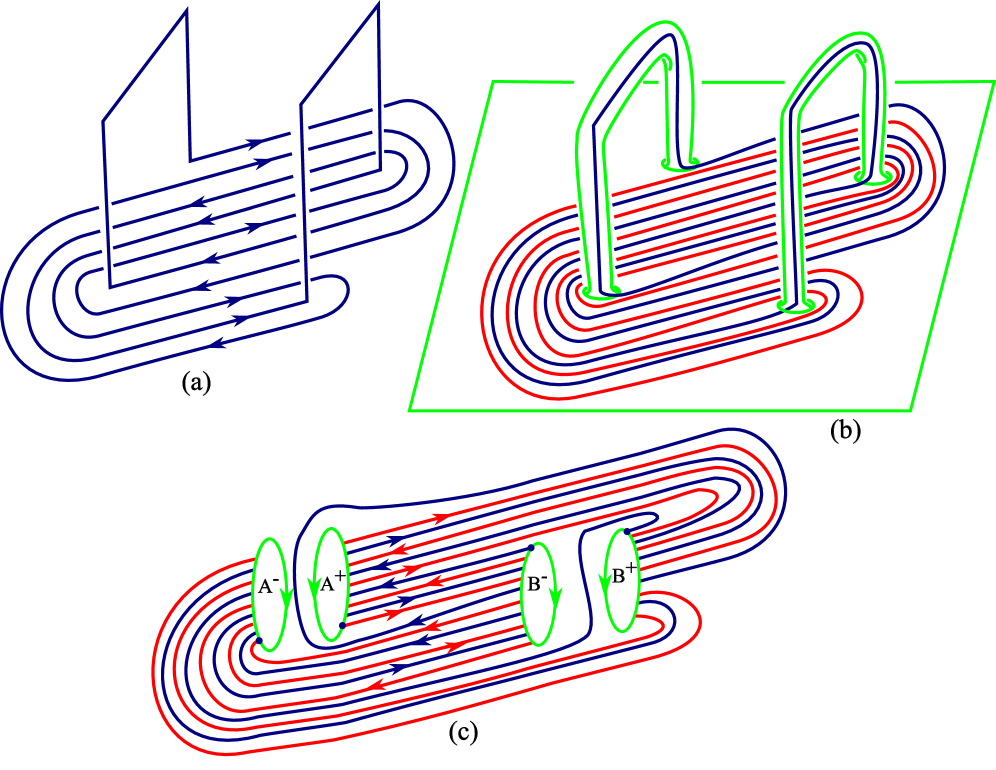
Figure 12. In (a) we depict a plat presentation with $2$ arcs in a plane which are connected above by $2$ bridges. In (b) we depict the associated genus $2$ splitting surface with $2$ curves (red and blue) that are where the two $2$-handles are attached. In (c) we depict the associated Heegaard graph.

Our procedure is inspired by the initial figure in [2] which we replicate in Figure 12(a). Specifically, every link $L$ in $S^{3}$ has a flat plat presentation—a decomposition of $L$ into $n$ pairwise disjoint simple arcs in a sphere (or plane) with $n$ (unknotted) bridges positioned “above” the sphere connecting the planar arcs together to form the link. Figure 12(a) illustrates a flat plat presentation for the figure eight knot. There are $2$ simple arcs in the sphere which are connected by $2$ bridges above the sphere. It is convenient to depict the $2$ bridges in a rectangular fashion—two vertical edges and one horizontal edge. This confirms that the bridges are unknotted with respect to the sphere by giving readily identifiable unknotting discs for the bridges—the embedded discs that would be swiped-out by an isotopy that takes the bridges to arcs embedded in the sphere.

Our procedure for producing a Heegaard graph of the homology sphere produced by $\pm 1$ Dehn surgery on the components of $L$ first requires that we take a flat plat presentation of $L$ and construct a solid handle body of genus $n$, $H_{n}$. We will denote the boundary of $H_{n}$ by $\Sigma_{n}$.

Once we have specified $H_{n}$ we need to go in two different directions. The first direction is identifying $n$ characteristic curves in $\Sigma_{n}$ where $2$-handles will be attached to $H_{n}$. The second direction is giving a decomposition of $H_{n}$ into a single $0$-handle with $n$ $1$-handles attached.

For the first direction, in order to obtain the correct framing for the $n$ characteristic curves, it is convenient to require that the writhe of each component of $L$ correspond to the Dehn surgery that is being applied. For example, in Figure 12(a) the writhe of the flat plat projection of the figure eight is readily calculated as $+1$. This will position us to produce a Heegaard graph of a homology sphere that is the result of $+1$ Dehn surgery on the figure eight. That such a flat plat presentation always exists is a straight forward argument that we leave to the reader.

Identifying $H_{n}$ and $\Sigma_{n}$. We attach to the sphere $n$ annular tubes, one for each bridge of the plat presentation—one can think of an annular tube as being the boundary of a regular neighborhood of a bridge. The resulting genus $n$ surface is $\Sigma_{n}$. Due to the unknotted nature of the $n$ bridges, it is immediate that $\Sigma_{n}$ is the boundary of a solid handle body positioned “above” the sphere. Figure 12(b) illustrates the associated genus $2$ surface, $\Sigma_{2}$. Our viewpoint is one where we are positioned inside $H_{2}$.

Identifying characteristic curves in $\Sigma_{n}$. Our choice of $n$ characteristic curves on $\Sigma_{n}$—all of which are non-separating curves—starts with the components of $L$. $\Sigma_{n}$ has the property that the components of $L$ are non-separating simple closed curves in $\Sigma_{n}$. We observe that the number of components, $|L|\leq n$. If $|L|=n$ then $L\subset\Sigma_{n}$ is the required collection of characteristic curves.

If $|L|<n$ then there will be at least $k=n-|L|$ planar arcs, $\{a_{1},\cdots a_{k}\}$ of the initial flat plat presentation of $L$ that satisfy the following property $\star\star$: the two endpoints of $a_{i}$ are not attached to the same bridge. For each such planar arc, we consider the boundary of a regular neighborhood, $\{c_{1},\cdots,c_{k}\}$, all of which are in the sphere that is utilized in our flat plat presentation. It is readily seen that, except when $n=2$, the $c_{i}{\rm{}^{\prime}s}$ are in distinct, isotopic classes. As such, each $c_{i}$ is positioned away from where we attach the $n$ annular tubes used in the formation of $\Sigma_{n}$. By property $\star\star$, each resulting $c_{i}$ in $\Sigma_{n}$ will be a non-separating curve. Our collection of characteristic curves is then all the components of $L$ in $\Sigma_{n}$ plus a choice of some number of the $c_{i}{\rm{}^{\prime}s}$ so as to give a complete count of $n$ non-separating curves.

Referring the reader to Figure 12(b), the red curve is obtained by looking back at Figure 12(a) and taking the boundary of a regular neighborhood of the planar arc that has the two endpoints, $NE$ and $SW$ (using compass referencing). Then the two characteristic curves consist of this red curve and the knot that is in blue.

Decomposition of $H_{n}$ into a $0$-handle with $n$ $1$-handles. We will want to see this handle body as being decomposed into a single $0$-handle with $n$ $1$-handles attached. Our viewpoint will now be one where we are positioned in the $0$-handle. To specify the $1$-handles we need only specify the boundary of $n$ co-cores. These will come from the $n$ discs which characterize the $n$ rectangular bridges as being unknotted.

Using the two obvious unknotting discs for the two rectangular bridges of Figure 12(b), the reader should now be able to interpret the handle structure of this illustration. Away from the two annular tubes, one is inside the unique $0$-handle. When one travels underneath either tube, one is traveling through a $1$-handle.

Producing the Heegaard graph. With the $0$-handle and $1$-handle structure of $H_{n}$ defined, we are now in a position to produce the associated Heegaard graph. This is done by splitting $H_{n}$ along the $n$ $1$-handle co-cores to produce a planar graph. The vertices of this graph will be the pairs of discs associated with the co-cores. The edges of this graph correspond to splitting the characteristic curves along their intersections with the $1$-handle co-cores.

Figure 12(c) depicts this splitting procedure coming from our flat plat presentation of the figure eight. It is a straight forward task to repeat the homological calculation of §3 and see that the $+1$ writhe framing of Figure 12(a) yields an integral homology sphere.

5. Uses of a new tool

Generalized Alexander Polynomial–One obvious direction for a generalized Seifert surface algorithm is to carry out each feature of Seifert’s original program [5] except now in the setting of an arbitrary homology sphere. Specifically, coming from the $\pi_{0}$-regular projection of an oriented link in an ${\mathscr{H}}$-graph, use the associated Seifert surface in pseudo-normal position to give an effective procedure for calculating an associated “Seifert matrix”. Such a (generalized) Seifert matrix will yield an associated “Alexander polynomial”. This in fact is the current direction of the first author’s work. The goal is to follow the road map that was laid out in [5] for initially determining the scope of the behavior of such link polynomials.

Minimal genus spanning surfaces—A second obvious line of inquiry comes from the algebraic calculation in the proof of Proposition 10. Specifically, there are “non-trivial solutions” to equation (2.2) coming from the fact that one can add in cancelling extension discs—extension discs of opposite orientation. Such an addition of extension discs would contribute parallel components to $L_{E}$ that are oppositely oriented. However, this adds to the possible choices of the pairing paths used in the proof of Proposition 9. So how does the genus of the Seifert surface behave when cancelling extension discs are thrown in? A reasonable conjecture is that minimal genus is achieved when $|L_{E}|$ is minimal.

References

- [1] Nikolai Saveliev, Lectures on the Topology of 3-Manifolds, De Gruyter textbook, 1991 Mathematics Subject Classification: 57-01; 57-02, 57 https://www.overleaf.com/project/620422ac30aa347b0223b845
- [2] Allan Hatcher and William Thurston, Incompressible surfaces in 2-bridge knot complements, Invent. Math. 79, 225–246 (1985). https://doi.org/10.1007/BF01388971
- [3] Robion C. Kirby, The Topology of 4-Manifolds, Lecture Notes in Mathematics, 1989, Vol. 1374.
- [4] Dale Rolfsen, Knots and Links, AMS Chelsea Publishing; American Mathematical Society, 1976, Vol. 346.
- [5] Herbert Seifert, Über das Geschlecht von Knoten, Mathematische Annalen 110 (1935), no. 1, 571–592.