Can LLMs Solve Longer Math Word Problems Better?

Abstract

Math Word Problems (MWPs) are crucial for evaluating the capability of Large Language Models (LLMs), with current research primarily focusing on questions with concise contexts. However, as real-world math problems often involve complex circumstances, LLMs’ ability to solve long MWPs is vital for their applications in these scenarios, yet remains under-explored. This study pioneers the exploration of Context Length Generalizability (CoLeG), the ability of LLMs to solve long MWPs. We introduce Extended Grade-School Math (E-GSM), a collection of MWPs with lengthy narratives. Two novel metrics are proposed to assess the efficacy and resilience of LLMs in solving these problems. Our examination of existing zero-shot prompting techniques and both proprietary and open-source LLMs reveals a general deficiency in CoLeG. To alleviate these challenges, we propose distinct approaches for different categories of LLMs. For proprietary LLMs, a new instructional prompt is proposed to mitigate the influence of long context. For open-source LLMs, a new data augmentation task is developed to improve CoLeG. Our comprehensive results demonstrate the effectiveness of our proposed methods, showing not only improved performance on E-GSM but also generalizability across several other MWP benchmarks. Our findings pave the way for future research in employing LLMs for complex, real-world applications, offering practical solutions to current limitations and opening avenues for further exploration of model generalizability and training methodologies.

1 Introduction

Math word problems (MWPs) [1] are mathematical questions presented in natural language, demanding delicate reasoning for solving. With the flourish of large language models (LLMs) [2, 3, 4, 5], the math reasoning ability measured on MWPs benchmarks has emerged as a critical evaluation metric to assess the overall capability of these models. The representative benchmarks for MWP include GSM8K [6], which is characterized by concise descriptions in a few sentences. However, this setting differs from real-world scenarios, where MWPs usually come with longer context. [7] suggests that extensive contexts might hinder rather than facilitate the mathematical reasoning process. This observation raises an important question: Do LLMs exhibit a performance degradation in solving long MWPs? If so, how can we improve LLMs performance on these long MWPs?

To answer these questions, the chain-of-thought [8] (CoT) is conducted on the GSM8K bechmark and questions are segregated based on the accuracy of CoT predictions. Rigid statistical hypothesis testing has revealed significant evidence suggesting that LLMs exhibit decreased performance on MWPs with long context (see Section 2.1). In order to further investigate how are different LLMs affected by lengthy contexts of MWPs, we construct the Extended Grade-School Math (E-GSM), a benchmark comprising MWPs with extended context derived from GSM8K, and two novel evaluation metrics. E-GSM maintains minimal alterations to the conditions and the order of conditions while extending the contextual information of the original problem. We investigate seven proprietary and 20 open-source LLMs, along with three state-of-the-art zero-shot prompts on E-GSM. Our results indicate that the Context Length Generalization (CoLeG) of these LLMs, the ability for LLMs to do math reasoning in a long context, is limited, particularly with longer MWPs.

To alleviate this issue, we propose two different strategies for proprietary and open-source LLMs, respectively. For proprietary LLMs, inspired by cognitive load theory [9], we develop Condition-Retrieving Instruction (CoRe) prompting technique, which encourages LLMs to retrieve problem conditions first and then apply different reasoning modules. For open-source LLMs, we suggest incorporating extension as an auxiliary task during fine-tuning. We validate our strategies on E-GSM, and several other MWP benchmarks such as MAWPS [10], SVAMP [11], and GSM-IC [12], demonstrating their effectiveness and generalizability.

We summarize our main contributions as follows:

1. We construct the E-GSM dataset, comprising MWPs with longer contexts. Comprehensive experiments on both proprietary and open-source LLMs reveal that math reasoning abilities of LLMs are significantly affected by long context.

2. We develop a new instructional prompt named CoRe for proprietary LLMs , which can significantly improve CoLeG and accuracy of LLMs on E-GSM.

3. We propose to use extension as an auxiliary task to fine-tune open source LLMs and release our fine-tuning dataset comprising 65K CoT data.

4. CoRe and extension have demonstrated their strong generalization on several MWP benchmarks.

The ability of LLMs to solve long MWPs is important for their application in real-world scenarios. Our evaluation indicates that long MWPs will heavily degrades the math reasoning ability of LLMs, and further experiments demonstrate the effectiveness and generalizability of our proposed methods for both proprietary and open-source LLMs. Our findings provides valuable insights and directions for future research on using LLMs to solve math problems.

2 The E-GSM Dataset

2.1 LLMs Struggle to Answer Math Word Problems with Longer Context

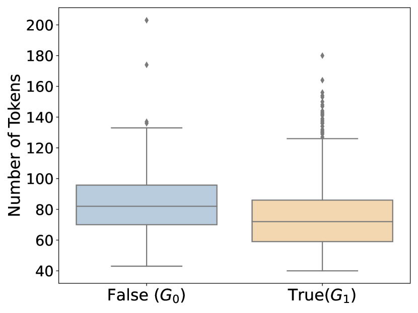
Figure 1: The visual comparison suggests the number of tokens in $G_{0}$ is larger than $G_{1}$, with Mann-Whitney U test suggesting the significance of these differences. This implies that LLMs struggle to solve longer MWPs, which is similar to humans.

To explore whether the performance of LLMs in mathematical reasoning is adversely affected by longer textual contexts, similar to human performance, we conducted an experiment on GSM8K using CoT with GPT-3.5-turbo as the representative. The experiment employed the 8-shot demonstrations provided by [8], and the complete prompt can be found in Appendix D. We can compare the answers generated by LLMs with the ground-truth answers and then divide the examples into two groups based on accuracy: the correct answers group $G_{0}$ and the incorrect answers group $G_{1}$.

We want to study whether there exists a significant difference in the problem length, characterized by the number of tokens, between these two categories. We hypothesize that the lengths of the problem descriptions for these two groups are from different distributions, denoted $X$ and $Y$. As illustrated in Figure 1, the distributions between $X$ and $Y$ are quite different. To conduct a rigorous analysis, we apply the one-sided Mann-Whitney test [13]:

$$H_{0}:\ P(X<Y)=P(X>Y)\leftrightarrow H_{1}:\ P(X<Y)>P(X>Y).$$

The results are reported following [14]: There is significant evidence indicating that the number of tokens in $G_{0}$ is less than in $G_{1}$ with $U=141565,P=0.0000$, which suggests LLMs perform better on short MWPs than longer ones, similar to human problem solvers.

To address the potential condounding factors, we further explore whether longer problem correlates with increased problem difficulty. We utilize the number of steps required by GPT-3.5-turbo to solve the problems as a proxy for problem difficulty [15, 8], denoted by $S$, a discrete random variable with $k$ levels. We assumed that the number of problem tokens is denoted by $T$. To analyze this relationship, we consider the following linear model:

$$\text{log}\,T=\beta_{0}+\beta_{1}S_{1}+\beta_{2}S_{2}+\ldots+\beta_{k-1}S_{k-1}+\varepsilon,$$

where $\beta_{i}$ is the coefficient corresponding to the difference in the dependent variable associated with the $i$-th level of $S$ to the reference category. The logarithmic transformation of $T$ is to ensure homogeneity of variance, confirmed by a Levene’s test [16] for homogeneity of variance ($P=0.1518$). Subsequently, we proceeded with a contrast test [17]:

$$H_{0}:\ C\cdot\beta=0\leftrightarrow H_{1}:\ C\cdot\beta\neq 0,$$

where $C$ is the contrast coefficients (Appendix B.5), and $\beta=[\beta_{1},...,\beta_{k-1}]$. The results indicate insufficient statistical evidence to confirm the linear contrast ($F=1.9158,P=0.1476)$, suggesting insufficient evidence that a direct relationship exists between the problem length and its difficulty.

These findings eliminate the potential confounding factor that longer questions are more difficult and compellingly indicate that, similar to human solvers, LLMs may be lost in longer MWPs.

2.2 Dataset Creation

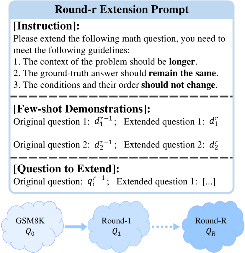
Figure 2: E-GSM creation process and prompt template for extension.

To conduct a more comprehensive analysis of CoLeG across a range of LLMs, we have created E-GSM as a testing ground. Our approach leverages GPT-4-turbo to extend the original GSM8K benchmark. Specifically, we primarily construct the data that should meet the following three requirements: 1) The context of problems should be longer. 2) The ground-truth answers should remain the same. 3) The conditions and their order should not change. This section will detail the construction process.

Initial trails revealed that generated questions were only slightly longer than their original questions, and GPT-4-turbo failed to achieve a specified token length as set out in the instructions. To overcome this issue and facilitate the extension of math problems into more elaborate contexts, we adopted a sequential, iterative strategy. The process commences with the GSM8K [6] test set.. During the $r$-th iteration, the $i$-th question from the preceding iteration $(r-1)$, denoted as $q_{i}^{r-1}\in Q_{r-1}$, is extended using 2-shot demonstrations with GPT-4-turbo. Following the expansion in the $r$-th round, quality control is performed to ensure quality (see Section 2.3), resulting in the refined set of extended problems, $Q_{r}$. The prompt structure, along with the entire extension process, is depicted in Figure 2. Human evaluation and heuristic methods are conducted to ensure the quality of LLM extended questions (Section 2.3).

As the expansion progresses, we observe a gradual increase in the length of questions. The average tokens for MWPs in each stage are presented in Table 1. In the later phases, a deceleration in the rate of increase in the number of tokens is observed, leading us to end at $R=4$. As a result, our E-GSM incorporates extended problems from all rounds $\cup_{r=1}^{R}Q_{r}$. Examples are provided in Appendix A.1.

2.3 Quality Control

Round	$Q_{0}$	$Q_{1}$	$Q_{2}$	$Q_{3}$	$Q_{4}$
#Tokens	77.0	192.2	301.5	363.5	385.7
#Questions	1319	1195	1143	1102	1068

Table 1: The average tokens of E-GSM dataset where the number of tokens is returned by GPT-4-turbo and the number of questions in each round of extension.

After obtaining extended questions, we have to ensure they meet our requirements mentioned in Section 2.2. We perform quality control process in the following two steps: 1) We apply human evaluation on a subset of E-GSM to precisely assess the quality of questions. Evaluation results shows that most of questions possess excellent quality. 2) We devise two heuristics to automatically filter undesired extended questions of the entire dataset.

Fifty seed questions are randomly selected from GSM8K and all questions derived from these selected questions are manually inspected (200 in total, with 50 seed problems per round). Three annotators assess the quality of the extended questions based on specific criteria and assign a quality level to each question. The final quality level is determined through majority voting. The judging criteria for each quality level and several examples are provided in Appendix A.2. Our evaluation finds that 185 of the 200 extended problems are of excellent quality, 4 are good, and 11 are poor.

Due to resource constraints, it is impractical to conduct human evaluations across the entire dataset. Instead, we employ two heuristics to eliminate problematic instances. We guarantee that these methods will effectively detect all substandard examples within our selected questions and then apply them to the full dataset to ensure its quality.

First, we ensure that the extended variant faithfully retains information from the seed question through computing entailment score between the two. For the $i$-th seed question $q_{i}^{0}$ and its associated extended variants $q_{i}^{1},...,q_{i}^{R}$, we derive a score $S_{i}^{r}=ENT(q_{i}^{r},q_{i}^{0})$ to evaluate the informational equivalence. More specifically, we adopt the out-of-box entailment model [18] to calculate $S_{i}^{r}$ (see Appendix A.3). A small $S_{i}^{r}$ can suggest a potentially unsatisfactory extension, leading to the exclusion of the question $q_{i}^{r}$ if $S_{i}^{j}<\tau_{1},\text{for any}\ j\leq r$. Obviously, $Q_{r}\subseteq Q_{r-1}$ after filtration.

Second, we consider an extended variant unsolvable and filter it out if it cannot be addressed by proficient LLMs using various prompting methods. More concretely, GPT-4-turbo and Claude-3-opus with 6 different prompting methods are used to generate solutions for each question (see Section 4.1), and questions whose accuracy across 12 solutions is less than $\tau_{2}$ are discarded.

From human evaluation of a subset, we can see that most of our extended questions are of excellent quality. We adjust the thresholds $\tau_{1}$ and $\tau_{2}$ based on human evaluation results, successfully filtering out examples of poor quality by setting $\tau_{1}=\tau_{2}=0.2$. The number of questions retained in each round is shown in Table 1.

2.4 Evaluation of Efficacy and Robustness on E-GSM

We propose two metrics to evaluate the performance of LLMs on E-GSM from two different angles: efficacy and robustness. For efficacy, our goal is to check whether a question and all its corresponding variants can be consistently solved, thereby evaluating the model’s capability to accurately solve the same question regardless of variations in context length and circumvanting potential randomness. For robustness, the relative performance drop of the accuracy from $Q_{0}$ to $Q_{R}$ is used. For a given question $q$, its ground-truth answer is denoted by $\text{gt}(q)$, and the answer generated by the method $\mathcal{M}$ is represented as $\mathcal{M}$$(q)$. The following metrics are considered:

Round-$r$ accuracy $\text{Acc}_{r}(\mathcal{M})$ = $\text{Acc}(\mathcal{M};Q_{r})$ is defined as the average accuracy of method $\mathcal{M}$ on the set of problems $Q_{r}$.

$$\text{Acc}(\mathcal{M};Q_{r})=\frac{\sum_{q\in Q_{r}}\mathbb{I}[\mathcal{M}(q)=\text{gt}(q)]}{|Q_{r}|},$$

where $|\cdot|$ denotes the number of questions in a set.

CoLeG-E quantifies the efficacy of CoLeG, which is defined as the averaged accuracy of $\mathcal{M}$ to solve a seed question and all its corresponding extension variants.

$$\text{{CoLeG-E}}(\mathcal{M})=\frac{\sum_{q_{i}^{R}\in Q_{R}}\left[\wedge_{r=1}^{R}\mathbb{I}[\mathcal{M}(q_{i}^{r})=\text{gt}(q_{i}^{r})]\right]}{|Q_{R}|},$$

indicating that CoLeG-E evaluates the proportion of original problems that can be consistently solved across all levels of extended context.

CoLeG-R assesses the robustness facet of CoLeG, which is characterized by the relative accuracy drop rate on $Q_{R}$ compared to the performance on initial questions $Q_{0}$:

$$\text{{CoLeG-R}}(\mathcal{M})=1-\frac{\text{Acc}_{0}(\mathcal{M})-\text{Acc}_{R}(\mathcal{M})}{\text{Acc}_{0}(\mathcal{M})}.$$

3 Methodology

In this section, we detail our novel approaches aimed at enhancing CoLeG and describe our experimental setup. Given that access to the model weights of proprietary LLMs is restricted, we have developed a new instructional prompt, to increase the abilities of LLMs in solving long MWPs (Section 3.1). For open-source LLMs, we introduce a new data augmentation technique, extension, to boost CoLeG by enriching the training data (Section 3.2).

3.1 Condition-Retrieving Instruction for Proprietary LLMs

Although proprietary LLMs exhibit strong math reasoning capability, they are still negatively impacted by long context in solving MWPs. Through our delicate inspection of their generated solutions, we observed that LLMs with conventional prompting methods often struggle to extract relevant conditions from extensive contexts. Drawing inspiration from cognitive load theory [9], which suggests that humans are only conscious of the contents that exist in a limited-size working memory and all other information is hidden until it is swapped into working memory, we suppose that a similar mechanism exists for LLMs in solving MWPs. Long MWPs make the “LLMs’ working memory” saturated by story details, and missing key conditions that are essential to solve the problem. To alleviate this issue, we propose a novel Condition-Retrieving Instruction (CoRe), which begins by guiding LLMs to identify the conditions and ultimate objective of the given problem, making sure “LLMs’ working memory” is filled with essential conditions rather than story details, and then apply other reasoning modules to solve the original problem. Any zero-shot prompting methods can serve as reasoning modules of CoRe. As shown in Figure 3, LLMs with 0-shot CoT miss “she adds 15 milliliters of cream after the coffee is cooled”, not getting the correct answer. In contrast, with the help of CoRe, LLMs could precisely parse conditions and the ultimate goal from the original problem, and accurately deduce the numerical answer, showcasing the effectiveness of our instruction. For more comparative examples, please refer to Appendix E.

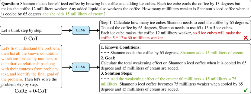
Figure 3: A comparison between solving a lengthy math problem with 0-CoT and CoRe + 0-CoT.

3.2 Extension as an Auxiliary Task for Open-source LLMs

Extracting information from a lengthy context to perform mathematical reasoning is essential for real-world tasks. However, current LLMs have significantly lower accuracy in longer MWPs (Section 2.1), motivating us to extend longer questions to improve reasoning capability. We can generate longer MWPs using extension technique introduced in Section 2.2. The quality control heuristic in Section 2.3 can be applied to filter out extended questions with poor quality. The new questions and their generated reasoning paths are collected as augmented data:

$$\mathcal{D}_{r}=\{(q_{i}^{r},e_{ij}^{r},a_{ij}^{r}):a_{i}^{r}=\text{gt}(q_{i}^{r});i=1,2,...,N_{r};j=1,2,...,K_{ij}^{r}\},$$

where $r$ denotes the round of extension, $i$ is the index of questions, $e_{ij}^{r},a_{ij}^{r}$ are augmented reasoning path and corresponding answer for the $i$-th question in $r$-th round of extension $q_{i}^{r}$, $\text{gt}(\cdot)$ is the ground-truth answer, $N_{r}$ is the number of questions left in $r$-th round after quality control, and $K_{ij}^{r}$ is the number of augmented CoT paths for $q_{i}^{r}$.

We fine-tune an LLM (parameterized by $\boldsymbol{\theta}$) on $\mathcal{D}=\mathcal{D}_{0}\cup\mathcal{D}_{1}$ by maximizing the log likelihood of the reasoning path and corresponding answer conditioned on the question. The specific loss we used during supervised fine-tuning is given as follows:

$$\mathcal{L}(\boldsymbol{\theta})=\sum\nolimits_{(q,r,a)\in\mathcal{D}}\log\mathbb{P}(r,a\mid q;\boldsymbol{\theta}).$$

3.3 Experimental Setup

Investigated LLMs. For the investigation of prompting methods, we include mainstream proprietary LLMs such as GPT-4 [4], GPT-3.5-turbo, GPT-3.5-instruct, GLM-3 [19], Gemini-pro [20], and Claude-3. For fine-tuning open-source LLMs, our study encompasses LLaMA-2 [21], LLaMA-3 across different model scales, Mistral-7B [22] and specialized mathematical models across different base models and model sizes, including WizardMath [23], MAmmoTH [24], MetaMath [25], and Llemma [26]. More detailed descriptions of these LLMs can be found in Appendix B.1.

Investigated Prompting Techniques. To negate the influence of few-shot demonstrations, we explore zero-shot prompting techniques, including zero-shot CoT (0-CoT) [27], Plan-and-Solve (PS)[28], and a variant of PS (PS+). A brief introduction of these prompts are covered in Appendix D. Additionally, we explore the role of self-consistency (SC) [29] in improving CoLeG of LLMs. For our implementation of SC, we generate 5 responses using a sampling temperature of $0.7$.

SFT Dataset. To generate our augmented dataset, We generate five reasoning paths for each question in the training set with GPT-3.5-turbo and remove any paths that led to incorrect final answers. Apart from 7,473 annotated examples available in GSM8K training set, we get $\mathcal{D}_{0}$ that incorporate 38,507 valid CoT data points and $\mathcal{D}_{1}$ that includes 26,422 CoT data for extended quesitons. The entire training set, represented as $\mathcal{D}=\mathcal{D}_{0}\cup\mathcal{D}_{1}$, incorporates 64,929 CoT data. Appendix B.2 shows the input-output formats of the SFT data and examples from both $\mathcal{D}_{0}$ and $\mathcal{D}_{1}$. We also collect $\mathcal{D}_{2}$ of 24,147 CoT data to study the effect of scaling up the SFT data (see Section C.4).

SFT Setup. Multiple open-source LLMs, differing in scale and base models, are fine-tuned on $D$. The fine-tuning is carried out over 3 epochs and the results are reported using 0-CoT with the vLLM library. All evaluations adhere to the same 0-CoT instruction set to ensure consistency. To account for the potential influence of random variations during the training process, we include the performance trends throughout the entire training period in Appendix C.1. Furthermore, comprehensive details regarding the training and inference parameters can be found in Appendix B.4.

Answer Extraction. To report the results, we use GPT-3.5-turbo to extract the final answers in case that responses may not follow the desired format. Our answer extraction methods successfully get the final answer $99.8\%$ and details are provided in Appendix B.3. The specific designs for these zero-shot prompts are delayed to Appendix D, and the outcomes are presented in Section 4.1.

4 Results and Analysis

4.1 Prompting Results of Proprietary LLMs

We compare the performance of different proprietary LLMs with various zero-shot prompting techniques on E-GSM. Representative results are shown in Table 2, and full results are given in Appendix C.2. From Table 2 we have following conclusions:

LLMs	CoLeG-E	CoLeG-R	$\text{Acc}_{0}$	$\text{Acc}_{4}$
Claude-3-opus
PS	74.81	84.07	95.45	80.24
+ CoRe	78.00	87.07	95.60	83.24
PS+	75.00	84.79	95.30	80.81
+ CoRe	78.28	86.01	95.91	82.49
0-CoT	74.72	86.08	94.09	80.99
+ CoRe	77.81	86.29	95.38	82.30
Gemini-pro
PS	46.25	77.35	80.74	62.45
+ CoRe	47.10	79.48	80.82	64.23
PS+	48.22	79.19	80.52	63.76
+ CoRe	49.91	81.99	80.74	66.20
0-CoT	49.20	75.69	83.70	63.36
+ CoRe	53.65	81.44	83.70	68.16
GPT-3.5-turbo
PS	41.76	80.43	78.70	63.30
+ CoRe	42.98	81.86	79.38	64.98
+ SC	57.40	81.65	86.81	70.88
PS+	48.03	81.14	80.67	65.45
+ CoRe	50.09	81.12	81.96	66.48
+ SC	61.24	83.98	87.19	73.22
0-CoT	46.63	79.63	80.89	64.42
+ CoRe	51.97	83.64	83.40	69.76
+ SC	63.20	84.14	88.25	74.25

Table 2: Representative results of proprietary LLMs on E-GSM. All figures are in %. Bold figures represent the best results w/o SC.

The accuracy of proprietary LLMs on E-GSM degrades with the extension round increases, and LLMs with stronger capability are less affected by the long context. On average, $\text{Acc}_{0}$ surpasses $\text{Acc}_{4}$ by $16.1\%$, indicating that the reasoning abilities of LLMs are significantly hindered by the long textual context. From Table 2, we can observe that the CoLeG-R of Claude-3-opus with all of three prompting techniques are greater than $84\%$, while CoLeG-R of Gemini-pro and GPT-3.5-turbo are mostly lower than $81\%$, indicating that the math reasoning ability of these LLMs with weak language capability is more vulnerable to long contexts.

CoRe enhances the performance on E-GSM across almost all proprietary LLMs with various investigated prompts. The improvements are particularly evident in higher rounds of E-GSM. Take GPT-3.5-turbo for example, CoRe achieves an improvement over 0-CoT by $2.51\%$ on $\text{Acc}_{0}$ and $5.34\%$ on $\text{Acc}_{4}$. Case study (Appendix E) has shown that our approach for solving long MWPs, attempting to extract useful given conditions, final goal and disregard the unimportant information first, then conducts sophisticated math reasoning based on the carefully extracted information to solve the problem. SC can also be combined with CoRe to further improve performance on E-GSM, leading to an average improvements of $15.14\%$ and $2.86\%$ on CoLeG-E and CoLeG-R, respectively.

4.2 SFT Results of Open-source LLMs

Model	CoLeG-E	CoLeG-R
LLaMA-2-7B	4.31	66.71
+ SFT on $\mathcal{D}$	28.09	80.97
LLaMA-2-13B	8.61	70.18
+ SFT on $\mathcal{D}$	37.27	84.78
Mistral-7B	13.01	61.66
+ SFT on $\mathcal{D}$	48.50	83.65
LLaMA-2-70B	26.50	81.19
+ SFT on $\mathcal{D}$	49.81	84.57

Table 3: Results ($\%$) of the effect of SFT on CoLeG of Open-source General Pre-trained LLMs.

Model	CoLeG-E	CoLeG-R
deepseek-math-7b	42.98	69.07
+ SFT on $\mathcal{D}$	51.31	80.34
WizardMath-70B	45.97	78.75
+ SFT on $\mathcal{D}$	54.68	82.60
MAmmoTH-70B	42.98	85.24
+ SFT on $\mathcal{D}$	55.15	83.25
MetaMath-70B	52.81	80.86
+ SFT on $\mathcal{D}$	57.12	84.55

Table 4: Results ($\%$) of the effect of SFT on CoLeG of Specialized Mathematical LLMs.

Representative results are summarized in Table 4 and 4 with additional results for more LLMs with varying model sizes and backbones in Appendix C.3. There are several critical observations.

SFT on $\mathcal{D}$ consistently and significantly enhances CoLeG across a range of mainstream open-source LLMs, including specialized mathematical LLMs, as reflected in metrics CoLeG-E and CoLeG-R. On average, SFT on $\mathcal{D}$ leads to an improvement of $27.81\%$ in CoLeG-E and $13.56\%$ in CoLeG-R. In particular, for Mistral-7B, there is a substantial absolute enhancement of $35.49\%$ in CoLeG-E and $21.99\%$ in CoLeG-R post-SFT. This indicates that fine-tuned LLMs demonstrate heightened effectiveness in solving MWPs with lengthy contexts and exhibit increased resilience against performance degradation in such a scenario. Remarkably, applying SFT on $\mathcal{D}$ can further improves CoLeG of various specialized mathematical LLMs, as shown in Table 4. These LLMs, such as MetaMath [25], have been adapted from generally pre-trained models to focus on the mathematical domain. They have typically undergone training with extensive CoT data related to GSM8K, making them more effective and robust in solving complex mathematical questions.

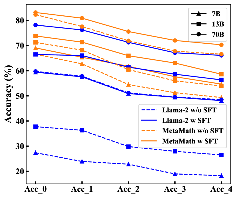
Figure 4: $\text{Acc}_{i}$ of LLaMA-2 and MetaMath families. "w" and "w/o" stand for "with" and "without" respectively.

There is a noticeable trend of diminishing accuracy from one round to the next for open-source LLMs, both prior to and after SFT, and the rate of accuracy decline from round to round is mitigated post-SFT, as illustrated in Figure 4. Our focus encompasses the LLaMA-2 family for general pre-trained LLMs and MetaMath for specialized LLMs, with model sizes spanning 7B, 13B, to 70B. This trend highlights the increased difficulty in solving longer questions, a challenge that mirrors the human experience, and incorporating extension as an auxiliary task can mitigate this effect. Interestingly, the accuracy of post-SFT LLaMA-2 can be comparable topre-SFT MetaMath, despite the fact that our $\mathcal{D}$ consists of only around 65K CoT data compared to 400K that MetaMath has been trained on. This observation suggests that extending the questions included in the training set could serve as an effective data augmentation strategy to improve the mathematical reasoning abilities of LLMs.

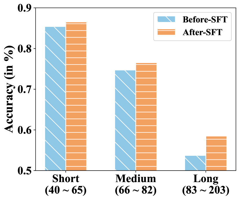
Figure 5: Accuracy on GSM8K with short, medium, and long length. The range of tokens within each category is in parenthesis.

Extension as an auxiliary task can further improve MetaMath [25] in solving longer questions on GSM8K. While MetaMath outperforms other math-related LLMs on GSM8K, it still faces challenges with lengthy MWPs [25]. To investigate whether extension would help, the GSM8K test set is divided into three subsets of equal size based on question length and the accuracy is calculated over each subset. As shown in Figure 5, extension not only benefits questions in all subsets but also yields the most significant performance improvement within long length group. Scaling up augmented data of extension by adding more rounds of extension to the training set (i.e., getting $\mathcal{D}_{r}$ for larger $r$) can be beneficial for LLMs to solve long MWPs as well. Some preliminary results regarding scaling up extension data are given in Appendix C.4. In addition, We believe applying other data augmentation methods provided by [25] to extended questions could be another way to mitigate the challenge of longer MWPs. We leave these for future work.

4.3 Generalization to Other Benchmarks

To evaluate generalizability, we assess CoRe and fine-tuned LLMs (without further SFT) on other benchmarks including MAWPS [10], SVAMP [11], and GSM-IC [12]. Detailed experimental setups are given in Appendix B.6. The results are shown in Table 5.

Both our CoRe and extension lead to superior performance across all evaluated benchmarks. These benchmarks consist of MWPs with concise descriptions, making the findings particularly notable: Despite being specifically tailored for long MWPs, these approaches are also effective for shorter MWPs. Remarkably, CoRe results in a $4.5\%$ absolute increase in accuracy on MAWPS with 0-CoT and $4.15\%$ on GSM-IC with PS+. Additionally, without further finetuning on the corresponding training set, our models (SFT on $\mathcal{D}$) yield an average accuracy increase of $15.28\%$ across different model sizes and benchmarks. This demonstrates the generalizability of our approaches in enhancing the performance of LLMs on MWPs.

	GPT-3.5-turbo				LLaMA-2
Dataset	CoRe	PS	PS+	0-CoT	SFT	7B	13B	70B
MAWPS	2717	90.77	91.78	91.40	2717	67.93	73.41	77.50
	1F5F8	91.57	93.38	92.67	1F5F8	72.52	78.21	87.74
SVAMP	2717	71.90	75.70	71.80	2717	50.50	61.70	73.30
	1F5F8	73.20	77.80	76.30	1F5F8	64.90	74.00	83.80
GSM-IC	2717	85.38	87.48	88.35	2717	33.55	48.45	65.70
	1F5F8	85.90	91.63	90.05	1F5F8	66.48	76.68	85.22

Table 5: Solving accuracy (in %) of proprietary and open-source LLMs on other MWP benchmarks.

5 Related Work

Prompting for Mathematical Reasoning. Mathematical reasoning [1, 6, 30] is recognized as a system-2 task [31, 32], attracting significant attention in the research community. Recent LLM advancements [2, 4, 33, 5] have led to diverse prompting strategies designed to enhance their ability to perform mathematical reasoning [34]. Notable among these is the Chain-of-Thought (CoT) prompting [8], which has significantly improved reasoning capabilities by encouraging the model to generate intermediate steps. While various few-shot techniques such as Re-reading [35] and Stepback prompting [36] have been developed, there is a growing interest in methodologies that enable zero-shot reasoning. These methods, such as the two-stage CoT prompting by [27], Plan-and-Solve (PS) prompting [28], and the self-discovery framework by [37], aim to equip LLMs to handle mathematical problems without few-shot demonstrations.

CoT Extension. Extensions to CoT encompass demonstration selection [38, 39, 40], advancements in decoding [29, 41], and developments for more intricate tasks [42, 43, 44, 45]. Further explorations within this domain have probed areas such as incorrect answer detection [46], investigations of failure modes [47, 12, 48, 49], and application in other math-related topics [50, 51, 52]. Our work pioneers the investigation of LLMs’ CoLeG in mathematical reasoning, employing a zero-shot prompting to isolate the influence of few-shot examplars.

Specialized LLMs for Mathematics. Despite general-purpose LLMs, there remains a persistent interest in maximizing the performace of domain-specific LLMs like mathematics, through strategies such as SFT and continued pretraining. Supervised fine-tuning methods, such as WizardMath’s [23] combination of PPO training and MAmmoTH’s [24] knowledge distillation of integrating CoT with Program-of-Thought[53, 54]. Additionally, MetaMath [25] rewrites mathematical questions in multiple formats to augment the training dataset. On the other hand, a distinct strand of research is dedicated to continuing pretraining of base LLMs on extensive mathematical corpora, exemplified by Minerva [55], Llemma [26], InternLM-MATH [56] and DeepSeekMath [57]. Our work explores to what extent CoLeG of these specialized mathematical LLMs will be improved by fine-tuning with our newly proposed auxiliary task - extension.

6 Conclusion

Our study explored LLMs’ ability to solve longer MWPs, i.e. CoLeG. We introduced a groundbreaking dataset, E-GSM, designed to test CoLeG of LLMs, along with two metrics to evaluate the efficacy and resilience of LLMs in this setting. Our investigation highlighted a notable CoLeG deficiency in existing zero-shot prompting techniques and open-source LLMs. A new instructional prompt, CoRe, and a new data augmentation technique, extension, not only significantly strengthened CoLeG but also show superior performance on GSM8K, and generalized well to other MWP benchmarks. By illuminating a previously underexplored aspect of LLMs’ reasoning and offering practical solutions to improve it, our work carved out new pathways for using LLMs in complex problem-solving and set the stage for future research on model generalizability and advanced SFT paradigms.

Limitations

Despite the innovative contributions of newly released E-GSM, CoRe, and the extension auxiliary task, our work still has some limitations. 1. Data Quality in E-GSM: Although heuristic methods are employed to control the quality of E-GSM, the dataset may still contain poorly constructed questions. Due to budget and time constraints, no complete human review of the dataset was performed. A more thorough human evaluation by well-funded institutions would be beneficial. 2. Generalizability Concerns: While the generalizability of our methods has been assessed using GSM-IC, our primary conclusions are derived from variants of the GSM8K dataset. Including additional benchmarks for MWPs would provide a more robust validation of our findings. However, conducting experiments on more datasets is resource-intensive. Therefore, we encourage further investigation by the research community. 3. Limited SFT Data: Owing to budget limitations, our released SFT data comprises approximately 65K examples. Further expansions could involve scaling up the extension augmented data, either by increasing the rounds of extension or applying other data augmented techniques. The exploration of alternative methods to extend SFT data and examining scalability effects also offers interesting avenues for future research. 4. Interpretability and Explainability: Even with the improved performance achieved by our methods, LLMs remain "black boxes." Understanding the intricate reasoning processes behind their solutions continues to be a significant challenge.

Broader Impacts

Our release of E-GSM presents a challenging benchmark to test the ability of LLMs to solve long MWPs. This aids future research by highlighting the intricacies involved in extended MWPs. Our innovative prompting method and the SFT technique have improved LLMs performance in these problems, potentially enhancing their generalization capabilities for real-world applications. This advancement not only broadens LLMs’ mathematical reasoning capacities, but also has implications for educational tools. However, despite progress, significant challenges in solving extended MWPs remain, calling for future refinements. Additionally, there is a risk of overreliance which might impede the development of critical thinking skill and problem-solving skills for human learners. Therefore, we point out the need for balanced use of LLM technologies, combining their benefits with critical human oversight.

Appendix A E-GSM Details

A.1 Examples in E-GSM

In E-GSM dataset, we extend original set of problems from GSM8K to longer ones round-by-round. GSM8K [6] is a benchmark of grade-school math word problems, containing a training set of 7473 examples, and a test set of 1319 problems. It is under MIT License and can be accessible at https://github.com/openai/grade-school-math. In table 6 , we show one particular original problem in GSM8K and its corresponding extension problems in the first two rounds. In total, our E-GSM consists of around 4.5K MWPs with extensive naratives, divided into four rounds (Table 1). E-GSM will be released under MIT License for future research.

$Q_{0}$

A mother goes shopping. She buys cocoa at $4.20, laundry at $9.45 and a package of pasta at $1.35. She pays $20. How much change does the cashier give back?

$Q_{1}$

On a bright Saturday morning, a mother decided to take advantage of the weekend sales at her local supermarket. With a shopping list in hand, she navigated through the aisles, picking up items she needed for the week. Among her finds were a rich, dark cocoa powder priced at $4.20, essential for her famous chocolate cake. Next, she grabbed a bottle of laundry detergent, a necessity for the upcoming week’s laundry, priced at $9.45. Lastly, she couldn’t resist adding a package of pasta to her cart, a steal at just $1.35, perfect for Wednesday night’s dinner. After browsing through the aisles and picking up a few more items, she made her way to the cashier. Handing over a crisp $20 bill to pay for her purchases, she waited for her change. How much change did the cashier hand back to her after her purchases?

$Q_{2}$

On a bright and sunny Saturday morning, the local supermarket was bustling with shoppers eager to take advantage of the weekend sales. Among them was a mother, who had meticulously prepared a shopping list to ensure she got everything needed for the upcoming week. As she entered the supermarket, her eyes scanned the aisles for the items on her list. Her first find was a rich, dark cocoa powder, priced at $4.20, essential for baking her famous chocolate cake that her family adored. Next, she picked up a bottle of laundry detergent, priced at $9.45, a necessity for tackling the week’s laundry pile. Lastly, she spotted a package of pasta, priced at just $1.35, perfect for the family’s Wednesday night dinner. With her cart filled with these items and a few more essentials, she confidently made her way to the cashier. After unloading her cart and watching the cashier scan each item, she handed over a crisp $20 bill to cover the cost of her purchases. As the cashier processed the transaction, she anticipated the change she would receive, knowing it would be just enough for a small treat for her children on the way home. How much change did the cashier hand back to her after her purchases?

Table 6: Examples from E-GSM.

A.2 Human Evaluation of E-GSM

To ensure the quality of E-GSM, we carried out a human evaluation on 50 selected seed questions and their corresponding extension questions in each round. Three annotators are asked to answer the following questions (Yes/No):

1. Does the order of the question descriptions (i.e., the conditions) remain the same after extension?

2. Are the conditions clear and unambiguous after extension?

3. Is the question solvable after extension (i.e., can an answer be derived from the conditions)?

4. Does the ground-truth answer remain the same after extension?

Then we can categorized these questions into three quality levels according to the answers of the previous questions: excellent, good, and poor.

• Excellent. Affirmative responses to all questions.

• Good. At least three affirmative responses, including a mandatory "Yes" to Question 3 and Question 4.

• Poor. Otherwise.

In Appendix A.1, we have shown an example at an excellent quality level. We show two examples of good and poor quality levels in table 7.

An Example Under Good Level

Original: John takes care of 10 dogs. Each dog takes .5 hours a day to walk and take care of their business. How many hours a week does he spend taking care of dogs?

Round-4: In a picturesque neighborhood, where the gentle whispers of nature blend harmoniously with the serene ambiance, lives a man named John. His love for dogs is not just a hobby but a profound passion that has transformed his spacious backyard into a haven for 10 lively dogs. Each dog, with its unique personality and zest for life, thrives under John’s care, enjoying the lush, green expanse as their playground. John, whose heart is as expansive as the open spaces he provides, starts his day with the first light of dawn, ready to embark on a journey of love and dedication with his canine family. John’s daily routine is a testament to his unwavering commitment to the well-being of his dogs. He takes each of his 10 dogs on a half-hour walk, exploring the scenic trails that meander through their neighborhood. These walks are more than just exercise; they are adventures filled with exploration, play, and moments of joy, allowing each dog to connect with the essence of nature. For John, these moments are sacred, an opportunity to deepen the bond with his dogs, ensuring their happiness and well-being are always at the forefront. Given John’s dedication to providing a fulfilling life for his dogs, how many hours does he devote each week to walking and caring for his beloved companions, ensuring they experience the joy, health, and exercise they deserve?

An Example Under Poor Level

Original: Andy’s car fuel efficiency is 10 MPG (miles per gallon). If the current price for regular gas is $3/gallon, how much money is Andy’s car consuming per week if he only uses his car to go to work from Monday to Friday and the one-way distance between his home and office is 5 miles?

Round-1: Andy, a dedicated employee at a bustling downtown firm, has a daily routine that involves driving his reliable car to work. His car, known for its decent fuel efficiency of 10 miles per gallon (MPG), is his chosen mode of transportation for the 5-mile journey from his cozy suburban home to the high-rise office building where he works. As the week begins on Monday, Andy prepares for his usual commute, aware that the current price for regular gasoline stands at $3 per gallon. Throughout the week, from Monday to Friday, Andy uses his car exclusively for his work commute, making the round trip each day with the intention of maximizing his time and efficiency. Given these circumstances, how much money is Andy’s car consuming per week for his work-related travels?

Table 7: Examples of extended problems of different quality. The example in good quality changes the original condition "Each dog takes .5 hours a day to walk and take care of their business" to "He takes each of his 10 dogs on a half-hour walk." The new condition does not include the time of "taking care of their business". The answer to questions 2 is "No". The poor quality problem disregards the original condition that "he only uses his car to go to work." The answer to question 4 is "No". The changes in conditions are highlighted by red.

A.3 Heuristic for Quality Control

To minimize human labor, we adopt a heuristic approach powered by an entailment model to automatically eliminate undesired examples after extension. Specifically, a score $S_{r}^{i}=ENT(q_{r}^{i},q_{0}^{i})$ is calculated to evaluate the informational equivalence between the extended and its corresponding seed questions.

For this purpose, we utilize the SAUMMAC zero-shot model [18], an entailment model trained on MNLI [58]. This model represents a consistency detection technique in text summarization, employing an off-the-shelf natural language inference model to determine the pairwise entailment score between texts. To detect all potential informational mismatches in any sentence, we aggregate sentence-level entailment with the $min$ operation:

$$ENT(q_{r}^{i},q_{0}^{i})=\min_{j}\max_{k}ent(a_{k},b_{j}),$$

where $a_{k},b_{j}$ are sentences of $q_{r}^{i},q_{0}^{i}$ respectively, $ent$ represents the probability of entailment, the $min$ is taken over all sentences of $q_{0}^{i}$, and $max$ is taken over all sentences of $q_{r}^{i}$. A small $S_{r}^{i}$ can suggest a potentially unsatisfactory extension, leading to the exclusion of the question $q_{r}^{i}$ if $S_{r}^{j}<0.2,\text{for any}j\leq r$. Ultimately, human evaluation (see Appendix A.2) has shown that this approach effectively filters out all unsatisfactory questions.

Appendix B Experimental Setup

B.1 LLMs

A variety of proprietary LLMs used in our study of zero-shot prompting methods are listed below:

• GPT-3.5-turbo-instruct: This model showcases capabilities akin to those of text-davinci-003, ensuring compatibility with the legacy Completions endpoint.

• GPT-3.5-turbo: This represents a refined version within the GPT-3.5 series, equipped with an enhanced understanding and generation of both natural language and coding content. We employed the gpt-3.5-turbo-0125 engine for our experiments.

• GPT-4-turbo: Considered as the forefront of the GPT series, we utilized the gpt-4-0125-preview engine in our work.

• Gemini-Pro: Developed by Google, this model is touted for its unmatched scalability across a broad spectrum of tasks. Further information about the API is available at https://cloud.google.com/vertex-ai/docs/generative-ai/model-reference/gemini.

• Claude-3: This model is released by Anthropic recently, which is claimed to be comparable or even surpass GPT-4. We use Claude-3-opus-20240229 and Claude-3-sonnet-20240229 engines.

• GLM-3 [19]: The details of these models can be found in https://github.com/THUDM/ChatGLM3/blob/main/README_en.md. We use glm-3-turbo engine.

Access to all OpenAI APIs can be found at https://platform.openai.com/docs/models/overview. Furthermore, the creation of our new E-GSM dataset (Section 2.2) utilizes GPT-4-turbo. To acquire SFT data, GPT-3.5-turbo is leveraged to generate CoT chains (Section 3.3). GPT-3.5-turbo is also instrumental in extracting answers from the responses generated by various LLMs (Section B.3).

To explore SFT, our study employs an array of open-source LLMs and specialized mathematical LLMs.

• LLaMA-2 families: We engage with models of varying scales—7B, 13B, and 70B—specifically leveraging the instruction-tuned versions. The instruction-tuned LLaMA-2 is accessible at https://huggingface.co/meta-llama/Llama-2-70b-chat-hf. They are under Llama2 License.

• Mistral-7B: The model has undergone instruction-tuning and is available at https://huggingface.co/mistralai/Mistral-7B-Instruct-v0.2. It is under Apache License 2.0.

• WizardMath [23]: This family of models enhances the mathematical reasoning abilities of both LLaMA-2 and Mistral-7B through reinforcement learning. The models can be found at https://huggingface.co/WizardLM. They follow the same license as LLaMA-2 (see https://github.com/nlpxucan/WizardLM/tree/main/WizardMath).

• MAmmoTH [24]: A family of models that has been instruction-tuned on a CoT and program-of-thought with Llama-2 families and Mistral-7B. They are available ahttps://huggingface.co/TIGER-Lab. They follow the license.

• MetaMath [25]: This approach fine-tunes LLaMA-2 and Mistral-7B on MetaMathQA, a dataset augmented by rewriting original training questions from multiple perspectives. We also incorporate MetaMath-Llemma. All models are available at https://huggingface.co/meta-math. The license for each model can be found at https://github.com/meta-math/MetaMath?tab=readme-ov-file.

• Llemma [26]: Representing open-source LLMs for mathematics, Llemma is continually pre-trained using CodeLLaMA on Proof-Pile-2. In our experiments, we use the Llemma-7B model, which is available at https://huggingface.co/EleutherAI/llemma_7b. It is under Apache License 2.0.

• DeepSeekMath-7B [57]: Specialized mathematical models that have undergone further pre-training on math-related tokens. We use the deepseek-math-7b-instruct model, which is available at https://huggingface.co/deepseek-ai/deepseek-math-7b-instruct. The license can be found at https://github.com/deepseek-ai/DeepSeek-Math/blob/main/LICENSE-MODEL.

• LLaMA-3 families: We also include LLaMA-3 families released most recently, including 8B and 70B models. The models are accessible at https://huggingface.co/collections/meta-llama/meta-llama-3-66214712577ca38149ebb2b6. They are under Llama3 License.

B.2 SFT Data Examples

Our entire training set includes 64,929 CoT data, with 38,507 from the original CoT augmented training set $\mathcal{D}_{0}$ and 26,422 CoT data for extended questions $\mathcal{D}_{1}$. Following [25], we use the training prompt in Table 9, where the instruction is replaced by training example from $\mathcal{D}_{0}$ or $\mathcal{D}_{1}$. For scaling up extended questions, there are 24,147 training examples in $\mathcal{D}_{2}$ (see Section 4.2 and Appendix C.4). We showcase one concrete example from $\mathcal{D}_{0}$, $\mathcal{D}_{1}$, and $\mathcal{D}_{2}$ in Table 10 and one can find more examples in our released SFT dataset $\mathcal{D}$. $\mathcal{D}$ includes a total of approximately 89K CoT data, covering all examples within $\mathcal{D}_{0},\mathcal{D}_{1},\mathcal{D}_{2}$. This dataset will be made available under MIT License. Note that $\mathcal{D}_{2}$ is only used in Figure 7 and Appendix C.4.

Below is an instruction that describes a task. Write a response that appropriately completes the request.

### Instruction:

{instruction}

### Response:

Table 8: Training prompt for Open-source LLMs.

Below is an instruction that describes a task. Write a response that appropriately completes the request.

### Instruction:

{instruction}

### Response: Let’s think step by step

Table 9: Evaluation prompt for Open-source LLMs.

An example from $D_{0}$

Instruction: Natalia sold clips to 48 of her friends in April, and then she sold half as many clips in May. How many clips did Natalia sell altogether in April and May?

Response: Natalia sold 48 clips in April. In May, she sold half as many, which is 48 / 2 = 24 clips. Altogether, she sold 48 + 24 = 72 clips in April and May.

An example from $D_{1}$

Instruction: In the bustling town of Willow Creek, Natalia had become quite the entrepreneur with her homemade clip business. In the month of April, her creativity and hard work paid off when she managed to sell her beautifully crafted clips to 48 of her friends, each one more eager than the last to support her venture. As the flowers began to bloom and May rolled around, Natalia continued her efforts, though she found that the demand had slightly decreased. By the end of May, she realized she had sold exactly half the number of clips she did in April. With these two months of sales combined, how many clips did Natalia sell altogether in April and May?

Response: In April, Natalia sold 48 clips. In May, she sold half of the number she sold in April, which is 48/2 = 24 clips. Therefore, Natalia sold 48 + 24 = 72 clips altogether in April and May.

An example from $D_{2}$

Instruction: In the charming town of Willow Creek, nestled among rolling hills and vibrant flower fields, Natalia had carved out a niche for herself as a budding entrepreneur with a unique talent for crafting homemade clips. Her designs, infused with creativity and a personal touch, quickly caught the eye of her friends and neighbors. In the blossoming month of April, as the community came alive with the sights and sounds of spring, Natalia’s business flourished. She found herself busily fulfilling orders for 48 of her friends, each one more enthusiastic than the last to support her burgeoning venture and adorn their outfits with her unique creations. As the calendar turned to May, the fresh blooms of April gave way to the full splendor of spring. Natalia, ever dedicated to her craft, continued to pour her heart and soul into each clip she made. However, she noticed a slight shift in the air. The initial surge of excitement that had greeted her April launch had tempered somewhat, and the pace of orders had slowed. By the time the final days of May had drawn to a close, Natalia took stock of her efforts and realized that the number of clips she had sold this month was exactly half of what she had managed in April. Reflecting on these two months of hard work and the support of her community, Natalia wondered: How many clips had she sold altogether in April and May, marking the beginning of her journey as an entrepreneur in Willow Creek?

Response: In April, Natalia sold 48 clips to her friends. In May, she sold half of what she sold in April, which means she sold 48 / 2 = 24 clips in May. To find out how many clips she sold altogether in April and May, we add the number of clips sold in April and May: 48 (April) + 24 (May) = 72 clips. Therefore, Natalia sold 72 clips altogether in April and May, marking the beginning of her journey as an entrepreneur in Willow Creek.

Table 10: Training Examples.

B.3 Answer Extraction

Unlike previous works [23, 25] that derive the final answer by extracting strings following the phrase "The answer is", we use GPT-3.5-turbo fo answer extraction as given in Table 11. This strategy is adept at handling atypical cases that cannot be readily resolved using trigger words like "The answer is", which appears with various LLMs each presenting distinct output formats in zero-shot manner. Preliminary extraction has shown that over $99.8\%$ of responses have been accurately extracted. Following [25], for the SFT data mentioned in Section B.4, we append "The answer is" to the answers extracted from GPT-3.5-turbo at the end of responses. Nevertheless, to ensure fairness, we also employ our innovative answer extraction technique for our fine-tuned LLMs.

Given the last ’Quesion’ and ’Answer’, your goal is to extract the final numerical result from the ’Answer’ part, and put the numerical result after the ’Result’ part. You must not to solve the problem by yourself, all you need to do is give me just a number extracted from ’Answer’.

Table 11: Prompt for answer extraction.

B.4 SFT Details

In our experiments with the LLaMA-2 backbone, the learning rates are chosen based on the model scale. For LLMs with parameters of 7B and 13B, the learning rate is set to $0.00002$. For 70B LLMs, the learning rate is adjusted to $0.00001$. For the Mistral-7B base model, the learning rate is further reduced to $0.000005$ to maintain the stability of the training. The learning rate is set to $0.00002$ for LLaMA-3-8B and $0.00001$ for LLaMA-3-70B.

Batch sizes are also tailored to LLMs parameters to maximize the utilization of computational resources. Specifically, for the 70B model, we select a batch size of 24 per device. For models with 7B and 13B parameters, a larger batch size of 36 per device is chosen.

All models undergo training for 3 epochs with AdamW optimizer with a $3\%$ learning rate warmup. Experiments for LLMs with sizes 7B and 13B are conducted on 4 $\times$ H800 GPUs. For the larger 70B model, necessitating more computational power, the experiments are carried out on 8 $\times$ H800 GPUs (80G). The most computation-expensive experiment (fine-tune a 70B model) takes around $190$ GPU hours. The entire experiment takes around 1,600 GPU hours (excluding preliminary or failed experiments).

During inference, we apply greedy decoding with a temperature of $0.0$ and the maximum generation length is set to $512$. Following [25], we use the zero-shot evaluation prompting, as shown in Table 9, where the instruction is replaced by the testing question.

All our SFT models will be made available for reproduction and future research endeavors. The license for these models will adhere to the same license applicable to the models prior to fine-tuning.

B.5 Contrast Coefficients

$C=[C_{1},C_{2},...,C_{k-1}]$ is the contrast coefficients, where each $C_{i}$ is assigned based on the hypothesized trend. The contrast $C$ is used to test the significance of the hypothesized trend across levels of $\beta$. In our case, the contrast coefficients that we use are centered linear trend coefficients. For example, $[-2.-1,0,1,2]$ is used for $[C_{1}.C_{2},...,C_{5}]$. Note that the absolute difference $C_{i}-C_{i-1}$ does not matter because we want to test $C\cdot\beta=0$ and we can divide both sides by any number except 0.

B.6 Generalizability Setup

Here we give a brief introduction to the benchmark datasets we used in Section 4.3.

• MAWPS [10] is a benchmark of MWPs, incorporating 238 test examples. It is under MIT License and can be found at https://github.com/LYH-YF/MWPToolkit.

• SVAMP [11] includes 1,000 simple MWPs, which is available at https://github.com/LYH-YF/MWPToolkit. It is under MIT License.

• GSM-IC [12] is a variant of GSM8K, including MWPs with one irrelevant sentence. The dataset is available at https://github.com/google-research-datasets/GSM-IC. Following [12], we randomly sampled 4K questions as our test set for evaluation.

Appendix C Further Results

C.1 Training Curves

Figure 6 depicts the CoLeG-E and CoLeG-R for both LLaMA-2-7B and Mistral-7B throughout 1,200 fine-tuning steps, equivalent to three complete epochs. Initially, the performance of both models improves rapidly before stabilizing at a later stage. This trend underscores the effectiveness of SFT in improving CoLeG.

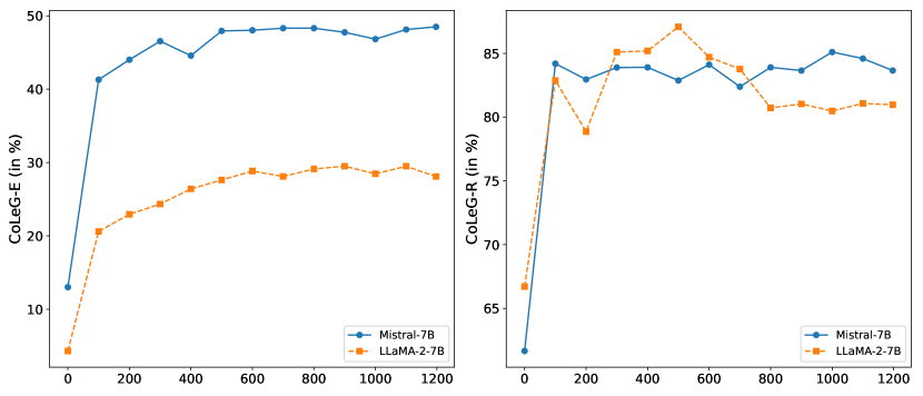
Figure 6: The performance curves of LLaMA-2-7B and Mistral-7B during 1,200 fine-tuning steps. Left: CoLeG-E; Right: CoLeG-R. The x-axis is the training steps during fine-tuning.

C.2 Complete Results of Prompting Methods

We have provided some representative results of prompting methods in Table 2 in Section 4.1. Here we release complete and detailed prompting results of 7 proprietary LLMs and 3 prompting methods in Table 14 and 15. It can be observed that our Condition-Retrieving Instruction achieves notable performance improvement for LLMs with weaker proficiency, yet shows nuanced enhancement for strong LLMs such as GPT-4 and Claude-3-Haiku. This phenomenon suggests that proficient LLMs may encounter greater challenges when addressing reasoning difficulties arising from long context math problems than precisely extracting conditions from original problem.

C.3 Complete Results of SFT

Section 4.2 presents the main results of SFT on $\mathcal{D}$. The exhaustive results are detailed in Table 12 and 13, including 18 LLMs of various scales and base models. From the results, it is clear that SFT significantly enhances both CoLeG-E and CoLeG-R in all open-source and math-specific LLMs examined. Interestingly, the performance of LLaMA-2 with SFT on the $\mathcal{D}$ achieves levels comparable to those of specialized mathematical LLMs. It is important to note that our SFT dataset $\mathcal{D}$ only consists of approximately 65K entries, whereas MetaMath [25] incorporates around 400K CoT data. This suggests that extending problems in the training set might be another auxiliary task for mathematical reasoning.

Model	CoLeG-E	CoLeG-R	$\text{Acc}_{0}$	$\text{Acc}_{1}$	$\text{Acc}_{2}$	$\text{Acc}_{3}$	$\text{Acc}_{4}$
LLaMA-2-7B Models
LLaMA-2-7B	4.31	66.71	27.37	23.93	22.83	18.97	18.26
+ SFT on $\mathcal{D}$	28.09	80.97	59.44	57.57	50.92	49.46	48.13
	(+23.78)	(+14.26)	(+32.07)	(+33.64)	(+28.09)	(+30.49)	(+29.87)
MAmmoTH-7B	11.52	66.09	47.46	45.02	34.91	32.67	31.37
+ SFT on $\mathcal{D}$	30.15	80.25	62.77	60.00	54.42	52.18	50.37
	(+18.63)	(+14.16)	(+15.31)	(+14.98)	(+19.51)	(+19.51)	(+19.00)
WizardMath-7B	11.89	59.72	52.99	43.77	38.41	33.58	31.65
+ SFT on $\mathcal{D}$	31.37	76.77	63.91	58.83	58.09	52.45	49.06
	(+19.48)	(+17.05)	(+10.92)	(+15.06)	(+19.68)	(+18.87)	(+17.41)
MetaMath-7B	31.74	74.13	66.57	62.76	54.51	51.27	49.34
+ SFT on $\mathcal{D}$	38.01	79.17	69.07	65.36	61.77	57.62	54.68
	(+6.27)	(+5.04)	(+2.50)	(+2.60)	(+7.26)	(+6.35)	(+5.34)
Mistral-7B Models
Mistral-7B	13.01	61.66	50.57	45.27	39.55	37.30	31.18
+ SFT on $\mathcal{D}$	48.50	83.65	76.12	74.48	69.82	66.70	63.67
	(+35.49)	(+21.99)	(+25.55)	(+29.21)	(+30.27)	(+29.40)	(+32.49)
WizardMath-Mistral-7B	50.94	79.13	82.71	76.90	70.78	68.78	65.45
+ SFT on $\mathcal{D}$	52.81	82.72	81.96	80.33	74.28	71.87	67.79
	(+1.87)	(+3.59)	(-0.75)	(+3.43)	(+3.50)	(+3.09)	(+2.34)
MetaMath-Mistral-7B	43.63	75.69	77.56	72.80	66.75	60.89	58.71
+ SFT on $\mathcal{D}$	49.72	82.33	78.24	77.32	71.13	68.78	64.42
	(+6.09)	(+6.64)	(+0.68)	(+4.52)	(+4.38)	(+7.89)	(+5.71)
Other 7B Models
llemma_7b	2.06	66.63	28.81	27.64	23.10	20.05	19.19
+ SFT on $\mathcal{D}$	33.05	80.71	67.17	62.59	58.09	54.54	54.21
	(+30.99)	(+14.08)	(+38.36)	(+34.95)	(+34.99)	(+34.49)	(+35.02)
deepseek-math-7b	42.98	69.07	81.88	76.57	66.67	62.79	56.55
+ SFT on $\mathcal{D}$	51.31	80.34	81.35	77.91	72.35	67.88	65.36
	(+8.33)	(+11.27)	(-0.53)	(+1.34)	(+5.68)	(+5.09)	(+8.81)
MetaMath-Llemma-7B	28.18	64.77	68.23	62.34	53.81	49.55	44.19
+ SFT on $\mathcal{D}$	38.86	77.32	70.96	67.78	62.73	57.62	54.87
	(+10.68)	(+12.55)	(+2.73)	(+5.44)	(+8.92)	(+8.07)	(+10.68)
LLaMA-2-13B Models
LLaMA-2-13B	8.61	70.18	37.76	36.32	29.83	27.95	26.50
+ SFT on $\mathcal{D}$	37.27	84.78	66.49	66.03	61.42	58.62	56.37
	(+28.66)	(+14.60)	(+28.73)	(+29.71)	(+31.59)	(+30.67)	(+29.87)
MAmmoTH-13B	18.63	74.07	55.12	52.97	45.76	45.01	40.82
+ SFT on $\mathcal{D}$	42.32	85.54	71.04	69.12	65.62	62.25	60.77
	(+23.69)	(+11.47)	(+15.92)	(+16.15)	(+19.86)	(+17.24)	(+19.95)
WizardMath-13B	19.29	72.12	57.77	54.90	45.49	42.29	41.67
+ SFT on $\mathcal{D}$	41.76	84.29	71.65	69.71	63.87	59.98	60.39
	(+22.47)	(+12.17)	(+13.88)	(+14.81)	(+18.38)	(+17.69)	(+18.72)
MetaMath-13B	36.14	75.68	71.27	68.20	60.45	55.99	53.93
+ SFT on $\mathcal{D}$	44.10	79.38	73.84	71.38	65.97	63.07	58.61
	(+7.96)	(+3.70)	(+2.57)	(+3.18)	(+5.52)	(+7.08)	(+4.68)

Table 12: Complete results of the effect of SFT on CoLeG. All figures are in $\%$, and the SFT results are shaded. Differences between SFT results and original ones are shown in parentheses.

Model	CoLeG-E	CoLeG-R	$\text{Acc}_{0}$	$\text{Acc}_{1}$	$\text{Acc}_{2}$	$\text{Acc}_{3}$	$\text{Acc}_{4}$
LLaMA-2-70B Models
LLaMA-2-70B	26.50	81.19	59.74	57.82	51.18	49.55	48.50
+ SFT on $\mathcal{D}$	49.81	84.57	78.17	76.23	71.30	67.15	66.10
	(+23.31)	(+3.38)	(+18.43)	(+18.41)	(+20.12)	(+17.60)	(+17.60)
WizardMath-70B	45.97	78.75	80.14	76.49	69.29	65.34	63.11
+ SFT on $\mathcal{D}$	54.68	82.60	82.41	80.59	74.89	71.87	68.07
	(+8.71)	(+3.85)	(+2.27)	(+4.10)	(+5.60)	(+6.53)	(+4.96)
MAmmoTH-70B	42.98	85.24	72.93	74.48	69.20	64.52	62.17
+ SFT on $\mathcal{D}$	55.15	83.25	81.88	80.67	74.37	71.05	68.16
	(+12.17)	(-1.99)	(+8.95)	(+6.19)	(+5.17)	(+6.53)	(+5.99)
MetaMath-70B	52.81	80.86	82.34	77.57	71.92	67.79	66.57
+ SFT on $\mathcal{D}$	57.12	84.55	83.17	80.92	75.59	72.05	70.32
	(+4.31)	(+3.69)	(+0.83)	(+3.35)	(+3.67)	(+4.26)	(+3.75)
LLaMA-3 Models
Meta-Llama-3-8B	8.24	76.14	41.32	43.68	37.13	33.94	31.46
+ SFT on $\mathcal{D}$	47.57	84.82	75.28	74.23	69.47	67.88	63.86
	(+39.33)	(+8.68)	(+33.96)	(+30.55)	(+32.34)	(+33.94)	(+32.40)
Meta-Llama-3-70B	40.71	85.56	72.91	71.38	67.98	66.79	62.38
+ SFT on $\mathcal{D}$	64.70	83.96	88.55	86.36	80.14	76.77	74.34
	(+23.99)	(-1.60)	(+15.64)	(+14.98)	(+12.16)	(+9.98)	(+11.96)

Table 13: Complete results of the effect of SFT on CoLeG. All figures are in $\%$, and the SFT results are shaded. Differences between SFT results and original ones are shown in parentheses. (Con’t)

C.4 Scaling up SFT Data

During the construction of the E-GSM (refer to Section 2.2), we use a round-by-round extension strategy, which can also be applied to augment the original GSM8K training set. The primary findings utilize $\mathcal{D}=\mathcal{D}_{0}\cup\mathcal{D}_{1}$ for SFT, and we can study the effect of enlarging SFT dataset through this specific extension strategy based on $\mathcal{D}_{1}$. Consequently, we examine the effects of SFT on CoLeG in four distinct scenarios: without SFT, SFT on $\mathcal{D}_{0}$, SFT on $\mathcal{D}_{0},\mathcal{D}_{1}$, SFT on $\mathcal{D}_{0},\mathcal{D}_{1},\mathcal{D}_{2}$. Figure  have shown the performance in different settings, and the additional outcomes are presented in Figure 7 and 8.

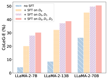
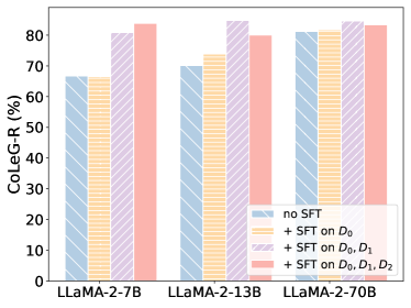
Figure 7: CoLeG-E (left) and CoLeG-R (right) of scaling up SFT dataset across various model scales in the LLaMA-2 family. The results suggest scaling up model scales and SFT dataset can further improve CoLeG.

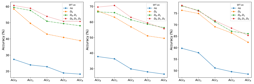
Figure 8: The changes in $\text{Acc}_{i}$ when LLMs are fine-tuned on different SFT dataset. Left: LLaMA-2-7B; Middle: LLaMA-2-13B; right: LLaMA-2-70B.

Prompting Techniques	CoLeG-E	CoLeG-R	$\text{Acc}_{0}$	$\text{Acc}_{1}$	$\text{Acc}_{2}$	$\text{Acc}_{3}$	$\text{Acc}_{4}$
Claude-3-haiku
Plan-and-Solve	62.27	84.90	88.78	84.94	78.74	77.40	75.37
+ CoRe	62.64	83.55	89.54	85.36	78.74	78.49	74.81
	(+0.37)	(-1.35)	(+0.76)	(+0.42)	(+0.00)	(+1.09)	(-0.56)
Plan-and-Solve+	62.64	82.58	90.14	86.19	81.10	78.58	74.44
+ CoRe	62.55	83.59	89.61	84.85	80.66	77.04	74.91
	(-0.09)	(+1.01)	(-0.53)	(-1.34)	(-0.44)	(-1.54)	(+0.47)
Zero-Shot CoT	62.83	83.07	89.61	85.52	80.05	77.13	74.44
+ CoRe	64.14	83.56	89.31	86.69	81.36	77.22	74.63
	(+1.31)	(+0.49)	(-0.30)	(+1.17)	(+1.31)	(+0.09)	(+0.19)
Claude-3-opus
Plan-and-Solve	74.81	84.07	95.45	92.30	88.28	85.30	80.24
+ CoRe	78.00	87.07	95.60	92.47	88.89	86.12	83.24
	(+3.18)	(+3.00)	(+0.15)	(+0.17)	(+0.61)	(+0.82)	(+3.00)
Plan-and-Solve+	75.00	84.79	95.30	91.38	87.49	84.48	80.81
+ CoRe	78.28	86.01	95.91	92.72	88.54	86.03	82.49
	(+3.28)	(+1.22)	(+0.61)	(+1.34)	(+1.05)	(+1.54)	(+1.69)
Zero-Shot CoT	74.72	86.08	94.09	91.80	87.58	84.57	80.99
+ CoRe	77.81	86.29	95.38	92.64	88.98	85.39	82.30
	(+3.09)	(+0.21)	(+1.29)	(+0.84)	(+1.40)	(+0.82)	(+1.31)
Gemini-pro
Plan-and-Solve	46.25	77.35	80.74	75.82	69.99	65.15	62.45
+ CoRe	47.10	79.48	80.82	76.57	71.48	65.34	64.23
	(+0.84)	(+2.13)	(+0.08)	(+0.75)	(+1.49)	(+0.18)	(+1.78)
Plan-and-Solve+	48.22	79.19	80.52	76.82	70.25	66.88	63.76
+ CoRe	49.91	81.99	80.74	78.33	71.57	66.88	66.20
	(+1.69)	(+2.79)	(+0.23)	(+1.51)	(+1.31)	(+0.00)	(+2.43)
Zero-Shot CoT	49.20	75.69	83.70	77.91	71.83	66.76	63.36
+ CoRe	53.65	81.44	83.70	81.26	75.48	72.78	68.16
	(+4.45)	(+5.75)	(+0.00)	(+3.35)	(+3.65)	(+6.02)	(+4.81)
GLM-3-turbo
Plan-and-Solve	42.03	75.58	81.79	74.79	71.30	65.76	61.82
+ CoRe	39.94	77.33	82.04	77.66	71.80	67.06	63.44
	(-2.08)	(+1.75)	(+0.25)	(+2.87)	(+0.50)	(+1.30)	(+1.62)
Plan-and-Solve+	44.09	80.66	81.41	75.21	71.37	68.40	65.67
+ CoRe	42.79	78.59	82.57	78.11	70.95	67.39	64.89
	(-1.30)	(-2.07)	(+1.16)	(+2.90)	(-0.42)	(-1.00)	(-0.78)
Zero-Shot CoT	43.82	77.85	82.63	76.61	71.68	67.52	64.33
+ CoRe	45.96	79.84	81.93	78.71	71.93	69.35	65.41
	(+2.14)	(+1.99)	(-0.70)	(+2.10)	(+0.25)	(+1.83)	(+1.09)

Table 14: Complete results of various proprietary LLMs with prompting methods on E-GSM.

Prompting Techniques	CoLeG-E	CoLeG-R	$\text{Acc}_{0}$	$\text{Acc}_{1}$	$\text{Acc}_{2}$	$\text{Acc}_{3}$	$\text{Acc}_{4}$
GPT-3.5-turbo
Plan-and-Solve	41.76	80.43	78.70	76.65	70.87	67.15	63.30
+ CoRe	42.98	81.86	79.38	78.24	71.39	67.60	64.98
	(+1.22)	(+1.43)	(+0.68)	(+1.59)	(+0.52)	(+0.45)	(+1.69)
Plan-and-Solve+	48.03	81.14	80.67	78.83	72.70	68.87	65.45
+ CoRe	50.09	81.12	81.96	78.58	73.49	71.05	66.48
	(+2.06)	(-0.02)	(+1.29)	(-0.25)	(+0.79)	(+2.18)	(+1.03)
Zero-Shot CoT	46.63	79.63	80.89	77.91	72.53	68.24	64.42
+ CoRe	51.97	83.64	83.40	81.26	75.33	73.23	69.76
	(+5.34)	(+4.01)	(+2.50)	(+3.35)	(+2.80)	(+4.99)	(+5.34)
GPT-3.5-turbo-instruct
Plan-and-Solve	25.75	70.15	70.20	63.43	55.73	52.36	49.25
+ CoRe	23.50	70.82	69.14	61.09	55.21	50.18	48.97
	(-2.25)	(+0.67)	(-1.06)	(-2.34)	(-0.52)	(-2.18)	(-0.28)
Plan-and-Solve+	31.18	72.48	72.86	64.18	58.27	55.54	52.81
+ CoRe	30.43	81.27	70.05	65.86	60.72	57.08	56.93
	(-0.75)	(+8.78)	(-2.81)	(+1.67)	(+2.45)	(+1.54)	(+4.12)
Zero-Shot CoT	31.84	71.90	74.75	69.79	61.33	57.71	53.75
+ CoRe	35.96	80.17	73.69	68.20	62.64	60.34	59.08
	(+4.12)	(+8.28)	(-1.06)	(-1.59)	(+1.31)	(+2.63)	(+5.34)
GPT-4
Plan-and-Solve	75.66	86.12	94.92	92.47	87.23	83.85	81.74
+ CoRe	75.47	84.29	95.53	92.55	86.96	84.21	80.52
	(-0.19)	(-1.82)	(+0.61)	(+0.08)	(-0.26)	(+0.36)	(-1.22)
Plan-and-Solve+	75.84	84.79	95.30	92.22	86.70	84.21	80.81
+ CoRe	76.03	85.19	95.07	92.72	88.36	84.12	80.99
	(+0.19)	(+0.40)	(-0.23)	(+0.50)	(+1.66)	(-0.09)	(+0.19)
Zero-Shot CoT	76.69	85.68	95.07	92.64	87.66	84.75	81.46
+ CoRe	77.53	85.40	95.83	93.05	87.58	84.30	81.84
	(+0.84)	(-0.29)	(+0.76)	(+0.42)	(-0.09)	(-0.45)	(+0.37)

Table 15: Complete results of various proprietary LLMs with prompting methods on E-GSM (Con’t).

Model	CoLeG-E	CoLeG-R	$\text{Acc}_{0}$	$\text{Acc}_{1}$	$\text{Acc}_{2}$	$\text{Acc}_{3}$	$\text{Acc}_{4}$
LLaMA-2-7B	4.31	66.71	27.37	23.93	22.83	18.97	18.26
+ SFT on $\mathcal{D}_{0}$	20.22 (+15.91)	66.64 (-0.07)	58.45 (+31.08)	49.62 (+25.69)	42.96 (+20.13)	40.93 (+22.96)	38.95 (+20.69)
+ SFT on $\mathcal{D}_{0},\mathcal{D}_{1}$	28.09 (+23.78)	80.97 (+14.26)	59.44 (+32.07)	57.57 (+33.64)	50.92 (+28.09)	49.46 (+30.49)	48.13 (+29.87)
+ SFT on $\mathcal{D}_{0},\mathcal{D}_{1},\mathcal{D}_{2}$	30.34 (+26.03)	83.83 (+17.12)	60.65 (+33.28)	58.91 (+35.98)	53.89 (+31.06)	50.91 (+32.14)	50.84 (+32.18)
LLaMA-2-13B	8.61	70.18	37.76	36.32	29.83	27.95	26.50
+ SFT on $\mathcal{D}_{0}$	32.40 (+23.79)	73.91 (+3.73)	67.02 (+29.26)	63.10 (+26.78)	56.87 (+27.04)	51.09 (+23.14)	49.53 (+23.03)
+ SFT on $\mathcal{D}_{0},\mathcal{D}_{1}$	37.27 (+28.66)	84.78 (+14.60)	66.49 (+28.73)	66.03 (+29.71)	61.42 (+31.59)	58.62 (+30.67)	56.37 (+29.87)
+ SFT on $\mathcal{D}_{0},\mathcal{D}_{1},\mathcal{D}_{2}$	38.86 (+30.25)	80.05 (+9.87)	69.60 (+31.84)	70.63 (+34.31)	62.99 (+33.16)	59.44 (+31.49)	55.71 (+29.21)
LLaMA-2-70B	26.50	81.19	59.74	57.82	51.18	49.55	48.50
+ SFT on $\mathcal{D}_{0}$	45.32 (+18.82)	81.76 (+0.57)	76.27 (+16.53)	74.90 (+17.08)	69.12 (+17.94)	66.42 (+16.87)	62.36 (+13.86)
+ SFT on $\mathcal{D}_{0},\mathcal{D}_{1}$	49.81 (+23.31)	84.57 (+3.38)	78.17 (+18.43)	76.23 (+18.41)	71.30 (+20.12)	67.15 (+17.60)	66.10 (+17.60)
+ SFT on $\mathcal{D}_{0},\mathcal{D}_{1},\mathcal{D}_{2}$	50.66 (+24.16)	83.37 (+2.18)	78.39 (+18.65)	75.98 (+18.16)	71.74 (+20.56)	68.51 (+18.96)	65.36 (+16.86)

Table 16: Complete results of the effect of scaling up SFT dataset on CoLeG. All figures are in $\%$. Differences between the SFT results and the original are shown in parentheses. The best results within each model scale are shown in bold. In general, scaling up SFT dataset can improve CoLeG.

Appendix D Prompts in Experiments

The 8-shot CoT experiment on GSM8K (see Section 2.1) with GPT-3.5-turbo (see Section B.1) uses prompts provided by [8]. The full prompt is given in Table 17.

For the construction of the E-GSM (see Section 2.2), we provide the template for extension in Figure 2. Table 18 shows the complete prompts for the first two rounds of extension, and all prompts will be released in our code repository.

Moreover, all zero-shot prompting including our proposed prompt methods along with their format are presented in Table 19. Our investigated zero-shot prompting including zero-shot CoT [27], Plan-and-Solve [28] and its variant PS+.

Zero-shot CoT [27], a variant of CoT [8], prompts the model directly with the problem of interest followed by "Let’s think step by step," without providing any demonstration examples.

Plan-and-Solve [28] enhances 0-CoT by initially prompting LLMs to create a plan that breaks down the overarching task into subtasks, subsequently executing these subtasks in accordance with the devised plan. Additionally, we investigate a variant of PS, identified as PS+, designed to mitigate calculation inaccuracies.

Here, since our prompt is typically prepended to other prompts, “ Other prompting method ” refers to the prompt words of various other prompting methods, like “Let’s think step by step” for 0-CoT.

Q: There are 15 trees in the grove. Grove workers will plant trees in the grove today. After they are done, there will be 21 trees. How many trees did the grove workers plant today?

A: There are 15 trees originally. Then there were 21 trees after the Grove workers planted some more. So there must have been 21 - 15 = 6 trees that were planted. The answer is 6.

Q: If there are 3 cars in the parking lot and 2 more cars arrive, how many cars are in the parking lot?

A: There are originally 3 cars. Then 2 more cars arrive. Now 3 + 2 = 5 cars are in the parking lot. The answer is 5.

Q: Leah had 32 chocolates and her sister had 42. If they ate 35, how many pieces do they have left in total?

A: Originally, Leah had 32 chocolates and her sister had 42. So in total they had 32 + 42 = 74. After eating 35, they had 74 - 35 = 39 pieces left in total. The answer is 39.

Q: Jason had 20 lollipops. He gave Denny some lollipops. Now Jason has 12 lollipops. How many lollipops did Jason give to Denny?

A: Jason had 20 lollipops originally. Then he had 12 after giving some to Denny. So he gave Denny 20 - 12 = 8 lollipops. The answer is 8.

Q: Shawn has five toys. For Christmas, he got two toys each from his mom and dad. How many toys does he have now?

A: Shawn started with 5 toys. He then got 2 toys each from his mom and dad. So he got 2 * 2 = 4 more toys. Now he has 5 + 4 = 9 toys. The answer is 9.

Q: There were nine computers in the server room. Five more computers were installed each day, from monday to thursday. How many computers are now in the server room?

A: There were originally 9 computers. For each day from monday to thursday, 5 more computers were installed. So 4 * 5 = 20 computers were added. Now 9 + 20 = 29 computers are now in the server room. The answer is 29.

Q: Michael had 58 golf balls. On tuesday, he lost 23 golf balls. On wednesday, he lost 2 more. How many golf balls did he have at the end of wednesday?

A: Michael started with 58 golf balls. He lost 23 on Tuesday, and lost 2 more on wednesday. So he had 58 - 23 = 35 at the end of Tuesday, and 35 - 2 = 33 at the end of wednesday. The answer is 33.

Q: Olivia has $23$. She bought five bagels for $3$ each. How much money does she have left?

A: Olivia had 23 dollars. She bought 5 bagels for 3 dollars each. So she spent 5 * 3 = 15 dollars. Now she has 23 - 15 = 8 dollars left. The answer is 8.

Q: {instruction}

A:

Table 17: 8-shot CoT Prompt.

Round-1

Please expand the following math question into a story-like question with long context. Your modification of the question cannot change the meaning and the answer of the original question, and you should reply the new question without any problem solving steps and logical reasoning. You can not change the order of the original description.

Original question: If there are 3 cars in the parking lot and 2 more cars arrive, how many cars are in the parking lot?

New question: At 8:00 AM on a sunny Monday morning, the parking lot of the shopping mall was filling up with cars. Three sleek sedans were already parked in the designated spots. Among them are 1 red and 2 green. Their engines still warm from the short drive. 3 hours later, the sound of revving engines and honking horns could be heard as two more cars zoomed into the lot, eager to find a spot. The drivers quickly found a spot and joined the other three cars in the lot. With the addition of these two new arrivals, the number of cars in the lot had increased. How many cars were now parked in the lot, ready to be driven home by their owners after a long day of shopping?

Original question: There are 15 trees in the grove. Grove workers will plant trees in the grove today. After they are done, there will be 21 trees. How many trees did the grove workers plant today?

New question: At 10am, in the tranquil grove located in the outskirts of the bustling city, 5 workers arrived to plant trees. As they began their task, they noticed that there were currently 15 trees in the grove. Among them are 5 apple trees and 10 peach trees. With the sun shining down on them, they worked tirelessly for 4 hours, diligently planting new trees. By the time they finished, the grove was transformed with a total of 21 trees. How many trees were planted by the workers today?

Original question: {question to extend}

New question:

Round-2

Please expand the following math question into a story-like question with longer context. Your modification of the question cannot change the meaning and the answer of the original question, and you should reply the new question without any problem solving steps and logical reasoning. You can not change the order of the original description.

Original question: At 8:00 AM on a sunny Monday morning, the parking lot of the shopping mall was filling up with cars. Three sleek sedans were already parked in the designated spots. Among them are 1 red and 2 green. Their engines still warm from the short drive. 3 hours later, the sound of revving engines and honking horns could be heard as two more cars zoomed into the lot, eager to find a spot. The drivers quickly found a spot and joined the other three cars in the lot. With the addition of these two new arrivals, the number of cars in the lot had increased. How many cars were now parked in the lot, ready to be driven home by their owners after a long day of shopping?

New question: At 11:00 AM, the shopping mall parking lot was bustling with activity. The sun was shining brightly, and the temperature was perfect for a day of shopping. As the clock struck 11:00, three sleek sedans were already parked in the designated spots, their engines still warm from the short drive. Among them were 1 red, 2 green. The owners of these cars had arrived early to beat the crowds and secure a good parking spot. However, as the morning went on, more and more cars began to fill up the lot. At 11:30 AM, a family in a minivan pulled into the lot, searching for a spot to park. They were followed shortly by a group of friends in a convertible, eager to start their day of shopping. With the addition of these two new arrivals, the number of cars in the lot had increased. How many cars were now parked in the lot, ready to be driven home by their owners after a long day of shopping?

Original question: At 10am, in the tranquil grove located in the outskirts of the bustling city, 5 workers arrived to plant trees. As they began their task, they noticed that there were currently 15 trees in the grove. Among them are 5 apple trees and 10 peach trees. With the sun shining down on them, they worked tirelessly for 4 hours, diligently planting new trees. By the time they finished, the grove was transformed with a total of 21 trees. How many trees were planted by the workers today?

New question: On a bright and sunny morning at 10:00 AM, in a serene grove situated on the outskirts of a lively city, a group of 5 dedicated workers gathered with a mission to enhance the greenery of the area. The grove, already home to 15 trees, boasted a mix of 5 apple trees and 10 peach trees, standing tall and providing shade and beauty to the surroundings. The workers, motivated by the pleasant weather and the peaceful environment, set out to plant additional trees, aiming to contribute to the grove’s diversity and vibrancy. As the sun continued its journey across the sky, the workers labored for 4 hours, their hands working the soil and their spirits lifted by the task at hand. By 2:00 PM, their efforts had visibly paid off, and the grove now featured a total of 21 trees, each one promising growth and life. How many trees were planted by the workers on this productive day?

Original question: {question to extend}

New question:

Table 18: Prompts to gpt-4-turbo-preview for extension.

Plan-and-Solve

Q: { Question }

A: Let’s first understand the problem and devise a plan to solve the problem. Then, let’s carry out the plan to solve the problem step by step:

Plan-and-Solve+

Q: { Question }

A: Let’s first understand the problem, extract relevant variables and their corresponding numerals, and devise a plan. Then, let’s carry out the plan, calculate intermediate variables (pay attention to correct numeral calculation and commonsense), solve the problem step by step, and show the answer:

Zero-shot CoT

Q: { Question }

A: Let’s think step by step:

Condition-Retrieving Instruction

Q: { Question }

A: Let’s first understand the problem, then list all the known conditions which are formed by numbers or quantitative relationships along with their contexts from problem text, and identify the final goal of the problem. { Other prompting method }:

Table 19: All Zero-shot prompting methods and formats.

Appendix E Case Study

We provide 2 solving cases of GPT-3.5-turbo with/without applying CoRe in Table 20. We could notice that faced with long context MWPs, 0-CoT fails to extract all the necessary conditions from the problems (with the missed condition highlighted in red), thus finally lead to wrong answers. In contrast, our CoRe enables LLMs to first focus on extracting conditions from the problem and then perform math reasoning based on these conditions, avoiding distractions from lengthy story details.

Problem Solving Case $1$ from $Q_{1}$

Question: Henry set out early in the morning on his trusty bicycle, determined to complete a 60-mile journey through the picturesque countryside. The sun was just beginning to rise, casting a golden glow over the fields and hills that lay ahead. After pedaling steadily for 20 miles, Henry decided to take his first break, stopping by a small stream to refill his water bottle and enjoy the peaceful sounds of nature. The journey was not yet halfway done, but he felt invigorated by the fresh air and the exercise. He knew that his second stop would be 15 miles before he reached his final destination, a quaint little café known for its homemade pies and fresh coffee. With this thought in mind, Henry resumed his journey, eager to discover how many miles lay between his first rest stop and the next. How many miles did Henry travel between his first and second stops during his scenic 60-mile bike trip?

0-CoT Response: Sure, let’s break it down step by step: 1. Henry traveled 20 miles before taking his first break. 2. His second stop would be 15 miles before reaching his final destination. 3. To find out how many miles Henry traveled between his first and second stops, we need to subtract the distance of the second stop from the distance of the first stop. So, to calculate the distance between Henry’s first and second stops: Distance between first and second stops = Distance of first stop - Distance of second stop. Distance between first and second stops = 20 miles - 15 miles. Distance between first and second stops = 5 miles. Therefore, Henry traveled 5 miles between his first and second stops.

0-CoT + CoRe Response: Sure, let’s break down the problem and solve it step by step: 1. Known conditions: - Henry set out on a 60-mile journey. - He took his first break after pedaling 20 miles. - His second stop would be 15 miles before reaching his final destination. - The total distance of the journey is 60 miles. 2. Final goal: - Determine how many miles Henry traveled between his first and second stops. 3. Solution: - Henry took his first break after pedaling 20 miles, which means he has 60 - 20 = 40 miles left to travel. - His second stop would be 15 miles before reaching his final destination, so he traveled 40 - 15 = 25 miles from his first stop to his second stop. Therefore, Henry traveled 25 miles between his first and second stops during his scenic 60-mile bike trip.

Problem Solving Case $2$ from $Q_{1}$

Question: In a world where magic still whispers in the wind and mythical creatures roam the hidden corners of the Earth, there exists a rare and beautiful species known as unicorns. It is said that only 27 of these majestic creatures are left, safeguarding the last remnants of magic. Among these, a special group has made the misty Scottish Highlands their sanctuary, living amidst the rolling green hills and ancient forests. This secluded haven is home to one third of the world’s remaining unicorns, where they roam freely, their manes glistening in the sunlight and their hooves barely touching the soft, mossy ground. Within this group, a remarkable two thirds are female, embodying the grace and strength of their kind. How many female unicorns are there among the Scottish unicorns, preserving the magic and mystery of their species for future generations to marvel at?

0-CoT Response: Sure, let’s break it down step by step. 1. We know that two thirds of the unicorns in the Scottish Highlands are female. 2. Let’s denote the total number of unicorns in the Scottish Highlands as "x". 3. Since two thirds of the unicorns are female, we can calculate the number of female unicorns as (2/3) * x. 4. Therefore, the number of female unicorns among the Scottish unicorns is (2/3) * x. If you have a specific number for the total unicorns in the Scottish Highlands, we can use that to calculate the number of female unicorns.

0-CoT + CoRe Response: Problem Understanding: - There are 27 unicorns in total in the world. - One third of the world’s unicorns live in the misty Scottish Highlands. - Among the unicorns in the Scottish Highlands, two thirds are female. Known Conditions: - Total number of unicorns in the world: 27. - Number of unicorns in the Scottish Highlands: 27 / 3 = 9. - Percentage of female unicorns in the Scottish Highlands: 2/3. Final Goal: - Find the number of female unicorns among the Scottish unicorns. Solution: 1. Calculate the number of female unicorns in the Scottish Highlands: Number of female unicorns = Total number of unicorns in the Scottish Highlands * Percentage of female unicorns. Number of female unicorns = 9 * 2/3. Number of female unicorns = 6. Therefore, there are 6 female unicorns among the Scottish unicorns in the misty Scottish Highlands.

Table 20: Math problems solving cases of GPT-3.5-turbo before / after applying CoRe.

References

- [1] Daniel Bobrow et al. Natural language input for a computer problem solving system. 1964.
- [2] Tom B. Brown, Benjamin Mann, Nick Ryder, Melanie Subbiah, Jared Kaplan, Prafulla Dhariwal, Arvind Neelakantan, Pranav Shyam, Girish Sastry, Amanda Askell, Sandhini Agarwal, Ariel Herbert-Voss, Gretchen Krueger, Tom Henighan, Rewon Child, Aditya Ramesh, Daniel M. Ziegler, Jeffrey Wu, Clemens Winter, Christopher Hesse, Mark Chen, Eric Sigler, Mateusz Litwin, Scott Gray, Benjamin Chess, Jack Clark, Christopher Berner, Sam McCandlish, Alec Radford, Ilya Sutskever, and Dario Amodei. Language models are few-shot learners. In Hugo Larochelle, Marc’Aurelio Ranzato, Raia Hadsell, Maria-Florina Balcan, and Hsuan-Tien Lin, editors, Advances in Neural Information Processing Systems 33: Annual Conference on Neural Information Processing Systems 2020, NeurIPS 2020, December 6-12, 2020, virtual, 2020.
- [3] Hugo Touvron, Thibaut Lavril, Gautier Izacard, Xavier Martinet, Marie-Anne Lachaux, Timothée Lacroix, Baptiste Rozière, Naman Goyal, Eric Hambro, Faisal Azhar, et al. Llama: Open and efficient foundation language models. ArXiv preprint, abs/2302.13971, 2023.
- [4] OpenAI. Gpt-4 technical report. ArXiv preprint, abs/2303.08774, 2023.
- [5] Albert Q. Jiang, Alexandre Sablayrolles, Antoine Roux, Arthur Mensch, Blanche Savary, Chris Bamford, Devendra Singh Chaplot, Diego de las Casas, Emma Bou Hanna, Florian Bressand, Gianna Lengyel, Guillaume Bour, Guillaume Lample, Lélio Renard Lavaud, Lucile Saulnier, Marie-Anne Lachaux, Pierre Stock, Sandeep Subramanian, Sophia Yang, Szymon Antoniak, Teven Le Scao, Théophile Gervet, Thibaut Lavril, Thomas Wang, Timothée Lacroix, and William El Sayed. Mixtral of experts, 2024.
- [6] Karl Cobbe, Vineet Kosaraju, Mohammad Bavarian, Mark Chen, Heewoo Jun, Lukasz Kaiser, Matthias Plappert, Jerry Tworek, Jacob Hilton, Reiichiro Nakano, et al. Training verifiers to solve math word problems. ArXiv preprint, abs/2110.14168, 2021.
- [7] Jo Boaler. The role of contexts in the mathematics classroom: Do they make mathematics more" real"? For the learning of mathematics, 13(2):12–17, 1993.
- [8] Jason Wei, Xuezhi Wang, Dale Schuurmans, Maarten Bosma, Fei Xia, Ed Chi, Quoc V Le, Denny Zhou, et al. Chain-of-thought prompting elicits reasoning in large language models. Advances in Neural Information Processing Systems, 35:24824–24837, 2022.
- [9] John Sweller, Jeroen JG Van Merrienboer, and Fred GWC Paas. Cognitive architecture and instructional design. Educational psychology review, 10:251–296, 1998.
- [10] Rik Koncel-Kedziorski, Subhro Roy, Aida Amini, Nate Kushman, and Hannaneh Hajishirzi. Mawps: A math word problem repository. In Proceedings of the 2016 conference of the north american chapter of the association for computational linguistics: human language technologies, pages 1152–1157, 2016.
- [11] Arkil Patel, Satwik Bhattamishra, and Navin Goyal. Are nlp models really able to solve simple math word problems? arXiv preprint arXiv:2103.07191, 2021.
- [12] Freda Shi, Xinyun Chen, Kanishka Misra, Nathan Scales, David Dohan, Ed H Chi, Nathanael Schärli, and Denny Zhou. Large language models can be easily distracted by irrelevant context. In International Conference on Machine Learning, pages 31210–31227. PMLR, 2023.
- [13] Henry B Mann and Donald R Whitney. On a test of whether one of two random variables is stochastically larger than the other. The annals of mathematical statistics, pages 50–60, 1947.
- [14] Catherine O Fritz, Peter E Morris, and Jennifer J Richler. Effect size estimates: current use, calculations, and interpretation. Journal of experimental psychology: General, 141(1):2, 2012.
- [15] Shengnan An, Zexiong Ma, Zeqi Lin, Nanning Zheng, Jian-Guang Lou, and Weizhu Chen. Learning from mistakes makes llm better reasoner. ArXiv preprint, abs/2310.20689, 2023.
- [16] Howard Levene. Robust tests for equality of variances. Contributions to probability and statistics, pages 278–292, 1960.
- [17] John Neter, Michael H Kutner, Christopher J Nachtsheim, William Wasserman, et al. Applied linear statistical models. 1996.
- [18] Philippe Laban, Tobias Schnabel, Paul N. Bennett, and Marti A. Hearst. SummaC: Re-visiting NLI-based models for inconsistency detection in summarization. Transactions of the Association for Computational Linguistics, 10:163–177, 2022.
- [19] Aohan Zeng, Xiao Liu, Zhengxiao Du, Zihan Wang, Hanyu Lai, Ming Ding, Zhuoyi Yang, Yifan Xu, Wendi Zheng, Xiao Xia, et al. Glm-130b: An open bilingual pre-trained model. ArXiv preprint, abs/2210.02414, 2022.
- [20] Gemini Team, Rohan Anil, Sebastian Borgeaud, Yonghui Wu, Jean-Baptiste Alayrac, Jiahui Yu, Radu Soricut, Johan Schalkwyk, Andrew M Dai, Anja Hauth, et al. Gemini: a family of highly capable multimodal models. ArXiv preprint, abs/2312.11805, 2023.
- [21] Hugo Touvron, Louis Martin, Kevin Stone, Peter Albert, Amjad Almahairi, Yasmine Babaei, Nikolay Bashlykov, Soumya Batra, Prajjwal Bhargava, Shruti Bhosale, et al. Llama 2: Open foundation and fine-tuned chat models. ArXiv preprint, abs/2307.09288, 2023.
- [22] Albert Q Jiang, Alexandre Sablayrolles, Arthur Mensch, Chris Bamford, Devendra Singh Chaplot, Diego de las Casas, Florian Bressand, Gianna Lengyel, Guillaume Lample, Lucile Saulnier, et al. Mistral 7b. ArXiv preprint, abs/2310.06825, 2023.
- [23] Haipeng Luo, Qingfeng Sun, Can Xu, Pu Zhao, Jianguang Lou, Chongyang Tao, Xiubo Geng, Qingwei Lin, Shifeng Chen, and Dongmei Zhang. Wizardmath: Empowering mathematical reasoning for large language models via reinforced evol-instruct. ArXiv preprint, abs/2308.09583, 2023.
- [24] Xiang Yue, Xingwei Qu, Ge Zhang, Yao Fu, Wenhao Huang, Huan Sun, Yu Su, and Wenhu Chen. Mammoth: Building math generalist models through hybrid instruction tuning. ArXiv preprint, abs/2309.05653, 2023.
- [25] Longhui Yu, Weisen Jiang, Han Shi, Jincheng Yu, Zhengying Liu, Yu Zhang, James T Kwok, Zhenguo Li, Adrian Weller, and Weiyang Liu. Metamath: Bootstrap your own mathematical questions for large language models. ArXiv preprint, abs/2309.12284, 2023.
- [26] Zhangir Azerbayev, Hailey Schoelkopf, Keiran Paster, Marco Dos Santos, Stephen McAleer, Albert Q Jiang, Jia Deng, Stella Biderman, and Sean Welleck. Llemma: An open language model for mathematics. ArXiv preprint, abs/2310.10631, 2023.
- [27] Takeshi Kojima, Shixiang Shane Gu, Machel Reid, Yutaka Matsuo, and Yusuke Iwasawa. Large language models are zero-shot reasoners. Advances in neural information processing systems, 35:22199–22213, 2022.
- [28] Lei Wang, Wanyu Xu, Yihuai Lan, Zhiqiang Hu, Yunshi Lan, Roy Ka-Wei Lee, and Ee-Peng Lim. Plan-and-solve prompting: Improving zero-shot chain-of-thought reasoning by large language models. ArXiv preprint, abs/2305.04091, 2023.
- [29] Xuezhi Wang, Jason Wei, Dale Schuurmans, Quoc Le, Ed Chi, Sharan Narang, Aakanksha Chowdhery, and Denny Zhou. Self-consistency improves chain of thought reasoning in language models. ArXiv preprint, abs/2203.11171, 2022.
- [30] Dan Hendrycks, Collin Burns, Saurav Kadavath, Akul Arora, Steven Basart, Eric Tang, Dawn Song, and Jacob Steinhardt. Measuring mathematical problem solving with the math dataset. ArXiv preprint, abs/2103.03874, 2021.
- [31] Daniel Kahneman. Thinking, fast and slow. macmillan, 2011.
- [32] Yoshua Bengio, Yann Lecun, and Geoffrey Hinton. Deep learning for ai. Communications of the ACM, 64(7):58–65, 2021.
- [33] Long Ouyang, Jeffrey Wu, Xu Jiang, Diogo Almeida, Carroll Wainwright, Pamela Mishkin, Chong Zhang, Sandhini Agarwal, Katarina Slama, Alex Ray, et al. Training language models to follow instructions with human feedback. Advances in Neural Information Processing Systems, 35:27730–27744, 2022.
- [34] Janice Ahn, Rishu Verma, Renze Lou, Di Liu, Rui Zhang, and Wenpeng Yin. Large language models for mathematical reasoning: Progresses and challenges. ArXiv preprint, abs/2402.00157, 2024.
- [35] Xiaohan Xu, Chongyang Tao, Tao Shen, Can Xu, Hongbo Xu, Guodong Long, and Jian-guang Lou. Re-reading improves reasoning in language models. ArXiv preprint, abs/2309.06275, 2023.
- [36] Huaixiu Steven Zheng, Swaroop Mishra, Xinyun Chen, Heng-Tze Cheng, Ed H Chi, Quoc V Le, and Denny Zhou. Take a step back: Evoking reasoning via abstraction in large language models. ArXiv preprint, abs/2310.06117, 2023.
- [37] Pei Zhou, Jay Pujara, Xiang Ren, Xinyun Chen, Heng-Tze Cheng, Quoc V Le, Ed H Chi, Denny Zhou, Swaroop Mishra, and Huaixiu Steven Zheng. Self-discover: Large language models self-compose reasoning structures. ArXiv preprint, abs/2402.03620, 2024.
- [38] Zhuosheng Zhang, Aston Zhang, Mu Li, and Alex Smola. Automatic chain of thought prompting in large language models. ArXiv preprint, abs/2210.03493, 2022.
- [39] Shizhe Diao, Pengcheng Wang, Yong Lin, and Tong Zhang. Active prompting with chain-of-thought for large language models. ArXiv preprint, abs/2302.12246, 2023.
- [40] Yao Fu, Hao Peng, Ashish Sabharwal, Peter Clark, and Tushar Khot. Complexity-based prompting for multi-step reasoning. ArXiv preprint, abs/2210.00720, 2022.
- [41] Xuezhi Wang and Denny Zhou. Chain-of-thought reasoning without prompting. ArXiv preprint, abs/2402.10200, 2024.
- [42] Shunyu Yao, Jeffrey Zhao, Dian Yu, Nan Du, Izhak Shafran, Karthik Narasimhan, and Yuan Cao. React: Synergizing reasoning and acting in language models. ArXiv preprint, abs/2210.03629, 2022.
- [43] Shunyu Yao, Dian Yu, Jeffrey Zhao, Izhak Shafran, Thomas L Griffiths, Yuan Cao, and Karthik Narasimhan. Tree of thoughts: Deliberate problem solving with large language models. ArXiv preprint, abs/2305.10601, 2023.
- [44] Maciej Besta, Nils Blach, Ales Kubicek, Robert Gerstenberger, Lukas Gianinazzi, Joanna Gajda, Tomasz Lehmann, Michal Podstawski, Hubert Niewiadomski, Piotr Nyczyk, et al. Graph of thoughts: Solving elaborate problems with large language models. ArXiv preprint, abs/2308.09687, 2023.
- [45] Ruomeng Ding, Chaoyun Zhang, Lu Wang, Yong Xu, Minghua Ma, Wei Zhang, Si Qin, Saravan Rajmohan, Qingwei Lin, and Dongmei Zhang. Everything of thoughts: Defying the law of penrose triangle for thought generation. ArXiv preprint, abs/2311.04254, 2023.
- [46] Xin Xu, Shizhe Diao, Can Yang, and Yang Wang. Can we verify step by step for incorrect answer detection? ArXiv preprint, abs/2402.10528, 2024.
- [47] Lukas Berglund, Meg Tong, Max Kaufmann, Mikita Balesni, Asa Cooper Stickland, Tomasz Korbak, and Owain Evans. The reversal curse: Llms trained on" a is b" fail to learn" b is a". ArXiv preprint, abs/2309.12288, 2023.
- [48] Xinyun Chen, Ryan A Chi, Xuezhi Wang, and Denny Zhou. Premise order matters in reasoning with large language models. ArXiv preprint, abs/2402.08939, 2024.
- [49] Qintong Li, Leyang Cui, Xueliang Zhao, Lingpeng Kong, and Wei Bi. Gsm-plus: A comprehensive benchmark for evaluating the robustness of llms as mathematical problem solvers. ArXiv preprint, abs/2402.19255, 2024.
- [50] Jiahui Gao, Renjie Pi, Jipeng Zhang, Jiacheng Ye, Wanjun Zhong, Yufei Wang, Lanqing Hong, Jianhua Han, Hang Xu, Zhenguo Li, et al. G-llava: Solving geometric problem with multi-modal large language model. ArXiv preprint, abs/2312.11370, 2023.
- [51] Zezheng Song, Jiaxin Yuan, and Haizhao Yang. Fmint: Bridging human designed and data pretrained models for differential equation foundation model. ArXiv preprint, abs/2404.14688, 2024.
- [52] Trieu H Trinh, Yuhuai Wu, Quoc V Le, He He, and Thang Luong. Solving olympiad geometry without human demonstrations. Nature, 625(7995):476–482, 2024.
- [53] Wenhu Chen, Xueguang Ma, Xinyi Wang, and William W Cohen. Program of thoughts prompting: Disentangling computation from reasoning for numerical reasoning tasks. ArXiv preprint, abs/2211.12588, 2022.
- [54] Luyu Gao, Aman Madaan, Shuyan Zhou, Uri Alon, Pengfei Liu, Yiming Yang, Jamie Callan, and Graham Neubig. Pal: Program-aided language models. In International Conference on Machine Learning, pages 10764–10799. PMLR, 2023.
- [55] Aitor Lewkowycz, Anders Andreassen, David Dohan, Ethan Dyer, Henryk Michalewski, Vinay Ramasesh, Ambrose Slone, Cem Anil, Imanol Schlag, Theo Gutman-Solo, et al. Solving quantitative reasoning problems with language models. Advances in Neural Information Processing Systems, 35:3843–3857, 2022.
- [56] Huaiyuan Ying, Shuo Zhang, Linyang Li, Zhejian Zhou, Yunfan Shao, Zhaoye Fei, Yichuan Ma, Jiawei Hong, Kuikun Liu, Ziyi Wang, et al. Internlm-math: Open math large language models toward verifiable reasoning. ArXiv preprint, abs/2402.06332, 2024.
- [57] Zhihong Shao, Peiyi Wang, Qihao Zhu, Runxin Xu, Junxiao Song, Mingchuan Zhang, YK Li, Y Wu, and Daya Guo. Deepseekmath: Pushing the limits of mathematical reasoning in open language models. ArXiv preprint, abs/2402.03300, 2024.
- [58] Adina Williams, Nikita Nangia, and Samuel Bowman. A broad-coverage challenge corpus for sentence understanding through inference. In Proc. of NAACL-HLT, pages 1112–1122, New Orleans, Louisiana, 2018. Association for Computational Linguistics.