Heteroscedastic Preferential Bayesian Optimization with Informative Noise Distributions
Abstract
Preferential Bayesian optimization (PBO) is a sample-efficient framework for learning human preferences between candidate designs. PBO classically relies on homoscedastic noise models to represent human aleatoric uncertainty. Yet, such noise fails to accurately capture the varying levels of human aleatoric uncertainty, particularly when the user possesses partial knowledge among different pairs of candidates. For instance, a chemist with solid expertise in glucose-related molecules may easily compare two compounds from that family while struggling to compare alcohol-related molecules. Currently, PBO overlooks this uncertainty during the search for a new candidate through the maximization of the acquisition function, consequently underestimating the risk associated with human uncertainty. To address this issue, we propose a heteroscedastic noise model to capture human aleatoric uncertainty. This model adaptively assigns noise levels based on the distance of a specific input to a predefined set of reliable inputs known as anchors provided by the human. Anchors encapsulate partial knowledge and offer insight into the comparative difficulty of evaluating different candidate pairs. Such a model can be seamlessly integrated into the acquisition function, thus leading to candidate design pairs that elegantly trade informativeness and ease of comparison for the human expert. We perform an extensive empirical evaluation of the proposed approach, demonstrating a consistent improvement over homoscedastic PBO.
1 Introduction
Preferential Bayesian Optimization (PBO, [16]) has become the gold standard method for optimizing black-box functions whose feedback is perceived through the outcome of a pairwise comparison, also referred to as a duel [9]. Such a setting naturally appears when interacting with human subjects in design tasks, as humans are better at comparing two options than assessing their value [24]. These tasks include visual design optimization [25], A/B tests, and recommender systems [8]. Importantly, human subject preferences can also be elicited through iterative comparisons and serve as a cheap proxy to evaluate expensive black-box objectives like molecular properties [40].
To learn the latent utility of a human subject, PBO relies on a statistical surrogate, typically a Gaussian process (GP, [7, 32]). The latter features principled uncertainty quantification, thus conveniently describing the epistemic uncertainty inherent to the finite sample regime, as well as the aleatoric uncertainty stemming from the fact that the observations are noisy. In the case of preferential feedback given by human subjects, a noisy observation is the result of a comparison involving at least one design whose outcome is uncertain, making the comparison cumbersome [37]. Here, we stress that a key component to model a human’s partial knowledge is the input-dependent aleatoric uncertainty, as the level of human’s uncertainty is not uniform across the design space. Indeed, consider a scenario where a chemist proficient in glucose-related compounds can effortlessly contrast two substances but encounter challenges when dealing with alcohol-related molecules. In such a case, assigning a uniform level of uncertainty to both types of molecules is not reasonable.
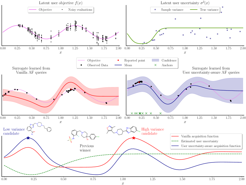
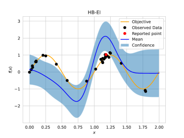
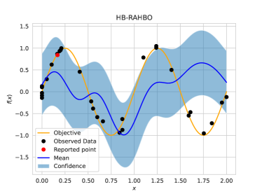
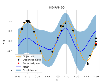
This flaw results in the PBO acquisition functions being risk-neutral, only seeking to optimize the statistics of latent utility value [16]. Consider the varying aleatoric uncertainty results in situations where the latent utility yields two solutions that deliver similar expected function values, yet one may be noisier (Figure 1). Choosing the noisier solution increases the risk of inconsistent preferential feedback from human experts. Over time, this inconsistency can result in suboptimal outcomes for PBO. Consequently, we advocate for adopting a risk-averse paradigm, necessitating a balance between maximizing the expected latent utility value and minimizing aleatoric uncertainty [28]. For example, a chemist might opt for slightly inferior quality molecules, but this leads to more confident preferential feedback. While there exist risk-averse variants of standard BO [28], this problem has not been studied for PBO.
2 Background
2.1 Preferential Bayesian optimization
The objective of PBO is to determine the optimal solution using the duel feedback , signifying a preference over . The preference structure is governed by the latent function , defined over a subset . As detailed in [9], the duel outcome is determined by
| (1) |
where , denote zero-mean additive noise capturing the human aleatoric uncertainty. PBO employs the preferential GP as a surrogate of the latent function in a probabilistic framework [41].
Most works in PBO commonly assume the homoscedastic setting, where the noise is drawn from a nondegenerate normal distribution , for all . While this assumption offers computational efficiency, it is unrealistic since humans may exhibit partial knowledge of the inputs, resulting in varying aleatoric uncertainty.
We argue the noise process should be input-dependent, capturing the user’s varying level of uncertainty across the inputs. Next, we recall how GPs work in the context of heteroscedastic noise.
Prior. We begin by placing a zero-mean Gaussian process prior to the latent function, , with a stationary kernel . Therefore, the GP prior density function over a finite set of output values is a multivariate Gaussian
| (2) |
where and is the kernel matrix.
Likelihood. Assume we have access to human observations of duel feedbacks , with and being the winner and the loser of the duel, respectively. Denoting , we have . Let be the concatenation of winners and losers from duels . The likelihood function adheres to a Gaussian cumulative density function (CDF) [9] defined as follows:
| (3) |
It is worth noticing that the likelihood addresses the entanglement of noises by incorporating both noise distribution variances as the normalizing factor for . In the homoscedastic setting, the noise variance and is a constant .
Posterior. Given the GP prior density function and likelihood , the posterior density function of the latent function conditioned on follows the Bayes’s theorem:
| (4) |
It is established that the exact posterior of the preference GP conforms to a skew GP [5].
Acquisition Function. Once the posterior has been obtained, BO employs an acquisition function (AF) to determine the next query to evaluate:
| (5) |
where is any function measuring the informativeness of . e.g., leads to the Expected Improvement. Common AFs are typically risk-neutral, focusing only on the epistemic uncertainty by maximizing against the posterior of the latent function. Conversely, our approach incorporates risk-averse AFs, adding the aleatoric uncertainty.
The other design of the pair is often taken as the winner of the previous duel or the current maximizer of the posterior mean. AFs optimizing for whole pairs have also been proposed [2].
2.2 Kernel density estimation
Let denote i.i.d. samples with probability density . Using , Kernel Density Estimation (KDE) estimates through the following formula:
| (6) |
Here, denotes a kernel function satisfying . The bandwidth is critical in estimating the density. A small bandwidth leads to a rough, spiky estimate, whereas a large bandwidth results in over-smoothing. A complete discussion on that matter can be found in [14]. Let us also mention input-specific bandwidth selection procedures such as [26]. If only takes non-negative values and is fixed, then is a probability density. We consider a Gaussian kernel for , which satisfies the latter assumption.
3 Preferential BO with heteroscedastic noise
To solve the heteroscedastic PBO problem introduced in Section 2.1, we explicitly model the aleatoric user uncertainty. Section 3.1, introduces a heteroscedastic noise distribution with input-dependent variance. That variance itself involves a distribution obtained by means of Kernel Density Estimation, constructed from a set of user-specified reliable inputs called anchors (Section 3.2). Next, Section 3.3 presents the Hallucination Believer, a method adapted from [41] and used to infer the proposed heteroscedastic preferential GP. Finally, the surrogate informs a risk-averse acquisition function described in Section 3.4. The whole process is summarized on a toy case in Figure 1.
–
3.1 Heteroscedastic noise distribution
Recall that vanilla PBO assumes the noise to be drawn from a normal distribution , characterized by a constant variance . We chose to model heteroscedastic noise as follows:
| (7) |
Here, is a scaling factor. Substituting the probability density for the uniform density leads to a homoscedastic noise distribution. Conversely, opting for a non-uniform probability density produces heteroscedastic noise distribution. Observe that the variance can be interpreted as a value estimation problem represented by an un-normalized energy-based model (EBM), with specifying the energy function. Notably, the desirable outputs correspond to high energy function values, resulting in low energy scores [27]. In the context of heteroscedastic PBO, it is important to determine the appropriate information conveyed by .
3.2 Anchors-based input-dependent noise
In general comparison tasks (including preference), humans exhibit partial knowledge of different inputs [37, 19, 12]. This partial knowledge encompasses easily comparable inputs, which is associated with a low human aleatoric uncertainty [37]. For the purposes of this research, we refer to these easily comparable inputs as reliable inputs. We consider to quantify the reliability of an input according to a human expert. However, the precise formulation of remains unclear.
To formalize our approach, we introduce anchors, a set of reliable inputs provided by the human expert. Humans are known to excel in identifying these reliable inputs [29, 4, 34]. We assume the anchors have been collected in an i.i.d. manner, ensuring each is treated equally. Comparing an input close to the anchors is relatively straightforward for a human expert. Therefore, the anchors encapsulate the region with high probability density . This implies that the noise drawn over these region exhibits low variance.
The anchors allow us to construct a proxy of the probability density . For this purpose, we perform KDE as formalized in Equation 6 to obtain the density estimator for all ,
| (8) |
where denotes input dimensionality. The estimator assigns a higher value when the proximity of to the anchors set increases. This proximity is represented by the Euclidian distance and a kernel with a specified bandwidth . Following Equation 7, we formulate the noise distribution :
| (9) |
where is a scaling factor. We assume that noise values across different inputs are independent, given the set of anchors. It is worth noticing that no further assumptions are required about the anchors. For instance, they do not have to be the inputs leading to a better optimum. Further details regarding the preferential likelihood under heteroscedastic noises, hyperparameter optimization, and time complexity of KDE can be found in Appendix A.
3.3 Hallucination believer for inference strategy
We adopt the hallucination believer (HB) [41] to perform inference in the heteroscedastic setting. Recall that the posterior distribution of the preferential GP is characterized as a skew GP, for which inference is notoriously challenging since it involves numerous evaluations of the Cumulative Distribution Function (CDF) of the multivariate normal distribution (MVN) [3]. Takeno et al. address this challenge by proposing the HB method, leveraging Gibbs sampling.
Recall the set of duels specified in Section 2.1. Takeno et al. [41] propose to generate a new sample , called the hallucination drawn from through Gibbs sampling. Note that the sample path from the skew GP denoted as for any output vector of the inputs follows an MVN distribution, implying a regular GP. This characteristic enables a proper posterior computation of , outperforming other approximate inference techniques like Laplace approximation. Nevertheless, we emphasize that the proposed noise distribution can be applied to any approximate inference method. The algorithm and details of the HB method are outlined in Algorithm 1 and Appendix B, respectively.
3.4 Risk-averse acquisition functions
In the decision-making theory, the aleatoric uncertainty can be interpreted as a form of risk [24]. In our case, we regard the noise variance as the embodiment of this risk as it is associated with the aleatoric uncertainty. It is noteworthy that variance is widely used for risk measurement [31, 22, 15]. To ensure robust querying of new candidates in the presence of heteroscedastic noise, we employ risk-averse acquisition functions that penalize high variance [28]. In essence, these acquisition functions trade off the informativeness of the latent function and the aleatoric uncertainty stemming from the reliability of human judgment.
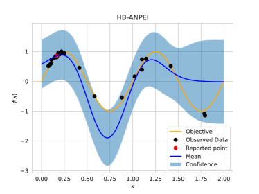
Specifically, we consider two known risk-averse acquisition functions , both leveraging the variance of noise distribution as the penalty criterion. The first one is the aleatoric noise-penalized expected improvement (ANPEI) [17] defined as
| (10) |
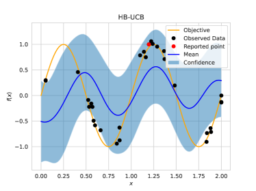
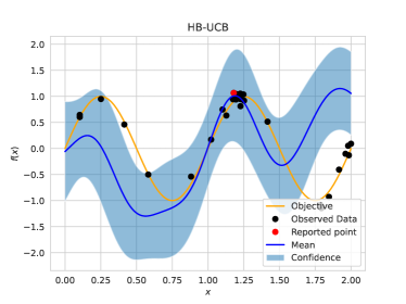
with and denote the incumbent best value and a scaling constant, respectively. As the actual value is not observed in PBO, the incumbent is usually replaced by the maximum posterior mean value over points in the previous queries [36]. Subsequently, we consider the risk-averse upper confidence bound (RAHBO) [28] as
| (11) |
The , denote the posterior mean and variance of the statistical surrogate accounting for the latent function , respectively. Additionally, are the scaling factors that control the influence of the variance of the latent function and the noise distribution, respectively.
4 Theoretical analysis
Risk analysis. Suppose we can access the true density for all . We are interested in assessing the consistency of the variance estimator in relation to the true variance. We approach this by analyzing the mean squared error (MSE) of the variance, denoted as . This analysis requires assumptions regarding the smoothness of the probability density function and the characteristic of the kernel under the integral operation, as described below.
Assumption 4.1
belongs to a class of densities defined as follows:
with denoting Hölder class. The kernel used in the KDE estimator is a kernel of order .
Theorem 4.2
Fix and take . Then, for any input and the number of anchors , the estimated variance satisfies
| (12) |
where is a constant depending on Hölder class parameter , constant , scaling factor , and the kernel bandwidth .
Of note, the Gaussian kernel satisfies the above assumption. The outline of the proof is as follows. We first bound the MSE of variance as a scaled MSE of density , leveraging Lipschitz-continuous property. We then derive the bound for MSE of the density through variance-bias decomposition. The theorem tells that the convergence rate of MSE shrinks polynomially w.r.t. the number of anchors . It implies that the estimator will be as accurate as the true variance with a sufficient number of anchors. However, the convergence rate is slow as we deal with higher data dimensionality . Consequently, the accuracy of the variance estimator diminishes with higher dimensions. The detailed proof of the theorem can be found in Appendix C.1.
Concentration analysis. Another way to assess the consistency is understanding the probability of deviating from the true variance .
Theorem 4.3
For any , there exist constants and , such that
| (13) |
for any . Furthermore, under an additional assumption, the following bound also holds.
| (14) |
for constants and depends on .
The proof employs Lipschitz continuous property to bound . Subsequently, we apply two types of concentration inequality by Bernstein [6] and Giné and Guillou [13]. The first inequality implies that close to with a high probability as increases. However, the probability shrinks as grows. The second inequality provides a stronger bound since this result holds uniformly over all . Obtaining this inequality requires the kernel to belong to a bounded measurable VC class. In addition, it restricts the value of as its behavior should depend on . The proof of the theorem can be found in Appendix C.2.
5 Related work
Bayesian optimization with heteroscedastic noise. In most real-world settings, defining the likelihood based on a fixed variance noise leads to misspecified posteriors, which can harm the optimization by suggesting designs incorrectly believed to yield high function values. Several attempts have been made to tackle this issue at acquisition level [28], surrogate level [10, 17] or by adapting distribution-free uncertainty quantification techniques like conformal inference to BO [38].
Preferential Bayesian optimization. Most of the works in BO revolve around two modeling choices: statistical surrogate and acquisition module. In PBO, the posterior is usually untractable, and hence, a seminal work proposed to carry inference using Laplace approximation [7]. Other works have leveraged the fact that the surrogate can be shown to be a skew GP, for which a posterior sampling scheme can be derived [5]. Approximate inference techniques such as Expectation-Propagation and MCMC have also been shown to work [41]. Let us also mention the existence of a PBO method that employs neural networks as a surrogate rather than GPs [20]. On the acquisition side, some work adapted classical acquisition functions to the PBO case by selecting one of the duel elements as the winner of the previous duel and optimizing for the second element using Expected Improvement or Thompson Sampling [36]. Next, acquisition functions leveraging the preferential nature of the queries were also proposed [16, 2]. Recent work has also investigated preferential relations and queries to encode and elicit user prior beliefs [23, 1]. To the best of our knowledge, employing heteroscedastic noise models to account for human uncertainty has not yet been explored in PBO.
Kernel density estimation in Bayesian optimization. Anchors-based modeling was previously introduced by Eduardo and Gutmann [11]. However, in this case, anchors referred to promising candidate solutions in the case of vanilla BO and were unrelated to human uncertainty in PBO like us. KDE was also employed to learn the distribution of contextual variables in BO [21].
6 Experiments
We thoroughly assess the performance of our approach on several synthetic black-box functions (Section 6.1). Next, we assess the performance of our method under various experiment and method settings (Section 6.2). These include for instance different distribution for the expert uncertainty, as well as different posterior inference techniques and hyperparameter optimization criteria.
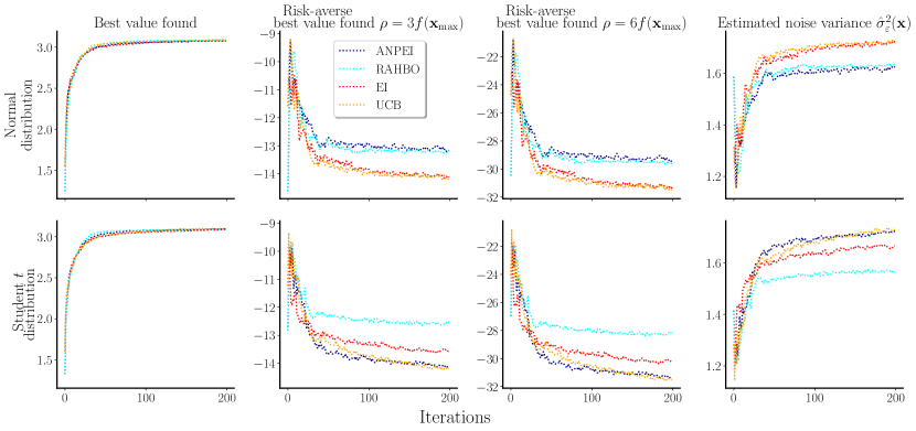
Baselines. Our proposed heteroscedastic PBO approach yields a surrogate explicitly modeling human aleatoric uncertainty. As such, this surrogate enhances vanilla acquisition functions, making them risk-averse. Thus, our method leads to two baselines: RAHBO and ANPEI, described in Equations 11 and 10, respectively. Concurrent baselines are risk-neutral versions of these AFs: UCB and EI. In all cases, the second design of the queried duel is obtained as the winner of the previous duel.
Implementation details. Unless stated otherwise, posterior inference for the statistical surrogate is carried out using the HB method presented in Sections 3.3 and B. The hyperparameters of the surrogate are obtained using marginal likelihood maximization. Regarding our KDE-based model of human aleatoric uncertainty, the estimation procedure for the bandwidth is detailed in Section A.2. All baselines use the same initial duels and anchors when applicable for the latter. The PBO trials are performed 30 times with different random seeds. All experiments were run on a private cluster consisting of a mixture of Intel®Xeon ®Gold 6248, Xeon ®Gold 6148, Xeon ®E5-2690 v3, and Xeon ®E5-2680 v3 processors. The longest experiments (Hartmann4) took a total of 24 hours.
Performance metrics. Several metrics are considered to assess each baseline’s performance. We follow Makarova et al. [28] and define the mean-variance objective , with the input acquired at round . Maximizing leads to queries that realize a tradeoff between high values and low variance, depending on how large is. One should notice that this objective involves the true variance , which is only accessible in synthetic examples. Our objective being defined, we report the risk-averse simple regret and cumulative regret , with the total number of BO rounds, and . Unless stated otherwise in dedicated experiments, we set . Lastly, we also report the standard simple and cumulative regrets and the best value found, all of which corresponds to .
6.1 Synthetic experiments
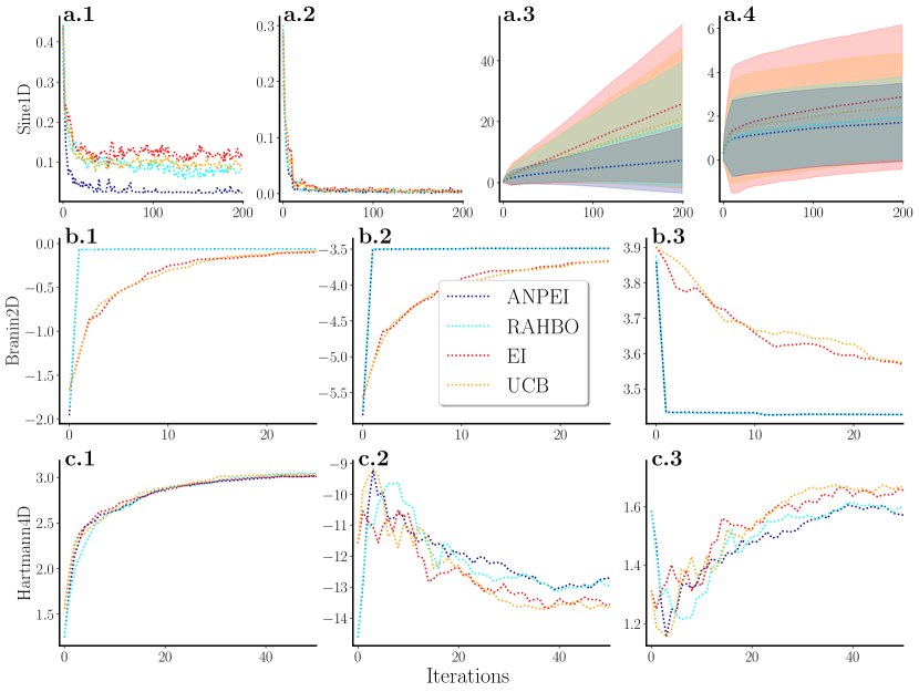
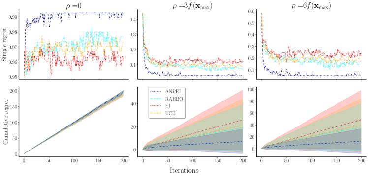
Sine function. We consider the sine function example presented in Figure 1. The input domain contains two similar optima . To simulate human-like aleatoric uncertainty, we construct an oracle by placing a normal distribution . We then utilize the oracle to specify the noise distribution and draw 30 anchors from it. The scaling factor for the noise variance estimator is set to . Figure 2a presents the results. For , panel (a.2) shows that all baselines quickly reach the best value in a similar fashion. However, when requiring the optimized queries to display a low variance, incentivized by setting , panel (a.1) shows that PBO-RAHBO and PBO-ANPEI exhibit lower risk-averse simple regret. The cumulative regret plots provided in panel (a.3-4) further demonstrate the superiority of risk-averse AFs, notably even when . Additional visualizations provided in Figures S1 and S2 illustrate how risk-averse AFs indeed lead to low-variance queries, contrarily to their risk-neutral counterparts.
Branin and Hartmann4. Next, we look at two classical black-box functions: Branin and Hartmann4. We simulate human aleatoric uncertainty by placing a normal distribution centered at points near and far from the optimum for the Branin and Hartmann4 functions, respectively. The scaling factor is set to and for Branin and Hartmann4, respectively. Panels (b) and (c) from Figure 2 report the mean-variance objective for (b.1 and c.1) and (b.2 and c.2). Lastly, (b.3) and (c.3) present the noise variance . Again, heteroscedastic PBO AFs prefer the query with lower variance, thus achieving higher risk-averse best value . Despite the lower variances, the queries obtained by heteroscedastic PBOs yield competitive best values found.
6.2 Ablation study
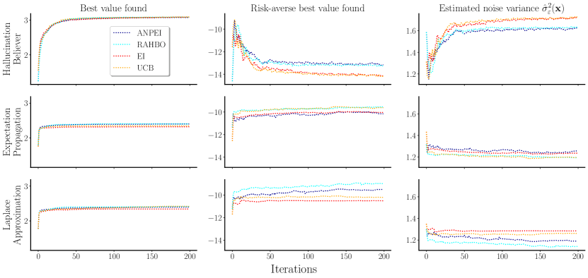
Posterior inference techniques. We evaluate the impact of different approximate inference methods on the outcomes of PBO. Specifically, we perform heteroscedastic PBO on the Hartmann4 function using both the Laplace approximation and expectation propagation. All other experimental settings remain as described above. Our heteroscedastic PBO consistently outperforms vanilla PBO in terms of mean-variance objective across inference techniques, without compromising the best value found.
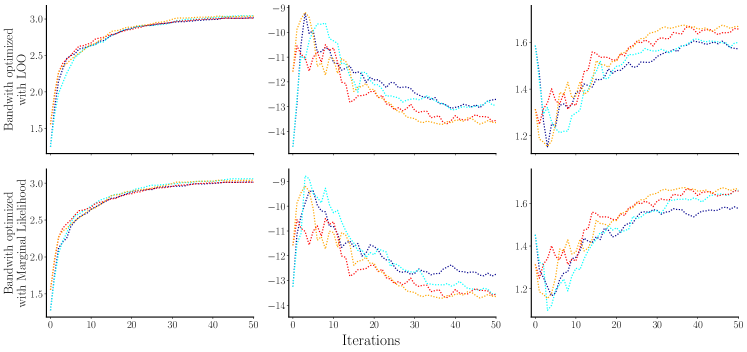
Bandwidth optimization method. Instead of optimizing the bandwidth of the estimator kernel using the marginal likelihood, we maximize the Leave-One-Out (LOO) criterion. Results indicate this approach does not impact simple and cumulative regret (Figure S3). However, the risk-averse simple and cumulative regret of PBO-RAHBO degrade compared to the main results. A similar study was carried for the Hartmann4 function in Section D.3 and yielded similar results.
Noise distributions. Lastly, we study the performance of heteroscedastic PBO under a non-Gaussian user uncertainty distribution . Specifically, we set as a student- density function with degrees of freedom. Our method remains consistent in terms of best value found (Figure S5). However, the objective PBO-ANPEI degrade compared to the main results. Further details can be found in Section D.4.
7 Conclusions
In this paper, we considered the problem of learning human preferences through dueling feedback between candidate pairs, a task that falls into the realm of Preferential Bayesian Optimization. Through several examples, we illustrated the necessity to account for the different levels of human uncertainty, as experts typically exhibit varying levels of knowledge over the input domain. To that end, we enhanced preferential GPs with an input-dependent noise model, built using a set of inputs over which the user has low uncertainty, so-called anchors. This led to faster convergence towards low-variance optima in BO trials, as we demonstrated in various synthetic examples.
Limitations and future work.
By bounding the MSE between the true noise variance and its estimator defined in Equation 9, Theorem 4.2 assesses how accurate the estimated user uncertainty is. and respectively lead to the true likelihood from Equation 3 and a “misspecified” likelihood, as the latter contains an estimate of the noise variance instead of the true one. Therefore, a promising research direction is to leverage Theorem 4.2 to derive the convergence rate of the misspecified likelihood to the true one. Additionally, releasing the i.i.d. assumption on the anchors set would allow their collection in a sequential manner.
References
- Adachi et al. [2023] Masaki Adachi, Brady Planden, David A. Howey, Krikamol Muandet, Michael A. Osborne, and Siu Lun Chau. Looping in the human: Collaborative and explainable bayesian optimization, 2023.
- Astudillo et al. [2023] Raul Astudillo, Zhiyuan Jerry Lin, Eytan Bakshy, and Peter Frazier. qeubo: A decision-theoretic acquisition function for preferential bayesian optimization. In Francisco Ruiz, Jennifer Dy, and Jan-Willem van de Meent, editors, Proceedings of The 26th International Conference on Artificial Intelligence and Statistics, volume 206 of Proceedings of Machine Learning Research, pages 1093–1114. PMLR, 25–27 Apr 2023. URL https://proceedings.mlr.press/v206/astudillo23a.html.
- Azzalini [2013] Adelchi Azzalini. The skew-normal and related families, volume 3. Cambridge University Press, 2013.
- Barsalou [1985] Lawrence W Barsalou. Ideals, central tendency, and frequency of instantiation as determinants of graded structure in categories. Journal of experimental psychology: learning, memory, and cognition, 11(4):629, 1985.
- Benavoli et al. [2021] Alessio Benavoli, Dario Azzimonti, and Dario Piga. Preferential bayesian optimisation with skew gaussian processes. In Proceedings of the Genetic and Evolutionary Computation Conference Companion, GECCO ’21, page 1842–1850, New York, NY, USA, 2021. Association for Computing Machinery. ISBN 9781450383516. doi: 10.1145/3449726.3463128. URL https://doi.org/10.1145/3449726.3463128.
- Bernstein [1924] Sergei Bernstein. On a modification of chebyshev’s inequality and of the error formula of laplace. Ann. Sci. Inst. Sav. Ukraine, Sect. Math, 1(4):38–49, 1924.
- Brochu et al. [2010] Eric Brochu, Vlad M Cora, and Nando De Freitas. A tutorial on bayesian optimization of expensive cost functions, with application to active user modeling and hierarchical reinforcement learning. arXiv preprint arXiv:1012.2599, 2010.
- Brusilovsky et al. [2007] Peter Brusilovsky, Alfred Kobsa, and Wolfgang Nejdl. The Adaptive Web - Methods and Strategies of Web Personalization. 01 2007. ISBN 978-3-540-72078-2. doi: 10.1007/978-3-540-72079-9.
- Chu and Ghahramani [2005] Wei Chu and Zoubin Ghahramani. Preference learning with gaussian processes. In Proceedings of the 22nd international conference on Machine learning, pages 137–144, 2005.
- Cowen-Rivers et al. [2022] Alexander Cowen-Rivers, Wenlong Lyu, Rasul Tutunov, Zhi Wang, Antoine Grosnit, Ryan-Rhys Griffiths, Alexandre Maravel, Jianye Hao, Jun Wang, Jan Peters, and Haitham Bou Ammar. Hebo: Pushing the limits of sample-efficient hyperparameter optimisation. Journal of Artificial Intelligence Research, 74, 07 2022.
- Eduardo and Gutmann [2023] Afonso Eduardo and Michael U. Gutmann. Bayesian optimization with informative covariance, 2023.
- Feltovic et al. [2001] Paul J Feltovic, Kenneth M Ford, and Robert R Hoffman. Expertise in context: Human and machine. AI Magazine, 22(3):62, 2001.
- Giné and Guillou [2002] Evarist Giné and Armelle Guillou. Rates of strong uniform consistency for multivariate kernel density estimators. In Annales de l’Institut Henri Poincare (B) Probability and Statistics, volume 38, pages 907–921. Elsevier, 2002.
- Goldenshluger and Lepski [2011] Alexander Goldenshluger and Oleg Lepski. Bandwidth selection in kernel density estimation: Oracle inequalities and adaptive minimax optimality. The Annals of Statistics, 39(3):1608 – 1632, 2011. doi: 10.1214/11-AOS883. URL https://doi.org/10.1214/11-AOS883.
- Golub and Tilman [2000] Bennett W Golub and Leo M Tilman. Risk management: approaches for fixed income markets, volume 73. John Wiley & Sons, 2000.
- González et al. [2017] Javier González, Zhenwen Dai, Andreas Damianou, and Neil D Lawrence. Preferential bayesian optimization. In International Conference on Machine Learning, pages 1282–1291. PMLR, 2017.
- Griffiths et al. [2021] Ryan-Rhys Griffiths, Alexander A Aldrick, Miguel Garcia-Ortegon, Vidhi Lalchand, et al. Achieving robustness to aleatoric uncertainty with heteroscedastic bayesian optimisation. Machine Learning: Science and Technology, 3(1):015004, 2021.
- Hastie et al. [2009] Trevor Hastie, Robert Tibshirani, Jerome H Friedman, and Jerome H Friedman. The elements of statistical learning: data mining, inference, and prediction, volume 2. Springer, 2009.
- Hoffman [2014] Robert R Hoffman. The psychology of expertise: Cognitive research and empirical AI. Psychology Press, 2014.
- Huang et al. [2023a] Daolang Huang, Louis Filstroff, Petrus Mikkola, Runkai Zheng, Milica Todorovic, and Samuel Kaski. Augmenting bayesian optimization with preference-based expert feedback. In ICML 2023 Workshop The Many Facets of Preference-Based Learning, 2023a. URL https://openreview.net/forum?id=OJXfwj2hiP.
- Huang et al. [2023b] Xiaobin Huang, Lei Song, Ke Xue, and Chao Qian. Stochastic bayesian optimization with unknown continuous context distribution via kernel density estimation, 2023b.
- Hull [2012] John Hull. Risk management and financial institutions,+ Web Site, volume 733. John Wiley & Sons, 2012.
- Hvarfner et al. [2023] Carl Hvarfner, Frank Hutter, and Luigi Nardi. A general framework for user-guided bayesian optimization, 2023.
- Kahneman and Tversky [2013] Daniel Kahneman and Amos Tversky. Prospect theory: An analysis of decision under risk. In Handbook of the fundamentals of financial decision making: Part I, pages 99–127. World Scientific, 2013.
- Koyama et al. [2020] Yuki Koyama, Issei Sato, and Masataka Goto. Sequential gallery for interactive visual design optimization. ACM Transactions on Graphics (TOG), 39(4):88–1, 2020.
- Kpotufe and Garg [2013] Samory Kpotufe and Vikas Garg. Adaptivity to local smoothness and dimension in kernel regression. In C.J. Burges, L. Bottou, M. Welling, Z. Ghahramani, and K.Q. Weinberger, editors, Advances in Neural Information Processing Systems, volume 26. Curran Associates, Inc., 2013. URL https://proceedings.neurips.cc/paper_files/paper/2013/file/28fc2782ea7ef51c1104ccf7b9bea13d-Paper.pdf.
- LeCun et al. [2006] Yann LeCun, Sumit Chopra, Raia Hadsell, M Ranzato, and Fujie Huang. A tutorial on energy-based learning. Predicting structured data, 1(0), 2006.
- Makarova et al. [2021] Anastasia Makarova, Ilnura Usmanova, Ilija Bogunovic, and Andreas Krause. Risk-averse heteroscedastic bayesian optimization. Advances in Neural Information Processing Systems, 34:17235–17245, 2021.
- Medin and Ortony [1989] Douglas L Medin and Andrew Ortony. Psychological essentialism. Similarity and analogical reasoning, 179:195, 1989.
- Nocedal [1980] Jorge Nocedal. Updating quasi-newton matrices with limited storage. Mathematics of computation, 35(151):773–782, 1980.
- Rachev et al. [2007] Svetlozar T Rachev, Stefan Mittnik, Frank J Fabozzi, Sergio M Focardi, et al. Financial econometrics: from basics to advanced modeling techniques. John Wiley & Sons, 2007.
- Rasmussen and Williams [2006] Carl Edward Rasmussen and Christopher K. I. Williams. Gaussian processes for machine learning. Adaptive computation and machine learning. MIT Press, 2006. ISBN 026218253X.
- Raykar et al. [2010] Vikas C Raykar, Ramani Duraiswami, and Linda H Zhao. Fast computation of kernel estimators. Journal of Computational and Graphical Statistics, 19(1):205–220, 2010.
- Ross [1989] Brian H Ross. Distinguishing types of superficial similarities: Different effects on the access and use of earlier problems. Journal of Experimental Psychology: Learning, memory, and cognition, 15(3):456, 1989.
- Sen [2020] Bodhisattva Sen. Introduction to Nonparametric Statistics. 2020.
- Siivola et al. [2021] Eero Siivola, Akash Kumar Dhaka, Michael Riis Andersen, Javier González, Pablo García Moreno, and Aki Vehtari. Preferential batch bayesian optimization. In 2021 IEEE 31st International Workshop on Machine Learning for Signal Processing (MLSP), pages 1–6, 2021. doi: 10.1109/MLSP52302.2021.9596494.
- Slovic and Tversky [1982] Paul Slovic and Amos Tversky. Judgment under uncertainty: Heuristics and biases. Cambridge University Press, 1982.
- Stanton et al. [2023] Samuel Stanton, Wesley Maddox, and Andrew Gordon Wilson. Bayesian optimization with conformal prediction sets. In Francisco Ruiz, Jennifer Dy, and Jan-Willem van de Meent, editors, Proceedings of The 26th International Conference on Artificial Intelligence and Statistics, volume 206 of Proceedings of Machine Learning Research, pages 959–986. PMLR, 25–27 Apr 2023. URL https://proceedings.mlr.press/v206/stanton23a.html.
- Stone [1974] Mervyn Stone. Cross-validatory choice and assessment of statistical predictions. Journal of the royal statistical society: Series B (Methodological), 36(2):111–133, 1974.
- Sundin et al. [2022] Iiris Sundin, Alexey Voronov, Haoping Xiao, Kostas Papadopoulos, Esben Jannik Bjerrum, Markus Heinonen, Atanas Patronov, Samuel Kaski, and Ola Engkvist. Human-in-the-loop assisted de novo molecular design. Journal of Cheminformatics, 14(1), 2022.
- Takeno et al. [2023] Shion Takeno, Masahiro Nomura, and Masayuki Karasuyama. Towards practical preferential bayesian optimization with skew gaussian processes. In International Conference on Machine Learning, pages 33516–33533. PMLR, 2023.
Appendix — Heteroscedastic Preferential Bayesian Optimization with Informative Noise Distributions
Outline.
The appendix is organized as follows. In Appendix A, further details regarding our proposed anchors-based noise model are provided. In Appendix B, we describe the Hallucination Believer algorithm used for inference and inspired from [41]. Next, Appendix C contains the proofs of Theorems 4.2 and 4.3. Appendix D displays additional figures supporting the experiments carried in the main text. Finally, Appendix E provides the mathematical expression of the test functions employed throughout the paper.
Appendix A Details of anchors-based input-dependent noise
We consider the settings in Section 2.1 for this model.
A.1 Likelihood
We derive the likelihood as follows:
| (S1) |
where and denotes the variance of noise and , respectively.
A.2 Hyperparameter optimization
We minimize the negative log marginal likelihood approximated with Laplace approximation for preferential GP hyperparameter optimization. This involves obtaining where we define as
| (S2) |
The first and second derivatives, respectively, are given by
| (S3) | |||
| (S4) | |||
| (S5) | |||
| (S6) |
The solution of the gradient provides . Subsequently, we introduce which depends on the inverse Hessian given at , i.e., . We utilize the Newton-Raphson method to obtain , following [9]. Given and , we construct the evidence as
| (S7) |
We then formulate the hyperparameter optimization problem as
| (S8) |
with denotes the hyperparameters. Specifically, denotes the length scale of preferential GP . We utilize L-BFGS-B [30] to obtain the solution of Equation S8.
Subsequently, we apply leave-one-out (LOO) [18] to optimize the KDE kernel bandwidth . Note that LOO is a special case of cross-validation, where the -fold is fixed to one. The rationale behind choosing LOO lies in the context of our study, where human expert input typically yields a small number of anchors. Consequently, utilizing -fold to one aligns with the constraints imposed by our data. Given the anchors and bandwidth , we aim to minimize the negative LOO, formulated as follows:
| (S9) |
For each anchor , we employ the remaining anchors to estimate . We then take the negative average of the logarithmic estimator for all anchors. We also employ L-BFGS-B to obtain .
According to Stone’s theorem, the Kernel Density Estimation (KDE) bandwidth derived through cross-validation converges to the optimal value [39]. This optimal bandwidth minimizes the Mean Squared Error (MSE) between the true density and the density estimator for all . Following this theorem, we obtain the following proposition.
Proposition A.1
Suppose that is bounded. Let denote the kernel variance estimator with bandwidth and let denote the bandwidth chosen by leave-one-out. Then,
| (S10) |
Note that we slightly abuse the notation of the estimator variance to differentiate the bandwidth being utilized. The result follows the Lipschitz continuous property of the noise variance shown as in the proof of Theorem 4.2.
A.3 Time complexity of KDE estimator
For a set of anchors with samples and evaluation inputs , the time complexity of the density estimator is [33]. This arises from constructing kernel matrix sized and the number of operations to obtain the density estimator for evaluation inputs. Note that this estimator does not hurt the time complexity of our preferential-GP-based latent function, which can lead to in the classical scenario [32].
Appendix B Details of Hallucination Believer algorithm
B.1 Posterior predictive distribution
We formalize the predictive posterior as follows. We first model the joint distribution between the test function and the sampled duels .
| (S11) | |||
| (S12) | |||
with , and is defined as in Section 2.1. It is worth noticing that is a diagonal matrix. We then rewrite the kernel matrix into a block of matrices as follows:
where , , . Thus, for an arbitrary output vector , we obtain
| (S13) | ||||
| (S14) | ||||
| (S15) |
B.2 Gibbs sampling for truncated MVN
Here, we provide the Gibbs sampling algorithm for truncated MVN distribution utilized to draw the hallucination sample in the HB algorithm.
Appendix C Proofs
C.1 Risk analysis
The proof begins by providing the definitions of Hölder class and the kernel of order , which are used to construct the necessary assumptions.
We first introduce multi-index notation as follows:
with , and denotes the magnitude of . Using multi-index notation, the derivative of a function is denoted by
Definition C.1
Assume that and let . The Hölder class on is defined as the set of times differentiable functions whose derivative satisfies
| (S16) |
with denotes the metric on .
Definition C.2
Let be an integer. We say that is a kernel of order if the functions are integrable and satisfy
| (S17) |
It is also important to introduce the notion of Lipschitz continuity as the foundation for our proofs.
Definition C.3
A function is Lipschitz-continuous if there exists such that
| (S18) |
with and denote the Lipschitz constant and metric on , respectively.
Subsequently, we mention all the propositions responsible for developing Lemma C.6. Later on, we also employ these propositions to prove Theorem 4.3. The propositions provide the bound for the variance and the bias of the KDE, respectively.
Proposition C.4
(Sen [35]) Suppose that the density satisfies for all . Let be the kernel such that
Then, for any and we have
| (S19) |
with .
Proposition C.5
The proof of Theorem 4.2 relies on the following lemma, which provides the bound of the MSE between the density estimator and the true probability density function whenever Assumption 4.1 holds.
Lemma C.6
Lemma C.6 obtains the bound by decomposing MSE as the addition of variance and bias squared. Subsequently, it leverages Proposition C.4 and Proposition C.5 to obtain the bound of variance and bias, respectively. Equipped with Lemma C.6, we can now state and prove Theorem 4.2.
See 4.2
Proof:
By invoking the definition of the variance of the noise distribution, we derive:
| (S22) |
Define the map for . is Lipschitz-continuous with Lipschitz constant . Furthermore, and are quantities bounded in for all . Then, the following bound holds:
| (S23) |
We then apply Lemma C.6 to obtain:
| (S24) |
The choice of is based on the optimum bandwidth of the regular KDE [35].
C.2 Concentration analysis
This analysis requires an assumption that depends on covering number. As a starting point, we define covering as follows.
Definition C.7
Let be a metric space and . is an covering of if , such that
Based on the definition above, covering number tells the number of -balls to cover a given space by allowing the overlaps between the balls. The formal definition of covering number is provided below.
Definition C.8
(covering number)
Here, we additionally assume the kernel belongs to a bounded measurable VC class, as described below.
Assumption C.9
The KDE kernel belongs to a collection of measurable functions , with satisfies
| (S25) |
where denotes the covering number of metric space , is the envelope function of , the constants are the VC characteristics of , and the supremum is taken over the set of all probability measures on .
Theorem 4.3 is built upon the following Lemmas. The first lemma is the renowned Bernstein’s inequality. The second lemma tells the appropriate value to guarantee the probability of KDE exponentially deviating from its expectation depending on the number of anchors as well as the dimensionality of the data [13].
Lemma C.10
(Bernstein [6]) Suppose that are i.i.d. random variables with mean , , and . Then for any , the following inequality holds.
| (S26) |
with denotes the sample mean.
Lemma C.11
Then for all large , Equation S27 holds with and are replaced by and , respectively.
We are now ready to prove Theorem 4.3.
See 4.3
Proof:
By invoking the definition of the noise variance and applying the triangle inequality, we derive the following bounds:
| (S29) |
The last inequality follows the Lipschitz continuous property as in the proof of Theorem 4.2. Next, we bound the second term using Proposition C.5, yielding . Subsequently, we address the first term of Section C.2. Define that with the random variable . Notably, where . Proposition C.4 provides . By applying Bernstein’s inequality, we obtain the following bound:
| (S30) |
whenever and . If we choose , then the following bound holds.
| (S31) |
Applying Equation S31 to Section C.2 results in Equation 13. To prove the second result, we can derive
| (S32) |
The third inequality follows the Lipschitz continuous property as in the proof of Theorem 4.2. By applying Lemma C.11 into Equation S32 and choose , such that where and satisfy Lemma C.11, then the following bound holds
| (S33) |
Applying Equation S33 to Equation S32 results in Equation 14.
Appendix D Additional experiments and visualizations
D.1 Further sine experiment visualizations
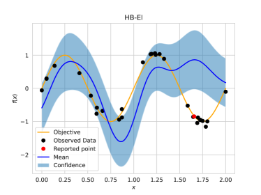
We provide additional visualizations for query acquisitions for sine experiments in Figure S1 and Figure S2. The visualizations demonstrate that PBO-UCB and PBO-EI prefer to exploit the region with higher noise variance. On the contrary, PBO-RAHBO and PBO-ANPEI acquire points with lower aleatoric uncertainty inherited in noise.

D.2 Sine experiments with bandwidth selection via leave-one-out
In this experiment, we maximize the leave-one-out (LOO) criterion to optimize the bandwidth of the estimator kernel while keeping all other settings consistent with the main experiments. The results indicate that this approach does not impact either simple or cumulative regret. However, the risk-averse simple and cumulative regret of PBO-ANPEI degrade compared to the main results.
D.3 Synthetic function experiments with bandwidth selection via marginal likelihood
We also perform an ablation study on Hartmann4. In this study, we simultaneously select the lengthscale of the preferential GP and the bandwidth by maximizing the marginal log-likelihood. All other settings are kept consistent with the main experiments. The results indicate that this approach does not impact the best value found. However, the objective PBO-RAHBO degrade compared to the main results.
D.4 Synthetic functions experiments with student-t noise distribution
In this experiment, we aim to study the performance of heteroscedastic PBO when is chosen to be less smooth. For the purpose of this experiment, we set to be a student-t density function with the degree of freedom set to 5. It is worth noting that as increases, the density becomes smoother, eventually converging to a normal distribution as approaches infinity. All other settings are kept consistent with the main experiments. The results indicate that this approach does not impact the best value found. However, the objective PBO-ANPEI degrade compared to the main results.
Appendix E Experiment details
Branin-2D function:
defined over .
Hartmann-4D function:
defined over .