Vacuum energy density for interacting real and complex scalar fields in a Lorentz symmetry violation scenario

Abstract

In this paper the vacuum energy density and generation of topological mass are investigated for a system of a real and complex scalar fields interacting with each other. In addition to that, it is also included the quartic self-interaction for each one of the fields. The condition imposed on the real field is the periodic condition, while the complex field obey a quasi-periodic condition. The system is placed in a scenario where the CPT-even aether-type Lorentz symmetry violation takes place. We allow that the Lorentz violation affects the fields with different intensities. The vacuum energy density, its loop correction, and the topological mass are evaluated analytically. It is also discussed the possibility of different vacuum states and their corresponding stability requirements, which depends on the conditions imposed on the fields, the interaction coupling constants and also the Lorentz violation parameters. The formalism used here to perform this investigation is the effective potential one, which is written as a loop expansion via path integral in quantum field theory.

I Introduction

The Casimir effect is one of the most interesting physical phenomenon which is of pure quantum nature. This effect was predicted by H. Casimir casimir1948attraction in 1948. The Casimir effect consists in a force of attraction that arises between two neutral parallel plates, placed in vacuum near to each other. The theoretical description of such a force lies in the framework of the electromagnetic quantum field theory. The force of attraction is due to modifications in the vacuum fluctuations of the associated field, as a consequence of the imposed boundary conditions on the plates. The first experimental attempt to detect the Casimir’s prediction dates back to Sparnaay in 1958 Sparnaay:1958wg , and ended up not having the required precision to confirm the phenomenon without doubt. It was only several decades later that the Casimir effect was confirmed by several high accuracy experiments bressi2002measurement ; kim2008anomalies ; lamoreaux1997demonstration ; lamoreaux1998erratum ; mohideen1998precision ; mostepanenko2000new ; wei2010results . Currently, it is known that not only the quantum vacuum modifications of the electromagnetic field can give rise to a force, that is, the phenomenon is also manifested for instance in the context of the scalar and fermionic quantum field theory, at least theoretically. Besides, the nontrivial topology of a given spacetime can also influence the quantum vacuum fluctuations in such a way that a vacuum force is induced bordag2009advances ; milton2001casimir ; mostepanenko1997casimir . In this sense, the basic concept of the Casimir effect has been expanded into a broader set of possibilities for the quantum vacuum fluctuations of the underlining field to be altered. As a consequence, it is common in these other scenarios to say that a Casimir-like effect occurs.

For example, the vacuum energy for a massive fermionic field confined between two points in one spatial dimension, with the MIT bag model boundary condition imposed, is considered in Ref. Saghian:2012zy , due to the influence of the nontrivial topology of the global monopole spacetime in Ref. Saharian:2003sp , and due to a fermionic chain in Ref. flachi2017sign . Considering scalar fields, a Casimir-like effect with the field subjected to a helix-like boundary condition with temperature corrections is considered in Ref. aleixo2021thermal and subjected to Robin boundary conditions in Ref. romeo2002casimir . In Ref. maluf2020casimir the vacuum energy for a real scalar field and the Elko neutral spinor field in a field theory at a Lifshitz fixed point is obtained and in Ref. Escobar:2023hzz it is investigated a Casimir-like effect in the classical geometry of two parallel conducting plates, in a noncommutative spacetime within a coherent state approach. A review on the Casimir effect and its generalizations can be found in Ref. bordag2009advances ; milton2001casimir ; mostepanenko1997casimir .

In its most standard approach, the investigation of Casimir-like effects is performed assuming that the Lorentz symmetry is preserved. However, attempts to build a high energy scale theory fails to preserve the Lorentz symmetry, even locally when we consider gravity. In this sense, there are two proposals for the Lorentz symmetry violation. One is described in the context of string theory in Ref. Kos , where non-vanishing vacuum expectation values of some vector gives rise to preferential directions in the spacetime. The other proposal is considered in the context of quantum gravity in Ref. hovrava2009quantum , where different properties of scales in the space and time are set, which yields an anisotropy between space and time. In the scenario which the Lorentz symmetry violation is allowed, the spacetime becomes anisotropic in some direction which includes the time one, with the anisotropy being determined mathematically by a constant unit four-vector. The modifications in the spacetime introduced by the Lorentz symmetry violation, combined with appropriate conditions, affect the energy modes of the quantum fields and, as a consequence, a nonzero vacuum force is induced. The Lorentz violation is a topic in which a great deal of attention has been given in the past years, mainly because it is an alternative to obtain new physics beyond the standard model. In Ref. Aj a Casimir-like effect for a scalar field in a scenario with Lorentz symmetry violation as consequence of the presence of a constant vector is investigated together with a helix-like boundary condition. The influence of a Lorentz violation to the vacuum energy of a massive scalar field at finite temperature effects and in the presence of an external magnetic field is investigated in Ref. Santos:2022tbq . In cruz2020casimir , an aether-type Lorentz symmetry violation theoretical model is considered to investigate a Casimir-like effect and the generation of topological mass associated with self-interacting massive scalar fields. A Casimir-like effect in a scenario with Lorentz violation and considering higher order derivatives was considered in Ref. dantas2023bosonic . Considering the context of string theory, the Lorentz symmetry violation is studied in the case of low-energy scale in Refs. PhysRevD.55.6760 ; PhysRevD.58.116002 ; Ani ; Carl ; Hew ; Ber ; Kost ; Anc ; Ber2 ; Alf ; Alf2 . Also in the context of string theory and low-energy scale scenarios with Lorentz violation, the vacuum energy is investigated in Refs. Obo ; Obo2 ; Mar ; Mar2 ; Esc .

Quantum fields found in nature are always interacting with each other. For that reason the study of the Casimir effect demands models with interactions so that the description of the physical phenomenon becomes more realistic. In this context, the first step is to consider a quartic self-interaction in building the model, which in fact has been done in a variate of works cruz2020casimir ; Aj ; toms1980symmetry ; porfirio2021ground . On the other hand, interacting real scalar fields are considered in toms1980interacting , being one field twisted and the other untwisted, for the investigation of symmetry breaking and mass generation. Using non-equilibrium quantum field theory, the quartic interaction between two scalar real quantum fields is considered in wang2022particle , in order to investigate the phenomenon of particle production from oscillating scalar backgrounds in a Friedmann-Lemaître-Robertson-Walker universe. In Ref. PhysRevB.77.115409 a thermodynamics Casimir-like effect is studied considering interacting field theories with zero modes and in Ref. article the thermal corrections to the vacuum energy in a Lorentz-breaking scalar field theory is investigated. Also, in Ref. Erdas:2021xvv , the author investigates the finite temperature Casimir-like effect due to a massive and charged scalar field under the influence of a constant magnetic field, in a Lorentz symmetry violation scenario. A Casimir-like effect and the generation of topological mass for a system of a real field interacting with a complex one has recently been considered in Ref. PhysRevD.107.125019 .

In the present paper we consider two scalar quantum fields, one real and the other complex, interacting via a quartic interaction and in addition, the self-interaction of each field is also present. The real field is subject to a periodic condition, while the components of the complex field are subjected to a quasi-periodic condition PhysRevD.107.125019 . The system is placed in a scenario where the CPT-even aether-type Lorentz symmetry violation takes place Car ; Gomes:2009ch ; Chatrabhuti:2009ew ; Aj . We allow that the violation occurs with different intensities on each field. The quasi-periodic condition plays an important role when one considers nanotubes or nanoloops for a quantum field feng2014casimir , for instance, if the phase angle is zero, it corresponds to metallic nanotubes, while the value of $\pm\frac{2\pi}{3}$ corresponds to a semiconductor nanotubes. In order to investigate the vacuum energy density for the mentioned system, we use the path integral formalism and construct the effective potential in terms of a loop expansion. This formalism was developed by Jackiw jackiw1974functional and allows us to obtain the vacuum energy density and its loop corrections and in addition, loop corrections to the mass of the field. The conditions on the fields are chosen so that we can focus attention on investigating the effect of all elements present in the system on the vacuum state of the real field. Within the path integral formalism, we will see that the only constant background complex field, after the loop expansion, compatible with the imposition of a quasi-periodic condition is the one that vanishes from the start, something that does not occur for the real field.

Before proceeding, let us point out that in Ref. Jaffe:2005vp the author argues that the origin of the Casimir effect relies on the interaction of the electromagnetic field with the physical properties of the plates, i.e., charges and currents. Hence, it is shown that the original Casimir result for the vacuum force can be obtained in a framework where it is not necessary to invoke the notion of quantum vacuum usually present in the standard quantum field theory approach. Although in the present work we dot not consider an interaction with possible physical properties associated with the conditions adopted, we think that it is always important to describe the Casimir’s original configuration as a motivation to pursue an investigation in other scenarios where modifications on the vacuum fluctuations of a quantum field takes place as a consequence of a finite length (volume), as in our case. Thus, in contrast with Ref. Jaffe:2005vp , we make use of the standard quantum field theory framework where the concept of quantum vacuum is present, and it is widely accepted, to investigate the system described in the previous paragraph. However, in order to avoid confusion, instead of using terminologies such as ‘Casimir energy density’, or ‘Casimir force’, we shall use the terminologies ‘vacuum energy density’ or ‘vacuum force’.

This paper is organized as follows: in Sec.II we review the main aspects of the path integral formalism to obtain the effective potential in the case of two interacting quantum fields, one real and the other complex. The interaction considered is the so called quartic interaction, that is, a product between the modulus square of the complex field and the square of the real field and, in addition, we also consider self-interaction for each field. The whole system is considered in a scenario where the CPT-even aether-type Lorentz symmetry violation takes place. In Sec.III, we consider the real and complex fields interacting with each other. The real field subject to the periodic condition, while the components of the complex field obey quasi-periodic condition. We assume that the Lorentz symmetry violation occurs in the $z$-direction, along which the conditions are imposed and the effects are stronger. Upon using the generalized zeta function technique, we obtain the effective potential of the system, which allows us to calculate the vacuum energy density, up to two-loop corrections, and the one-loop correction to the mass. It is also discussed the conditions for the stability of the possible vacuum states which guarantees a positive topological mass. In the end of this section we briefly discuss the effect of the Lorentz violation scenario considered in the $\tau$, $x$ and $y$ directions. In Sec.IV we present our conclusions. Throughout this paper we use natural units in which both the Planck constant and the speed of light are set equal to unit, that is, $\hslash=c=1$, and the metric signature is $\left(-,+,+,+\right)$.

II Effective potential for real and complex scalar fields with Lorentz violation

Here we consider a system composed of a real scalar field denoted by $\psi$, interacting with a complex field denoted by $\phi$. The interaction between the fields is represented by a term proportional to the product of the square of the real field and the modulus square of the complex field. This choice of interaction is justified since it preservers the discrete symmetry $\psi\rightarrow-\psi$ of the real field, and also the global symmetry $\phi\rightarrow e^{i\Theta}\phi$ of the complex field, which is important for the predicability of a given model Haber . We also include the self-interaction of each field, which is represented by terms proportional to the fourth power of each field. The system is placed in a scenario where the CPT-even aether-type Lorentz symmetry violation is allowed Car ; Gomes:2009ch ; Chatrabhuti:2009ew ; Aj . Moreover, we work with the Euclidean spacetime coordinates, with imaginary time greiner2013field .

The action describing the system mentioned above, in Euclidean coordinates, can be written as the following,

$$S_{\text{E}}\left[\psi,\varphi_{i}\right]=S_{\text{K}}\left[\psi,\varphi_{i}\right]+S_{\text{L-V}}\left[\psi,\varphi_{i}\right]+S_{\text{V}}\left[\psi,\varphi_{i}\right],$$ (1)

where $S_{\text{K}}\left[\psi\right]$ is the kinetic term with explicit form given by PhysRevD.107.125019 ,

$$S_{\text{K}}\left[\psi,\varphi_{i}\right]=\frac{1}{2}\int d^{4}x\left(\psi\square\psi+\sum_{i=1}^{2}\varphi_{i}\square\varphi_{i}\right).$$ (2)

Note that the complex field $\phi$ has been separeted into its two real components $\varphi_{i}$, $i=1,2$ ryder1996quantum ; PhysRevD.107.125019 . The D’Alembertian operator, $\square$, is written in Euclidean spacetime coordinates as

$$\square=\left(\partial_{\tau}^{2}+\mathbf{\nabla}^{2}\right).$$ (3)

The next term in Eq. (1) is the CPT-even aether-type Lorentz symmetry violation action which is given by Car ; Gomes:2009ch ; Chatrabhuti:2009ew ; Aj

$$S_{\text{L-V}}\left[\psi,\varphi_{i}\right]=\frac{1}{2}\int d^{4}x\left\{-\chi_{\psi}\left(u^{0}\partial_{0}\psi\right)^{2}+\chi_{\psi}\left(u^{i}\partial_{i}\psi\right)^{2}+\sum_{i=1}^{2}\left[-\chi_{\varphi}\left(u^{0}\partial_{0}\varphi_{i}\right)^{2}+\chi_{\varphi}\left(u^{j}\partial_{j}\varphi_{i}\right)^{2}\right]\right\}.$$ (4)

Note that in the above expression, $\chi_{\psi}$ and $\chi_{\varphi}$ characterize the Lorentz violation for each field, and they are supossed to be much smaller than unity. This way we allow the Lorentz violation to influence each field with different intensities. The unit vector $u^{\mu}$ determine the direction in which the violation occurs.

The last term composing the action of the system is the one which includes the self-interaction and the interaction between the fields, i.e.,

$$S_{\text{V}}\left[\psi,\varphi_{i}\right]=-\int d^{4}xU\left(\psi,\varphi\right),$$

$$U\left(\psi,\varphi\right)=\frac{\lambda_{\psi}+C_{1}}{4!}\psi^{4}+\frac{m^{2}+C_{2}}{2}\psi^{2}+\frac{\mu^{2}}{2}\varphi^{2}+\frac{g}{2}\varphi^{2}\psi^{2}+\frac{\lambda_{\varphi}}{4!}\varphi^{4}+C_{3}.$$ (5)

The masses of the real and the complex fields are denoted by $m$ and $\mu$, respectively, $\lambda_{\psi}$ and $\lambda_{\phi}$ are the constant couplings of self-interaction and $g$ is the coupling constant of the interaction between the fields. We also make use of the notation $\varphi^{2}=\varphi_{1}^{2}+\varphi_{2}^{2}$. The constants $C_{i}$ are the renormalization constants and its explicit form will be obtained in the renormalization process of the effective potential. Note that if we set $\chi_{\psi}$ and $\chi_{\varphi}$ to zero, we recover the action for the interacting fields written in PhysRevD.107.125019 .

The construction of the effective potential using the path integral approach is described in detail in Refs. jackiw1974functional ; ryder1996quantum ; toms1980symmetry (see also cruz2020casimir ; porfirio2021ground ; PhysRevD.107.125019 ). Here we present only the main steps necessary to our goals. The action written in Eq. (1), is now expanded about a fixed background $\Psi$, $\Phi_{i}$ that is, $\psi=\Psi+\chi$, $\varphi_{i}=\Phi_{i}+\varrho$, with $\chi$ and $\varrho$ representing quantum fluctuations. Since we are interested in the real field $\psi$, we seek the effective potential as a function only of $\Psi$, i.e., $V_{\mathrm{eff}}\left(\Psi\right)$. Then it is unnecessary to shift the components of the complex field $\phi$, this amounts to set $\Phi_{i}=0$ jackiw1974functional . This is because the only fixed background field $\Phi_{i}$ that can satisfy a quasi-periodic condition, as in Eq. (17), is the one that vanishes. So we are anticipating this fact. Note that, as a consequence, we do not need to include counter terms proportional to the powers of $\phi$. This matter is also treated in Ref. PhysRevD.107.125019 .

The expansion of the effective potential in powers of $\hslash$, up to order $\hslash^{2}$, can be written as,

$$V_{\mathrm{eff}}\left(\Psi\right)=V^{\left(0\right)}\left(\Psi\right)+V^{\left(1\right)}\left(\Psi\right)+V^{\left(2\right)}\left(\Psi\right).$$ (6)

The zero order term, $V^{\left(0\right)}\left(\Psi\right)$, describes the classical potential, i.e., the tree-level contribution,

$$V^{\left(0\right)}\left(\Psi\right)=U\left(\Psi\right)=\frac{\lambda_{\psi}+C_{1}}{4!}\Psi^{4}+\frac{m^{2}+C_{2}}{2}\Psi^{2}+C_{3},$$ (7)

while $V^{\left(1\right)}\left(\Psi\right)$ is the one-loop correction to the classical potential above and is written in terms of a path integral as toms1980interacting ; PhysRevD.107.125019 ,

$$V^{\left(1\right)}\left(\Psi\right)=-\frac{1}{\Omega_{4}}\ln\int\mathcal{D}\psi\mathcal{D}\varphi_{1}\mathcal{D}\varphi_{2}\exp\left\{-\frac{1}{2}\left[\left(\psi,\hat{A}\psi\right)+\left(\varphi_{1},\hat{B}\varphi_{1}\right)+\left(\varphi_{2},\hat{B}\varphi_{2}\right)\right]\right\},$$

$$\left(\psi,\hat{A}\psi\right)=\int d^{4}x\ \psi\left(x\right)\hat{A}\psi\left(x\right).$$ (8)

The quantity $\Omega_{4}$ is the 4-dimensional volume of the Euclidean spacetime, which depends on the conditions imposed on the fields. Note that since the fixed background field is $\Phi_{i}=0$, there are no crossing terms in the above exponential PhysRevD.107.125019 . The self-adjoint operators $\hat{A}$ and $\hat{B}$ are defined as,

$$\hat{A}=-\square-\chi_{\psi}u^{0}u^{0}\partial_{0}\partial_{0}+\chi_{\psi}u^{i}u^{j}\partial_{i}\partial_{j}+m^{2}+\frac{\lambda_{\psi}}{2}\Psi^{2},$$

$$\hat{B}=-\square-\chi_{\varphi}u^{0}u^{0}\partial_{0}\partial_{0}+\chi_{\varphi}u^{i}u^{j}\partial_{i}\partial_{j}+\mu^{2}+g\Psi^{2}.$$ (9)

The one-loop correction to the effective potential can be written in terms of the generalized zeta function constructed from the eigenvalues of the operators $\hat{A}$ and $\hat{B}$ toms1980interacting ; PhysRevD.107.125019 . Denoting by $\alpha_{\sigma}$ and $\beta_{\rho}$, the eigenvalues of the operators $\hat{A}$ and $\hat{B}$, respectively, we can construct the generalized zeta functions in the following manner,

$$\zeta_{\alpha}\left(s\right)=\sum_{\sigma}\alpha_{\sigma}^{-s},\ \qquad\qquad\qquad\zeta_{\beta}\left(s\right)=\sum_{\rho}\beta_{\rho}^{-s},$$ (10)

where $\sigma$ and $\rho$ denote sets of quantum numbers associated with the eigenfunctions of the operators $\hat{A}$ and $\hat{B}$, respectively. The summation symbol stands for sum or integration of the quantum numbers, depending on whether they are discrete or continuous. Once we construct the generalized zeta functions in Eq. (10), we write the one-loop correction to the effective potential as below toms1980symmetry ; PhysRevD.107.125019 ; hawking1977zeta ,

$$V^{\left(1\right)}\left(\Psi\right)=V_{\alpha}^{\left(1\right)}\left(\Psi\right)+V_{\beta}^{\left(1\right)}\left(\Psi\right),$$

$$V_{\alpha}^{\left(1\right)}=-\frac{1}{2\Omega_{4}}\left[\zeta_{\alpha}^{\prime}\left(0\right)+\zeta_{\alpha}\left(0\right)\ln\nu^{2}\right],$$

$$V_{\beta}^{\left(1\right)}=-\frac{1}{\Omega_{4}}\left[\zeta_{\beta}^{\prime}\left(0\right)+\zeta_{\beta}\left(0\right)\ln\nu^{2}\right].$$ (11)

The notation $\zeta_{\alpha,\beta}\left(0\right)$ and $\zeta_{\alpha,\beta}^{\prime}\left(0\right)$ stands for the generalized zeta function and its derivative with respect to $s$ evaluated at zero, respectively. The parameter $\nu$ has dimension of mass and it is an integration measure in the functional space, which will be removed via renormalization of the effective potential toms1980symmetry ; toms1980interacting ; PhysRevD.107.125019 . It is convenient to calculate the two-loop correction, $V^{\left(2\right)}\left(\Psi\right)$, of the effective potential from the two-loop Feynman graph. This correction can also be written it in terms of the generalized zeta function if one is interested in calculating only the vacuum contribution cruz2020casimir ; porfirio2021ground . We postpone the explicit form of the $V^{\left(2\right)}\left(\Psi\right)$ until Section III.2.

Once we obtain the effective potential and its corrections, we have to perform the renormalization. The renormalization process consists in the application of the following set of conditions:

$$\left.\frac{d^{4}V_{\mathrm{eff}}\left(\Psi\right)}{d\Psi^{4}}\right|_{\Psi=M}=\lambda_{\psi},$$ (12)

$$\left.\frac{d^{2}V_{\mathrm{eff}}\left(\Psi\right)}{d\Psi^{2}}\right|_{\Psi=v}=m^{2},$$ (13)

$$\left.V_{\mathrm{eff}}\left(\Psi\right)\right|_{\Psi=0}=0.$$ (14)

The first renormalization condition, Eq. (12), is written in analogy to Coleman-Weinberg coleman1973radiative , fixing the constant $C_{1}$ in Eq. (1) and also the coupling constant $\lambda_{\psi}$. $M$ is a parameter with dimension of mass and can be taken to be zero if the theory involves only massive fields cruz2020casimir ; porfirio2021ground ; Aj ; PhysRevD.107.125019 . The renormalization constant $C_{3}$ is fixed by the condition (14), while the condition in Eq. (13) fix the constant $C_{2}$ in Eq. (1), and $\Psi=v$ is the value of the field that minimizes the potential as long as the extremum condition is obeyed, that is,

$$\left.\frac{dV_{\mathrm{eff}}\left(\Psi\right)}{d\Psi}\right|_{\Psi=v}=0.$$ (15)

In the Sec. III.4 we discuss the vacuum stability and present the values of the field which satisfy the condition above. The last condition, Eq. (14), is used only in a massive field theory cruz2020casimir . The renormalization conditions presented in Eqs. (12), (13) and (14) are to be taken in the limit of Minkowski spacetime with no conditions imposed.

Now we are well equiped to investigate the loop-expansion of the effective potential, the generation of topological mass and the vacuum stability for the system of a real field interacting with a complex field. We will impose periodic condition for the real field, and quasi-periodic condition for the components of the complex field as well as consider a Lorentz symmetry violation for each field.

III Periodic and quasi-periodic conditions with Lorentz violation

The action of the system considered here has been written in Eq. (1). The real field is subjected to a periodic condition, while the components of the complex field obey a quasi-periodic condition. In addition, we assume that the Lorentz symmetry violation occur in the $z$-direction, which amounts to set the unit vector as $u^{\mu}=\left(0,0,0,1\right)$, the same direction along which the conditions are imposed. In this configuration, the Lorentz violation is expected to be nontrivial in comparison with the other directions cruz2020casimir ; Aj .

Since the real field is subject to the periodic condition together with the Lorentz symmetry violation in the $z$-direction, the eigenvalues of the operator $\hat{A}$, presented in Eq. (9), are found to be Aj ; PhysRevD.107.125019 ,

$$\alpha_{\sigma}=k_{\tau}^{2}+k_{x}^{2}+k_{y}^{2}+\left(1-\chi_{\psi}\right)\left(\frac{2\pi n}{L}\right)^{2}+M_{\lambda}^{2},$$

$$M_{\lambda}^{2}=m^{2}+\frac{\lambda_{\psi}}{2}\Psi^{2},\ \ n=0,\pm 1,\pm 2,...,$$ (16)

where $L$ is the periodic parameter, which compactifies the $z$-coordinate into a length $L$. The subscript $\sigma$ stands for the set of quantum numbers $\left(k_{\tau},k_{x},k_{y},n\right)$.

The components of the complex field are subject to a quasi-periodic condition as well as to the Lorentz symmetry violation feng2014casimir ; porfirio2021ground ; Aj ; PhysRevD.107.125019 , which leads to the following set of eigenvalues of the operator $\hat{B}$, presented in Eq. (9),

$$\beta_{\rho} = p_{\tau}^{2}+p_{x}^{2}+p_{y}^{2}+\left(1-\chi_{\varphi}\right)\left(\frac{2\pi}{L}\right)^{2}\left(n+\eta\right)^{2}+M_{g}^{2},$$

$$M_{g}^{2} = \mu^{2}+g\Psi^{2},\ \ n=0,\pm 1,\pm 2,....$$ (17)

Here $\rho$ stands for the set of quantum numbers $\left(p_{\tau},p_{x},p_{y},n\right)$. Moreover, the allowed values of the phase $\eta$ are in the interval $0\leq\eta<1$. Note that if we set $\eta=0$, then the field components $\varphi_{i}$ are called untwisted scalar fields and, if $\eta=1/2$ we are in the twisted field case toms1980interacting .

Once we know the explicit form of the eigenvalues $\alpha_{\sigma}$ and $\beta_{\rho}$, given in Eqs. (16) and (17), respectively, we construct the generalized zeta function, Eq. (10), and obtain a useful expression for the first order correction to the effetive potential, Eq. (11). The vacuum energy density and also the topological mass are obtained from the renormalized effective potential which in turn is obtained from effective potential after the application of the renormalization conditions. In the next section we shall obtain the renormalized effective potential, up to first order correction, and the vacuum energy density.

III.1 One-loop correction and the vacuum energy density

We start considering first the one-loop correction from the real field $\psi$. The eigenvalues used to construct the generalized zeta function, Eq. (10), are presented in Eq. (16). Therefore, the generalized zeta function takes the following form:

$$\zeta_{\alpha z}\left(s\right)=\frac{\Omega_{3}}{\left(2\pi\right)^{3}}\int dk_{\tau}dk_{x}dk_{y}\sum_{n=-\infty}^{+\infty}\left\{k_{\tau}^{2}+k_{x}^{2}+k_{y}^{2}+\left(1-\chi_{\psi}\right)\left(\frac{2\pi n}{L}\right)^{2}+M_{\lambda}^{2}\right\}^{-s},$$ (18)

where $\Omega_{3}$ represents the 3-volume associated with the Euclidean spacetime coordinates $\tau,x,z$, necessary to make the integrals dimensionless. The subscript $z$ is to remind that we are in the case where the Lorentz violation occur in the $z$-direction. In order to obtain a practical expression for the generalized zeta function (18), we take similar steps as the ones presented in porfirio2021ground ; PhysRevD.107.125019 , hence, we shall indicate the main steps. The first one is to use the following identity,

$$w^{-s}=\frac{2}{\Gamma\left(s\right)}\int_{0}^{\infty}d\tau\ \tau^{2s-1}e^{-w\tau^{2}},$$ (19)

and then perform the resulting Gaussians integrals in $k_{\tau}$, $k_{x}$ and $k_{y}$. After that, we identify the integral representation of the gamma function $\Gamma\left(z\right)$ abramowitz1965handbook ,

$$\frac{\Gamma\left(z\right)}{2}=\int_{0}^{\infty}d\mu\ \mu^{2z-1}e^{-\mu^{2}},$$ (20)

yielding the following form of the generalized zeta function,

$$\zeta_{\alpha z}\left(s\right)=\frac{\Omega_{4}\pi^{\frac{3}{2}-2s}}{2^{2s}L^{4-2s}}\frac{\Gamma\left(s-\frac{3}{2}\right)}{\Gamma\left(s\right)}\left(1-\chi_{\psi}\right)^{\frac{3}{2}-s}\sum_{n=-\infty}^{+\infty}\left[n^{2}+\left(\frac{M_{\lambda}L}{2\pi\sqrt{1-\chi_{\psi}}}\right)^{2}\right]^{\frac{3}{2}-s}.$$ (21)

In the above expression, $\Omega_{4}$ is the 4-dimensional volume in Euclidean spacetime, which takes into account the spacetime topology. In the case under consideration, the 4-dimensional volume is written as $\Omega_{4}=\Omega_{3}L$. The sum in Eq. (21) is performed via the folowing analytic continuation of the inhomogeneous, generalized Epstein function elizalde1995zeta ; feng2014casimir ; PhysRevD.107.125019 :

$$\sum_{n=-\infty}^{+\infty}\left[\left(n+\vartheta\right)^{2}+\kappa^{2}\right]^{-z}=\frac{\pi^{\frac{1}{2}}\kappa^{1-2z}}{\Gamma\left(z\right)}\left\{\Gamma\left(z-\frac{1}{2}\right)+4\left(\pi\kappa\right)^{z-\frac{1}{2}}\sum_{j=1}^{\infty}j^{z-\frac{1}{2}}\cos\left(2\pi j\vartheta\right)K_{\left(\frac{1}{2}-z\right)}\left(2\pi j\kappa\right)\right\},$$ (22)

where $K_{\gamma}(x)$ is the modified Bessel function of the second kind or, as it is also known, the Macdonald function abramowitz1965handbook . With the help of Eq. (22), one obtains the generalized zeta function, Eq. (21), in a practical form, i.e.,

$$\zeta_{\alpha z}\left(s\right)=\frac{\Omega_{4}}{2^{4}\pi^{2}}\frac{M_{\lambda}^{4-2s}}{\sqrt{1-\chi_{\psi}}\Gamma\left(s\right)}\left\{\Gamma\left(s-2\right)+2^{4-s}\sum_{j=1}^{\infty}f_{\left(2-s\right)}\left(\frac{jM_{\lambda}L}{\sqrt{1-\chi_{\psi}}}\right)\right\},$$ (23)

where we have defined the function $f_{\gamma}\left(x\right)$ as the ratio

$$f_{\gamma}\left(x\right)=\frac{K_{\gamma}\left(x\right)}{x^{\gamma}}.$$ (24)

Therefore, the one-loop correction $V_{\alpha z}^{\left(1\right)}\left(\Psi\right)$, Eq. (11), to the effective potential associated with the real field is written in the form

$$V_{\alpha z}^{\left(1\right)}\left(\Psi\right)=\frac{M_{\lambda}^{4}}{2^{6}\pi^{2}\sqrt{1-\chi_{\psi}}}\left[\ln\left(\frac{M_{\lambda}^{2}}{\nu^{2}}\right)-\frac{3}{2}\right]-\frac{M_{\lambda}^{4}}{2\pi^{2}\sqrt{1-\chi_{\psi}}}\sum_{j=1}^{\infty}f_{2}\left(\frac{jM_{\lambda}L}{\sqrt{1-\chi_{\psi}}}\right).$$ (25)

The expression above is the first order correction, that is, the one-loop correction to the effective potential due to the real field subject to the periodic condition, with Lorentz symmetry violation in the $z$-direction. Now we have to calculate the contribution due to the complex field.

The eigenvalues of the operator $\hat{B}$, associated with the complex field components are presented in Eq. (17) and leads to the following generalized zeta function,

$$\zeta_{\beta z}\left(s\right)=\frac{\Omega_{3}}{\left(2\pi\right)^{3}}\int dp_{\tau}dp_{x}dp_{y}\sum_{n=-\infty}^{+\infty}\left[p_{\tau}^{2}+p_{x}^{2}+p_{y}^{2}+\left(1-\chi_{\varphi}\right)\left(\frac{2\pi}{L}\right)^{2}\left(n+\eta\right)^{2}+M_{g}^{2}\right]^{-s}.$$ (26)

A simplified expression for $\zeta_{\beta z}\left(s\right)$ can be obtained in a similar way as the previous one porfirio2021ground ; PhysRevD.107.125019 . Therefore we present the final form of the generalized zeta function $\zeta_{\beta z}\left(s\right)$,

$$\zeta_{\beta z}\left(s\right)=\frac{\Omega_{4}}{2^{4}\pi^{2}}\frac{M_{g}^{4-2s}}{\sqrt{1-\chi_{\varphi}}\Gamma\left(s\right)}\left\{\Gamma\left(s-2\right)+2^{4-s}\sum_{j=1}^{\infty}\cos\left(2\pi j\eta\right)f_{\left(2-s\right)}\left(\frac{jM_{g}L}{\sqrt{1-\chi_{\varphi}}}\right)\right\}.$$ (27)

Calculating the zeta function above and its derivative at $s=0$, we find the one-loop correction to the effective potential, Eq. (11), due to the complex field as

$$V_{\beta z}^{\left(1\right)}\left(\Psi\right)=\frac{M_{g}^{4}}{2^{5}\pi^{2}\sqrt{1-\chi_{\varphi}}}\left[\ln\left(\frac{M_{g}^{2}}{\nu^{2}}\right)-\frac{3}{2}\right]-\frac{M_{g}^{4}}{\pi^{2}\sqrt{1-\chi_{\varphi}}}\sum_{j=1}^{\infty}\cos\left(2\pi j\eta\right)f_{\left(2\right)}\left(\frac{jM_{g}L}{\sqrt{1-\chi_{\varphi}}}\right).$$ (28)

Collecting the results presented in Eqs. (25) and (28), one can write the first order, or the one-loop correction to the effective potential in the following form,

$$V_{z}^{\left(1\right)}\left(\Psi\right)=\frac{M_{\lambda}^{4}}{2^{6}\pi^{2}\sqrt{1-\chi_{\psi}}}\left[\ln\left(\frac{M_{\lambda}^{2}}{\nu^{2}}\right)-\frac{3}{2}\right]+\frac{M_{g}^{4}}{2^{5}\pi^{2}\sqrt{1-\chi_{\varphi}}}\left[\ln\left(\frac{M_{g}^{2}}{\nu^{2}}\right)-\frac{3}{2}\right]$$

$$-\frac{M_{\lambda}^{4}}{2\pi^{2}\sqrt{1-\chi_{\psi}}}\sum_{n=1}^{\infty}f_{2}\left(\frac{nM_{\lambda}L}{\sqrt{1-\chi_{\psi}}}\right)-\frac{M_{g}^{4}}{\pi^{2}\sqrt{1-\chi_{\varphi}}}\sum_{j=1}^{\infty}\cos\left(2\pi j\eta\right)f_{2}\left(\frac{jM_{g}L}{\sqrt{1-\chi_{\varphi}}}\right).$$ (29)

Therefore, the nonrenormalized effective potential, Eq. (11), up to order $\hslash$, reads,

$$V_{\mathrm{eff}}\left(\Psi\right)_{z}=\frac{m^{2}+C_{2}}{2}\Psi^{2}+\frac{\lambda_{\psi}+C_{1}}{4!}\Psi^{4}+C_{3}$$

$$+\frac{M_{\lambda}^{4}}{2^{6}\pi^{2}\sqrt{1-\chi_{\psi}}}\left[\ln\left(\frac{M_{\lambda}^{2}}{\nu^{2}}\right)-\frac{3}{2}\right]+\frac{M_{g}^{4}}{2^{5}\pi^{2}\sqrt{1-\chi_{\varphi}}}\left[\ln\left(\frac{M_{g}^{2}}{\nu^{2}}\right)-\frac{3}{2}\right]$$

$$-\frac{M_{\lambda}^{4}}{2\pi^{2}\sqrt{1-\chi_{\psi}}}\sum_{n=1}^{\infty}f_{2}\left(\frac{nM_{\lambda}L}{\sqrt{1-\chi_{\psi}}}\right)-\frac{M_{g}^{4}}{\pi^{2}\sqrt{1-\chi_{\varphi}}}\sum_{j=1}^{\infty}\cos\left(2\pi j\eta\right)f_{2}\left(\frac{jM_{g}L}{\sqrt{1-\chi_{\varphi}}}\right).$$ (30)

The renormalization constants $C_{i}$ are obtained by applying the renormalization conditions expressed in the Eqs. (12), (13) and (14), in the limit of Minkowski spacetime, $L\rightarrow\infty$. The explicit form of the $C_{i}$’s are

$$C_{1}=\frac{6\lambda_{\psi}^{2}}{2^{6}\pi^{2}\sqrt{1-\chi_{\psi}}}\ln\left(\frac{\nu^{2}}{m^{2}}\right)+\frac{24g^{2}}{2^{5}\pi^{2}\sqrt{1-\chi_{\varphi}}}\ln\left(\frac{\nu^{2}}{\mu^{2}}\right),$$

$$C_{2}=\frac{2\lambda_{\psi}m^{2}}{2^{6}\pi^{2}\sqrt{1-\chi_{\psi}}}\left[\ln\left(\frac{\nu^{2}}{m^{2}}\right)+1\right]+\frac{4g\mu^{2}}{2^{5}\pi^{2}\sqrt{1-\chi_{\varphi}}}\left[\ln\left(\frac{\nu^{2}}{\mu^{2}}\right)+1\right],$$

$$C_{3}=\frac{m^{4}}{2^{6}\pi^{2}\sqrt{1-\chi_{\psi}}}\left[\ln\left(\frac{\nu^{2}}{m^{2}}\right)+\frac{3}{2}\right]+\frac{\mu^{4}}{2^{5}\pi^{2}\sqrt{1-\chi_{\varphi}}}\left[\ln\left(\frac{\nu^{2}}{\mu^{2}}\right)+\frac{3}{2}\right].$$ (31)

Note that all coefficients above depend on the Lorentz violation parameters $\chi_{\psi}$ and $\chi_{\varphi}$. Upon substituting the renormalization constants above into the effective potential, Eq. (30), we obtain the renormalized effective potential for a system of interacting scalar fields with the Lorentz violation in the $z$-direction:

$$V_{\mathrm{eff}}^{R}\left(\Psi\right)_{z}=\frac{m^{2}}{2}\Psi^{2}+\frac{\lambda_{\psi}}{4!}\Psi^{4}+\frac{m^{4}}{2^{6}\pi^{2}\sqrt{1-\chi_{\psi}}}\ln\left(\frac{M_{\lambda}^{2}}{m^{2}}\right)+\frac{\mu^{4}}{2^{5}\pi^{2}\sqrt{1-\chi_{\varphi}}}\ln\left(\frac{M_{g}^{2}}{\mu^{2}}\right)$$

$$+\frac{\lambda_{\psi}^{2}\Psi^{4}}{2^{8}\pi^{2}\sqrt{1-\chi_{\psi}}}\left[\ln\left(\frac{M_{\lambda}^{2}}{m^{2}}\right)-\frac{3}{2}\right]+\frac{\lambda_{\psi}m^{2}\Psi^{2}}{2^{6}\pi^{2}\sqrt{1-\chi_{\psi}}}\left[\ln\left(\frac{M_{\lambda}^{2}}{m^{2}}\right)-\frac{1}{2}\right]$$

$$+\frac{g^{2}\Psi^{4}}{2^{5}\pi^{2}\sqrt{1-\chi_{\varphi}}}\left[\ln\left(\frac{M_{g}^{2}}{\mu^{2}}\right)-\frac{3}{2}\right]+\frac{g\mu^{2}\Psi^{2}}{2^{4}\pi^{2}\sqrt{1-\chi_{\varphi}}}\left[\ln\left(\frac{M_{g}^{2}}{\mu^{2}}\right)-\frac{1}{2}\right]$$

$$-\frac{M_{\lambda}^{4}}{2\pi^{2}\sqrt{1-\chi_{\psi}}}\sum_{n=1}^{\infty}f_{2}\left(\frac{nM_{\lambda}L}{\sqrt{1-\chi_{\psi}}}\right)-\frac{M_{g}^{4}}{\pi^{2}\sqrt{1-\chi_{\varphi}}}\sum_{j=1}^{\infty}\cos\left(2\pi j\eta\right)f_{2}\left(\frac{jM_{g}L}{\sqrt{1-\chi_{\varphi}}}\right).$$ (32)

The vacuum energy density is evaluated in a straightforward way once we know the explicit form of the renormalized effective potential presented in Eq. (32). Although there are in fact three possible vacuum, as we will se in section III.4, here we consider the vacuum state as $\Psi=0$. Hence, the vacuum energy density is obtained by taking $\Psi=0$ in the renormalized effective potential, i.e.,

$$\mathcal{E}_{0z}=\left.V_{\mathrm{eff}}^{R}\left(\Psi\right)_{z}\right|_{\Psi=0}=-\frac{m^{4}}{2\pi^{2}\sqrt{1-\chi_{\psi}}}\sum_{n=1}^{\infty}f_{2}\left(\frac{nmL}{\sqrt{1-\chi_{\psi}}}\right)-\frac{\mu^{4}}{\pi^{2}\sqrt{1-\chi_{\varphi}}}\sum_{j=1}^{\infty}\cos\left(2\pi j\eta\right)f_{2}\left(\frac{j\mu L}{\sqrt{1-\chi_{\varphi}}}\right).$$ (33)

The first term on the r.h.s of Eq. (33) is the contribution to the vacuum energy density from the real field $\psi$ under periodic condition, while the second term is the contribution from the complex field components, which is twice the contribution from one Klein-Gordon field under quasi-periodic condition porfirio2021ground . Obviously these two terms shows the dependence on the Lorentz violation parameters. Recalling that the Lorentz violation occurs in the $z$-direction, and comparing with the result obtained in Ref. PhysRevD.107.125019 we see the difference in the multiplicative factor in the form $\left(1-\chi\right)^{-\frac{1}{2}}$ which is also present in the argument of the Macdonald function, for each field contribution separately.

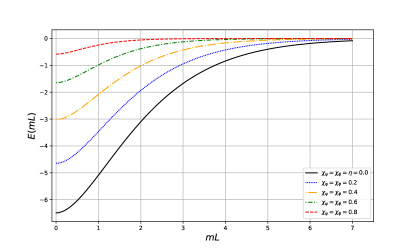
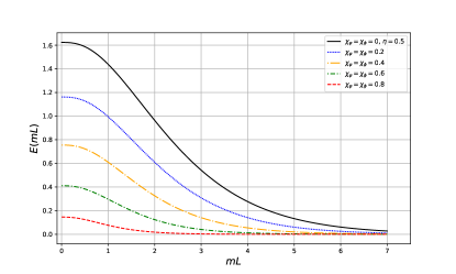
Figure 1: Graph of the dimensionless vacuum energy density $E\left(mL\right)=2\pi^{2}L^{4}\mathcal{E}_{0z}\left(mL\right)$, considering $m=\mu$ and $\chi_{\psi}=\chi_{\varphi}$.

In Fig. 1 we exhibit the dimensionless vacuum energy density $E\left(mL\right)=2\pi^{2}L^{4}\mathcal{E}_{0z}\left(mL\right)$, Eq. (33), as a function of $mL$, for several values of the parameters $\chi_{\psi}=\chi_{\varphi}$. We also consider equal masses, that is, $m=\mu$. The graph on the left shows that for a fixed value of the quasi-periodic parameter $\eta=0$, as we increase the value of the parameters $\chi_{\psi}$ and $\chi_{\varphi}$, the vacuum energy density also increases, comparing its value with the one in which the Lorentz symmetry is preserved (black solid line). The graph on the right takes the value $\eta=0.5$, showing that as we increase the values of $\chi_{\psi}$ and $\chi_{\varphi}$, the vacuum energy density decreases. Note that the vacuum energy density can be positive or negative, depending on the value of the quasi-periodic parameter $\eta$. Taking the limit $mL\rightarrow\infty$, the vacuum energy density goes to zero, as it should, since we should not expect any quantum effect in this regime.

Figure 2: Graph of the dimensionless vacuum energy density $E\left(mL\right)=2\pi^{2}L^{4}\mathcal{E}_{0z}\left(mL\right)$, considering $m=\mu$ and $\chi_{\psi}=0.2$ with some different values of $\chi_{\varphi}$.

In Fig. 2 the dimensionless vacuum energy density $E\left(mL\right)=2\pi^{2}L^{4}\mathcal{E}_{0z}\left(mL\right)$, from Eq. (33), is shown considering the value of the Lorentz violation parameter for the real field fixed, $\chi_{\psi}=0.2$, and sevreal values for the Lorentz violation parameter associated with the complex field $\chi_{\varphi}$. The graph on the left is for $\eta=0$ showing that as we increase the value of $\chi_{\varphi}$, the vacuum energy density also increases. The graph on the right considers $\eta=0.5$ and shows that as $\chi_{\varphi}$ increases, the vacuum energy density decreases. In addition, the dotted blue line which takes the values $\chi_{\psi}=0.2$ and $\chi_{\varphi}=0.4$ exhibits an interesting behaviour, starting with positive values of $E\left(mL\right)$, becoming negative and eventually going to zero again. As we can see, the vacuum energy density can be positive or negative, depending on the values of the parameters of the Lorentz violation and also, as $mL\rightarrow\infty$, the vacuum energy density goes to zero.

From the result presented in Eq. (33), we can consider the massless fields case in which we take the limit $m,\mu\rightarrow 0$. In order to obtain the vacuum energy density for the massless fields case, one can use the limit of small arguments of the Macdonald function, i.e., $K_{\mu}\left(x\right)\approx\frac{\Gamma\left(\mu\right)}{2}\left(\frac{2}{x}\right)^{\mu}$ abramowitz1965handbook . Hence, in the exact limit where the masses vanishe, we obtain,

$$\mathcal{E}_{0z}=-\left(1-\chi_{\psi}\right)^{\frac{3}{2}}\frac{\pi^{2}}{90L^{4}}-\frac{2\left(1-\chi_{\varphi}\right)^{\frac{3}{2}}}{\pi^{2}L^{4}}\sum_{j=1}^{\infty}j^{-4}\cos\left(2\pi j\eta\right),$$ (34)

where we have used the following result for the Riemann zeta function $\zeta_{\text{R}}\left(4\right)=\frac{\pi^{4}}{90}$ elizalde1995zeta ; elizalde1995ten , in the first term on the r.h.s. of Eq. (34). This term is an already known result toms1980symmetry multiplied by the factor due to the Lorentz symmetry violation, i.e., $\left(1-\chi_{\psi}\right)^{\frac{3}{2}}$. The second term can be rewritten in terms of the Bernoulli polynomials, defined as,

$$B_{2k}\left(\theta\right)=\frac{\left(-1\right)^{k-1}2\left(2k\right)!}{\left(2\pi\right)^{2k}}\sum_{n=1}^{\infty}\frac{\cos\left(2\pi n\theta\right)}{n^{2k}}.$$ (35)

Hence, one obtains the following expression for the vacuum energy density, for the massless field case,

$$\mathcal{E}_{0z}=-\left(1-\chi_{\psi}\right)^{\frac{3}{2}}\frac{\pi^{2}}{90L^{4}}+\left(1-\chi_{\varphi}\right)^{\frac{3}{2}}\frac{2\pi^{2}}{3L^{4}}\left(\eta^{4}-2\eta^{3}+\eta^{2}-\frac{1}{30}\right),$$ (36)

where the Bernoulli polynomial of fourth order, $B_{4}\left(\theta\right)=\left(\theta^{4}-2\theta^{3}+\theta^{2}-\frac{1}{30}\right)$, has been used.  As one should expect, if we take $\chi_{\psi},\chi_{\varphi}\rightarrow 0$ the first term on the r.h.s. of Eq. (36) is consistent with the resulst found in toms1980symmetry and, the second term is consistent with the resulst found in feng2014casimir (taking into accont the two components of the complex field). Therefore the modification due to the Lorentz symmetry violation is expressed by the multiplicative factors $\left(1-\chi_{\psi}\right)^{\frac{3}{2}}$, for the contribution due to the real field, and $\left(1-\chi_{\varphi}\right)^{\frac{3}{2}}$ for the contribution from the complex field. Note that the vacuum energy density can be positive or negative depending on the value of the parameter $\eta$ of the quasi-periodic condition obeyed by the components of the complex field.

Now we proceed to calculate the two-loop correction to the effective potential, in the vacuum state $\Psi=0$, which is the first order $\lambda$ correction to the vacuum energy density.

III.2 Two-loop correction

As we have mentioned in the first section of the present paper, the correction for the vacuum energy density which is first order in the coupling constants, is obtained from the two-loop Feynman graphs of the theory. Since we have more than one contribution, we evaluate the two-loop contributions from each Feynman graph separately. Hence, we write $V^{\left(2\right)}\left(\Psi\right)$ as a sum of four terms,

$$V^{\left(2\right)}\left(\Psi\right)=V_{\lambda_{\psi}}^{\left(2\right)}\left(\Psi\right)+V_{\lambda_{\varphi}}^{\left(2\right)}\left(\Psi\right)+V_{g}^{\left(2\right)}\left(\Psi\right)+V_{2\lambda_{\varphi}}^{\left(2\right)}\left(\Psi\right).$$ (37)

Each term on the r.h.s. of the above equation is associated with a term of the potential in Eq. (1), namely, $V_{\lambda_{\psi}}^{\left(2\right)}$ is the contribution from the self-interaction of the real field $\left(\frac{\lambda_{\psi}}{4!}\psi^{4}\right)$, $V_{\lambda_{\varphi}}^{\left(2\right)}$ is associated with the self-interaction of the complex field $\left(\frac{\lambda_{\varphi}}{4!}\varphi_{i}^{4}\right)$ , $V_{g}^{\left(2\right)}$ is associated with the interaction between the real and complex fields $\left(\frac{g}{2}\varphi_{i}^{2}\psi^{2}\right)$, and finally $V_{2\lambda_{\varphi}}^{\left(2\right)}$ is associated with the cross terms arising from the interaction between the components of the complex field $\left(\frac{\lambda_{\varphi}}{4!}2\varphi_{1}^{2}\varphi_{2}^{2}\right)$, which is also a self-interaction.

Figure 3: Feynman graph representing the contribution from the self-interaction potential at $\Psi=0$.

Let us first consider the contribution from the self-interaction term associated with the real field, that is, $V_{\lambda_{\psi}}^{\left(2\right)}\left(\Psi\right)$. Since we are interested in the vacuum state where $\Psi=0$, the only non-vanishing contribution comes from the graph exhibited in Fig. 3. From this Feynman graph one can write the two-loop contribution in terms of the generalized zeta function presented in Eq. (23), in the following form Aj ; porfirio2021ground ; PhysRevD.107.125019 ,

$$V_{\lambda_{\psi}}^{\left(2\right)}\left(0\right)=\frac{\lambda_{\psi}}{8}\left.\left[\frac{\zeta_{\alpha}^{R}\left(1\right)}{\Omega_{4}}\right]^{2}\right|_{\Psi=0}.$$ (38)

The zeta function $\zeta_{\alpha}^{R}\left(s\right)$, is defined as the non-divergent part of the generalized zeta function given in Eq. (23), at $s=1$ Aj ; porfirio2021ground ; PhysRevD.107.125019 , i.e.,

$$\zeta_{\alpha}^{R}\left(s\right) = \zeta_{\alpha}\left(s\right)-\frac{\Omega_{4}\left(M_{\lambda}\right)^{4-2s}}{2^{4}\pi^{2}\sqrt{1-\chi_{\psi}}}\frac{\Gamma\left(s-2\right)}{\Gamma\left(s\right)}$$ (39)

$$= \frac{\left(M_{\lambda}\right)^{2}}{2\pi^{2}\sqrt{1-\chi_{\psi}}}\sum_{n=1}^{\infty}f_{\left(1\right)}\left(\frac{nM_{\lambda}L}{\sqrt{1-\chi_{\psi}}}\right).$$

Note that the term that is being subtracted in the above expression is independent of the parameter $L$ characterizing the conditions and, as usual, it should be dropped. Explicitly, one obtains the following result for the two-loop contribution due to the self-interaction term of the real field,

$$V_{\lambda_{\psi}}^{\left(2\right)}\left(0\right)=\frac{\lambda_{\psi}m^{4}}{32\pi^{4}\left(1-\chi_{\psi}\right)}\left[\sum_{n=1}^{\infty}f_{\left(1\right)}\left(\frac{nmL}{\sqrt{\left(1-\chi_{\psi}\right)}}\right)\right]^{2},$$ (40)

which shows that the two-loop contribution is proportional to the coupling constant $\lambda_{\psi}$ as it should.

Similarly, the other contributions are written as

$$V_{\lambda_{\varphi}}^{\left(2\right)}\left(0\right)=2\frac{\lambda_{\varphi}\mu^{4}}{32\pi^{4}\left(1-\chi_{\varphi}\right)}\left[\sum_{j=1}^{\infty}\cos\left(2\pi j\eta\right)f_{\left(1\right)}\left(\frac{j\mu L}{\sqrt{\left(1-\chi_{\varphi}\right)}}\right)\right],$$ (41)

$$V_{g}^{\left(2\right)}\left(0\right)=2\frac{gm^{2}\mu^{2}}{8\pi^{4}\sqrt{\left(1-\chi_{\psi}\right)\left(1-\chi_{\varphi}\right)}}\left[\sum_{n=1}^{\infty}f_{\left(1\right)}\left(\frac{nmL}{\sqrt{\left(1-\chi_{\psi}\right)}}\right)\right]\left[\sum_{j=1}^{\infty}\cos\left(2\pi j\eta\right)f_{\left(1\right)}\left(\frac{j\mu L}{\sqrt{\left(1-\chi_{\varphi}\right)}}\right)\right],$$ (42)

$$V_{2\lambda_{\varphi}}^{\left(2\right)}\left(0\right)=\frac{\lambda_{\varphi}\mu^{4}}{48\pi^{4}\left(1-\chi_{\varphi}\right)}\left[\sum_{j=1}^{\infty}\cos\left(2\pi j\eta\right)f_{\left(1\right)}\left(\frac{j\mu L}{\sqrt{\left(1-\chi_{\varphi}\right)}}\right)\right]^{2}.$$ (43)

The contribution $V_{\lambda_{\varphi}}^{\left(2\right)}\left(0\right)$, can be read from the same graph as in Fig. 3. One constructs the zeta function $\zeta_{\beta}^{R}\left(s\right)$ from the generalized zeta function (27), subtracting the divergent part at $s=1$, which is proportional to $\lambda_{\varphi}$. The factor of $2$ is to remind that we have to account for two components of the the complex field, that is, $\varphi_{1}$ and $\varphi_{2}$ which give rise to equal contributions.

Figure 4: Feynman graph representing the contribution from the self-interaction potential at $\Psi=0$.

The next contribution $V_{g}^{\left(2\right)}\left(0\right)$, Eq. (42), is from the interaction between the fields. This correction is inferred from the graph presented in Fig. 4, and it is proportional to the coupling constant $g$. Finally, the last contribution comes from the interaction of the components of the complex field, $V_{2\lambda_{\varphi}}^{\left(2\right)}\left(0\right)$, which is also a self-interaction. This contribution is also obtained from tha graph in Fig. 4, considering the solid line as representing the propagator associated with the field $\varphi_{1}$ and the dashed one associated with the field $\varphi_{2}$. Similar to the result presented in Eq. (41), $V_{2\lambda_{\varphi}}^{\left(2\right)}\left(0\right)$ in Eq. (43) is proportional to the coupling constant $\lambda_{\varphi}$.

Collecting all results obtained in Eqs (40), (42), (41) and (43), one can write the two-loop correction to the effective potential, at the vacuum state $\Psi=0$, as

$$\Delta\mathcal{E}_{0z} = \left.V^{\left(2\right)}\left(\Psi\right)\right|_{\Psi=0}$$ (44)

$$= \frac{\lambda_{\psi}m^{4}}{32\pi^{4}\left(1-\chi_{\psi}\right)}\left[\sum_{n=1}^{\infty}f_{1}\left(\frac{nmL}{\sqrt{1-\chi_{\psi}}}\right)\right]^{2}+\frac{\lambda_{\varphi}\mu^{4}}{12\pi^{4}\left(1-\chi_{\varphi}\right)}\left[\sum_{j=1}^{\infty}\cos\left(2\pi j\eta\right)f_{1}\left(\frac{j\mu L}{\sqrt{1-\chi_{\varphi}}}\right)\right]^{2}$$

$$+\frac{gm^{2}\mu^{2}}{4\pi^{4}\sqrt{\left(1-\chi_{\psi}\right)\left(1-\chi_{\varphi}\right)}}\left[\sum_{n=1}^{\infty}f_{1}\left(\frac{nmL}{\sqrt{1-\chi_{\psi}}}\right)\right]\left[\sum_{j=1}^{\infty}\cos\left(2\pi j\eta\right)f_{1}\left(\frac{j\mu L}{\sqrt{1-\chi_{\varphi}}}\right)\right].$$

The expression above is the correction to the vacuum energy density obtained in Eq. (33). Hence, up to second order, the vacuum energy density gains correction terms proportional to each coupling constant. Each term on the r.h.s. of the above expression is affected by the Lorentz violation parameters $\chi_{\psi}$ or $\chi_{\varphi}$, in the form of a multiplicative factor as well as in the argument of the Macdonald functions. In the last term, which is proportional to the coupling constant $g$, the two Lorentz violation parameters are present since this term comes from the interaction between the two fields.

Moreover, one can consider the vacuum energy density for the massless fields case. From Eq. (44) taking $m,\mu\rightarrow 0$, it is easy to see that the correction to the vacuum energy density reads,

$$\Delta\mathcal{E}_{\mathrm{C}z}=\frac{\lambda_{\psi}\left(1-\chi_{\psi}\right)}{1152L^{4}}+\frac{\lambda_{\varphi}\left(1-\chi_{\varphi}\right)}{12L^{4}}\left(\eta^{2}-\eta+\frac{1}{6}\right)^{2}+\frac{g\sqrt{\left(1-\chi_{\psi}\right)\left(1-\chi_{\varphi}\right)}}{24L^{4}}\left(\eta^{2}-\eta+\frac{1}{6}\right).$$ (45)

In the expression above we have used the value $\zeta_{\text{R}}\left(2\right)=\frac{\pi^{2}}{6}$ elizalde1995zeta ; elizalde1995ten as well as the Bernoulli polynomials presentend in Eq. (35), with $B_{2}\left(\theta\right)=\theta^{2}-\theta+\frac{1}{6}$. This result is the vacuum energy density in the vacuum state $\Psi=0$. However, the vacuum state considered here is not the only possible state. We will see that other stable vacuum states are allowed given certain conditions PhysRevD.107.125019 .

Before we analyze the possible stable vacuum states and their stabilities, we shall investigate the generation of topological mass due the non-triviality of the spacetime, which is affected by the Lorentz symmetry violation.

III.3 Topological mass

Here we investigate the influence of the conditions studied here and the Lorentz symmetry violation in the topological mass of the real field $\psi$, i.e., the generation of the topological mass at one-loop level. Using the renormalization condition presented in Eq. (13) with the renormalized effective potential given in Eq. (32), we obtain the following expression for the topological mass of the real field,

$$m_{\text{T}}^{2}=m^{2}\left[1+\frac{\lambda_{\psi}}{4\pi^{2}\sqrt{1-\chi_{\psi}}}\sum_{n=1}^{\infty}f_{1}\left(\frac{nLm}{\sqrt{1-\chi_{\psi}}}\right)+\frac{g}{\pi^{2}\sqrt{1-\chi_{\varphi}}}\frac{\mu^{2}}{m^{2}}\sum_{j=1}^{\infty}\cos\left(2\pi j\eta\right)f_{1}\left(\frac{jL\mu}{\sqrt{1-\chi_{\varphi}}}\right)\right].$$ (46)

The Lorentz violation parameters are present in the multiplicative factors $\left(1-\chi_{\psi}\right)^{-\frac{1}{2}}$ and $\left(1-\chi_{\varphi}\right)^{-\frac{1}{2}}$, and also in the argument of the Macdonald functions.

Figure 5: Graph of the dimensionless mass squared $M^{2}\left(mL\right)=L^{2}m_{\text{T}}^{2}\left(mL\right)$, considering $m=\mu$, $\lambda_{\psi}=10^{-2}$, $g=10^{-3}$, fixed $\chi_{\psi}=0.2$ and different values of $\chi_{\varphi}$ .

In Fig. 5, it is shown the dimensionless square mass $M^{2}\left(mL\right)=L^{2}m_{\text{T}}^{2}\left(mL\right)$ as a function of $mL$, considering equal masses for the real and complex fields, $m=\mu$, and the values for the coupling constants $\lambda_{\psi}=10^{-2}$, $g=10^{-3}$, with fixed $\chi_{\psi}=0.2$ and different values of $\chi_{\varphi}$. The graph on the left takes the value $\eta=0$ for the quasi-periodic parameter and shows that as we increase $\chi_{\varphi}$ the topological mass decreases, while the graph on the right takes the value $\eta=0.5$ and shows the opposite behavior.

Since the expression (46) for the topological mass $m_{\text{T}}^{2}$ does not present any divergence, one can consider the massless field case, i.e., the limit $m,\mu\rightarrow 0$, and using the same approximation as before, that is, $K_{\mu}\left(x\right)\approx\frac{\Gamma\left(\mu\right)}{2}\left(\frac{2}{x}\right)^{\mu}$ abramowitz1965handbook , we find the topological mass for the massless field case as,

$$m_{\text{T}}^{2}=\sqrt{1-\chi_{\psi}}\frac{\lambda_{\psi}}{24L^{2}}+\sqrt{1-\chi_{\varphi}}\frac{g}{L^{2}}\left(\eta^{2}-\eta+\frac{1}{6}\right),$$ (47)

where we have used the result for the Riemann zeta function $\zeta_{\text{R}}\left(2\right)=\frac{\pi^{2}}{6}$ elizalde1995zeta ; elizalde1995ten and also the Bernoulli polynomials presentend in Eq. (35), together with the representation $B_{2}\left(\theta\right)=\theta^{2}-\theta+\frac{1}{6}$. As one can see, the mass correction at one-loop level comes from the self-interaction term, which is proportional to $\lambda_{\psi}$, and also from the interaction between the fields, which is proportional to the coupling constant $g$. Besides, the topological mass has been affected by the Lorentz symmetry violation, which appears as the multiplicative factors $\sqrt{1-\chi_{\psi}}$ and $\sqrt{1-\chi_{\varphi}}$ in the contributions from the real and complex fields, respectively.

The topological mass presented in Eq. (47) can be positive or negative, depending on the value of the coupling constants $\lambda_{\psi}$ and $g$, and also on the value of the phase angle, $\eta$, associated with the quasi-periodic condition imposed on the components of the complex field. If the conditions are so that the topological mass is negative, this in principle implicates vacuum instability.

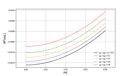
Figure 6: Graph of the dimensionless mass squared $M^{2}\left(mL\right)=L^{2}m_{\text{T}}^{2}\left(mL\right)$, considering $m=\mu$, $\lambda_{\psi}=10^{-3}$, $g=10^{-2}$, and equal values for the Lorentz violation parameters $\chi_{\psi}=\chi_{\varphi}$ .

The graph exhibited in Fig. 6 shows that the dimensionless squared mass $M^{2}\left(mL\right)$ can be negative, for some values of the parameters. The graph takes the values $\lambda_{\psi}=10^{-3}$, $g=10^{-2}$ for the coupling constants, $\eta=0.5$ for the quasi-periodic parameter and equal values for the Lorentz violation parameters, that is, $\chi_{\psi}=\chi_{\varphi}$.

In the next section we shall analyze the possible vacuum states and their corresponding stability conditions, which depends on the values of the coupling constants and also on the Lorentz violation parameters.

III.4 Vacuum stability

In this section we investigate the possible vacuum states and the stability for the theory described by the action presented in Eq. (1). However, for simplicity, we consider the massless field case, i.e., $m,\mu\rightarrow 0$. Hence, for a real field interacting with a complex field, under periodic and quasi-periodic conditions, respectively, and with the Lorentz symmetry violation in the $z$-direction, the nonrenormalized effective potential is,

$$V_{\mathrm{eff}}\left(\Psi\right)_{z}=\frac{\lambda_{\psi}+C}{4!}\Psi^{4}+\frac{\lambda_{\psi}^{2}\Psi^{4}}{2^{8}\pi^{2}\sqrt{1-\chi_{\psi}}}\left[\ln\left(\frac{\frac{1}{2}\lambda_{\psi}\Psi^{2}}{\nu^{2}}\right)-\frac{3}{2}\right]+\frac{g^{2}\Psi^{4}}{2^{5}\pi^{2}\sqrt{1-\chi_{\varphi}}}\left[\ln\left(\frac{g\Psi^{2}}{\nu^{2}}\right)-\frac{3}{2}\right]$$

$$-\frac{\lambda_{\psi}^{2}\Psi^{4}}{2^{3}\pi^{2}\sqrt{1-\chi_{\psi}}}\sum_{n=1}^{\infty}f_{2}\left(\frac{n\sqrt{\frac{\lambda_{\psi}}{2}}\Psi L}{\sqrt{1-\chi_{\psi}}}\right)-\frac{g^{2}\Psi^{4}}{\pi^{2}\sqrt{1-\chi_{\varphi}}}\sum_{j=1}^{\infty}\cos\left(2\pi j\eta\right)f_{2}\left(\frac{j\sqrt{g}\Psi L}{\sqrt{1-\chi_{\varphi}}}\right).$$ (48)

Note that in the case under consideration we only need one constant of renormalization, namely $C$. The renormalization condition which gives the explicit form of $C$ is presented in Eq. (12), yielding

$$C=\frac{3\lambda_{\psi}^{2}}{32\pi^{2}\sqrt{1-\chi_{\psi}}}\left[\ln\left(\frac{2\nu^{2}}{\lambda_{\psi}M^{2}}\right)-\frac{8}{3}\right]+\frac{3g^{2}}{4\pi^{2}\sqrt{1-\chi_{\varphi}}}\left[\ln\left(\frac{\nu^{2}}{gM^{2}}\right)-\frac{8}{3}\right],$$ (49)

where $M$ is a parameter which has dimension of mass. Substituting the constant $C$ above, on the effective potential (48), one finds the renormalized effective potential for the massless field case, i.e.,

$$V_{\text{{eff}}}^{R}\left(\Psi\right)_{z}=\frac{\lambda_{\psi}}{4!}\Psi^{4}+\frac{\Psi^{4}}{32\pi^{2}}\ln\left(\frac{\Psi^{2}}{M^{2}}\right)\left(\frac{\lambda_{\psi}^{2}}{8\sqrt{1-\chi_{\psi}}}+\frac{g^{2}}{\sqrt{1-\chi_{\varphi}}}\right)-\frac{25g^{2}\Psi^{4}}{192\pi^{2}}\left(\frac{\lambda_{\psi}^{2}}{8\sqrt{1-\chi_{\psi}}}+\frac{g^{2}}{\sqrt{1-\chi_{\varphi}}}\right)$$

$$-\frac{\lambda_{\psi}^{2}\Psi^{4}}{8\pi^{2}\sqrt{1-\chi_{\psi}}}\sum_{n=1}^{\infty}f_{2}\left(\frac{n\sqrt{\frac{1}{2}\lambda_{\psi}}\Psi L}{\sqrt{1-\chi_{\psi}}}\right)-\frac{g^{2}\Psi^{4}}{\pi^{2}\sqrt{1-\chi_{\varphi}}}\sum_{j=1}^{\infty}\cos\left(2\pi j\eta\right)f_{2}\left(\frac{j\sqrt{g}\Psi L}{\sqrt{1-\chi_{\varphi}}}\right).$$ (50)

In order to investigate the vacuum state, up to first order in the coupling constants $\lambda_{\psi}$ and $g$, we expand the renormalized effective potential given in Eq. (50) in powers of $\lambda_{\psi}$ and $g$ toms1980interacting ; PhysRevD.107.125019 , up to first order. The result is given by

$$V_{\mathrm{eff}}^{R}\left(\Psi\right)_{z;\lambda_{\psi},g} = -\frac{\left(1-\chi_{\psi}\right)^{\frac{3}{2}}\pi^{2}}{90L^{4}}+\frac{2\left(1-\chi_{\varphi}\right)^{\frac{3}{2}}\pi^{2}}{3L^{4}}B_{4}\left(\eta\right)+\frac{\lambda_{\psi}}{4!}\Psi^{4}$$ (51)

$$+\frac{\Psi^{2}}{48L^{2}}\left[\sqrt{1-\chi_{\psi}}\lambda_{\psi}+\sqrt{1-\chi_{\varphi}}24gB_{2}\left(\eta\right)\right],$$

where $B_{4}\left(\eta\right)$ and $B_{2}\left(\eta\right)$ are the fourth and second order Bernoulli polynominals defined in Eq. (35), respectively. The minima of the potential that correspond to the possible vacuum states are given by

$$\Psi=0,\qquad\qquad\Psi_{\pm}=\pm\frac{1}{2L}\sqrt{-\left[\sqrt{1-\chi_{\psi}}+\sqrt{1-\chi_{\varphi}}24B_{2}\left(\eta\right)\frac{g}{\lambda_{\psi}}\right]}.$$ (52)

The state $\Psi_{0}$ was considered in the previous section and $\Psi_{\pm}$ are the other possible vacuum states. Note that the Lorentz violation parameters direct influence the vacuum states $\Psi_{\pm}$ with the factors $\sqrt{1-\chi_{\psi}}$ and $\sqrt{1-\chi_{\varphi}}$. Now we have to analyze which vacuum state is a physical one, that is, which one is stable. The stability is investigated from the second derivative of the expanded potential in Eq. (51), that is,

$$\frac{d^{2}}{d\Psi^{2}}V_{\mathrm{eff}}^{R}\left(\Psi\right)_{z;\lambda_{\psi},g}=\frac{\lambda_{\psi}}{2}\Psi^{2}+\frac{1}{24L^{2}}\left[\sqrt{1-\chi_{\psi}}\lambda_{\psi}+\sqrt{1-\chi_{\varphi}}24gB_{2}\left(\eta\right)\right].$$ (53)

For the vacuum state to be stable, the second derivative of the potential, evaluated at this state must be greater than zero. This of course depends on the coupling constants and also on the Lorentz symmetry violation parameters.

We start with the zero vacuum state, that is, $\Psi=0$ which was the case considered in the previous sections. In this case, from Eq. (53), one sees that the vacuum state $\Psi=0$ is stable if the following condition is satisfied,

$$\lambda_{\psi}>-24R_{\varphi\psi}^{z}gB_{2}\left(\eta\right),$$ (54)

where we have defined the quantity,

$$R_{\varphi\psi}^{z}=\sqrt{\frac{1-\chi_{\varphi}}{1-\chi_{\psi}}}.$$ (55)

Therefore the Lorentz violation affects the vacuum stability via factor $R_{\varphi\psi}^{z}$. However, if the parameters $\chi_{\psi}$ and $\chi_{\varphi}$ are equal $\chi_{\psi}=\chi_{\psi}$, then $R_{\varphi\psi}^{z}=1$ and we recover the result presented in PhysRevD.107.125019 . The parameter $\eta$ which is associated with the condition on the complex field, and the coupling constants, $\lambda_{\psi}$ and $g$, also influence in the vacuum stability. Furthermore, if the coupling constants, $\lambda_{\psi}$ and $g$, are taken to be positive along with $R_{\varphi\psi}^{z}$ and $B_{2}\left(\eta\right)$, then the condition (54) is automatically satisfied. However, if $B_{2}\left(\eta\right)$ is negative, the condition (54) may be violated. Using the explicit form of the Bernoulli polynomial, that is, $B_{2}\left(\eta\right)=\eta^{2}-\eta+\frac{1}{6}$, one finds that it is negative for the values of $\eta$ in the range,

$$\frac{1}{2}-\frac{\sqrt{3}}{6}<\eta<\frac{1}{2}+\frac{\sqrt{3}}{6}.$$ (56)

For $\eta$ inside the above interval, we have to apply condition (54) in order to obtain the allowed values for the coupling constants such that the vacuum state $\Psi=0$ is stable. For instance, let us consider the value $\eta=1/2$, i.e., the components of the complex field, $\varphi_{i}$, are twisted. Then, the condition of stability written in Eq. (54), becomes,

$$\lambda_{\psi}>2R_{\varphi\psi}^{z}g.$$ (57)

The condition above is in agreement with the one found in PhysRevD.107.125019 and also toms1980interacting if there was no Lorentz symmetry violation or the parameters $\chi_{\psi}$ and $\chi_{\varphi}$ are equal. Since the model includes the Lorentz symmetry violation and allows different values for the parameters, we have to consider the quantity $R_{\varphi\psi}^{z}$. The topological mass, for this case, takes the following form,

$$m_{\text{T}}^{2}=\frac{\sqrt{1-\chi_{\psi}}\lambda_{\psi}-2\sqrt{1-\chi_{\varphi}}g}{24L^{2}},$$ (58)

which agrees with the result obtained in Eq. (47) with $\eta=1/2$. Note also that if the interaction between the fields is not present, that is, $g=0$, and also there is no Lorentz symmetry violation, then it reproduces previous known results Ford:1978ku .

Next we consider the other vacuum states, i.e., $\Psi=\Psi_{\pm}$ from Eq. (52). In this case, the second derivative of the effective potential, Eq. (53), give rise to the following condition:

$$\lambda_{\psi}<-24R_{\varphi\psi}^{z}gB_{2}\left(\eta\right).$$ (59)

Note that the states $\Psi_{\pm}$ depends on the Lorentz symmetry violation parameters $\chi_{\psi}$. However, the stability condition is affected if and only if the parameters are different, $\chi_{\psi}\neq\chi_{\varphi}$. Since we are taking the coupling constants as positive numbers, then $B_{2}\left(\eta\right)<0$ which gives the same interval as the Eq. (56) for the parameter $\eta$. From this observation, one can conclude that the possible values of the parameter $\eta$, that makes possible to $\Psi_{\pm}$ be a stable vacuum state are within the interval given in Eq. (56). Considering again the value $\eta=1/2$, we obtain the stability condition as,

$$\lambda_{\psi}<2R_{\varphi\psi}^{z}g.$$ (60)

Furthermore the topological mass now reads,

$$m_{\text{T}}^{2}=\frac{2g\sqrt{1-\chi_{\varphi}}-\lambda_{\psi}\sqrt{1-\chi_{\psi}}}{12L^{2}}.$$ (61)

Since we are taken a different vacuum state from $\Psi=0$, we expect that the topological mass (61) differ from the one given in Eq. (58), which is the case here.

The vacuum energy density is also considered in the study of the vacuum stability. Considering the case of the vacuum state being $\Psi=0$ and in addition, the value $\eta=1/2$ for the parameter of the quasi-periodic condition, one obtains the vacuum energy density as being the same as the one presented in Eq. (36) with $\eta=1/2$. However, considering that the vacuum state is $\Psi=\Psi_{\pm}$, (52), one can substitute this state in the expanded effective potential given in Eq (51), to obtain the following expressions for the vacuum energy density,

$$V_{\mathrm{eff}}^{R}\left(\Psi_{\pm}\right)_{z;\lambda_{\psi},g}\simeq-\frac{\left(1-\chi_{\psi}\right)^{\frac{3}{2}}\pi^{2}}{90L^{4}}+\frac{2\left(1-\chi_{\varphi}\right)^{\frac{3}{2}}\pi^{2}}{3L^{4}}B_{4}\left(\eta\right)-\frac{1}{384\lambda_{\psi}L^{4}}\left[\sqrt{1-\chi_{\psi}}\lambda_{\psi}+\sqrt{1-\chi_{\varphi}}24gB_{2}\left(\eta\right)\right]^{2}.$$ (62)

Note that the first two terms on the r.h.s. of Eq. (62) are in agreement with the vacuum energy density presented in Eq. (36). However, the last term presents a dependence on the coupling constants $\lambda_{\psi}$ and $g$, which does not appears in the case where the vacuum state is $\Psi=0$. It is important to point out that the expression above is only an approximation, since we are taking the expansion of the effective potential presented in Eq. (51).

From Eqs. (54) and (59), we conclude that the stability of the vacuum state is determined by the values of the Lorentz violation parameters $\chi_{\psi}$ and $\chi_{\varphi}$, coupling constants $\lambda_{\psi}$ and $g$, and also depends on the value of the parameter $\eta$ of the condition for the complex field. However it shows no dependence on the parameter $L$ PhysRevD.107.125019 .

To end this section let us discuss the effect of the Lorentz violation scenario in which we are considering in the $\tau$, $x$ and $y$ directions. In the temporal direction, the effect of the Lorentz violation on the vacuum energy density and topological mass of each field is only by means of a global multiplicative factor $\sqrt{1+\chi}$ in the denominator. In contrast, in the spatial directions $x$ and $y$, the effect of the Lorentz violation is only by means of a global multiplicative factor $\sqrt{1-\chi}$ in the numerator. In these cases, the vacuum energy density and topological mass are trivially attenuated by the mentioned factors, since $\chi$ is to be considered smaller than unit (see Refs. cruz2020casimir ; Aj ). Therefore, the Lorentz violation effect is nontrivial when we consider the same direction as the one along which the condition is imposed.

IV Concluding remarks

The vacuum energy density, its loop correction and the generation of the topological mass was investigated for a system consisting of a real field, interacting with a complex one via quartic interaction. Besides, the self-interaction potential of each field was included. The whole system is considered in a scenario in which the CPT-even aether-type violation of Lorentz symmetry takes place. Both vacuum energy density and topological mass arise from the nontrivial topology of the spacetime, induced by periodic and quasi-periodic conditions imposed on the fields. The real field is subject to periodic condition while the complex is assumed to obey the quasi-periodic condition.

Considering that the CPT-even aether-type violation of Lorentz symmetry occurs in the $z$-direction, the vacuum energy density was obtained in Eq. (33), for massive fields, and in Eq. (36), for the massless fields case. These results shows the dependence of the vacuum energy density on the lenght $L$ and also in the parameters of the Lorentz symmetry violation $\chi_{\psi}$ and $\chi_{\varphi}$ of the real and complex fields, respectively. The two-loop correction contributions to the vacuum energy density, considering both massive and massless fields cases, have been presented, respectively, in Eqs. (44) and (45), which turn out to be proportional to the coupling constants $\lambda_{\psi}$, $\lambda_{\varphi}$ and $g$. Also, the topological mass for this system was obtained in Eqs. (46) and Eq. (47), for the massive and massless cases, respectively. Furthermore, it was investigated the possible vacuum states and their corresponding stability conditions. The possible vacuum states have been presented in Eq. (52) and the corresponding stability for each state is written in Eqs. (54) and (59), which exhibit a dependence on the values of the coupling constantes $\lambda_{\psi}$, $\lambda_{\varphi}$, $g$ and on the parameter $\eta$ of the quasi-periodic condition, it also depends on the parameters of the Lorentz symmetry violation $\chi_{\psi}$ and $\chi_{\varphi}$. It is shown that although the possible vacuum states depend on the parameters $\chi_{\psi}$ and $\chi_{\varphi}$, if $\chi_{\psi}$ and $\chi_{\varphi}$ are equal, the stability condition does not depend on theses parameters and we recover the case in which there is no Lorentz symmetry violation PhysRevD.107.125019 , for the stability condition. Also, the vacuum stability does not depend on the periodic parameter $L$.

We have also discussed the rather trivial effect of the Lorentz symmetry violation on the vacuum energy density and topological mass in the $\tau$, $x$ and $y$ directions. As we have pointed out, this happens by means of global multiplicative factors, that is, $\sqrt{1+\chi}$ in the denominator in the case of temporal direction, and $\sqrt{1-\chi}$ in the numerator in the case of $x$ and $y$ directions.

- (1) H. B. Casimir, On the attraction between two perfectly conducting plates, in Proc. Kon. Ned. Akad. Wet., vol. 51, p. 793, 1948.
- (2) M. J. Sparnaay, Measurements of attractive forces between flat plates, Physica 24 (1958) 751–764.
- (3) G. Bressi, G. Carugno, R. Onofrio, and G. Ruoso, Measurement of the Casimir force between parallel metallic surfaces, Phys. Rev. Lett. 88 (2002) 041804, [quant-ph/0203002].
- (4) W. J. Kim, M. Brown-Hayes, D. A. R. Dalvit, J. H. Brownell, and R. Onofrio, Anomalies in electrostatic calibrations for the measurement of the casimir force in a sphere-plane geometry, Phys. Rev. A 78 (Aug, 2008) 020101.
- (5) S. K. Lamoreaux, Demonstration of the casimir force in the 0.6 to range, Phys. Rev. Lett. 78 (Jan, 1997) 5–8.
- (6) S. Lamoreaux, Erratum: Demonstration of the casimir force in the 0.6 to 6 m range [phys. rev. lett. 78, 5 (1997)], Physical Review Letters 81 (1998), no. 24 5475.
- (7) U. Mohideen and A. Roy, Precision measurement of the Casimir force from 0.1 to 0.9 micrometers, Phys. Rev. Lett. 81 (1998) 4549–4552, [physics/9805038].
- (8) V. M. Mostepanenko, New experimental results on the casimir effect, Brazilian Journal of Physics 30 (2000), no. 2 309–315.
- (9) Q. Wei, D. A. R. Dalvit, F. C. Lombardo, F. D. Mazzitelli, and R. Onofrio, Results from electrostatic calibrations for measuring the casimir force in the cylinder-plane geometry, Phys. Rev. A 81 (May, 2010) 052115.
- (10) M. Bordag, G. L. Klimchitskaya, U. Mohideen, and V. M. Mostepanenko, Advances in the Casimir effect, vol. 145. OUP Oxford, 2009.
- (11) K. A. Milton, The Casimir effect: physical manifestations of zero-point energy. World Scientific, 2001.
- (12) V. Mostepanenko, N. Trunov, and R. Znajek, The Casimir Effect and Its Applications. Oxford science publications. Clarendon Press, 1997.
- (13) R. Saghian, M. A. Valuyan, A. Seyedzahedi, and S. S. Gousheh, Casimir Energy For a Massive Dirac Field in One Spatial Dimension: A Direct Approach, Int. J. Mod. Phys. A 27 (2012) 1250038, [arXiv:1204.3181].
- (14) A. A. Saharian and E. R. Bezerra de Mello, Spinor Casimir densities for a spherical shell in the global monopole space-time, J. Phys. A 37 (2004) 3543, [hep-th/0307261].
- (15) A. Flachi, M. Nitta, S. Takada, and R. Yoshii, Sign flip in the casimir force for interacting fermion systems, Physical review letters 119 (2017), no. 3 031601.
- (16) G. Aleixo and H. F. S. Mota, Thermal Casimir effect for the scalar field in flat spacetime under a helix boundary condition, Phys. Rev. D 104 (2021), no. 4 045012, [arXiv:2105.0822].
- (17) A. Romeo and A. A. Saharian, Casimir effect for scalar fields under Robin boundary conditions on plates, J. Phys. A 35 (2002) 1297–1320, [hep-th/0007242].
- (18) R. V. Maluf, D. M. Dantas, and C. A. S. Almeida, The Casimir effect for the scalar and Elko fields in a Lifshitz-like field theory, Eur. Phys. J. C 80 (2020), no. 5 442, [arXiv:1905.0482].
- (19) C. A. Escobar, A. Martín-Ruiz, R. Linares, and J. M. Silva, A coherent state approach to the Casimir effect for a massive scalar field in a noncommutative spacetime, Annals Phys. 460 (2024) 169570.
- (20) V. A. Kosteleckỳ and S. Samuel, Spontaneous breaking of lorentz symmetry in string theory, Physical Review D 39 (1989), no. 2 683.
- (21) P. Hořava, Quantum gravity at a lifshitz point, Physical Review D 79 (2009), no. 8 084008.
- (22) A. J. D. Farias Junior and H. F. Mota Santana, Loop correction to the scalar Casimir energy density and generation of topological mass due to a helix boundary condition in a scenario with Lorentz violation, Int. J. Mod. Phys. D 31 (2022), no. 16 2250126, [arXiv:2204.0940].
- (23) A. F. Santos and F. C. Khanna, Corrections Due to Lorentz Violation, Finite Temperature, and Magnetic Field for the Casimir Effect of a Massive Scalar Field, Int. J. Theor. Phys. 61 (2022), no. 4 96.
- (24) M. B. Cruz, E. R. Bezerra de Mello, and H. F. Santana Mota, Casimir energy and topological mass for a massive scalar field with Lorentz violation, Phys. Rev. D 102 (2020), no. 4 045006, [arXiv:2005.0951].
- (25) R. A. Dantas, H. F. S. Mota, and E. R. Bezerra de Mello, Bosonic casimir effect in an aether-like lorentz-violating scenario with higher order derivatives, Universe 9 (2023), no. 5 241.
- (26) D. Colladay and V. A. Kostelecký, violation and the standard model, Phys. Rev. D 55 (Jun, 1997) 6760–6774.
- (27) D. Colladay and V. A. Kostelecký, Lorentz-violating extension of the standard model, Phys. Rev. D 58 (Oct, 1998) 116002.
- (28) A. Anisimov, T. Banks, M. Dine, and M. Graesser, Comments on noncommutative phenomenology, Phys. Rev. D 65 (2002) 085032, [hep-ph/0106356].
- (29) C. E. Carlson, C. D. Carone, and R. F. Lebed, Bounding noncommutative qcd, Physics Letters B 518 (2001), no. 1-2 201–206.
- (30) J. L. Hewett, F. J. Petriello, and T. G. Rizzo, Signals for noncommutative interactions at linear colliders, Physical Review D 64 (2001), no. 7 075012.
- (31) O. Bertolami and L. Guisado, Noncommutative field theory and violation of translation invariance, Journal of High Energy Physics 2003 (2003), no. 12 013.
- (32) V. A. Kosteleckỳ, R. Lehnert, and M. J. Perry, Spacetime-varying couplings and lorentz violation, Physical Review D 68 (2003), no. 12 123511.
- (33) L. Anchordoqui and H. Goldberg, Time variation of the fine structure constant driven by quintessence, Physical Review D 68 (2003), no. 8 083513.
- (34) O. Bertolami, Lorentz invariance and the cosmological constant, Classical and Quantum Gravity 14 (1997), no. 10 2785.
- (35) J. Alfaro, H. A. Morales-Tecotl, and L. F. Urrutia, Quantum gravity corrections to neutrino propagation, Physical Review Letters 84 (2000), no. 11 2318.
- (36) J. Alfaro, H. A. Morales-Tecotl, and L. F. Urrutia, Loop quantum gravity and light propagation, Physical Review D 65 (2002), no. 10 103509.
- (37) R. K. Obousy and G. Cleaver, Radius Destabilization in Five Dimensional Orbifolds from Lorentz Violating Fields, Mod. Phys. Lett. A 24 (2009) 1495–1506, [arXiv:0805.0019].
- (38) R. Obousy and G. Cleaver, Casimir Energy and Brane Stability, J. Geom. Phys. 61 (2011) 577–588, [arXiv:0810.1096].
- (39) A. Martín-Ruiz and C. A. Escobar, Casimir effect between ponderable media as modeled by the standard model extension, Phys. Rev. D 94 (Oct, 2016) 076010.
- (40) A. Martín-Ruiz and C. A. Escobar, Local effects of the quantum vacuum in lorentz-violating electrodynamics, Phys. Rev. D 95 (Feb, 2017) 036011.
- (41) C. A. Escobar, L. Medel, and A. Martín-Ruiz, Casimir effect in lorentz-violating scalar field theory: A local approach, Phys. Rev. D 101 (May, 2020) 095011.
- (42) D. J. Toms, Symmetry Breaking and Mass Generation by Space-time Topology, Phys. Rev. D 21 (1980) 2805.
- (43) P. J. Porfírio, H. F. Santana Mota, and G. Q. Garcia, Ground state energy and topological mass in spacetimes with nontrivial topology, Int. J. Mod. Phys. D 30 (2021), no. 08 2150056, [arXiv:1908.0051].
- (44) D. J. Toms, Interacting Twisted and Untwisted Scalar Fields in a Nonsimply Connected Space-time, Annals Phys. 129 (1980) 334.
- (45) Z.-L. Wang and W.-Y. Ai, Particle production from oscillating scalar backgrounds in an FLRW universe, arXiv:2202.0821.
- (46) D. Grüneberg and H. W. Diehl, Thermodynamic casimir effects involving interacting field theories with zero modes, Phys. Rev. B 77 (Mar, 2008) 115409.
- (47) M. Cruz, E. Bezerra de Mello, and A. Petrov, Thermal corrections to the casimir energy in a lorentz-breaking scalar field theory, Modern Physics Letters A 33 (05, 2018) 37.
- (48) A. Erdas, Thermal effects on the Casimir energy of a Lorentz-violating scalar in magnetic field, Int. J. Mod. Phys. A 36 (2021), no. 20 2150155, [arXiv:2103.1282].
- (49) A. J. D. F. Junior and H. F. S. Mota, Casimir effect, loop corrections, and topological mass generation for interacting real and complex scalar fields in minkowski spacetime with different conditions, Phys. Rev. D 107 (Jun, 2023) 125019.
- (50) S. M. Carroll and H. Tam, Aether compactification, Physical Review D 78 (2008), no. 4 044047.
- (51) M. Gomes, J. Nascimento, A. Y. Petrov, and A. Da Silva, Aetherlike lorentz-breaking actions, Physical Review D 81 (2010), no. 4 045018.
- (52) A. Chatrabhuti, P. Patcharamaneepakorn, and P. Wongjun, Æther field, casimir energy and stabilization of the extra dimension, Journal of High Energy Physics 2009 (2009), no. 08 019.
- (53) C.-J. Feng, X.-Z. Li, and X.-H. Zhai, Casimir Effect under Quasi-Periodic Boundary Condition Inspired by Nanotubes, Mod. Phys. Lett. A 29 (2014) 1450004, [arXiv:1312.1790].
- (54) R. Jackiw, Functional evaluation of the effective potential, Phys. Rev. D 9 (1974) 1686.
- (55) R. L. Jaffe, The Casimir effect and the quantum vacuum, Phys. Rev. D 72 (2005) 021301, [hep-th/0503158].
- (56) H. E. Haber, O. Ogreid, P. Osland, and M. N. Rebelo, Implications of symmetries in the scalar sector, in Journal of Physics: Conference Series, vol. 1586, p. 012048, IOP Publishing, 2020.
- (57) W. Greiner and J. Reinhardt, Field quantization. Springer Science & Business Media, 2013.
- (58) L. H. Ryder, Quantum field theory. Cambridge university press, 1996.
- (59) S. W. Hawking, Zeta Function Regularization of Path Integrals in Curved Space-Time, Commun. Math. Phys. 55 (1977) 133.
- (60) S. R. Coleman and E. J. Weinberg, Radiative Corrections as the Origin of Spontaneous Symmetry Breaking, Phys. Rev. D 7 (1973) 1888–1910.
- (61) M. Abramowitz and I. A. Stegun, Handbook of mathematical functions dover publications, New York 361 (1965).
- (62) E. Elizalde, S. D. Odintsov, A. Romeo, A. A. Bytsenko, and S. Zerbini, Zeta regularization techniques with applications. World Scientific Publishing, Singapore, 1994.
- (63) E. Elizalde, Ten physical applications of spectral zeta functions, vol. 35. 1995.
- (64) L. H. Ford and T. Yoshimura, Mass Generation by Selfinteraction in Nonminkowskian Space-Times, Phys. Lett. A 70 (1979) 89–91.