MagicDrive3D: Controllable 3D Generation for Any-View Rendering in Street Scenes

Abstract

While controllable generative models for images and videos have achieved remarkable success, high-quality models for 3D scenes, particularly in unbounded scenarios like autonomous driving, remain underdeveloped due to high data acquisition costs. In this paper, we introduce MagicDrive3D, a novel pipeline for controllable 3D street scene generation that supports multi-condition control, including BEV maps, 3D objects, and text descriptions. Unlike previous methods that reconstruct before training the generative models, MagicDrive3D first trains a video generation model and then reconstructs from the generated data. This innovative approach enables easily controllable generation and static scene acquisition, resulting in high-quality scene reconstruction. To address the minor errors in generated content, we propose deformable Gaussian splatting with monocular depth initialization and appearance modeling to manage exposure discrepancies across viewpoints. Validated on the nuScenes dataset, MagicDrive3D generates diverse, high-quality 3D driving scenes that support any-view rendering and enhance downstream tasks like BEV segmentation. Our results demonstrate the framework’s superior performance, showcasing its transformative potential for autonomous driving simulation and beyond.

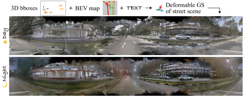
Figure 1: Rendered panorama of the street scene generated from MagicDrive3D. With conditional controls from 3D bounding boxes of objects, BEV road map, and text descriptions (e.g., weather), MagicDrive3D generates complex open-world 3D scenes represented by deformable Gaussians.

1 Introduction

With the advancement of generative models, particularly diffusion models [10, 11, 25, 21], there has been increasing interest in generating 3D assets [19, 28, 2]. While a significant amount of work has focused on object-centric generation [19, 27], generating open-ended 3D scenes remains relatively unexplored. This gap is even more critical because many downstream applications, such as Virtual Reality (VR) and autonomous driving simulation, require controllable generation of 3D street scenes, which is an open challenge.

3D-aware view synthesis methods can be broadly categorized into two approaches: geometry-free view synthesis and geometry-focused scene generation [22]. Geometry-free methods directly generate 2D images [5] or videos [9, 32, 30] based on camera parameters, excelling in photo-realistic image generation. However, they often lack sufficient geometric consistency, limiting their ability to extend to viewpoints beyond the dataset [9, 32, 30]. On the other hand, geometry-focused methods (e.g., GAUDI [2] and NF-LDM [13]) generate 3D representations (e.g., NeRF [18] or voxel grids) from latent inputs, supporting multi-view rendering. Despite their broader applicability, these methods require expensive data collection, necessitating static scenes and consistent sensor properties like exposure and white balance. Street view datasets, such as nuScenes [4], often fail to meet these requirements, making it extremely challenging to train geometry-focused 3D street scene generation models using such datasets.

Recognizing the advancements in controllable generation by geometry-free view synthesis methods [5, 9], it is potential to use them as data engines. Their controllability and photo-realism could address the challenges faced by geometry-focused methods. However, the limited 3D consistency in synthetic views from geometry-free methods, such as temporal inconsistency among frames and deformation of objects, poses crucial issues for integrating two kinds of methods into a unified framework.

To address these challenges, we propose MagicDrive3D, a novel framework that combines geometry-free view synthesis and geometry-focused reconstruction for controllable 3D street scene generation. As illustrated in Figure 2, our approach begins with training a multi-view video generation model to synthesize multiple views of a static scene. This model is configured using controls from object boxes, road maps, text prompts, and camera poses. To enhance inter-frame 3D consistency, we incorporate coordinate embeddings that represent the relative transformation between LiDAR coordinates for accurate control of frame positions. Next, we improve the reconstruction quality of generated views by enhancing 3D Gaussian splatting from the perspectives of prior knowledge, modeling, and loss functions. Given the limited overlap between different camera views [33], we adopt a monocular depth prior and propose a dedicated algorithm for alignment in sparse-view settings. Additionally, we introduce deformable Gaussian splatting and appearance embedding maps to handle local dynamics and exposure discrepancies, respectively.

Demonstrated by extensive experiments, our MagicDrive3D framework excels in generating highly realistic street scenes that align with road maps, 3D bounding boxes, and text descriptions, as exemplified in Figure 1. We show that the generated camera views can augment training for Bird’s Eye View (BEV) segmentation tasks, providing comprehensive controls for scene generation and enabling the creation of novel street scenes for autonomous driving simulation. Notably, MagicDrive3D is the first to achieve controllable 3D street scene generation using a training dataset with only six camera perspectives, as seen in the nuScenes dataset [4].

We summarize our contributions as follows:

• We propose MagicDrive3D, the first framework to effectively integrate both geometry-free and geometry-focused view synthesis for controllable 3D street scene generation. MagicDrive3D generates realistic 3D street scenes that support rendering from any camera view according to various control signals.

• We introduce a relative pose embedding technique to generate videos with improved 3D consistency. Additionally, we enhance the reconstruction quality with tailored techniques, including deformable Gaussian splatting, to handle local dynamics and exposure discrepancies in the generated videos.

• Through extensive experiments, we demonstrate that MagicDrive3D generates high-quality street scenes with multi-dimensional controllability. Our results also show that synthetic data improves 3D perception tasks, highlighting the practical benefits of our approach.

2 Related Work

3D Scene Generation. Numerous 3D-aware generative models can synthesize images with explicit camera pose control [36, 22] and potentially other scene properties [26], but only a few scale for open-ended 3D scene generation. GSN [7] and GAUDI [2], representative of models generating indoor scenes, utilize NeRF [18] with latent code input for “floorplan” or tri-plane feature. Their reliance on datasets covering different camera poses is incompatible with typical driving datasets where camera configuration remains constant. NF-LDM [13] develops a hierarchical latent diffusion model for scene feature voxel grid generation. However, their representation and complex modeling hinder fine detail generation.

Contrary to previous works focusing on scene generation using explicit geometry, often requiring substantial data not suitable for typical street view datasets (e.g., nuScenes [4]) as discussed in Section 1, we propose merging geometry-free view synthesis with geometry-focused scene representations for controllable street scene creation. Methodologically, LucidDreamer [6] is most similar to our approach, although it relies on a text-controlled image generation model, which cannot qualify as a view synthesis model. In contrast, our video generation model is 3D-aware. Besides, we propose several improvements over 3DGS for better scene generation quality.

Street View Video Generation. Diffusion models [25, 11] have influenced a range of works on street view video generation, from single to multi-view videos (e.g., [29, 9, 32, 30]). Despite cross-view consistency being essential for multi-view video generation, their generalization ability on camera poses is limited due to their data-centric nature [9]. Furthermore, these models lack exact control over frame transformation (i.e., precise car trajectory), which is crucial for scene reconstruction. Our work addresses this by enhancing control in video generation and proposing a dedicated deformable Gaussian splatting for geometric assurance.

Street Scene Reconstruction. Scene reconstruction and novel view rendering for street views are useful in applications like driving simulation, data generation, and augmented and virtual reality. For street scenes, attributes like scene dynamic and discrepancies from multi-camera data collection make typical large-scale reconstruction methods ineffective (e.g., [20, 16, 15]). Hence, real data-based reconstruction methods like [33, 34] utilize LiDAR for depth prior, but their output only permits novel view rendering from the same scene. Unlike these methods, our approach synthesizes novel scenes under multiple levels of conditional controls.

3 Preliminaries

Problem Formulation. In this paper, we focus on controllable street scene generation. Given scene description $\mathbf{S}_{t}$, our task is to generate street scenes (represented with 3D Gaussians $\mathbf{G}$) that correspond to the description from a set of latent $\mathbf{z}\sim\mathcal{N}(\mathbf{0},\mathbf{I})$, i.e. $\mathbf{G}=\mathcal{G}(\mathbf{S}_{t},\mathbf{z})$. To describe a street scene, we adopt the most commonly used conditions as per [9, 30, 32]. Specifically, a frame of driving scene $\mathbf{S}_{t}=\{\mathbf{M}_{t},\mathbf{B}_{t},\mathbf{L}_{t}\}$ is described by road map $\mathbf{M}_{t}\in\{0,1\}^{w\times h\times c}$ (a binary map representing a $w\times h$ meter road area in BEV with $c$ semantic classes), 3D bounding boxes $\mathbf{B}_{t}=\{(c_{i},b_{i})\}_{i=1}^{N}$ (each object is described by box $b_{i}=\{(x_{j},y_{j},z_{j})\}_{j=1}^{8}\in\mathbb{R}^{8\times 3}$ and class $c_{i}\in\mathcal{C}$), and text $\mathbf{L}_{t}$ describing additional information about the scene (e.g., weather and time of day). In this paper, we parameterize all geometric information according to the LiDAR coordinate of the ego car.

One direct application of scene generation is any-view rendering. Specifically, given any camera pose $\mathbf{P}=[\mathbf{K},\mathbf{R},\mathbf{t}]$ (i.e., intrinsics, rotation, and translation), the model $\mathbf{G}(\cdot)$ should render photo-realistic views with 3D consistency, $\mathcal{I}^{r}=\mathbf{G}(\mathbf{P})$, which is not applicable to previous street view generation (e.g., [9, 30, 32]). Besides, we present more applications in Section 5.

3D Gaussian Splatting. We briefly introduce 3DGS since our scene representation is based on it. 3DGS [12] represents the geometry and appearance via a set of 3D Gaussians $\mathbf{G}$. Each 3D Gaussian is characterized by its position $\boldsymbol{\mu}_{p}$, anisotropic covariance $\boldsymbol{\Sigma}_{p}$, opacity $\alpha_{p}$, and spherical harmonic coefficients for view-dependent colors $c_{p}$. Given a sparse point cloud $\mathcal{P}$ and several camera views $\{\mathcal{I}_{i}\}$ with poses $\{\mathbf{P}_{i}\}$, a point-based volume rendering [39] is applied to make Gaussians optimizable through gradient descend and interleaved point densification. Specifically, the loss is as follows:

$$\mathcal{L}_{\text{GS}}=(1-\lambda)\mathcal{L}_{1}(\mathcal{I}^{r}_{i},\mathcal{I}_{i})+\lambda\mathcal{L}_{\text{D-SSIM}}(\mathcal{I}^{r}_{i},\mathcal{I}_{i}),$$ (1)

where $\mathcal{I}^{r}$ is the rendered image, $\lambda$ is a hyper-parameter, and $\mathcal{L}_{\text{D-SSIM}}$ denotes the D-SSIM loss [12].

4 Methods

In this section, we introduce our controllable street scene generation pipeline. Due to the challenges that exist in data collection, we integrate geometry-free view synthesis and geometry-focused reconstruction, and propose a generation-reconstruction pipeline, detailed in Section 4.1 and Figure 2. Specifically, we introduce a controllable video generation model to connect control signals with camera views (Section 4.2) and enhance the 3DGS from prior, modeling and loss perspectives (Section 4.3) for better reconstruction with generated views.

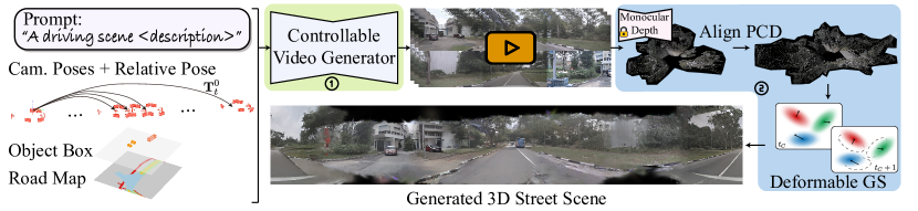
Figure 2: Method Overview of MagicDrive3D. For controllable street scene generation, MagicDrive3D decomposes the task into two steps: ① conditional multi-view video generation, which tackles the control signals and provides detailed prior of the scene; and ② scene reconstruction with deformable Gaussian splatting, which guarantees view consistency for any-view rendering.

4.1 3D Street Scene Generation

Direct modeling of controllable street scene generation faces two major challenges: scene dynamics and discrepancy in data collection. Scene dynamics refer to the movements and deformation of elements in the scene, while discrepancy in data collection refer to the discrepancy (e.g., exposure) caused by data collection. These two challenges are even more severe due to the sparsity of cameras for street views (e.g., typically only 6 surrounding perspective cameras). Therefore, reconstruction-generation frameworks do not work well for street scene generation [13, 2].

Figure 2 shows the overview of MagicDrive3D. Given scene descriptions $\mathbf{S}$ as input, MagicDrive3D first extend the descriptions into sequence $\{\mathbf{S}_{t}\}$, where $t\in[0,T]$ according to preset camera poses $\{\mathbf{P}_{c,t}\}$, and generate a sequence of successive multi-view images $\{\mathcal{I}_{c,t}\}$, where $c\in\{1,\dots,N\}$ refers to $N$ surrounding cameras, according to conditions $\{\mathbf{S}_{t},\mathbf{P}_{c,t}\}$ (detailed in Section 4.2). Then we construct Gaussian representation of the scene with $\{\mathcal{I}_{c,t}\}$ and camera poses $\{\mathbf{P}_{c,t}\}$ as input. This step contains an initializing procedure with a pre-trained monocular depth model and an optimizing process with deformable Gaussian splatting (detailed in Section 4.3). Consequently, the generated street scene not only supports any-view rendering, but also accurately reflects different control signals.

MagicDrive3D integrate geometry-free view synthesis and geometry-focused reconstruction, where control signals are tackled by a multi-view video generator, while reconstruction step guarantee the generalization ability for any-view rendering. Such a video generator has two advantages: first, since multi-view video generation does not require generalization on novel views [9], it poses less data dependency for street scenes; second, through conditional training, the model is capable of decomposition of control signals, and thus turns dynamic scenes into static scenes which are more friendly for reconstruction. Besides, for the reconstruction step, strong prior from the multi-view video reduces the burden for scene modeling with complex details.

4.2 Relative Pose Control for Video Generation

Given scene descriptions and a sequence of camera poses $\{\mathbf{S}_{t},\mathbf{P}_{c,t}\}$, our video generator is responsible for multi-view video generation. Although many previous art for street view generation achieve expressive visual effects, such as [9, 32, 30, 29], their formulations leave out a crucial requirement for 3D modeling. Specifically, the camera pose $\mathbf{P}_{c,t}$ is typically relative to the LiDAR coordinate of each frame. Thus, there is no precise control signal related to the ego trajectory, which significantly determine the geometric relationship between views of different $t$s.

In our video generation model, we amend such precise control ability by adding the transformation between each frame to the first frame, i.e., $\mathbf{T}^{0}_{t}$. To properly encode such information, we adopt Fourier embedding with Multi-Layer Perception (MLP), and concatenate the embedding with the original embedding of $\mathbf{P}_{c,t}$, similar to [9]. As a result, our video generator provides better 3D consistency across frames, most importantly, making the camera poses to each view available in the same coordinate, i.e., $[\mathbf{R}^{0}_{c,t},\mathbf{t}^{0}_{c,t}]=\mathbf{T}^{0}_{t}[\mathbf{R}_{c,t},\mathbf{t}_{c,t}]$.

4.3 Enhanced Gaussian Splatting for Generated Content

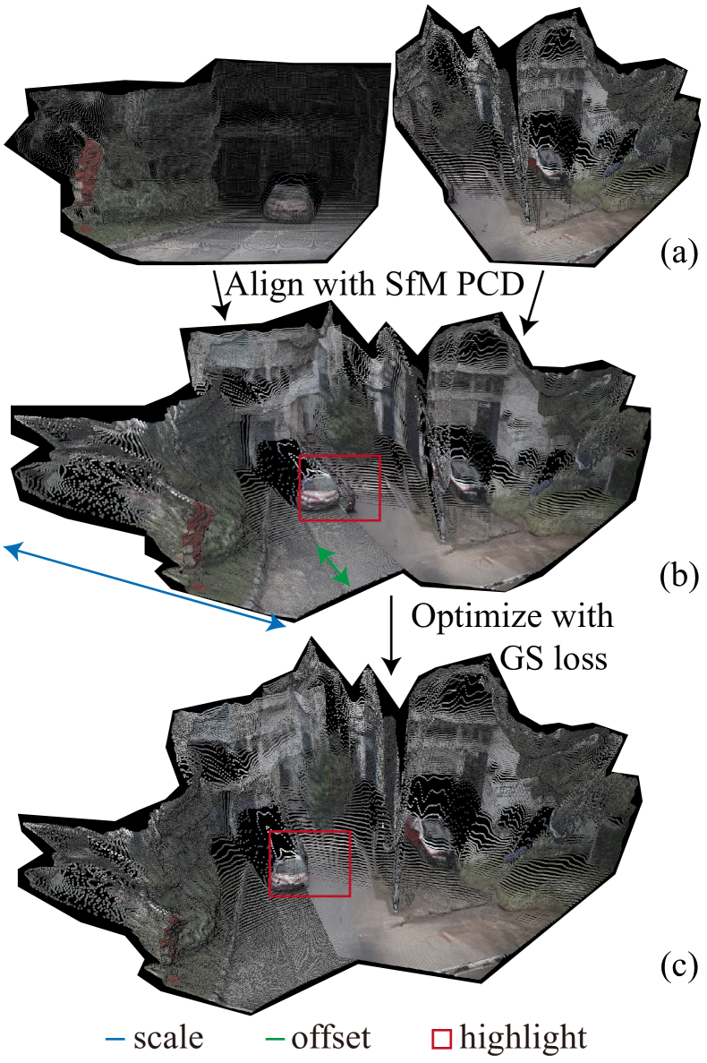
Figure 3: We optimize the monocular depths (a) with 2 steps for better alignment: coarse scale/offset estimation with SfM PCD (b) and GS optimization (c).

As introduced in Section 3, 3DGS is a flexible explicit representation for scene reconstruction. Besides, the fast training and rendering speed of 3DGS make it highly suitable for reducing generation costs in our scene creation pipeline. However, similar to other 3D reconstruction methods, 3DGS necessitates a high level of cross-view 3D consistency at the pixel level, which unavoidably magnifies the minute errors in the generated data into conspicuous artifacts. Therefore, we propose improvements for 3DGS from the perspectives of prior, modeling, and loss, enabling 3DGS to tolerate minor errors in the generated camera view, thereby becoming a potent tool for enhancing geometric consistency in rendering.

Prior: Consistent Depth Prior. As essential geometry information, depth is extensively utilized in street scene reconstruction, such as the depth value from LiDAR or other depth sensors used in [33, 34]. However, for synthesized camera views, the depth is unavailable. Therefore, we propose to use pre-trained monocular depth estimator [3] to infer depth information.

While monocular depth estimation is separate for each camera view, proper scale $s_{c,t}$ and offset $b_{c,t}$ parameters should be estimated to align them for a single scene [38], as in Figure 3(a). To this end, we first apply the Point Cloud (PCD) from Structure of Motion (SfM) [24, 23], shown in Figure 3(b). However, such PCD is too sparse to accurately restore $(s_{c,t},b_{c,t})$ for any views. To bridge the final gap, secondly, we propose further optimizing the $(s_{c,t},b_{c,t})$ using the GS loss, as in Figure 3(c). Specifically, we replace the optimization for Guassian centers $\boldsymbol{\mu}_{i}$ with $(s_{c,t},b_{c,t})$. After the optimization, we initialize $\boldsymbol{\mu}_{i}$ with points from depth values. Since GS algorithm is sensitive to accurate point initialization [12, 8], our method provides useful prior to reconstructing in this sparse view scenario.

Modeling: Deformable Gaussians for Local Dynamic. Despite the 3D geometric consistency provided by our video generation model, there are inevitably pixel-level disparities in some object details, as shown in Figure 4. The strict consistency assumption of 3DGS may amplify these minor errors, resulting in floater artifacts. To mitigate the impact of these errors, we propose Deformable Gaussian Splitting (DGS), which, based on 3DGS, reduces the requirement for temporal consistency between frames, thereby ensuring the reconstruction effect of the generated viewpoint.

Specifically, as shown in Figure 4, we pick the center frame $t=t_{C}$ as the canonical space and enforce all Gaussians in this space. Hence, we allocate a set of offsets to each Gaussian, $\boldsymbol{\mu}^{o}_{p}(t)\in\mathbb{R}^{3}$, where $t\in[1,\dots,T]$ and $\boldsymbol{\mu}^{o}_{p}(t_{C})\equiv\mathbf{0}$. Note that, different camera views from the same $t$ share the same $\boldsymbol{\mu}^{o}_{p}(t)$ for each Gaussian, and we apply regularization on them to keep the dynamic in local, as shown in Equation 2:

$$\mathcal{L}_{\text{reg}_{o}}=\|\boldsymbol{\mu}^{o}(t)\|_{2}.$$ (2)

Consequently, $\boldsymbol{\mu}^{o}_{p}(t)$ can manage the local dynamics driven by pixel-level disparities, while $\boldsymbol{\mu}$ focuses on the global geometric correlations. It ensures the quality of scene reconstruction by leveraging consistent parts across different viewpoints, simultaneously eliminating artifacts. Besides, with the analytical gradient w.r.t. $SE(3)$ pose of cameras [17], we also make the camera pose optimizable in the final few steps of GS iterations, which helps to mitigate the local dynamic from camera poses.

Figure 4: Illustration of the local dynamic from two successive generated frames of Front-Left (FL) camera. Even though our video generation model retains fine 3D consistency, minor discrepancies are inevitable. Our DGS can effectively reconstruct the scene with awareness of such discrepancy.

Loss: Aligning Exposure with Appearance Modeling. Typical street view dataset is collected with multiple cameras, which capture views independently through auto-exposure and auto-white-balance [4]. Since the video generation is optimized to match the original data distribution, the differences from different cameras also exist in the generated data. The appearance differences are well-known issues for in-the-wild reconstruction [16]. In this paper, we propose a dedicated appearance modeling technique for GS representation.

We hypothesize that the disparity between different views can be represented by affine transformations $\mathbf{A}_{i}(\cdot)$ for $i$-th camera view. An Appearance Embedding (AE) map $\mathbf{e}_{i}\in\mathbb{R}^{w_{e}\times h_{e}\times c_{e}}$ is allocated for each view, and a Convolutional Neural Network (CNN) is utilized to approximate this transformation matrix $w_{\mathbf{A}}\in\mathbb{R}^{w\times h\times 3}$. The final computation of the pixel-wise $\ell_{1}$ loss is conducted using the transformed image. Therefore, our final loss for DGS is as follows:

$$\mathcal{L}_{\text{DGS}}=\mathcal{L}_{\text{AEGS}}+\lambda_{{\text{reg}_{o}}}\mathcal{L}_{{\text{reg}_{o}}}=(1-\lambda)\mathcal{L}_{1}(\mathbf{A}_{i}(\mathcal{I}^{r}_{i}),\mathcal{I}_{i})+\lambda\mathcal{L}_{\text{D-SSIM}}(\mathcal{I}^{r}_{i},\mathcal{I}_{i})+\lambda_{{\text{reg}_{o}}}\mathcal{L}_{{\text{reg}_{o}}},$$ (3)

where $\lambda_{{\text{reg}_{o}}}$ is the hyper-parameter for offset regularization.

Algorithm 1 Enhanced Deformable GS

1:camera views $\{\mathcal{I}_{i}\}$, camera parameters $\{\mathbf{P}^{0}_{i}\}$, monocular depth $\{\mathcal{D}_{i}\}$, optimization steps for depth $s_{D}$, camera pose $s_{\text{C}}$, and GS $s_{\text{GS}}$

2:DGS of the scene $\{\boldsymbol{\mu}_{p},\boldsymbol{\mu}^{o}_{p},\boldsymbol{\Sigma}_{p},\text{SH}_{p}\}$, and optimized camera pose $\{\mathbf{P}^{0}_{i}\}$

3:$\mathcal{P}_{SfM}=$ PCD from SfM

4:Optimize $(s_{c,t},b_{c,t})$ with $\mathcal{P}_{\text{SfM}}$ for each $\{c,t\}$

5:Random initialize AEs $\{\mathbf{e}_{i}\}$

6:for step in $1,\dots,s_{D}$ do

7:    Random pick one view $\mathcal{I}_{i}$

8:    $\mathcal{L}=\mathcal{L}_{\text{AEGS}}(\mathcal{I}_{i},\mathcal{I}^{r}_{i},\mathbf{e}_{i})$

9:    Update $(s,b),\mathbf{e}_{i},\boldsymbol{\Sigma},\text{SH}$ with $\nabla\mathcal{L}$

10:end for

11:Initialize $\boldsymbol{\mu}$ with $(s,b)$ and $\mathcal{D}$

12:for step in $s_{D},\dots,s_{\text{GS}}$ do

13:    Random pick one view $\mathcal{I}_{i}$ and get its $t$

14:    $\mathcal{L}=\mathcal{L}_{\text{DGS}}(\mathcal{I}_{i},\mathcal{I}^{r}_{i},\mathbf{e}_{i},\boldsymbol{\mu}^{o}(t))$

15:    Update $\boldsymbol{\mu},\boldsymbol{\mu}^{o}(t),\mathbf{e}_{i},\boldsymbol{\Sigma},\text{SH}$ with $\nabla\mathcal{L}$

16:    if step $>s_{\text{C}}$ then

17:         Update $\mathbf{P}^{0}_{i}$ with $\nabla\mathcal{L}$

18:    end if

19:end for

Optimization Flow. We demonstrate the overall optimization flow of the proposed DGS in Algorithm 1. Line 2 is the first optimization of monocular depths. Lines 4-8 refer to the second optimization of the monocular depths. Lines 10-16 are the main loop for DGS reconstruction, where we consider temporal offsets on Gaussians, camera pose optimization for local dynamics, and AEs for appearance discrepancies among views.

5 Experiments

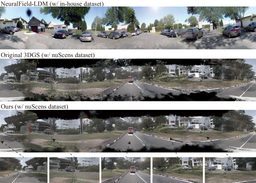
Figure 5: Qualitative comparison with NF-LDM (figure from [13]) and original 3DGS (on the same generated video). Panoramas for GS are transformed and stitched from perspective cameras with $90^{\circ}$ FOV. Views in the last row are rendered with camera rigs different from the nuScenes dataset.

5.1 Experimental Setup

Dataset. We test our MagicDrive3D using the nuScenes dataset [4], which is commonly used for generating and reconstructing street views [9, 32, 30, 33]. The official configuration is followed, using 700 street-view video clips of approximately 20s each for training and another 150 clips for validation. For semantics in control signals, we follow [9], using 10 object classes and 8 road classes.

Table 1: Two settings for reconstruction quality evaluation. Testing views are in green while training views are in red.

name	#test	#train	camera poses
360∘	6	90
vary-t	12	84

Metrics and Settings. MagicDrive3D is primarily evaluated using the Fréchet Inception Distance (FID) by rendering novel views unseen in the dataset and comparing their FID with real images. In addition, the method’s video generation ability is evaluated using Fréchet Video Distance (FVD), and its reconstruction performance is assessed using L1, PSNR, SSIM [31], and LPIPS [35]. For reconstruction evaluation, two testing scenarios are employed: 360^∘, where all six views from $t=9$ are reserved for testing the reconstruction in the canonical space; and vary-t, where one view is randomly sampled from different $t$ to assess long-range reconstruction ability through $t$ in the canonical space (as shown in Table 1).

Implementation. For video generation, we train our generator based on the pre-trained street view image generation model from [9]. By adding the proposed relative pose control, we train 4 epochs (77040 steps) on the nuScenes training set with a learning rate of $8e^{-5}$. We follow the settings for 7-frame videos described in [9], using $224\times 400$ for each view but extending to $T=16$ frames. Consequently, for reconstruction, we select $t=8$ as the canonical space. Except we change the first 500 steps to optimize $(s_{c,t},b_{c,t})$ for each view and $\lambda_{\text{reg}_{o}}=1.0$, other settings are the same as 3DGS.

5.2 Main Results

Table 2: Generation quality evaluation. All validation scenes from the nuScenes dataset are adopted. We use all generated views for reconstruction. Novel views adopt camera poses different from the nuScenes.

Methods	FVD	FID (seen)	FID (novel)
MD [9] ($T=16$)	177.26	20.92	N/A
Ours (video gen.)	164.72	20.67	N/A
3DGS	N/A	45.07	145.72
Ours (scene gen.)	N/A	23.99	34.45

Generation Quality. As shown in Table 2, the evaluation of generation quality involves two aspects. Firstly, the quality of video generation is assessed using extended 16-frame MagicDrive [9] as a baseline. Despite minor improvement in single-frame quality based on FID, MagicDrive3D substantially enhances video quality (as evidenced by FVD), demonstrating the efficacy of the proposed relative camera pose embedding in enhancing temporal consistency. Secondly, the image quality of renderings from the generated scene is evaluated using FID. We also include qualitative comparisons in Figure 5. Compared to 3DGS, our enhanced DGS significantly enhances visual quality in reconstructing contents, particularly in unseen novel views.

Reconstruction Quality. Our enhanced DGS, as a reconstruction method, is further evaluated by comparing renderings with ground truth (GT) images. Here, the generated views from the video generator are treated as GT. We employ two settings per Table 1, with results displayed in Table 3. As per all metrics, our enhanced DGS not only improves reconstruction quality for training views but also drastically enhances quality for testing views, compared to 3DGS.

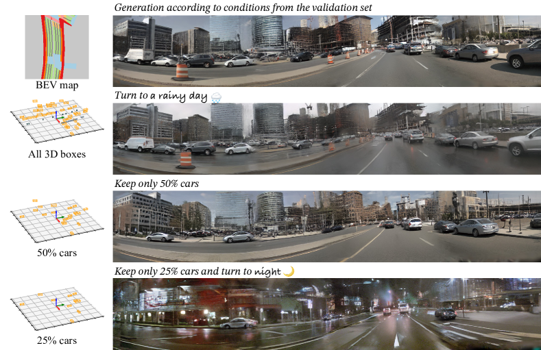
Figure 6: Qualitative evaluation for controllability (we show the view from back-left to front-right area). By changing different control signals, MagicDrive3D can edit the scene from different levels.

Table 3: Reconstruction quality evaluation. We random sample 100 scenes from the nuScenes validation set for evaluation. “cc” refers to color correction from [1]. Although 3DGS does not consider appearance differences, we apply “cc” to it for fair comparisons.

Settings		Methods	L1 $\downarrow$	PSNR $\uparrow$	SSIM $\uparrow$	LPIPS $\downarrow$
train view	vary-t	3DGS	0.0189	30.1191	0.9261	0.1259
		3DGS + cc	0.0186	30.2498	0.9253	0.1258
		Ours	0.0167	32.6001	0.9544	0.0673
	360∘	3DGS	0.0202	29.4943	0.9187	0.1365
		3DGS + cc	0.0199	29.6327	0.9178	0.1366
		Ours	0.0174	32.2104	0.9530	0.0693
test view	vary-t	3DGS	0.0890	17.9879	0.4378	0.4648
		3DGS + cc	0.0799	19.1387	0.4814	0.4697
		Ours	0.0738	19.7063	0.5145	0.4115
	360∘	3DGS	0.0910	17.8322	0.4318	0.4756
		3DGS + cc	0.0804	19.0773	0.4777	0.4796
		Ours	0.0622	21.0351	0.5754	0.3207

Controllability. MagicDrive3D accepts 3D bounding boxes, BEV map, and text as control signals, each of which possesses the capacity to independently manipulate the scene. To show such controllability, we edit a scene from the nuScenes validation set, as presented in Figure 6. Clearly, MagicDrive3D can effectively alter the generation of the scene to align with various control signals while maintaining 3D geometric consistency.

5.3 Ablation Study

Ablation on Enhanced Gaussian Splatting. As detailed in Section 4.3, three enhancements - prior, modeling, and loss - have been made to 3DGS. To evaluate their efficacy, each was ablated from the final algorithm, the results of which are shown in Table 4. Notations “w/o depth scale opt” and “w/o depth opt” represent the absence of GS loss optimization for $(s_{c,t},b_{c,t})$ and use of direct output from the monocular depth model, respectively. Each component’s removal lowered the method’s performance, while incorrect depth sometimes performs worse than the 3DGS baseline. Removal of AE in “vary-t” led to inferior PSNR but improved LPIPS, which is reasonable because AE mitigates the pixel-wise color constraint during reconstruction.

Table 4: Ablation study on enhanced DGS. We adopt the same settings as in Table 3, where 100 scenes from the nuScenes validation set are adopted.

setting	method	L1 $\downarrow$	PSNR $\uparrow$	SSIM $\uparrow$	LPIPS $\downarrow$
vary-t	3DGS	0.0799	19.1387	0.4814	0.4697
	w/o AE	0.0822	18.8467	0.4758	0.4452
	w/o depth scale opt	0.0815	18.8885	0.4767	0.4366
	w/o depth opt.	0.1046	17.2776	0.4399	0.5545
	w/o xyz offset + cam	0.0798	19.1657	0.4919	0.4580
	Ours	0.0738	19.7063	0.5145	0.4115
360∘	3DGS	0.0804	19.0773	0.4777	0.4796
	w/o AE	0.0722	19.7742	0.5114	0.3791
	w/o depth scale opt	0.0736	19.6501	0.5086	0.3736
	w/o depth opt	0.0995	17.6707	0.4487	0.5150
	w/o xyz offset + cam	0.0798	19.1682	0.4888	0.4663
	Ours	0.0622	21.0351	0.5754	0.3207

5.4 Application

Training Support for Perception Tasks. We demonstrate an application wherein street scene generation serves as a data engine for perception tasks, leveraging the advantage of any-view rendering to improve viewpoint robustness [14]. We employ CVT [37] and the BEV segmentation task following the evaluation protocols of [37, 9]. By incorporating 4 different rigs on the FRONT camera and adding rendered views for training, the negative impact from viewpoint changes is alleviated (Table 5), exemplifying the utility of street scene generation in training perception tasks.

Table 5: MagicDrive3D improves the viewpoint robustness [14] of CVT [37]. All results are mIoU for BEV segmentation. Colors highlight the differences with baseline. The best results are in bold.

Setting	Method		no rig	depth+0.5m	pitch-5∘	yaw+5∘	yaw-5∘
vehicle	only real data		17.14	16.63	15.50	16.99	15.94
	w/ render view (no rig)		20.67 +3.53	20.13 +3.50	17.03 +1.53	19.40 +2.41	19.30 +3.36
	w/ random aug. of 4 rigs		21.05 +3.91	20.46 +3.83	19.75 +4.25	19.81 +2.82	19.83 +3.89
road	only real data		54.94	54.56	53.82	54.20	53.67
	w/ render view (no rig)		60.31 +5.37	59.93 +5.37	58.46 +4.64	59.16 +4.96	59.32 +5.65
	w/ random aug. of 4 rigs		60.59 +5.65	60.38 +5.82	59.95 +6.13	60.21 +6.01	60.29 +6.62

6 Conclusion and Discussion

This paper introduces MagicDrive3D, a unique 3D street scene generation framework that integrates geometry-free view synthesis and geometry-focused 3D representations. MagicDrive3D significantly reduces data requirements, enabling training on typical autonomous driving datasets, such as nuScenes. Within the generation-reconstruction pipeline, MagicDrive3D employs a video generation model to enhance inter-frame consistency, while the enhanced deformable GS improves reconstruction quality from generated views. Comprehensive experiments demonstrate that MagicDrive3D can produce high-quality 3D street scenes with multi-level controls. Additionally, we show that scene generation can serve as a data engine for perception tasks such as BEV segmentation.

Limitation and Future Work. As a data-centric method, MagicDrive3D sometimes struggles to generate complex objects like pedestrians, whose appearances are intricate. Additionally, areas with high texture detail (e.g., road fences) or small spatial features (e.g., light poles) are occasionally poorly generated due to limitations in the reconstruction method. Future work may focus on addressing these challenges and further improving the quality and robustness of generated 3D scenes.

APPENDIX

Appendix A More Implementation Details

For the monocular depth model, we use ZoeDepth [3]. Although it is trained for metric depth estimation, due to domain differences, raw estimation is not usable, as shown in Section 5.3 and Figure 3. Methodologically, MagicDrive3D does not rely on a specific depth estimation model. Better estimations can further improve our scene generation quality.

Since GS only supports perspective rendering, to stitch the view for panorama, we use code from perspective to equirectangular transformation provided by https://github.com/timy90022/Perspective-and-Equirectangular.

All our experiments are conducted with NVIDIA V100 32GB GPUs. The generation of a single scene takes about 2 minutes for video generation and about 30 minutes for deformable GS reconstruction. For reference, 3DGS reconstruction typically takes about 23 minutes for scenes of similar scales. Therefore, the proposed enhancement is efficient. As for rendering, there is no additional computation for our method compared with 3DGS.

Appendix B Comparison with Simple Baseline

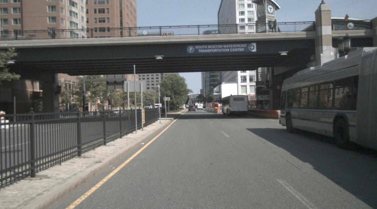
(a) Conditional image to LucidDreamer [6]

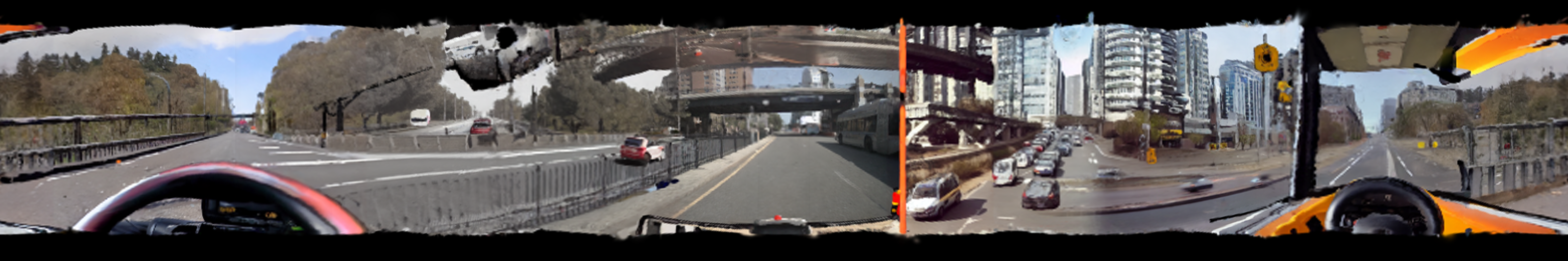
(b) Scene generated by LucidDreamer [6], with text “A driving scene in the city from the front camera of the vehicle. A bus on the right side. There is a bridge overhead. There is a railing in the center of the left road. Some vehicles ahead”

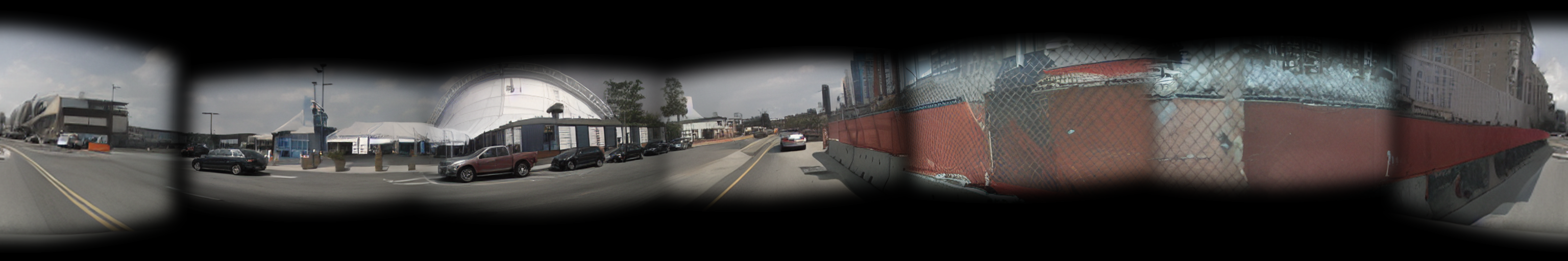
(c) Stitched panorama with real camera views from nuScenes dataset. Due to the limited overlaps, there are many empty (black) areas.

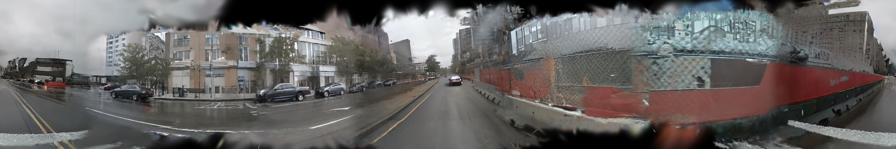
(d) Panorama from MagicDrive3D. The scene is generated with the same object boxes and BEV map as Figure 7(c), but turned to “rainy day”.

Figure 7: Comparison with two baselines: LucidDreamer [6] and direct stitching real images.

As shown in Figure 7, we further compare MagicDrive3D with two baselines, i.e., LucidDreamer [6] and directly stitching real data. The former method has been proposed recently and takes text description as the only condition. Thus, it is hard to generate photo-realistic street scenes. When providing multi-view video frames from nuScenes with known camera poses, their pipeline fails to reconstruct. We suppose the reason is limited overlaps and errors from depth estimation. As suggested by the released code, we changed the image generation model to lllyasviel/control_v11p_sd15_inpaint for inpainting by providing a nuScenes image, i.e., Figure 7(a). However, due to the lack of controllability, the results from LucidDream (e.g., Figure 7(b)) are unsatisfactory. As for the latter one, as shown in Figure 7(c), it is also bad due to the limited overlaps between views. On the contrary, the scene generated from MagicDrive3D can render continuous panorama, as shown in Figure 7(d), which is also controllable through multiple conditions.

Note that, panorama generation is only one of the applications of our generated scenes. We show them just for convenient qualitative comparison within the paper. Since our scene generation contains geometric information, they can be rendered from any camera view, as shown in Figure 5.

Appendix C Implementation Detail of Appearance Embedding

We show in Figure 8 the detailed architecture of the CNN used in our appearance modeling. The AE map is $32\times$ smaller than the input image to reduce the computational cost. Hence, we first downsample the input image by $32\times$. Then, we use $3\times 3$ convolution for feature extraction and pixel shuffle for upsampling. Each convolution layer is activated by ReLU.

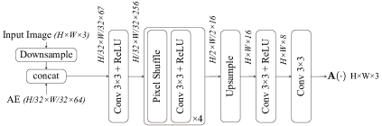
Figure 8: The CNN architecture of appearance modeling, as introduced in Section 4.3.

Appendix D Broader Impacts

The implementation of MagicDrive3D in controllable 3D street scene generation could potentially revolutionize the autonomous driving industry. By creating detailed 3D scenarios, self-driving vehicles can be trained more effectively and efficiently for real-world applications, thereby leading to improved safety and accuracy. Moreover, it could potentially provide realistic simulations for human-operated vehicle testing and training, thus contributing to reducing the occurrence of accidents on the roads while enhancing driver expertise. In the broader scope, MagicDrive3D could be of considerable value to the virtual reality industry and video gaming industry, enabling these sectors to generate more lifelike 3D scenes and intricate gaming experiences.

On the downside, the development and application of such advanced technology could lead to certain unwanted scenarios. For instance, the increased automation in industries, driven by the potential of this technology, could lead to job losses for drivers and other related professionals as their roles become automated. A societal transition will be needed to avoid negative impacts on employment levels and the fairness of wealth distribution.

Appendix E More Qualitative Results

We show more generated street scenes from MagicDrive3D in Figure 9.

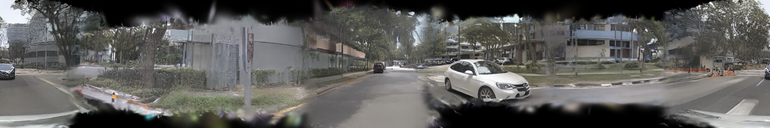
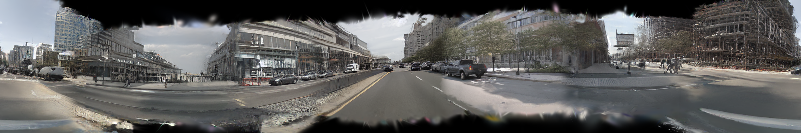
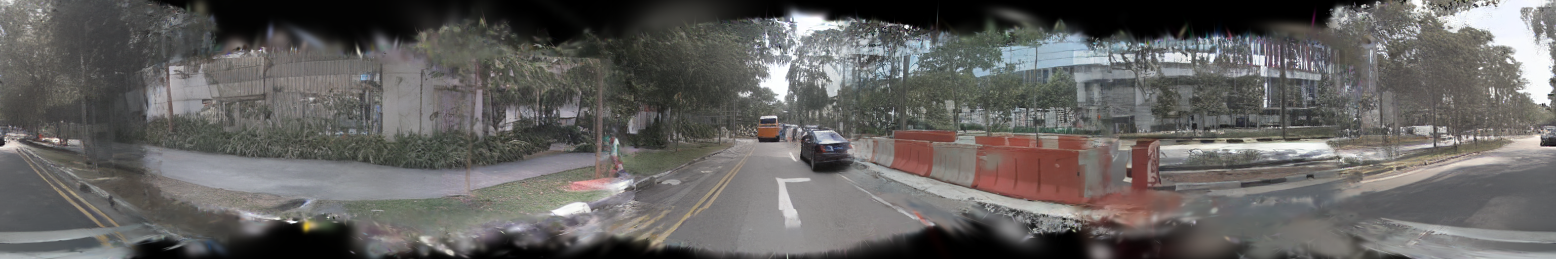
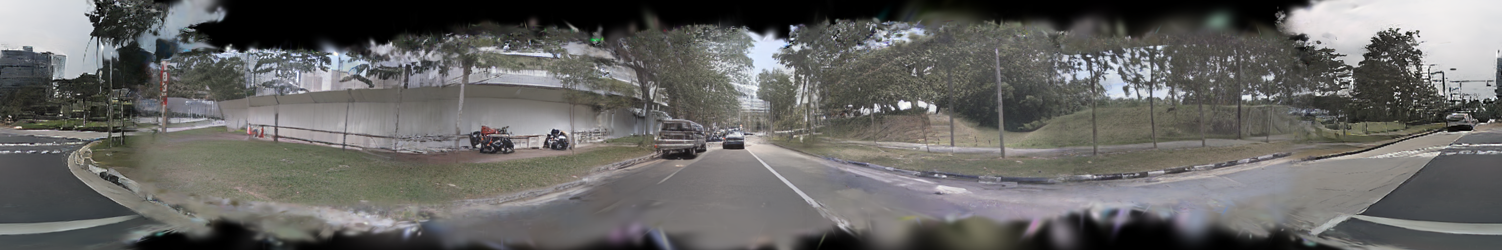
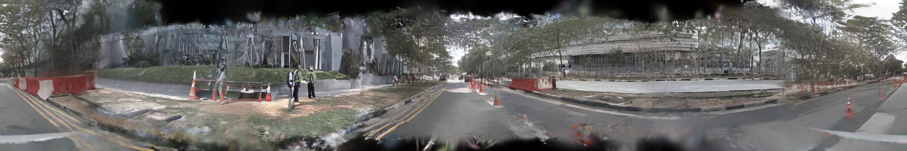
Figure 9: Generated street scenes from MagicDrive3D. We adopt control signals from nuScenes validation set.

References

- [1] Jonathan T. Barron, Ben Mildenhall, Dor Verbin, Pratul P. Srinivasan, and Peter Hedman. Mip-nerf 360: Unbounded anti-aliased neural radiance fields. In CVPR, 2022.
- [2] Miguel Angel Bautista, Pengsheng Guo, Samira Abnar, Walter Talbott, Alexander Toshev, Zhuoyuan Chen, Laurent Dinh, Shuangfei Zhai, Hanlin Goh, Daniel Ulbricht, et al. Gaudi: A neural architect for immersive 3d scene generation. In NeurIPS, 2022.
- [3] Shariq Farooq Bhat, Reiner Birkl, Diana Wofk, Peter Wonka, and Matthias Müller. Zoedepth: Zero-shot transfer by combining relative and metric depth. arXiv preprint arXiv:2302.12288, 2023.
- [4] Holger Caesar, Varun Bankiti, Alex H Lang, Sourabh Vora, Venice Erin Liong, Qiang Xu, Anush Krishnan, Yu Pan, Giancarlo Baldan, and Oscar Beijbom. nuscenes: A multimodal dataset for autonomous driving. In CVPR, 2020.
- [5] Kai Chen, Enze Xie, Zhe Chen, Yibo Wang, Lanqing HONG, Zhenguo Li, and Dit-Yan Yeung. Geodiffusion: Text-prompted geometric control for object detection data generation. In ICLR, 2024.
- [6] Jaeyoung Chung, Suyoung Lee, Hyeongjin Nam, Jaerin Lee, and Kyoung Mu Lee. Luciddreamer: Domain-free generation of 3d gaussian splatting scenes. arXiv preprint arXiv:2311.13384, 2023.
- [7] Terrance DeVries, Miguel Angel Bautista, Nitish Srivastava, Graham W Taylor, and Joshua M Susskind. Unconstrained scene generation with locally conditioned radiance fields. In ICCV, 2021.
- [8] Zhiwen Fan, Wenyan Cong, Kairun Wen, Kevin Wang, Jian Zhang, Xinghao Ding, Danfei Xu, Boris Ivanovic, Marco Pavone, Georgios Pavlakos, Zhangyang Wang, and Yue Wang. Instantsplat: Unbounded sparse-view pose-free gaussian splatting in 40 seconds. arXiv preprint arXiv:2403.20309, 2024.
- [9] Ruiyuan Gao, Kai Chen, Enze Xie, Lanqing Hong, Zhenguo Li, Dit-Yan Yeung, and Qiang Xu. MagicDrive: Street view generation with diverse 3d geometry control. In ICLR, 2024.
- [10] Ian Goodfellow, Jean Pouget-Abadie, Mehdi Mirza, Bing Xu, David Warde-Farley, Sherjil Ozair, Aaron Courville, and Yoshua Bengio. Generative adversarial nets. In NeurIPS, 2014.
- [11] Jonathan Ho, Ajay Jain, and Pieter Abbeel. Denoising diffusion probabilistic models. In NeurIPS, 2020.
- [12] Bernhard Kerbl, Georgios Kopanas, Thomas Leimkühler, and George Drettakis. 3d gaussian splatting for real-time radiance field rendering. ACM Transactions on Graphics, 42(4), July 2023.
- [13] Seung Wook Kim, Bradley Brown, Kangxue Yin, Karsten Kreis, Katja Schwarz, Daiqing Li, Robin Rombach, Antonio Torralba, and Sanja Fidler. Neuralfield-ldm: Scene generation with hierarchical latent diffusion models. In CVPR, 2023.
- [14] Tzofi Klinghoffer, Jonah Philion, Wenzheng Chen, Or Litany, Zan Gojcic, Jungseock Joo, Ramesh Raskar, Sanja Fidler, and Jose M Alvarez. Towards viewpoint robustness in bird’s eye view segmentation. In ICCV, 2023.
- [15] Jiaqi Lin, Zhihao Li, Xiao Tang, Jianzhuang Liu, Shiyong Liu, Jiayue Liu, Yangdi Lu, Xiaofei Wu, Songcen Xu, Youliang Yan, and Wenming Yang. Vastgaussian: Vast 3d gaussians for large scene reconstruction. In CVPR, 2024.
- [16] Ricardo Martin-Brualla, Noha Radwan, Mehdi S. M. Sajjadi, Jonathan T. Barron, Alexey Dosovitskiy, and Daniel Duckworth. NeRF in the Wild: Neural Radiance Fields for Unconstrained Photo Collections. In CVPR, 2021.
- [17] Hidenobu Matsuki, Riku Murai, Paul H. J. Kelly, and Andrew J. Davison. Gaussian Splatting SLAM. In CVPR, 2024.
- [18] Ben Mildenhall, Pratul P Srinivasan, Matthew Tancik, Jonathan T Barron, Ravi Ramamoorthi, and Ren Ng. Nerf: Representing scenes as neural radiance fields for view synthesis. In ECCV, 2020.
- [19] Ben Poole, Ajay Jain, Jonathan T Barron, and Ben Mildenhall. Dreamfusion: Text-to-3d using 2d diffusion. In ICLR, 2022.
- [20] Konstantinos Rematas, Andrew Liu, Pratul P. Srinivasan, Jonathan T. Barron, Andrea Tagliasacchi, Tom Funkhouser, and Vittorio Ferrari. Urban radiance fields. In CVPR, 2022.
- [21] Robin Rombach, Andreas Blattmann, Dominik Lorenz, Patrick Esser, and Björn Ommer. High-resolution image synthesis with latent diffusion models. In CVPR, 2022.
- [22] Robin Rombach, Patrick Esser, and Björn Ommer. Geometry-free view synthesis: Transformers and no 3d priors. In ICCV, 2021.
- [23] Johannes Lutz Schönberger and Jan-Michael Frahm. Structure-from-motion revisited. In CVPR, 2016.
- [24] Johannes Lutz Schönberger, Enliang Zheng, Marc Pollefeys, and Jan-Michael Frahm. Pixelwise view selection for unstructured multi-view stereo. In ECCV, 2016.
- [25] Yang Song, Jascha Sohl-Dickstein, Diederik P Kingma, Abhishek Kumar, Stefano Ermon, and Ben Poole. Score-based generative modeling through stochastic differential equations. In ICLR, 2020.
- [26] Jiaxiang Tang, Jiawei Ren, Hang Zhou, Ziwei Liu, and Gang Zeng. Dreamgaussian: Generative gaussian splatting for efficient 3d content creation. arXiv preprint arXiv:2309.16653, 2023.
- [27] Jiaxiang Tang, Jiawei Ren, Hang Zhou, Ziwei Liu, and Gang Zeng. Dreamgaussian: Generative gaussian splatting for efficient 3d content creation. In ICLR, 2024.
- [28] Arash Vahdat, Francis Williams, Zan Gojcic, Or Litany, Sanja Fidler, Karsten Kreis, et al. Lion: Latent point diffusion models for 3d shape generation. In NeurIPS, 2022.
- [29] Xiaofeng Wang, Zheng Zhu, Guan Huang, Xinze Chen, Jiagang Zhu, and Jiwen Lu. Drivedreamer: Towards real-world-driven world models for autonomous driving. arXiv preprint arXiv:2309.09777, 2023.
- [30] Yuqi Wang, Jiawei He, Lue Fan, Hongxin Li, Yuntao Chen, and Zhaoxiang Zhang. Driving into the future: Multiview visual forecasting and planning with world model for autonomous driving. arXiv preprint arXiv:2311.17918, 2023.
- [31] Zhou Wang, Alan C Bovik, Hamid R Sheikh, and Eero P Simoncelli. Image quality assessment: from error visibility to structural similarity. IEEE transactions on image processing, 13(4):600–612, 2004.
- [32] Yuqing Wen, Yucheng Zhao, Yingfei Liu, Fan Jia, Yanhui Wang, Chong Luo, Chi Zhang, Tiancai Wang, Xiaoyan Sun, and Xiangyu Zhang. Panacea: Panoramic and controllable video generation for autonomous driving. arXiv preprint arXiv:2311.16813, 2023.
- [33] Ziyang Xie, Junge Zhang, Wenye Li, Feihu Zhang, and Li Zhang. S-nerf: Neural radiance fields for street views. In ICLR 2023, 2023.
- [34] Yunzhi Yan, Haotong Lin, Chenxu Zhou, Weijie Wang, Haiyang Sun, Kun Zhan, Xianpeng Lang, Xiaowei Zhou, and Sida Peng. Street gaussians for modeling dynamic urban scenes. arXiv preprint arXiv:2401.01339, 2024.
- [35] Richard Zhang, Phillip Isola, Alexei A Efros, Eli Shechtman, and Oliver Wang. The unreasonable effectiveness of deep features as a perceptual metric. In CVPR, 2018.
- [36] Xiaoming Zhao, R Alex Colburn, Fangchang Ma, Miguel Ángel Bautista, Joshua M. Susskind, and Alex Schwing. Pseudo-generalized dynamic view synthesis from a video. In ICLR, 2024.
- [37] Brady Zhou and Philipp Krähenbühl. Cross-view transformers for real-time map-view semantic segmentation. In CVPR, 2022.
- [38] Kaichen Zhou, Jia-Xing Zhong, Sangyun Shin, Kai Lu, Yiyuan Yang, Andrew Markham, and Niki Trigoni. Dynpoint: Dynamic neural point for view synthesis. In NeurIPS, 2024.
- [39] Matthias Zwicker, Hanspeter Pfister, Jeroen Van Baar, and Markus Gross. Ewa volume splatting. In Proceedings Visualization, 2001. VIS’01., 2001.