Time Cell Inspired Temporal Codebook in Spiking Neural Networks for Enhanced Image Generation

Abstract

This paper presents a novel approach leveraging Spiking Neural Networks (SNNs) to construct a Variational Quantized Autoencoder (VQ-VAE) with a temporal codebook inspired by hippocampal time cells. This design captures and utilizes temporal dependencies, significantly enhancing the generative capabilities of SNNs. Neuroscientific research has identified hippocampal "time cells" that fire sequentially during temporally structured experiences. Our temporal codebook emulates this behavior by triggering the activation of time cell populations based on similarity measures as input stimuli pass through it. We conducted extensive experiments on standard benchmark datasets, including MNIST, FashionMNIST, CIFAR10, CelebA, and downsampled LSUN Bedroom, to validate our model’s performance. Furthermore, we evaluated the effectiveness of the temporal codebook on neuromorphic datasets NMNIST and DVS-CIFAR10, and demonstrated the model’s capability with high-resolution datasets such as CelebA-HQ, LSUN Bedroom, and LSUN Church. The experimental results indicate that our method consistently outperforms existing SNN-based generative models across multiple datasets, achieving state-of-the-art performance. Notably, our approach excels in generating high-resolution and temporally consistent data, underscoring the crucial role of temporal information in SNN-based generative modeling.

1 Introduction

Episodic memory [13] is considered to be constructive; the act of recalling is conceptualized as the construction of a past experience rather than the retrieval of an exact replica [1, 38]. Generative models such as the variational autoencoder (VAE) [20] and diffusion model [16] aim to generate new data that closely resembles the original dataset. This involves sampling from an approximate distribution of real data to create a probabilistic model that represents the real world. By correlating the constructive memory process of biological organisms with the sampling processes employed by generative models, a natural parallel can be drawn between the functionalities of generative models in machine learning and the construction of episodic memory in biological organisms.

In the field of neuroscience, the hippocampus plays a crucial role in memory. It facilitates memory consolidation [28], supports spatial navigation [9], and is integral to the formation and recall of episodic memories [4]. It is pivotal in both spatial [31] and non-spatial [40] memory processes. Several studies [27, 34, 26, 22] have revealed that in addition to place cells [2], which fire when rats are in a particular location in a spatially structured environment, the hippocampus contains time cells [8], which fire at particular moments in a temporally structured period. The discovery of time cells highlights temporal coding as a stable and prevalent feature of hippocampal firing patterns.

Architectures akin to autoencoders [50], featuring encoder and decoder structures, are commonly employed for hippocampal modeling [45, 29, 42]. The process of feature extraction from input stimuli by the encoder is analogous to the inferential function of the hippocampus [37], where real-world inputs are transformed into more abstract representations. Moreover, the decoder reconstructs the actual external stimuli from these abstract features, akin to the replay function of the hippocampus [32]. VAEs have been used as models for hippocampal memory consolidation [39]. Similarly, Helmholtz machines have been employed to model hippocampal function for path integration [12]. However, despite previous studies on hippocampal generative models effectively modeling certain aspects of hippocampal functions, computational studies on the encoding of temporal information by time cells remain insufficient.

In this work, we utilize the Vector Quantized-Variational AutoEncoder (VQ-VAE) due to its robust data compression and reconstruction capabilities. The VQ-VAE demonstrates superior performance compared to the vanilla VAE, particularly due to its discrete latent space, which enhances interpretability. A significant challenge in hippocampus-like generative models is the integration of temporal information conveyed by time cells. To address this, we employ Spiking Neural Networks (SNNs) to construct the Spiking VQ-VAE. Unlike artificial neural networks (ANNs), SNNs operate more similarly to neurons in the real brain. They convey information through spikes rather than floating-point numbers, with inputs and outputs typically consisting of temporally structured spike sequences. Leveraging these temporal properties of SNNs, we integrate temporal information into the VQ-VAE codebook by introducing a "temporal codebook," specifically designed to capture and utilize time-dependent information, simulating the function of time cells in the hippocampus. This design not only emulates hippocampal mechanisms in processing episodic memory but also enhances generative capabilities across multiple datasets. In summary, the contributions of this study are:

• We propose the Spiking VQ-VAE with a temporal codebook that integrates the temporal characteristics of hippocampal time cells, capturing and leveraging time-dependent information to enhance generative capabilities.

• Through experimental validation across multiple datasets, we demonstrate the effectiveness of the proposed method, achieving superior performance compared to other SNN-based generative models.

• Compared to previous models, our approach generates higher-resolution stimuli and more temporally coherent neuromorphic data, showcasing significant improvements in high-resolution and temporal data generation.

2 Related Work

Variational Autoencoder

The Variational Autoencoder (VAE)[20] is a generative model that imposes constraints on latent variables within the Autoencoder (AE) framework. Building on VAE, subsequent research introduced beta-VAE[15], which facilitates feature disentanglement in the latent space. To enhance the information content of latent variables, InfoVAE [52] was developed, which leverages mutual information to increase the correlation between latent variables and input stimuli. For multimodal data, researchers modified the VAE’s Evidence Lower Bound (ELBO), resulting in Multimodal VAEs [19, 46]. The Hierarchical VAE (HVAE)[41, 7] was introduced to incorporate multiple latent variables, creating a hierarchical structure within the latent space. More recently, to achieve discrete representations in the VAE latent space, VQ-VAE[43] was proposed, depicting the latent space by learning a discrete codebook. Building on VQ-VAE, VQ-GAN [10] further improved performance by replacing the mean squared error (MSE) loss with a discriminator, utilizing adversarial learning.

Generative Models Based on SNNs

Several studies have been designed to explore the potential of SNNs in generative tasks. [17] introduced a Fully Spiking Variational Autoencoder (FSVAE), which samples images according to the Bernoulli distribution. [21] developed a fully SNN-based backbone with a time-to-first-spike coding scheme, while [11] constructed a spiking generative adversarial network with attention-scoring decoding to address temporal inconsistency issues. [25] proposed a spike-based Vector Quantized Variational Autoencoder (VQ-SVAE) to learn a discrete latent space for images, and [6] introduced a spiking version of the Denoising Diffusion Probabilistic Model (DDPM) with a threshold-guided strategy. Although numerous SNN-based generative models have been proposed, their generative capabilities remain relatively weak, making it challenging to generate high-quality and temporally coherent data.

3 Methods

The overall training pipeline of Spiking VQVAE is shown in Figure 1. First, we convert the input $I\in\mathbb{R}^{C\times H\times W}$ into a spike form using direct coding, resulting in $\tilde{I}=SE(I)\in\mathbb{R}^{T\times C\times H\times W}$, where $SE(\cdot)$ denotes the spike encoder and $T$ represents the total time steps. Next, we use an encoder, denoted as $E(\cdot)$, to extract features from $\tilde{I}$. At each time step $t$, the feature extraction is represented as $z_{t}=E(\tilde{I}_{t})\in\mathbb{R}^{c\times h\times w}$, where $c$, $h$, and $w$ are the dimensions of the extracted features.

By concatenating the feature vectors $z_{t}$ from each time step, we construct a temporally-informed feature vector $\tilde{z}=[z_{1},\ldots,z_{T}]\in\mathbb{R}^{T\times c\times h\times w}$ and then quantize it using the Temporal Codebook $\tilde{Q}(\cdot)$, resulting in ($\tilde{z^{q}}=\tilde{Q}(\tilde{z})$). The quantized features are then input into a decoder, denoted as $D(\cdot)$. At each time step $t$, the decoding process is represented as $x_{t}=D(\tilde{z^{q}_{t}})$, where $x_{t}$ is the generated stimulus. Finally, by passing the decoded features from each time step through a spike decoder $SD(\cdot)$, we obtain a static feature representation $X=SD(x_{1},\ldots,x_{T})\in\mathbb{R}^{C\times H\times W}$.

The architecture of the encoder $E$ and decoder $D$ employs a spiking convolutional neural network and a spiking Transformer framework [24].

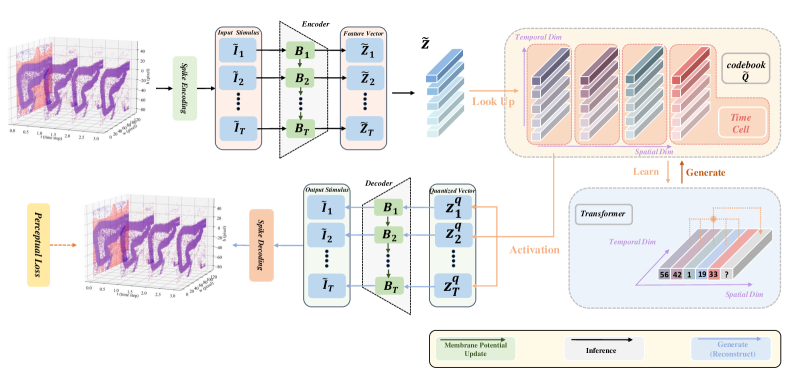
Figure 1: The overview of the proposed method. After spike encoding, the input stimulus $\tilde{I}_{t}$, is processed by the encoder to yield $z_{t}$. Concatenating $z_{t}$ and passing it through the temporal codebook $\tilde{Q}$ produces quantized $z^{q}_{t}$, which is then input to the decoder to reconstruct the stimulus $X_{t}$.

3.1 Leaky Integrate-and-Fire Model

We utilize the Leaky Integrate-and-Fire (LIF) neuron model [5] due to its simplicity and effectiveness in emulating the dynamic behavior of biological neurons. The discretized form of the LIF neuron dynamics is:

$$H[t]=V[t-1]+\frac{1}{\tau}(I[t]-(V[t-1]-V_{reset}))$$

$$S[t]=\Theta(H[t]-V_{th})$$ (1)

$$V[t]=H[t](1-S[t])+S[t]V_{reset}$$

Here, $\tau$ is the membrane time constant, $I[t]$ is the input synaptic current, $H[t]$ is the membrane potential after charging but before firing a spike, and $S[t]$ represents the spike generated when the membrane potential exceeds the threshold $V_{th}$, resetting the potential to $V_{reset}$. The Heaviside step function $\Theta(v)$ is 1 when $v\geq 0$ and 0 otherwise. Since $\Theta$ is non-differentiable, we have employed the surrogate gradient method [30] to optimize the SNN network.

3.2 Time Cell Inspired Temporal Codebook

In VQ-VAE, the codebook is essential for linking the encoder and decoder. It consists of discrete embedding vectors, each representing a unique quantized latent state. During encoding, the continuous latent representation is mapped to the nearest embedding vector in the codebook, typically based on Euclidean distance. Specifically, a static codebook $Q=\{q_{k}\}_{k=1}^{N_{q}}$ is employed, where $q_{k}\in\mathbb{R}^{c}$ and $N_{q}$ is the number of quantization vectors. For an input $\tilde{z}$, each $z_{t}$ is extracted and compared to $\{q_{k}\}$, selecting the quantized $z^{q}_{t}$ according to the minimum distance rule as shown in Eq. 2.

$$[z^{q}_{t}]_{ij}=\left(\operatorname*{arg\,min}_{q_{k}\in Q}||[z_{t}]_{ij}-q_{k}||\right)\in\mathbb{R}^{c}$$ (2)

where $[\cdot]_{ij}$ denotes the vector at the $i$-th row and $j$-th column of the tensor $z^{q}_{t}\in\mathbb{R}^{c\times h\times w}$. After obtaining $z^{q}$, $\tilde{z^{q}}$ is formed by concatenating $z^{q}_{t}$.

This process, known as vector quantization, discretizes the latent space, allowing the model to learn compressed representations of input data. The decoder reconstructs data from these quantized latent states. During training, the codebook is updated to ensure the embedding vectors capture essential features of the input, enhancing VQ-VAE’s generative capabilities. This mechanism enables VQ-VAE to sample from the discrete latent space to generate high-quality reconstructions and new samples.

While VQ-VAE shows promise in generative modeling, traditional implementations often struggle with temporal consistency in sequential data. The hippocampus, a critical brain region, encodes and retrieves temporal sequences, crucial for episodic memory formation. Its complex neural architecture supports a continuous temporal framework, integrating and recalling sequential experiences. Time cells, specialized neurons in the hippocampus, activate at specific moments within a sequence, encoding temporal aspects of experiences. These neurons are essential for maintaining the temporal structure of episodic memories, allowing the brain to distinguish between different time points and accurately reconstruct event sequences.

Inspired by the ability of hippocampal time cells to encode temporal information, we designed a temporal codebook $\tilde{Q}=\{\tilde{q}_{k}\}_{k=1}^{N_{q}}$, where each $\tilde{q}_{k}\in\mathbb{R}^{T\times c}$. Time cells provide a biological template for preserving temporal sequences, ensuring that events can be recalled in a coherent and temporally ordered manner. Our temporal codebook leverages this concept by incorporating time-sensitive embeddings to capture the dynamic changes in sequential data.

To retain temporal information in the quantized features, we use Equation 3 to calculate the quantized $\tilde{z^{q}}\in\mathbb{R}^{T\times c\times h\times w}$:

$$[\tilde{z^{q}}]_{ij}=\left(\operatorname*{arg\,min}_{q^{T}_{k}\in Q}||[\tilde{z^{q}}]_{ij}-\tilde{q}_{k}||\right)\in\mathbb{R}^{T\times c}$$ (3)

After obtaining $\tilde{z^{q}}$, the loss function for updating the temporal codebook can be derived as follows:

$$L_{Q^{T}}=||sg(\tilde{z})-\tilde{z^{q}}||^{2}_{2}+\beta||\tilde{z}-sg(\tilde{z^{q}})||^{2}_{2}$$ (4)

where $sg(\cdot)$ is the stop-gradient operator, and $\beta$ is a hyperparameter for weighting.

In $\tilde{Q}$, each vector $\tilde{q}_{k}\in\mathbb{R}^{T\times c}$ encompasses dimensions of temporal information $T$ and spatial information $h\times w$. Thus, this activation represents a spatiotemporal trajectory, akin to the activation of time cells, as illustrated in Figure 2.

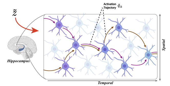
Figure 2: Spatiotemporal trajectories of neural activations from temporal codebook

3.3 Autoregressive Image Generation

For the image generation component, we adopt the approach proposed by [10], constructing an autoregressive language model using transformers [44]. We present both spiking and non-spiking versions of this model. The non-spiking version, based on a GPT-2-like structure with a 12-layer transformer, is employed for higher-quality image generation. The spiking version, incorporating LIF neurons and spiking self-attention mechanisms [24], is designed for better temporal correspondence and greater energy efficiency. This model generates new images by producing sequences of indices from the temporal codebook. The sequence of indices $s$ is modeled as:

$$P(s)=\prod_{i}P(s_{i}|s_{<i})$$ (5)

where $s_{i}$ represents the index at position $i$. The probability $P(s_{i}|s_{<i})$ is approximated by the autoregressive model driven by transformers, as illustrated in Figure 1. After obtaining the approximated index sequences $s$, we retrieve the corresponding approximated $\hat{\tilde{z_{q}}}$ from $Q^{T}$. Subsequently, through the reconstruction process, we generate the stimulus $\hat{X}=SD(D(\hat{\tilde{z_{q}}}))$.

3.4 Perceptual Quality Enhancement Using Generative Adversarial Training

To ensure high perceptual quality, we follow the methodology outlined in [10], utilizing perceptual loss [51] and a generative adversarial training process to guide the model’s loss and error propagation. Specifically, for the input stimulus $I$ and the reconstructed stimulus $X$, we extract features from both $I$ and $X$ using a pretrained VGG network. The perceptual loss is calculated based on the distance between the extracted features, as shown in Equation 6:

$$d(I,X)=\sum_{l}\frac{1}{H_{l}W_{l}}\sum_{h,w}||w_{l}\odot({f(I)}^{l}_{hw}-{f(X)}^{l}_{hw})||^{2}_{2}$$ (6)

where ${f(I)}^{l}\in\mathbb{R}^{H_{l}\times W_{l}\times C_{l}}$ and ${f(X)}^{l}\in\mathbb{R}^{H_{l}\times W_{l}\times C_{l}}$ are the features of $I$ and $X$ in the $l$-th layer of the pretrained VGG network. $w_{l}$ is a learnable scale factor representing the importance of each layer. In practice, we incorporate perceptual loss, vanilla MSE loss, and discriminator loss as metrics for error propagation.

4 Experiment

4.1 Setup

To validate our method’s efficacy, we conducted comprehensive experiments on various datasets. Standard benchmarks included MNIST, FashionMNIST, CIFAR10, CelebA, and downsampled LSUN Bedroom. For assessing the temporal codebook’s effectiveness in temporally correlated generative tasks, we used neuromorphic datasets NMNIST [33] and DVS-CIFAR10 [23]. Additionally, to demonstrate our method’s capability on high-resolution datasets, we selected $256\times 256$ resolution datasets CelebA-HQ [18], LSUN Bedroom, and LSUN Church [48]. The experiments were implemented using the BrainCog framework [49]. The base learning rate was set to $4.5\times 10^{-6}$ and adjusted according to batch size. AdamW was used as the optimizer, with the SNN time step varying from 2 to 6. The temporal codebook had $N_{q}=1024$ and each temporal step dimension $c=256$. We evaluated our model’s performance using Fréchet Inception Distance (FID) [14], Inception Score (IS) [36], Precision and Recall [35], and Kernel Inception Distance (KID) [3]. In Sections 4.2 and 4.3, we utilized the second-stage autoregressive model based on SNN. In other parts of the experiment, we employed the second-stage autoregressive model based on ANN. Notably, for the first-stage VQ-VAE model, we consistently used the SNN-based model through all experiments.

4.2 Comparative Analysis with SNN-based Generative Models

We conducted an extensive evaluation of our proposed method against other SNN-based generative models using the CelebA, CIFAR10, MNIST, FashionMNIST, and downsampled LSUN Bedroom datasets. The visual results of our method are illustrated in Figure 3. For quantitative assessment, we employed the FID across all datasets, and the IS for the CIFAR10 dataset. The comparative results, detailed in Table 1, demonstrate the superior performance of our model across various datasets. Notably, our model achieves superior results on all datasets except CIFAR10, where the FID score is marginally higher compared to the spiking diffusion models SDDPM and SDiT [6, 47]. However, our model still surpasses these models in terms of the Inception Score on CIFAR10, underscoring the effectiveness of our approach.

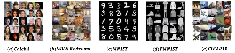
Figure 3: Comparative visualization of generated samples across various datasets

Dataset	Resolution	Model	Time Steps	IS $\uparrow$	FID $\downarrow$
CelebA∗	$64\times 64$	FSVAE [17]	16	3.70	101.60
		SGAD [11]	16	-	151.36
		SDDPM [6]	4	-	25.09
		Ours	4	-	13.11
LSUN Bedroom∗	$64\times 64$	SDDPM [6]	4	-	47.64
		Ours	6	-	12.97
MNSIT∗	$28\times 28$	FSVAE [17]	16	6.21	97.06
		SGAD [11]	16	-	69.64
		Spiking-Diffusion [25]	16	-	37.50
		SDDPM [6]	4	-	29.48
		SDiT [47]	4	2.45	5.54
		Ours	4	-	4.60
FashionMNIST∗	$28\times 28$	FSVAE [17]	16	4.55	90.12
		SGAD [11]	16	-	165.42
		Spiking-Diffusion [25]	16	-	91.98
		SDDPM [6]	4	-	21.38
		SDiT [47]	4	4.55	5.49
		Ours	4	-	3.67
CIFAR-10	$32\times 32$	FSVAE [17]	16	2.95	175.50
		SGAD [11]	16	-	181.50
		Spiking-Diffusion [25]	16	-	120.50
		SDDPM [6]	4	7.66	16.98
		SDiT [47]	4	4.08	22.17
		Ours	4	8.86	31.24

Table 1: Quantitative Comparison of Generative Models Across Multiple Datasets. (^∗ denotes the omission of Inception Score (IS) measurements, as this dataset bears little resemblance to ImageNet, rendering the IS metrics relatively nonsensical in this context)

4.3 Performance on Neuromorphic Datasets

To validate the effectiveness of our proposed method on neuromorphic datasets, we conducted experiments on the N-MNIST and DVS-CIFAR10 datasets. The results are illustrated in Figure 4. Figure 4(a) displays the temporal unfolding of the generated results on NMNIST [33], while Figure 4(b) shows the results on DVS-CIFAR10 [23]. It is evident that, compared to the vanilla codebook, the temporal codebook yields superior results both in terms of the quality of generation at individual time steps and in reducing temporal inconsistency.

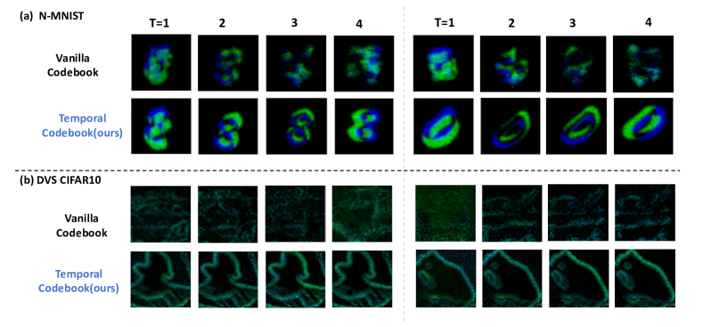
Figure 4: Temporal unfolding and generation quality comparison on neuromorphic datasets using temporal and vanilla codebooks on N-MNIST (a) and DVS-CIFAR10 (b).

4.4 High-Resolution Image Generation

To validate the performance of our method on high-resolution images, we conducted experiments on higher-resolution datasets, specifically the $256\times 256$ CelebA-HQ [18], LSUN Bedroom, and LSUN Church [48] datasets. Our study is the first to successfully employ SNNs for generating high-resolution images on the aforementioned datasets. We assessed the generated images using various metrics, including FID, Precision and Recall, and Kernel Inception Distance (KID), to provide a comprehensive evaluation and facilitate further research. The quantitative results are summarized in Table 2. The selections of generated samples are shown in Figure 5.

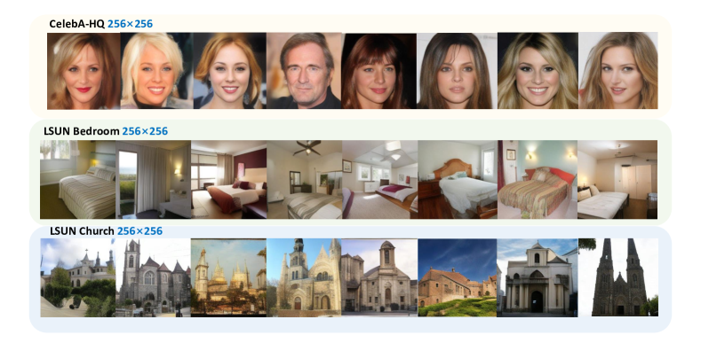
Figure 5: Generated high-resolution images using the proposed SNN-based method

Resolution	Dataset	FID $\downarrow$	Precision $\uparrow$	Recall $\uparrow$	KID $\downarrow$ ($\times 10^{-3}$)
256	CelebA-HQ	12.98	0.770	0.410	7.78
	LSUN Bedroom	6.61	0.630	0.405	3.98
	LSUN Church	6.62	0.675	0.465	3.22

Table 2: Quantitative evaluation metrics for high-resolution image generation

4.5 Effectiveness of the Temporal Codebook

In this section, we empirically demonstrate the significant impact of the temporal codebook on generation results. We first varied the time steps and measured the FID for two datasets, CelebA and LSUN Bedroom ($64\times 64$), employing both the temporal codebook and a vanilla codebook. The results are presented in Table 3.

Dataset	Codebook	FID $\downarrow$
		T=2	T=4	T=6
CelebA	Vanilla	28.00	67.39	73.09
	Temporal	14.87	13.57	13.69
LSUN Bedroom ($64\times 64$)	Vanilla	44.04	105.66	121.38
	Temporal	15.24	14.74	12.90

Table 3: Comparison of the FID between the temporal codebook and the vanilla codebook on the $64\times 64$ CelebA and LSUN Bedroom datasets.

The results reveal that the temporal codebook, enriched with temporal information, significantly enhances model performance compared to the vanilla codebook, highlighting the critical importance of temporal information in SNN-based generative models. Moreover, it is evident that increasing the time steps with the temporal codebook improves the FID, an effect not observed with the vanilla codebook. This further substantiates that the temporal codebook effectively integrates temporal information, and extending the time steps enables the model to generate images more accurately.

To further validate the effectiveness of the temporal codebook, we conducted a destructive experiment wherein vectors within the temporal codebook were randomly substituted with information from the last temporal steps. A temporal destruction factor $p_{d}$ was introduced to define the proportion of temporal information to be replaced with alternate temporal data. Visualizations for various values of $p_{d}$ are depicted in Figure 6. If $p_{d}=\frac{2}{6}$, it implies that out of a total of 6 time steps, 2 time steps are replaced with information from other time steps. The results indicate that at lower values of $p_{d}$, such as $p_{d}=\frac{1}{6}$ and $p_{d}=\frac{2}{6}$, the impact on image quality is minimal. However, as $p_{d}$ increases, there is a significant deterioration in image quality, particularly between $p_{d}=\frac{4}{6}$ and $p_{d}=\frac{5}{6}$.

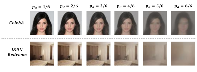
Figure 6: Effect of temporal destruction on image quality using temporal codebook. Visualizations for various values of $p_{d}$, the temporal destruction factor, show minimal impact on image quality at lower $p_{d}$ values, with significant deterioration observed at higher $p_{d}$ values.

We visualized the temporal codebook $\tilde{Q}$ by plotting a heatmap based on the magnitude of the elements in $\tilde{Q}$, as shown in Figure 7. The figure illustrates that as the time steps increase, the activity level of the corresponding elements in $\tilde{Q}$ decreases. This decreasing activity mirrors the behavior of biological time cells, which exhibit diminishing activity over a certain time interval after receiving a stimulus.

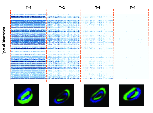
Figure 7: Visualization of the magnitude of elements in the temporal codebook $\tilde{Q}$

5 Conclusion

In this work, we introduced a novel SNN-based VQ-VAE framework that incorporates a temporal codebook inspired by hippocampal time cells. Our extensive experiments demonstrate the superior performance of our approach in generating high-quality, temporally consistent images across various datasets. Specifically, our method achieved state-of-the-art results on high-resolution datasets and showed significant improvements in temporal correlation and image quality compared to existing SNN-based generative models. We also validated the efficacy of the temporal codebook through destructive experiments, which underscored its crucial role in leveraging temporal information to enhance model performance. Our findings suggest that integrating temporal dynamics into the latent space of generative models holds great potential for advancing the field of neuromorphic computing and spiking neural networks. Future work will explore further optimizations and applications of this framework to other temporally rich generative tasks. However, there are some limitations to our approach. The complexity of the temporal codebook may increase computational burden. Future work will focus on optimizing this framework and exploring its applications to other temporally rich generative tasks.

References

- [1] Frederic Charles Bartlett. Remembering: A study in experimental and social psychology. Cambridge university press, 1995.
- [2] Phillip J Best, Aaron M White, and Ali Minai. Spatial processing in the brain: the activity of hippocampal place cells. Annual review of neuroscience, 24(1):459–486, 2001.
- [3] Mikołaj Bińkowski, Danica J Sutherland, Michael Arbel, and Arthur Gretton. Demystifying mmd gans. arXiv preprint arXiv:1801.01401, 2018.
- [4] Neil Burgess, Eleanor A Maguire, and John O’Keefe. The human hippocampus and spatial and episodic memory. Neuron, 35(4):625–641, 2002.
- [5] Anthony N Burkitt. A review of the integrate-and-fire neuron model: I. homogeneous synaptic input. Biological cybernetics, 95:1–19, 2006.
- [6] Jiahang Cao, Ziqing Wang, Hanzhong Guo, Hao Cheng, Qiang Zhang, and Renjing Xu. Spiking denoising diffusion probabilistic models. In Proceedings of the IEEE/CVF Winter Conference on Applications of Computer Vision, pages 4912–4921, 2024.
- [7] Rewon Child. Very deep vaes generalize autoregressive models and can outperform them on images. arXiv preprint arXiv:2011.10650, 2020.
- [8] Howard Eichenbaum. Time cells in the hippocampus: a new dimension for mapping memories. Nature Reviews Neuroscience, 15(11):732–744, 2014.
- [9] Howard Eichenbaum. The role of the hippocampus in navigation is memory. Journal of neurophysiology, 117(4):1785–1796, 2017.
- [10] Patrick Esser, Robin Rombach, and Bjorn Ommer. Taming transformers for high-resolution image synthesis. In Proceedings of the IEEE/CVF conference on computer vision and pattern recognition, pages 12873–12883, 2021.
- [11] Linghao Feng, Dongcheng Zhao, and Yi Zeng. Sgad: Spiking generative adversarial network with attention scoring decoding. arXiv preprint arXiv:2305.10246, 2023.
- [12] Tom M George, Kimberly L Stachenfeld, Caswell Barry, Claudia Clopath, and Tomoki Fukai. A generative model of the hippocampal formation trained with theta driven local learning rules. Advances in Neural Information Processing Systems, 36, 2024.
- [13] Demis Hassabis and Eleanor A Maguire. Deconstructing episodic memory with construction. Trends in cognitive sciences, 11(7):299–306, 2007.
- [14] Martin Heusel, Hubert Ramsauer, Thomas Unterthiner, Bernhard Nessler, and Sepp Hochreiter. Gans trained by a two time-scale update rule converge to a local nash equilibrium. Advances in neural information processing systems, 30, 2017.
- [15] Irina Higgins, Loic Matthey, Arka Pal, Christopher P Burgess, Xavier Glorot, Matthew M Botvinick, Shakir Mohamed, and Alexander Lerchner. beta-vae: Learning basic visual concepts with a constrained variational framework. ICLR (Poster), 3, 2017.
- [16] Jonathan Ho, Ajay Jain, and Pieter Abbeel. Denoising diffusion probabilistic models. Advances in neural information processing systems, 33:6840–6851, 2020.
- [17] Hiromichi Kamata, Yusuke Mukuta, and Tatsuya Harada. Fully spiking variational autoencoder. In Proceedings of the AAAI Conference on Artificial Intelligence, volume 36, pages 7059–7067, 2022.
- [18] Tero Karras, Timo Aila, Samuli Laine, and Jaakko Lehtinen. Progressive growing of gans for improved quality, stability, and variation. arXiv preprint arXiv:1710.10196, 2017.
- [19] Dhruv Khattar, Jaipal Singh Goud, Manish Gupta, and Vasudeva Varma. Mvae: Multimodal variational autoencoder for fake news detection. In The world wide web conference, pages 2915–2921, 2019.
- [20] Diederik P Kingma and Max Welling. Auto-encoding variational bayes. arXiv preprint arXiv:1312.6114, 2013.
- [21] Vineet Kotariya and Udayan Ganguly. Spiking-gan: a spiking generative adversarial network using time-to-first-spike coding. In 2022 International Joint Conference on Neural Networks (IJCNN), pages 1–7. IEEE, 2022.
- [22] Benjamin J Kraus, Robert J Robinson, John A White, Howard Eichenbaum, and Michael E Hasselmo. Hippocampal “time cells”: time versus path integration. Neuron, 78(6):1090–1101, 2013.
- [23] Hongmin Li, Hanchao Liu, Xiangyang Ji, Guoqi Li, and Luping Shi. Cifar10-dvs: an event-stream dataset for object classification. Frontiers in neuroscience, 11:244131, 2017.
- [24] Yudong Li, Yunlin Lei, and Xu Yang. Spikeformer: A novel architecture for training high-performance low-latency spiking neural network. arXiv preprint arXiv:2211.10686, 2022.
- [25] Mingxuan Liu, Rui Wen, and Hong Chen. Spiking-diffusion: Vector quantized discrete diffusion model with spiking neural networks. arXiv preprint arXiv:2308.10187, 2023.
- [26] Christopher J MacDonald, Kyle Q Lepage, Uri T Eden, and Howard Eichenbaum. Hippocampal “time cells” bridge the gap in memory for discontiguous events. Neuron, 71(4):737–749, 2011.
- [27] Joseph R Manns, Marc W Howard, and Howard Eichenbaum. Gradual changes in hippocampal activity support remembering the order of events. Neuron, 56(3):530–540, 2007.
- [28] Lisa Marshall and Jan Born. The contribution of sleep to hippocampus-dependent memory consolidation. Trends in cognitive sciences, 11(10):442–450, 2007.
- [29] David G Nagy, Balázs Török, and Gergő Orbán. Optimal forgetting: Semantic compression of episodic memories. PLoS Computational Biology, 16(10):e1008367, 2020.
- [30] Emre O Neftci, Hesham Mostafa, and Friedemann Zenke. Surrogate gradient learning in spiking neural networks: Bringing the power of gradient-based optimization to spiking neural networks. IEEE Signal Processing Magazine, 36(6):51–63, 2019.
- [31] John O’Keefe. Place units in the hippocampus of the freely moving rat. Experimental neurology, 51(1):78–109, 1976.
- [32] H Freyja Ólafsdóttir, Daniel Bush, and Caswell Barry. The role of hippocampal replay in memory and planning. Current Biology, 28(1):R37–R50, 2018.
- [33] Garrick Orchard, Ajinkya Jayawant, Gregory K Cohen, and Nitish Thakor. Converting static image datasets to spiking neuromorphic datasets using saccades. Frontiers in neuroscience, 9:159859, 2015.
- [34] Eva Pastalkova, Vladimir Itskov, Asohan Amarasingham, and Gyorgy Buzsaki. Internally generated cell assembly sequences in the rat hippocampus. Science, 321(5894):1322–1327, 2008.
- [35] Mehdi SM Sajjadi, Olivier Bachem, Mario Lucic, Olivier Bousquet, and Sylvain Gelly. Assessing generative models via precision and recall. Advances in neural information processing systems, 31, 2018.
- [36] Tim Salimans, Ian Goodfellow, Wojciech Zaremba, Vicki Cheung, Alec Radford, and Xi Chen. Improved techniques for training gans. Advances in neural information processing systems, 29, 2016.
- [37] Honi Sanders, Matthew A Wilson, and Samuel J Gershman. Hippocampal remapping as hidden state inference. Elife, 9:e51140, 2020.
- [38] Daniel L Schacter. Constructive memory: past and future. Dialogues in clinical neuroscience, 14(1):7–18, 2012.
- [39] Eleanor Spens and Neil Burgess. A generative model of memory construction and consolidation. Nature Human Behaviour, pages 1–18, 2024.
- [40] Larry R Squire. Memory and the hippocampus: a synthesis from findings with rats, monkeys, and humans. Psychological review, 99(2):195, 1992.
- [41] Arash Vahdat and Jan Kautz. Nvae: A deep hierarchical variational autoencoder. Advances in neural information processing systems, 33:19667–19679, 2020.
- [42] Gido M Van de Ven, Hava T Siegelmann, and Andreas S Tolias. Brain-inspired replay for continual learning with artificial neural networks. Nature communications, 11(1):4069, 2020.
- [43] Aaron Van Den Oord, Oriol Vinyals, et al. Neural discrete representation learning. Advances in neural information processing systems, 30, 2017.
- [44] Ashish Vaswani, Noam Shazeer, Niki Parmar, Jakob Uszkoreit, Llion Jones, Aidan N Gomez, Łukasz Kaiser, and Illia Polosukhin. Attention is all you need. Advances in neural information processing systems, 30, 2017.
- [45] James CR Whittington, Timothy H Muller, Shirley Mark, Guifen Chen, Caswell Barry, Neil Burgess, and Timothy EJ Behrens. The tolman-eichenbaum machine: unifying space and relational memory through generalization in the hippocampal formation. Cell, 183(5):1249–1263, 2020.
- [46] Mike Wu and Noah Goodman. Multimodal generative models for scalable weakly-supervised learning. Advances in neural information processing systems, 31, 2018.
- [47] Shu Yang, Hanzhi Ma, Chengting Yu, Aili Wang, and Er-Ping Li. Sdit: Spiking diffusion model with transformer. arXiv preprint arXiv:2402.11588, 2024.
- [48] Fisher Yu, Yinda Zhang, Shuran Song, Ari Seff, and Jianxiong Xiao. Lsun: Construction of a large-scale image dataset using deep learning with humans in the loop. arXiv preprint arXiv:1506.03365, 2015.
- [49] Yi Zeng, Dongcheng Zhao, Feifei Zhao, Guobin Shen, Yiting Dong, Enmeng Lu, Qian Zhang, Yinqian Sun, Qian Liang, Yuxuan Zhao, et al. Braincog: A spiking neural network based, brain-inspired cognitive intelligence engine for brain-inspired ai and brain simulation. Patterns, 4(8), 2023.
- [50] Junhai Zhai, Sufang Zhang, Junfen Chen, and Qiang He. Autoencoder and its various variants. In 2018 IEEE international conference on systems, man, and cybernetics (SMC), pages 415–419. IEEE, 2018.
- [51] Richard Zhang, Phillip Isola, Alexei A Efros, Eli Shechtman, and Oliver Wang. The unreasonable effectiveness of deep features as a perceptual metric. In Proceedings of the IEEE conference on computer vision and pattern recognition, pages 586–595, 2018.
- [52] Shengjia Zhao, Jiaming Song, and Stefano Ermon. Infovae: Information maximizing variational autoencoders. arXiv preprint arXiv:1706.02262, 2017.