Counterexamples to the $p(t)$-adic Littlewood Conjecture Over Small Finite Fields

Abstract

In 2004, de Mathan and Teulié stated the $p$-adic Littlewood Conjecture ($p$-$LC$) in analogy with the classical Littlewood Conjecture. Given a field $\mathbb{K}$ and an irreducible polynomial $p(t)$ with coefficients in $\mathbb{K}$, $p$-$LC$ admits a natural analogue over function fields, abbreviated to $p(t)$-$LC$ (and to $t$-$LC$ when $p(t)=t$).

In this paper, an explicit counterexample to $p(t)$-$LC$ is found over fields of characteristic 5. Furthermore, it is conjectured that this Laurent series disproves $p(t)$-$LC$ over all fields of characteristic $p\equiv 1\mod 4$. This fills a gap left by a breakthrough paper from Adiceam, Nesharim and Lunnon (2022) in which they conjecture $t$-$LC$ does not hold over all complementary fields of characteristic $p\equiv 3\mod 4$ and proving this in the case $p=3$. Supported by computational evidence, this provides a complete picture on how $p(t)$-$LC$ is expected to behave over all fields with characteristic not equal to 2. Furthermore, the counterexample to $t$-$LC$ over fields of characteristic 3 found by Adiceam, Nesharim and Lunnon is proven to also hold over fields of characteristic 7 and 11, which provides further evidence to the aforementioned conjecture.

Following previous work in this area, these results are achieved by building upon combinatorial arguments and are computer assisted. A new feature of the present work is the development of an efficient algorithm (implemented in Python) that combines the theory of automatic sequences with Diophantine approximation over function fields. This algorithm is expected to be useful for further research around Littlewood-type conjectures over function fields.

1 Introduction

Let $\alpha$ be a real number and let $|\alpha|$ denote its usual absolute value. Define the distance to the nearest integer of $\alpha$ as $|\langle\alpha\rangle|=\min_{n\in\mathbb{Z}}\{|\alpha-n|\}$. The famous Littlewood Conjecture (1930’s) states that for any pair of real numbers $(\alpha,\beta)$,

$$\liminf_{n\to\infty}|n|\cdot|\langle n\alpha\rangle|\cdot|\langle n\beta\rangle|=0$$ (1.1)

From now on, “Littlewood’s Conjecture” is abbreviated to $LC$. In 2006, Einsiedler, Katok and Lindenstrauss [EKL06] proved that the set of counterexamples to (1.1) has Hausdorff dimension equal to zero. This remains the most significant progress to date towards proving $LC$. In 2004, de Mathan and Teulié [MT04] formulated a similar conjecture that has become known as the $p$-adic Littlewood Conjecture ($p$-$LC$). Recall that, for a given prime $p$ and natural number $n$, the $p$-adic norm of $n$ is defined as

$$|n|_{p}=p^{-\nu_{p}(n)},\leavevmode\nobreak\ \leavevmode\nobreak\ \text{ where }\leavevmode\nobreak\ \leavevmode\nobreak\ \nu_{p}(n):=\max_{i\in\mathbb{N}}\{i:p^{i}|n\}.$$ (1.2)

Conjecture 1.1 ($p$-$LC$, de Mathan and Teulié, 2004).

For any real number $\alpha$ and any prime $p$,

$$\inf_{n\in\mathbb{N}\backslash\{0\}}|n|\cdot|n|_{p}\cdot|\langle n\alpha\rangle|=0.$$ (1.3)

Similarly to $LC$, Einsiedler and Kleinbock [EK07] proved in 2007 that the set of counterexamples to $p$-$LC$ has Hausdorff dimension equal to zero. For a deeper exploration of $LC$ and $p$-$LC$, see [BBEK15, Bug14, Bug09] and [Que09]. Both of the aforementioned conjectures admit natural counterparts over function fields sitting over a ground field $\mathbb{K}$, with the focus of this paper being on the analogue of $p$-$LC$. Since the analogues of $LC$ and $p$-$LC$ are known to be false when $\mathbb{K}$ is infinite (see [Bad21, BM08] and [MT04]), it is assumed throughout this paper that the ground field $\mathbb{K}$ is finite.

Let then $\mathbb{K}=\mathbb{F}_{q}$ be the finite field with cardinality $q$. Denote the ring of polynomials with coefficients in $\mathbb{F}_{q}$ as $\mathbb{F}_{q}[t]$ and let $\mathbb{F}_{q}(t)$ be the field of rational functions. The norm of $\Theta(t)\in\mathbb{F}_{q}(t)$ is defined as

$$|\Theta(t)|=q^{\deg(\Theta(t))}.$$ (1.4)

This metric is used to define the completion of $\mathbb{F}_{q}(t)$, namely the field of formal Laurent series

$$\mathbb{F}_{q}((t^{-1}))=\left\{\sum_{i=-h}^{\infty}a_{i}t^{-i}:h\in\mathbb{Z}\text{ and }a_{i}\in\mathbb{F}_{q}\right\}.$$

In the function field set up, the analogue of a prime number is an irreducible polynomial $p(t)\in\mathbb{F}_{q}[t]$. Similarly to (1.2), define the $p(t)$-adic norm of a polynomial $N(t)\in\mathbb{F}_{q}[t]$ as

$$|N(t)|_{p(t)}=|p(t)|^{-\nu_{p(t)}(N(t)},\leavevmode\nobreak\ \leavevmode\nobreak\ \text{ where }\leavevmode\nobreak\ \leavevmode\nobreak\ \nu_{p(t)}(N(t))=\max_{i\in\mathbb{N}}\{i:p(t)^{i}|N(t)\}.$$

The analogue of $p$-$LC$, called the $p(t)$-adic Littlewood Conjecture ($p(t)$-$LC$), is then:

Conjecture 1.2 ($p(t)$-$LC$).

Let $\mathbb{F}_{q}$ be a finite field. For every $\Theta(t)$ in $\mathbb{F}_{q}((t^{-1}))$ and every irreducible $p(t)$ in $\mathbb{F}_{q}[t]$,

$$\inf_{\mathbb{N}(t)\in\mathbb{F}_{q}[t]\backslash\{0\}}|N(t)|\cdot|N(t)|_{p(t)}\cdot|\langle N(t)\cdot\Theta(t)\rangle|=0.$$

When $p(t)=t$, $p(t)$-$LC$ is further abbreviated to $t$-$LC$.

Not all results about $p$-$LC$ translate into the positive characteristic set up. In 2020, Einsiedler, Lindenstrauss and Mohammadi [ELM17] provided the function field analogues of the measure classification results of both Lindenstrauss, Einsiedler and Katok [EKL06] and Einsiedler and Kleinbock [EK07]. However, it is not clear if these results are sufficient for proving anything about the Hausdorff dimension of the set of counterexamples to $p(t)$-$LC$. The most significant progress towards testing the validity of Conjecture 1.2 is due to a breakthrough paper by Adiceam, Nesharim and Lunnon [ANL21] that provided an explicit counterexample to $t$-$LC$ over fields of characteristic three. The coefficients of this Laurent series, denoted $\Upsilon(t)$, is the Paperfolding sequence. Whilst the Paperfolding sequence has been studied extensively (it corresponds to the $n=1$ case of Definition 1.3 below), the larger family of $n^{\textup{th}}$-Level Paperfolding sequences introduced hereafter is original to this paper. It serves to unify the counterexample to $p(t)$-$LC$ found in [ANL21] with the results in this paper.

Definition 1.3.

Let $n$ be a natural number, $\nu_{p}(n)$ be as in (1.2) and let $\overline{\leavevmode\nobreak\ \cdot\leavevmode\nobreak\ }$ be the value of the input modulo $2^{n+1}$. Define the $n^{\textup{th}}$-Level Paperfolding Sequence $(\Pi_{i}^{(n)})_{i\geq 1}$ as

$$\Pi^{(n)}_{i}=\frac{\overline{2^{-\nu_{2}(i)}i}-1}{2}\cdotp$$ (1.5)

Computer evidence provided by Adiceam, Nesharim and Lunnon [ANL21] provides strong support for the following conjecture:

Conjecture 1.4 (Adiceam, Nesharim, Lunnon).

Let $p\equiv 3\mod 4$ be a prime. Then, $\Upsilon(t)$ is a counterexample to $t$-$LC$ over fields of characteristic $p$.

The same computations nevertheless show that it is extremely unlikely that $\Upsilon(t)$ should provide a counterexample to $t$-$LC$ in the complementary case when the ground field has characteristic $p\equiv 1\mod 4$. The following theorem fills this gap.

Theorem 1.5.

Let $\Xi(t)\in\mathbb{F}_{5}((t^{-1}))$ be a Laurent series whose coefficients are given by the second-level Paperfolding sequence $(\Pi^{(2)}_{n})_{n\geq 0}$ as in Definition 1.3. Then $\Xi(t)$ is a counterexample to $t$-$LC$ over fields of characteristic 5.

Since $\mathbb{F}_{p}$ is a subfield of $\mathbb{F}_{p^{n}}$ for any natural number $n$, it is a simple corollary of Theorem 1.5 that $t$-$LC$ fails over any finite field of characteristic 5 (see [ANL21, 4] for details).

Not only do the First and Second Level Paperfolding Sequences provide counterexamples to $t$-$LC$, but they also induce counterexamples to $p(t)$-$LC$ for any irreducible polynomial $p(t)$. This is due to the following result by the second named author [Rob23].

Theorem 1.6.

Let $p(t)\in\mathbb{K}[t]$ be an irreducible polynomial of degree $m$ and let $l$ be a positive integer. Any counterexample to $t$-$LC$ induces a counterexample to $p(t)$-$LC$ in the following sense: if $\Theta(t)=\sum_{i=1}^{\infty}a_{i}t^{-i}\in\mathbb{K}((t^{-1}))$ satisfies

$$\inf_{\mathbb{N}(t)\in\mathbb{F}_{q}[t]\backslash\{0\}}|N(t)|\cdot|N(t)|_{t}\cdot|\langle N(t)\cdot\Theta(t)\rangle|=q^{-l},$$

then $\Theta(p(t))=\sum_{i=1}^{\infty}a_{i}p(t)^{-i}\in\mathbb{K}((t^{-1}))$ satisfies

$$\inf_{\mathbb{N}(t)\in\mathbb{F}_{q}[t]\backslash\{0\}}|N(t)|\cdot|N(t)|_{p(t)}\cdot|\langle N(t)\cdot\Theta(t)\rangle|=q^{-lm}.$$

Applying Theorem 1.6 to $\Xi(t)$ immediately results in the following corollary:

Corollary 1.7.

Let $q$ be a positive power of $5$, let $p(t)\in\mathbb{F}_{q}[t]$ be an irreducible polynomial and let $(\Pi^{(2)}_{i})_{i\geq 1}$ be as in Definition 1.3. Then, the Laurent series

$$\Xi(p(t)):=\sum_{i=1}^{\infty}\Pi^{(2)}_{i}p(t)^{-i}$$

disproves $p(t)$-$LC$ over $\mathbb{F}_{q}$.

Complementing Conjecture 1.4, strong computational evidence suggests that $\Xi(p(t))$ does not satisfy $p(t)$-$LC$ over any field of characteristic $p\equiv 1\mod 4$. Therefore, the Second-Level Paperfolding Sequence is significant not only due to Theorem 1.7, but also from the fact that it provides a complete picture of how $p(t)$-$LC$ fails over any finite field of odd characteristic. As a consequence, one can conjecture on the failure of $p(t)$-$LC$ over all finite fields with odd characteristic. The complementary case where the finite field has even characteristic is more mysterious. In Section 5, computational evidence is provided that suggests that $t$-$LC$ is true over $\mathbb{F}_{2}$. The following conjecture summarises the expected behaviour of $t$-$LC$ in the cases discussed thus far.

Conjecture 1.8.

Let $p$ be a prime and let $\mathbb{K}$ be a field of characteristic $p$.

1. If $p=2$ and $\mathbb{K}=\mathbb{F}_{2}$, then $p(t)$-$LC$ is true for every irreducible $p(t)\in\mathbb{F}_{2}[t]$.

2. If $p\equiv 1\mod 4$, then the First Level Paperfolding Sequence is a counterexample to $p(t)$-$LC$ over $\mathbb{K}$.

3. If $p\equiv 3\mod 4$, then the Second Level Paperfolding Sequence is a counterexample to $p(t)$-$LC$ over $\mathbb{K}$.

Until now, the only evidence for Statement 3 of Conjecture 1.8 was provided by Adiceam, Nesharim and Lunnon in [ANL21]. To remedy this, the method used to prove Theorem 1.7 is also applied to the Paperfolding Laurent series $\Upsilon(t)$ to disprove $t$-$LC$ in fields of characteristic 7 and 11. Combined with Theorem 1.6, this yields the following result:

Theorem 1.9.

Let $q$ be a positive power of $7$ or $11$, let $p(t)\in\mathbb{F}_{q}[t]$ be an irreducible polynomial and let $(\Pi^{(1)}_{i})_{i\geq 1}$ be as in Definition 1.3. Then the Laurent series

$$\Upsilon(p(t)):=\sum_{i=1}^{\infty}\Pi^{(1)}_{i}p(t)^{-i}$$

is a counterexample to $p(t)$-$LC$ over $\mathbb{F}_{q}$.

The proofs of Theorems 1.7 and 1.9 are achieved by rephrasing $t$-$LC$ () in terms of the so-called Number Wall of a sequence, which is defined in Section 2. For the purposes of this introduction, the number wall of a one dimensional sequence $S$ is a two dimensional sequence derived entirely from $S$. The core idea used to prove Theorems 1.7 and 1.9 is similar to that used by Adiceam, Nesharim and Lunnon in [ANL21]. That is, the number wall is shown to be the limiting sequence of a 2-morphism applied to a finite set of tiles. Both the 2-morphism and the tiles are provided explicitly. The implementation of their algorithm can be found at [Lun17] and [Nes]. Theoretically, the algorithm used in [ANL21] could be used to obtain Theorems 1.7 and 1.9. However, the time it would take to do so is not manageable, in any way.

In this paper, two key improvements are made that allow for the proof of Theorems 1.7 and 1.9 with a much shorter runtime. Firstly, the shape of the tiles used has been changed from [ANL21], decreasing the amount required to cover the number wall of the First Level Paperfolding sequence over $\mathbb{F}_{3}$ by a large order of magnitude. Furthermore, a new tiling algorithm has been created that foregoes the need to generate large portions of the number wall under consideration, allowing for savings in both time and memory. This is the main contribution to the computing aspect of the new and growing theory of number walls. The authors believe this algorithm will be needed for future developments occurring in this area of research. This is discussed further in Section 5. See [RG] for the codebase.

The paper is organised as follows. Section 2 introduces the concept of the number wall and provides the key results needed for the proof of Theorems 1.7 and 1.9. Central to these results is the theory of automatic sequences: Section 3 focuses on this and discusses how the automaticity of a sequence is reflected in its number wall. The proof of both Theorem 1.7 and Theorem 1.9 is computer assisted and the algorithm used is provided in Section 4, with details of the implementation of this code into Python found in Appendix A. Finally, further open problems and conjectures are stated in Section 5.

Acknowledgements

The second named author is grateful to his supervisor Faustin Adiceam for his insight, support and supervision for the duration of this project. The same author acknowledges the financial support of the Heilbronn Institute. Finally, the authors would like to acknowledge the assistance given by Research IT and the use of the Computational Shared Facility at The University of Manchester.

2 The Correspondence Between $p(t)$-$LC$ and Number Walls

The following definition is central to the study of number walls.

Definition 2.1.

A matrix $(s_{i,j})$ for $0\leq i\leq n,0\leq j\leq m$ is called Toeplitz if all the entries on a diagonal are equal. Equivalently, $s_{i,j}=s_{i+1,j+1}$ for any $n\in\mathbb{N}$ such that this entry is defined.

Given a doubly infinite sequence $S:=(s_{i})_{i\in\mathbb{Z}}$, natural numbers $m$ and $v$, and an integer $n$, define the $(m+1)\times(v+1)$ Toeplitz matrix $T_{S}(n,m,v):=(s_{i-j+n})_{0\leq i\leq m,0\leq j\leq v}$ as

$$T_{S}(n,m,v):=\begin{pmatrix}s_{n}&s_{n+1}&\dots&s_{n+v}\\ s_{n-1}&s_{n}&\dots&s_{n+v-1}\\ \vdots&&&\vdots\\ s_{n-m}&s_{n-m+1}&\dots&s_{n-m+v}\end{pmatrix}$$

If $v=m$, this is abbreviated to $T_{S}(n,m)$. The Laurent series $\Theta(t)=\sum^{\infty}_{i=1}s_{i}t^{-1}\in\mathbb{F}_{q}((t^{-1}))$ is identified to the sequence $S=(s_{i})_{i\geq 1}$. Accordingly, let $T_{\Theta}(n,m,v)=T_{S}(n,m,v)$.

Definition 2.2.

Let $S=(s_{i})_{i\in\mathbb{Z}}$ be a doubly infinite sequence over a finite field $\mathbb{F}_{q}$. The number wall of the sequence $S$ is defined as the two dimensional array of numbers $W_{q}(S)=(W_{q,m,n}(S))_{n,m\in\mathbb{Z}}$ with

$$W_{q,m,n}(S)=\begin{cases}\det(T_{S}(n,m))&\textup{ if }m\geq 0,\\ 1&\textup{ if }m=-1,\\ 0&\textup{ if }m<-1.\end{cases}$$

In keeping with standard matrix notation, $m$ increases as the rows go down the page and $n$ increases from left to right. The remainder of this section only mentions results crucial for this paper. For a more comprehensive look at number walls, see [ANL21, Section 3],[CG95, pp 85-89], [Lun09, Rob23] and [Lun01].

A key feature of number walls is that the zero entries can only appear in specific shapes:

Theorem 2.3 (Square Window Theorem).

Zero entries in a Number Wall can only occur within windows; that is, within square regions with horizontal and vertical edges.

Proof.

See [Lun01, p9]. ∎

Theorem 2.3 implies that the border of a window is always the boundary of a square with nonzero entries. This motivates the following definition:

Definition 2.4.

The entries of a number wall surrounding a window are referred to as the inner frame. The entries surrounding the inner frame form the outer frame.

The entries of the inner frame are extremely well structured:

Theorem 2.5.

The inner frame of a window with side length $l\geq 1$ is comprised of 4 geometric sequences. These are along the top, left, right and bottom edges and they have ratios $P,Q,R$ and $S$ respectively with origins at the top left and bottom right. Furthermore, these ratios satisfy the relation

$$\frac{PS}{QR}=(-1)^{l}.$$

Proof.

See [Lun01, p11]. ∎

See Figure 1 for an example of a window of side length $l$. For $i\in\{0,\dots,l+1\}$, the inner and outer frames are labelled by the entries $A_{i},B_{i},C_{i},D_{i}$ and $E_{i},F_{i},G_{i},H_{i}$ respectively. The ratios of the geometric sequences comprising the inner frame are labelled as $P,Q,R$ and $S$.

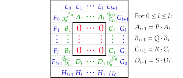
Figure 1: Illustration of a window in a number wall. The window, inner frame and outer frame are in red, green and blue, respectively.

Calculating a number wall from its definition is a computationally exhausting task. The following theorem gives a simple and far more efficient way to calculate the $m^{\textup{th}}$ row using the previous rows.

Theorem 2.6 (Frame Constraints).

Given a doubly infinite sequence $S=(s_{i})_{i\in\mathbb{Z}}$, the number wall $(W_{q,m,n})_{n,m\in\mathbb{Z}}:=(W_{q,m,n}(S))_{n,m\in\mathbb{Z}}$ can be generated by a recurrence in row $m\in\mathbb{Z}$ in terms of the previous rows. More precisely, with the notation of Figure 1,

$$W_{q,m,n}=\begin{cases}\begin{aligned} &0&&\textup{ if }m<-1\textup{ or if }(m,n)\textup{ is within a window;}&\\ &1&&\textup{ if }m=-1;&\\ &s_{n}&&\textup{ if }m=0;&\\ &\frac{W_{q,m-1,n}^{2}-W_{q,m-1,n-1}W_{q,m-1n+1}}{W_{q,m-2,n}}&&\textup{ if }m>0\textup{ and }W_{q,m-2,n}\neq 0;&\\ &D_{k}=\frac{(-1)^{l\cdot k}B_{k}C_{k}}{A_{k}}&&\textup{ if }m>0\textup{ and }W_{q,m-2,n}=0=W_{q,m-1,n};&\\ &H_{k}=\frac{\frac{QE_{k}}{A_{k}}+(-1)^{k}\frac{PF1_{k}}{B_{k}}-(-1)^{k}\frac{SG_{k}}{C_{k}}}{R/D_{k}}&&\textup{ if }m>0\textup{ and }W_{q,n,m-2}=0\neq W_{q,n,m-1}.&\end{aligned}\end{cases}$$

Proof.

See [Lun01, p11] ∎

The value of $k$ above is found in the natural way from the value of $m,n$ and the side length $l$. The final three equations above are known as the First, Second and Third Frame Constraint Equations. These allow the number wall of a sequence to be considered independently of its original definition in terms of Toeplitz matrices. It is simple to see that a finite sequence of length $r$ generates a number wall in the shape of an isosceles triangle with depth $\left\lfloor\frac{r-1}{2}\right\rfloor$. If $S$ is a finite sequence in $\mathbb{F}_{q}$, then denote the finite number wall of $S$ as $W_{q}(S)$. To make number walls visually accessible, each entry is given a unique colour depending on its value (See Figure 2).

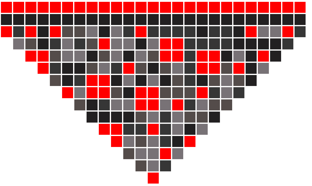
Figure 2: The number wall of a sequence of length 25 generated uniformly and randomly over $\mathbb{F}_{5}$. The zero entries are coloured in red, with the nonzero values assigned a shade of grey, with 1 being the darkest and 4 being the lightest. The top row (red) has index $-2$. It is included as it initiates the recurrence relations given by Theorem 2.6 that are used to generate this image.

The following result from [ANL21, p5] rephrases the $t$-adic Littlewood conjecture in terms of number walls.

Lemma 2.7.

Let $\Theta(t)=\sum^{\infty}_{i=1}s_{i}t^{-i}\in\mathbb{F}_{q}((t^{-1}))$ be a Laurent series and $S=(s_{i})_{i\in\mathbb{N}}$ be the sequence of its coefficients. Then, $\Theta(t)$ is a counterexample to $t$-LC if and only if there exists an $l$ in the natural numbers such that the number wall of $(s_{i})_{i\geq 0}$ has no window of size larger than $l$.

Combining Lemma 2.7 with Theorem 1.6 reduces the proof of Theorems 1.7 and 1.9 to proving that the number wall of the First and the Second Level Paperfolding Sequences, over their respective finite fields, have bounded window size. These sequences are extremely structured, and the proof of Theorems 1.7 and 1.9 is achieved by proving their respective number walls inherit this structure. To formalise this idea, Section 3 introduces the concept of automatic sequences.

3 Detecting Automaticity in a Number Wall

This section only covers the basic properties of automatic sequences needed for this paper. See [AS03] for more on this theory.

Let $\Sigma$ be a finite alphabet and let $\Sigma^{*}$ be the set of all finite words made up from $\Sigma$, including the empty word. For $x,y\in\Sigma^{*}$, let $xy$ denote the concatenation of $y$ to the right side of $x$. A function $\phi:\Sigma^{*}\to\Sigma^{*}$ is called a morphism if $\phi(xy)=\phi(x)\phi(y)$ for any $x,y\in\Sigma^{*}$. Furthermore, let $L(w)$ denote the length of the word $w\in\Sigma^{*}$. If $k$ is a natural number, then $\phi$ is a $k$-morphism if $L(\phi(w))=k\cdot L(w)$ for any word $w$ in $\Sigma^{*}$.

An element of $\Sigma$ is called $\phi$-prolongable if it is the first letter of its own image under $\phi$. If a sequence $S=(s_{n})_{n\geq 0}$ is defined over $\Sigma$ and satisfies $\phi(S)=S$, then $s_{0}$ is $\phi$-prolongable and $S$ is a fixed point of $\phi$, denoted $\phi^{\omega}(s_{0})$. For a finite alphabet $\Delta$, a coding is a function $\tau:\Sigma\to\Delta$ which is a uniform 1-morphism. The notation $\tau(S)$ is shorthand for applying $\tau$ to each element of the sequence $S$. The following concept is at the heart of the proof of Theorems 1.7 and 1.9.

Definition 3.1.

Let $k$ be a natural number. An infinite sequence $S=(s_{n})_{n\geq 0}$ is called $k$-automatic if for each $n\geq 0$, $s_{n}$ can be derived from a finite state automaton which takes the base-$k$ digits of $n$ as an input.

For the purposes of this paper, the following theorem of Cobham [Cob72] (rephrased in modern language in [AS03, Theorem 6.3.2]) can be seen as an alternative definition for automatic sequences:

Theorem 3.2 (Cobham’s Theorem).

A sequence is $k$-automatic if and only if it is the fixed point of a uniform $k$-morphism.

The following example is central to this paper. The notation used below will be fixed for the duration of the paper.

Example 3.3.

Let $\Gamma=\{A,B,C,D\}$ be an alphabet and define the 2-morphism $\psi:\Gamma\to\Gamma^{*}$ as

$$\psi(A)=AB \psi(B)=CB \psi(C)=AD \psi(D)=CD.$$ (3.1)

Let $\Delta=\{0,1\}$. Then the First Level Paperfolding sequence can be constructed as $\pi(\phi^{\omega}(A))$, where $\pi:\Gamma\to\Delta$ is a coding defined by

$$\pi(A)=0 \pi(B)=0 \pi(C)=1 \pi(D)=1.$$ (3.2)

The coding generating a $k$-automatic sequence is not unique. For example, if $S$ is a $k$-automatic sequence generated by a $k$-morphism $\phi$ and a coding $\tau$ on a finite alphabet $\Sigma=\{\sigma_{0},\dots,\sigma_{n}\}$, one can define its $k$-compression by setting $\tau^{\prime}(\sigma_{i})=\tau(\phi(\sigma_{i}))$. Applying the $k$-compression $n$ times will be referred to as taking the $k^{n}$-compression.

Example 3.4.

The $2$-compression of the First Level Paperfolding sequence is given by the same 2-morphism $\phi$ as in (4.1) and by the coding $\pi^{\prime}$ defined as

$$\pi^{\prime}(A)=00 \pi^{\prime}(B)=10 \pi^{\prime}(C)=01 \pi^{\prime}(D)=11.$$

Applying the 2-compression again returns the 4-compression:

$$\pi^{\prime\prime}(A)=0010 \pi^{\prime\prime}(B)=0110 \pi^{\prime\prime}(C)=0011 \pi^{\prime\prime}(D)=0111.$$

3.1 The Number Wall of an Automatic Sequence

Let $\phi:\Sigma^{*}\to\Sigma^{*}$ be a $k$-morphism on the finite alphabet $\Sigma$, and let $s_{0}\in\Sigma$ be $\phi$-prolongable. Define $S=\tau(\phi^{\omega}(s_{0}))$ for a coding $\tau:\Sigma\to\Delta$, where $\Delta$ is a finite alphabet whose elements are finite sequences with entries in $\mathbb{F}_{q}$. If $k$ is even, it may be assumed without loss of generality that the coding $\tau(x)$ has even length for every $x\in\Sigma$. Indeed, if this is not the case, replace $\tau(x)$ with its $k$-compression.

The image of each $x\in\Sigma$ under $\tau$ forms a finite sequence to which is associated a finite number wall as in Figure 2. Rows with negative index are included to create horizontal symmetry, resulting in the following shape:

Figure 3: The shape of a finite number wall generated by $\tau(x)$ when $L(\tau(x))=8$. Each block represents an entry, with the dark blue representing the rows with index $m\leq-1$ and the longest row being the sequence given by $\tau(x)$.

Blocks of the number wall in the shape of Figure 3 are called tiles. Figure 4 depicts how a number wall is split into tiles. When $k$ is odd and $\tau(x)$ has odd length for any tile $x\in\Sigma$, the number wall is split into tiles as depicted in the right image of Figure 4. This paper only deals with $2$-morphisms, and hence the number wall will always be split into tiles as depicted by the left image of Figure 4.

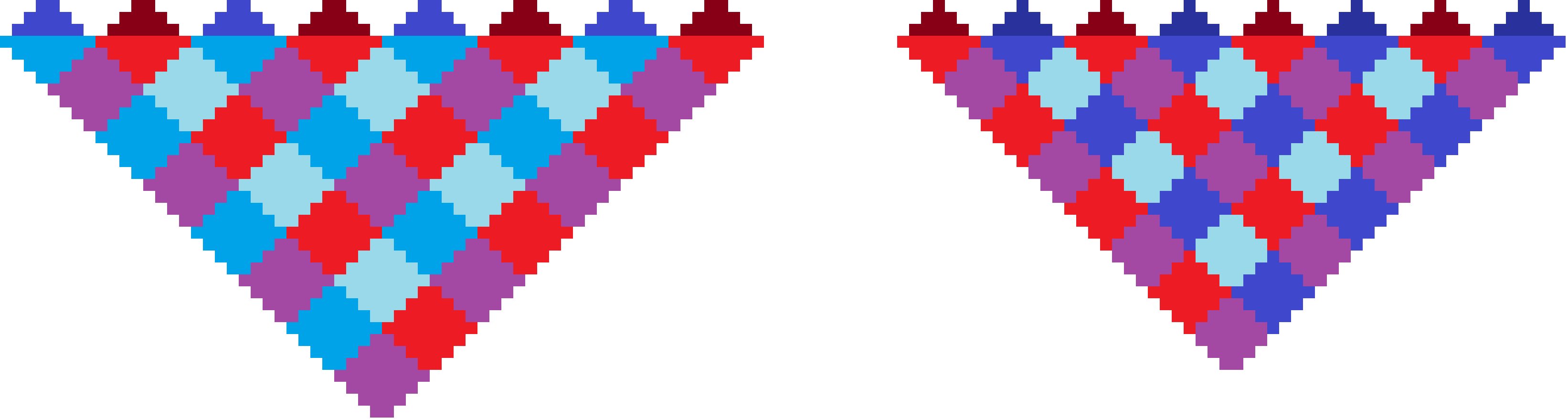
Figure 4: A large potion of the number wall split into tiles depending on if $\tau(x)$ has odd or even length. The dark red and blue show where the row index becomes negative. The remaining colours serve no other purpose than to distinguish one tile from another.

Each tile that contains part of the zeroth row of the number wall is associated to the element of $\Sigma$ that generates the tile when the coding is applied. Furthermore, each tile below the top row is associated to a subword of $\phi^{\omega}(A)$ by considering the tiles on the zeroth row of the number wall that generate it. For $r$ a non-negative integer, a tile of order $r$ is defined as any tile which is generated by exactly $r$ tiles on the zeroth row of the number wall. Hence, each tile of order $r$ is associated to a subword of $\phi^{\omega}(A)$ with length $r$.

Figure 5: The lowest outlined tile is associated to $ABA$, as this is the subword of $\phi^{\omega}(A)$ that appears above it. This tile is of order 3.

If $\phi$ is a $k$-morphism, $a,b$ are integers and $w$ is a finite word in $\Sigma^{*}$, define $\phi_{a,b}(w)$ as the subword $\phi(w)$ with the first $a$ letters and the last $b$ letters removed. Applying $\phi$ to the top row tiles induces a two-dimensional $k$-morphism $\Phi:\Sigma^{*}\to(\Sigma^{*})^{k^{2}}$ on subwords in $\Sigma^{*}$ given by

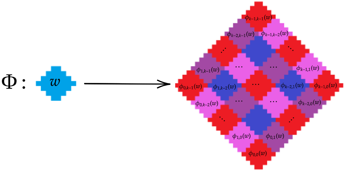
Figure 6: The two-dimensional $k$-morphism induced by $\phi$. Recall that every subword $w\in\Sigma^{*}$ corresponds to a tile made up of entries in the number wall, illustrated by Figure 5.

Every subword of $\phi^{\omega}(A)$ can be obtained by applying a sequence of $\phi_{a,b}$ to $A$. Applications of $\phi_{a,b}$ to any subword $w$ of length $l$ creates a subword of length $kl-a-b$. Hence, if $kl-a-b>l$, $\phi_{a,b}$ increases the length of the subword. Since $a+b\leq 2(k-1)$, this is always true when $l>2(k-1)$. In particular, applying $\phi_{a,b}$ such that $a+b=k-1$ to an entry of $\Sigma$ will return another entry of $\Sigma$, and $\phi_{k-1,k-1}$ applied to a subword of length 2 will return a subword of length 2. Applying $\phi_{a,b}$ such that $a+b>k$ to a subword of length 1 returns the empty word by definition.

As there are infinitely many finite subwords of $S$, and only finitely many possible tiles (as the entries of the number wall are in $\mathbb{F}_{q}$), there is no reason a priori that $\Phi$ should be a two-dimensional $k$-automatic sequence. That is, the pigeonhole principle implies there exists an infinite subset of $\Sigma^{*}$ whose elements are all associated to the same tile, yet may have different images under $\Phi$. The heart of the proof of Theorems 1.7 and 1.9 is in proving that, for the First and Second Level Paperfolding Sequences over the stated fields $\mathbb{F}_{q}$, $\Phi$ is indeed a two dimensional $k$-automatic sequence.

4 Explicit Morphism for the Number Wall of the First Level Paperfolding Sequence

Let $S$ be the First Level Paperfolding Sequence, let $\psi$ be the 2-morphism that generates it and let $\Psi$ be the induced 2-morphism on subwords illustrated by Figure 6. This section details the algorithm used to prove Theorem 1.9. That is, this algorithm finds an ordered finite alphabet $\Sigma=\Sigma_{S,p}$, a 2-morphism $\Phi=\Phi_{S,p}:\Sigma^{*}\to(\Sigma^{*})^{4}$, $\sigma_{0}\in\Sigma$ that is $\Phi$-prolongable, a set of tiles $T=T_{S,p}$ and a coding $\tau=\tau_{S,p}:\Sigma\to T$ such that $W_{p}(S)=\tau(\Phi^{\omega}(\sigma_{0}))$. The algorithm is almost identical when working with the Second Level Paperfolding Sequence to prove Theorem 1.7; the minor changes will be detailed at the end of this section. The proof is split into two main steps:

1. An efficient algorithm uses $\psi$ and the Frame Constraints (Theorem 2.6) to find the alphabet $\Sigma$, the two dimensional 2-morphism $\Phi$, the letter $\sigma_{0}$, the set of tiles $T$ and coding $\tau$.

2. That the two-dimensional sequence defined by ${\tau}({\Phi^{\omega}}({\sigma_{0}}))$ is proved equal to $W_{p}(S)$ by verifying that ${\tau}({\Phi^{\omega}}({\sigma_{0}}))$ satisfies the Frame Constraints (Theorem 2.6) and that the zeroth row is $S$.

Each step is split into two further sub-steps (1.1, 1.2, 2.1, and 2.2 below) and each sub-step is presented as its own algorithm. The steps of each algorithm are written in typewriter font and any necessary justification of each step is provided below in the normal font.

Part 1: Finding the Parameters

The algorithm begins with empty sets $\Sigma$ and $T$. As it progresses, letters (tiles, respectively) are added to $\Sigma$ (to $T$, respectively) and the 2-morphism $\Phi$ and coding $\tau$ are built. The finite alphabet ${\Sigma}$ will be comprised of letters $\sigma_{i}$, where $i$ is in a finite set $\{n\in\mathbb{Z}:-1\leq n\leq N\}$ for some $N<\infty$.

Algorithm 1.1: Initial Conditions

Let $\Gamma$, $\psi$ be as they were in Example 3.3 and define $\pi$ as the 8-compression of the coding from the same example. From now on, $\#T$ denotes the cardinality of a finite set $T$.

Step 1.1.1: The tile whose bottom row has index $-1$ is appended to ${T}$ and $\sigma_{-1}$ is appended to ${\Sigma}$.
Define $\tau(\sigma_{-1})$ as this tile. Similarly, the tile of all zeros is appended to $T$, $\sigma_{0}$ is appended
to $\Sigma$ and $\tau(\sigma_{0})$ is defined as this tile. These tiles are depicted in Figure 7.

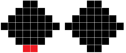
Figure 7: Left: The tile whose bottom row has index $-1$. The red entries are equal to 1, and the black entries are 0. Right: The tile of all zeros, with the same colour scheme.

Step 1.1.2: For each $\gamma\in\Gamma$, calculate the tile given by $W_{p}(\tau(\gamma))$ and append it to ${T}$. Each
time a tile is appended to ${T}$, append $\sigma_{m(T)}$ to ${\Sigma}$ where $m(T)=\#{T}-2$. Additionally, define ${\tau}(\sigma_{m(T)})=W_{p}(\tau(\gamma))$.

Note that a new letter is appended to ${\Sigma}$ whenever a new tile is discovered. Therefore, ${\tau}:\Sigma\to T$ is a bijection and hence its inverse is well defined.

When $k=2$, the image of $\sigma_{i}\in{\Sigma}$ under ${\Phi}$ is a 4-tuple $(\sigma_{i_{w}},\sigma_{i_{n}},\sigma_{i_{e}},\sigma_{i_{s}})$. Here, each entry of the 4-tuple has been associated to a cardinal direction (east, north, west, south) in the natural way. For any 4-tuple of tiles that are arranged as depicted in Figure 8, the scaffolding of the southern tile is defined as the 3-tuple given by the eastern, northern and western tiles.

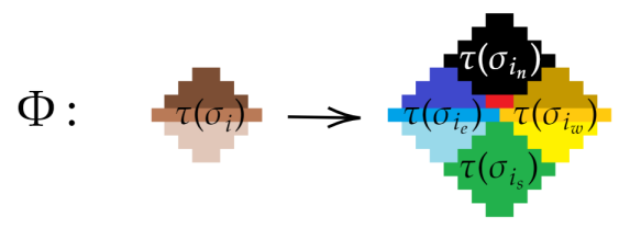
Figure 8: An illustration of $\Phi$ acting on a tile $\tau(\sigma_{i})$ which contains part of the zeroth row of the number wall. The black and red tile $\tau(\sigma_{-1})$ is the same as that from Figure 7. The middle row of the brown, blue and yellow tiles is made up from the zeroth row of the number wall. The lighter (darker, respectively) portions of these tiles have positive (negative, respectively) row index.

Step 1.1.3: Create an empty set $Scaf$. For each $\gamma\in\Gamma$, split $W_{p}(\tau(\psi(\gamma)))$ into 4 tiles as
depicted in Figure 8. The southern tile, denoted $t_{s}$, is appended to ${T}$ and $\sigma_{m(T)}$ is
appended to $\Sigma$. Append the scaffolding of $t_{s}$ to $Scaf$, and then define

$${\Phi}(\tau^{-1}(W_{p}(\pi(\gamma)))):=({\tau}^{-1}(W_{p}(\pi(\psi_{0,1}(\gamma)))),\leavevmode\nobreak\ \sigma_{-1},\leavevmode\nobreak\ {\tau}^{-1}(W_{p}(\pi(\psi_{1,0}(\gamma))),\leavevmode\nobreak\ \sigma_{m(T)}).$$

Step 1.1.4: For completeness, define $\Phi(\sigma_{-1})=(\sigma_{0},\sigma_{0},\sigma_{0},\sigma_{-1})$ and $\Phi(\sigma_{0})=(\sigma_{0},\sigma_{0},\sigma_{0},\sigma_{0})$.

Step 1.1.5: Return $Scaf$, ${T}$, ${\Sigma}$, ${\tau}$ and ${\Phi}$

At the end of Part 1.1, one has found all the tiles that make up the zeroth row of the number wall and the functions ${\Phi}$ and ${\tau}$ have been defined on these tiles. Furthermore, four second order tiles have been found by using the Frame Constraints (Theorem 2.6), and their scaffolding has been recorded.

Algorithm 1.2: Completing ${\Phi}$

Step 1.2.1: Let $\sigma_{l}$ be the first letter in ${\Sigma}$ such that ${\Phi}(\sigma_{l})$ is not yet defined. Let $\sigma_{i},\sigma_{j},\sigma_{k}\in{\Sigma}$ be the scaffolding of $\sigma_{l}$. Apply ${\Phi}$ to $\sigma_{i},\sigma_{j}$ and $\sigma_{k}$ to obtain the coloured parts of Figure 9.

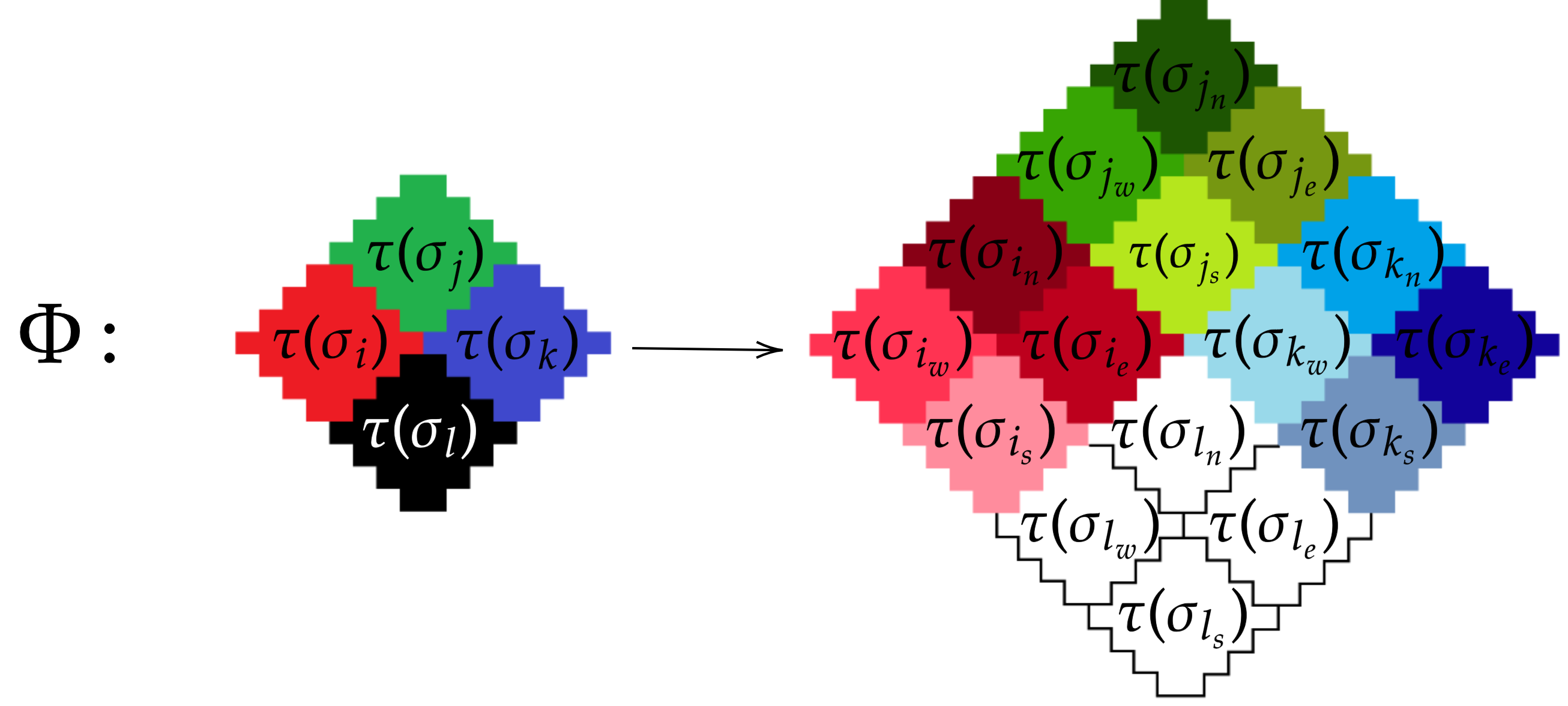
Figure 9: The result of applying ${\Phi}$ to the scaffolding of $\sigma_{l}$.

Step 1.2.2: Apply the Frame Constraints (Theorem 2.6) to calculate the tile $t={\tau}(\sigma_{l_{n}})$ in
Figure 9. If $t$ is not in ${T}$, append it, append $\sigma_{m(T)}$ to ${\Sigma}$ and append the scaffolding of $t$
to $Scaf$. Otherwise, do nothing.

If the number wall of the sequence $S$ contains windows of unbounded size, Step 1.2.2 will eventually fail. That is, the image of the scaffolding of $\sigma_{l}$ will not contain enough information to derive the white tiles in Figure 9.

Step 1.2.3: Define $\sigma_{l_{n}}:={\tau^{-1}}(t)$.

Step 1.2.4: Repeat steps 1.2.2 and 1.2.3 for ${\tau}(\sigma_{l_{w}})$, ${\tau}(\sigma_{l_{e}})$ and ${\tau}(\sigma_{l_{s}})$ in this order.

Processing tiles in the order north, west, east and south ensures that $\Phi$ is always defined on the scaffolding of $\sigma_{l}$ in Step 1.2.1.

Step 1.2.5: Define ${\Phi}(\sigma_{l})=(\sigma_{l_{w}},\sigma_{l_{n}},\sigma_{l_{e}},\sigma_{l_{s}})$.

Step 1.2.6: If there remains any $\sigma\in{\Sigma}$ whose image under ${\Phi}$ is undefined, go back to Step $1.2.1$.
Otherwise, return ${\Phi}$,${\Sigma}$, ${T}$, and ${\tau}$.

Algorithm 2.2 terminates when $\Phi(\sigma)$ has been defined for every $\sigma\in\Sigma$. This algorithm will eventually terminate, either because there are only finitely many possible tiles with entries in $\mathbb{F}_{q}$ or because the windows have grown too large and Step 1.2.2 fails. Assuming the algorithm has finished without failure, what is returned is a two dimensional automatic sequence given by $\Phi^{\omega}(\sigma_{1})$ and a coding $\tau$. Algorithms 2.1 and 2.2 verify that $\tau(\Phi^{\omega}(\sigma_{1}))=W_{p}(S)$.

Part 2: Verifying the 2-Morphism

The 2-morphism ${\Phi}$, the finite alphabet ${\Sigma}$, the tile set ${T}$ and the coding ${\tau}$ generate an automatic sequence. The next two algorithms serve to verify that this sequence is the number wall of $S$ modulo the chosen prime $p$. To achieve this, Algorithm 2.1 provides a way to find every possible combination of 4 tiles that can form a 4-tuple. That is, every combination of 4 tiles that can appear in the formation depicted in the left of Figure 9 or the right of Figure 8. Note, a 4-tuple does not have to be equal to $\Phi(\sigma)$ for some $\sigma\in\Sigma$ (See Figure 10). Algorithm 2.2 then verifies that each 4-tuple satisfies the Frame Constraints.

Algorithm 2.1: Finding all possible 4-tuples

Step 2.1.1: Define an empty set $Tup$ and for every $\sigma\in{\Sigma}$ append ${\Phi}(\sigma)$.

The set $Tup$ will contain every $4$-tuple that appears in $\Phi^{\omega}(\sigma_{1})$. Every such 4-tuple is contained in the image of some other 4-tuple under ${\Phi}$.

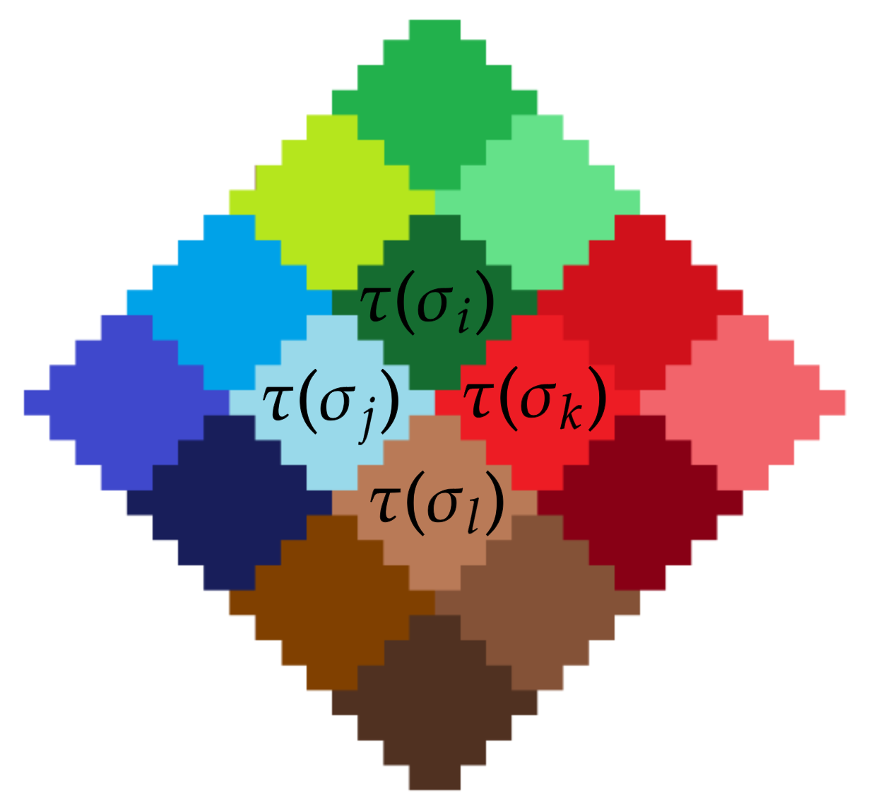
Figure 10: Each block of 4 tiles in a similar colour represent ${\tau}({\Phi}(\sigma))$ for some $\sigma\in{\Sigma}$. The 4-tuple of tiles $({\tau}(\sigma_{i}),{\tau}(\sigma_{j}),{\tau}(\sigma_{k}),{\tau}(\sigma_{l}))$ is contained within the image of these four $\sigma$ under ${\Phi}$.

Step 2.1.2: Let $\varsigma=\{\sigma_{i_{j}}:1\leq j\leq 4\}$ be the first 4-tuple in $Tup$ whose image has not yet been processed. Calculate the 16-tuple ${\Phi}(\varsigma)$.

Step 2.1.3: Check every possible 4-tuple contained within ${\Phi}(\varsigma)$. If it is not in $Tup$, append it to the end.

Note, there are nine such 4-tuples in total, but only five need to be checked because the four of them are images of some $\sigma\in{\Sigma}$ under ${\Phi}$ and hence are already in $Tup$.

Step 2.1.4: If the end of $Tup$ has been reached, return $Tup$. Otherwise, go back to step 2.1.1

When the end of the list is reached, this implies that set $Tup$ is closed under $\Phi$. That is, all the 4-tuples found when applying $\Phi$ to a 4-tuple in $Tup$ are already in $Tup$. In turn, this implies $Tup$ is a complete list.

Algorithm 2.2: Verifying the 4-tuples

The final step is to verify the 4-tuples satisfy the Frame Constraints. If they do, then this implies that $\tau(\Phi^{\omega}(\sigma_{1}))=W_{p}(S)$.

Step 2.2.1: Let $\varsigma$ be the first 4-tuple in $Tup$ that has not yet been processed by Algorithm 2.2. Apply ${\tau}$ to all entries of $\varsigma$ other than the southern one, denoted $\varsigma_{s}$.

Step 2.2.2:Let $\widetilde{\tau(\varsigma_{s})}$ be the tile calculated by applying the Frame Constraints (Theorem 2.6) to
the image of the scaffolding of $\varsigma_{s}$. If this is equal to ${\tau(\varsigma_{s})}$, move to Step 2.2.3. Otherwise,
return Failure

Step 2.2.3: If $\varsigma$ was the final 4-tuple in $Tup$, return $Tup$. Otherwise, go back to step $2.2.1$.

If Algorithm 2.2 is successful, then ${W_{p}(S)}$ is the number wall modulo $p$ of the sequence on its zeroth row. By construction, this sequence is the First Level Paperfolding sequence, and this completes the proof of automaticity. Furthermore, the if the windows had unbounded size then Step 1.2.2 would have failed, hence the First Level Paperfolding sequence provides a counterexample to the $t$-$LC$ over $\mathbb{F}_{p}$. Finally, applying Theorem 1.6 concludes the proof of Theorem 1.9.

The algorithm presented in this section remains virtually unchanged when applying it to the Second Level Paperfolding Sequence. The only differences in these cases is the $2$-morphism applied in Algorithm 1.1 and the size of the tiles, which need to be 16 entries long in their largest row. The $2$-morphism that generates the Second Level Paperfolding Sequence is given by Example 4.1. The proof is omitted. Indeed, a skeptical reader can consider the 2-morphism given in Example 4.1 below to be the definition of the Second Level Paperfolding Sequence since the algorithms in Section 4 are implemented without the use of equation (1.3).

Example 4.1.

Let $\Lambda=\{A,B,C,D,E,F,G,H,I,J,K,L\}$ be an alphabet and define the 2-morphism $\chi:\Lambda\to\Lambda^{*}$ as

$$\chi(A)=AB \chi(B)=CD \chi(C)=EF \chi(D)=GD \chi(E)=AH \chi(F)=CI$$

$$\chi(G)=EJ \chi(H)=CK \chi(I)=GI \chi(J)=CL \chi(K)=GK \chi(L)=GL.$$

Let $\Delta=\{0,1\}$. Then the Second Level Paperfolding Sequence can be constructed as $\upsilon(\chi^{\omega}(A))$, where $\upsilon:\Lambda\to\Delta$ is the coding defined by

$$\upsilon(A)=0 \upsilon(B)=0 \upsilon(C)=1 \upsilon(D)=0 \upsilon(E)=2 \upsilon(F)=1$$

$$\upsilon(G)=3 \upsilon(H)=2 \upsilon(I)=1 \upsilon(J)=3 \upsilon(K)=2 \upsilon(L)=3.$$

4.1 Results and Data

This section details the outcome of the algorithms 1.1, 1.2, 2.1, and 2.2. For more information on how the algorithms are implemented, see Appendix A. TO see the implementation itself, see [RG]. The runtime for each finite field has been rounded for convenience.

Sequence	Field	Number of Tiles	Number of 4-Tuples	Runtime
$(\Pi^{(1)}_{n})_{n\geq 0}$	$\mathbb{F}_{3}$	390	1366	0.5 seconds
$(\Pi^{(1)}_{n})_{n\geq 0}$	$\mathbb{F}_{7}$	1778011	17221408	1 hour, 26 minutes, 34 seconds
$(\Pi^{(1)}_{n})_{n\geq 0}$	$\mathbb{F}_{11}$	70360006	864510531	17 days, 8 hours, 58 minutes
$(\Pi^{(2)}_{n})_{n\geq 0}$	$\mathbb{F}_{5}$	65349573	510595180	21 days, 15 hours.

5 Open Problems and Conjectures

Algorithms 1.1 and 1.2 have been run for the First (Second, respectively) Level Paperfolding sequence over $\mathbb{F}_{19}$ (over $\mathbb{F}_{13}$, respectively). Whilst they did not return errors, it did not seem like they would finish within a reasonable amount of time. However, both found over $10^{9}$ tiles without returning an error which gives evidence to Conjecture 1.8.

The $p(t)$-$LC$ in fields of even characteristic is more of a mystery; it has been shown by brute force computation that every sequence of length 56 over $\mathbb{F}_{2}$ has a window of size greater than or equal to 3. This was too computationally exhausting to complete for larger window sizes, but it provides evidence for statement 1 of Conjecture 1.8. One might be tempted to believe that counterexamples to $p(t)$-$LC$ exist for larger fields of even characteristic, since there is more freedom when constructing sequences than there is over $\mathbb{F}_{3}$. However, there is currently no substantial evidence for the validity of $p(t)$-$LC$ in this case.

Whilst developing earlier versions of the algorithms in Section 4, explicit $2$-morphisms were found that appear to generate the number wall of the Thue-Morse sequence over $\mathbb{F}_{2}$ and $\mathbb{F}_{3}$ and also the number wall of the Paperfolding sequence over $\mathbb{F}_{2}$. Similarly, explicit 3-morphisms were found that seemed to generate the number wall of the 3-automatic Cantor sequence over $\mathbb{F}_{3}$ and $\mathbb{F}_{5}$. However, these morphisms have not been validated as the windows in these number walls have unbounded size. The authors note that it is possible to generalise the algorithms of Section 4 to work with number walls with unbounded window size, but to do so was outside the scope of this project. Nevertheless, there is significant empirical evidence for the following conjecture:

Conjecture 5.1.

The number wall of a $k$-automatic sequence over $\mathbb{F}_{q}$ is itself a two dimensional $k$-automatic sequence.

Proving Conjecture 5.1 is a key step towards proving Conjecture 1.8. The main obstacle in the way of confirming Conjecture 5.1 is in proving that there exists some minimum size of tiles such that the $k$-morphism illustrated by Figure 6 is injective. That is, if one tile is associated to two different subwords, then the tiles associated to the images of those subwords under the $k$-morphism are the same.

More concrete evidence towards Conjecture 5.1 was found by Allouche, Peyriere, Wen and Wen [APWW98] in 1998 when they proved via careful study of Hankel matrices that the number wall of the Thue-Morse sequence over $\mathbb{F}_{2}$ is automatic.

A second potential application of the algorithm developed in Section 4 comes from the following conjecture, which is a formalisation of an observation made by Levin in [LEV22]:

Conjecture 5.2.

Let $S=(s_{n})_{n\geq 1}$ be a sequence in $\mathbb{F}_{q}$ which is a counterexample to $t$-$LC$. Then $S$ generates a two dimensional Digital Kronecker-Halton Sequence with discrepancy $D_{N}$ satisfying

$$D_{N}(S)\leq C_{q}\frac{\log(N)^{2}}{N},$$

where $C_{q}$ is a constant depending only on $q$.

For the definition of discrepancy and digital Kroncker-Halton sequences, see [Hof18]. The best know result towards this was proven by Hofer in [Hof18] that any Kronecker-Halton sequences derived from a badly approximable Laurent series in $\mathbb{F}_{q}((t^{-1}))$ has discrepancy satisfying

$$D_{N}(S)\leq C_{q}\frac{\log(N)}{\sqrt{N}}\cdot$$

Appendix A: Implementation

The purpose of this section is to aid the reader in the understanding of the code used to prove Theorems 1.7 and 1.9. It details how the algorithms in Section 4 are implemented as code, and should be read in combination with Section 4 and the codebase [RG].

Part 0: Prerequisites

Before discussing the details of how the implementation completes the algorithms detailed in Section 4, one must understand the additional supporting structures that have been constructed to improve efficiency. A single tile has multiple attributes that are unique to it, all of which are required to form the notion of a ‘tile’ in the implementations code. To bind these attributes together into a single variable, the Tile class has been created to allow Tile objects to be instantiated in the implementation, with the variables and functions outlined below. For a given $\sigma_{i}\in\Sigma$, a Tile object contains variables for each of the following:

• id - a unique integer allowing efficient Tile identification after the Tile has been constructed. This value is defined to be the number of Tiles that have previously been found. For example, $i+1$ is the id for $\sigma_{i}$. This is because the tiles with id 0 and 1 are $\tau(\sigma_{-1})$ and $\tau(\sigma_{0})$, respectively.

• value - the list of numbers that make up $\tau(\sigma_{i})$, as shown in Figure 7. This variable is a 2-dimensional list of integers, where the length of the outermost list is dependent on the length of the tile (see tile_length below).

• *_image - an object reference to each of the four image Tiles that make up $\Phi(\sigma_{i})$, as demonstrated in Figure 8. These are named west_image, north_image, east_image, and south_image in the class’s code. When a Tile is first instantiated, these image Tiles have not yet been calculated and hence are denoted by $*$. Once all of the images of a Tile have been computed, the specified Tile can be considered complete for the purposes of the Tile generation process.

• scaffolding - a list of Tile objects for the three tiles that sit directly above the specified Tile $T$ within the number wall, allowing computation of the value in $T$. This takes the place of the set $Scaf$ from Section 4.

The Tile Class also contains two static variables that are required by almost every function in the code. Hence, it is helpful to define them globally in the Tile class rather than pass them to each function.

• tile_length - this is determined by the length of the longest row in the tile.

• tile_prime - the cardinality of the finite field that the number wall is being generated over.

The Tile class allows the implementation to vastly improve efficiency by removing the need for data to be duplicated across multiple different data structures. Without it, the implementation would need to split the various data within Tile across individual data structures, which would require additional computation to search through and synchronise.

Part 1: Computing the Parameters

The remainder of the implementation approximately matches the steps described in Part 1 and Part 2 of the algorithm description in Section 4. The implementation has been written to be sequence and tile length agnostic, but for the purpose of this paper it should be considered to be computed using the First Level Paperfolding Sequence with a tile length of 8.

Algorithm 1.1: Initial Conditions

Before describing Part 1 of the implementation, several more critical data structures are defined:

• tiles - a hash map (dictionary data structure in the Python implementation) of every unique Tile object computed so far, including Tiles that are yet to have their image Tiles computed. Hash maps store data using a key:value system, where providing a given key retrieves the related value with an average time complexity of $O(1)$. This allows the implementation to work efficiently when checking whether a newly generated Tile value is unique or not - as the tiles dictionary uses the Tile value for the key, and a reference to the Tile itself as the value. This takes the place of the set $T$ in Section 4.

• new_tiles - a list containing every Tile object that has yet to have its image Tiles computed (henceforth referred to as Incomplete Tiles). This forms a backlog of Tiles that require computation, which increases in length whenever a new unique Tile is computed.

• tiles_by_index - an ordered list storing Tile objects by ascending id values. This list is used exclusively during Step 1.1 to aid the computation of Tiles along the zeroth row.

After declaring these data structures, the input_generator function instantiates the Zeroth Tile and the First Tile as shown in Figure 7. For simplicity, these Tiles are hard-coded in the function, as they will always be required no matter the sequence or tile length.

The function then executes the instructions detailed in Step 1.1.2 and Step 1.1.3. If any of the image Tiles generated in these steps are new Tiles then they are inserted into tiles and new_tiles.

Algorithm 1.2: Generating the Complete Set of Tiles

The core tiling generation is handled by the tile_computation function, which takes the tiles and new_tiles data structures as input. At this point, these data structures contain the Tiles generated using the sequence and the image of these Tiles under the 2-morphism $\Phi$. Combined with the Frame Constraints (Theorem 2.6), this is enough data to compute every other unique Tile in the specified number wall following the steps outlined in Algorithm 1.2.

The tile_computation function works by processing the incomplete Tiles within new_tiles in First-In-First-Out (FIFO) order. By following FIFO ordering, it is guaranteed that for each Tile in the scaffolding of the incomplete Tile, all of the required image Tiles will have already been computed and recorded - without this, the program would break as soon as an incomplete scaffold Tile was used.

For each incomplete Tile $T$ within new_tiles, the three scaffolding Tiles of $T$ are collated. Then for each scaffolding Tile $S$, the four image Tiles of $S$ are stitched together in their related positions (in correlation to the number wall), where the resultant nested list forms a grid of number wall values the shape of the coloured area in the upper-right section of Figure 11. This gives a large enough portion of the number wall to apply the Frame Constraints to generate the value variables for $T$’s image Tiles, allowing those Tiles to be instantiated. This process is referred to as the Scaffolding-Tile Generation technique.

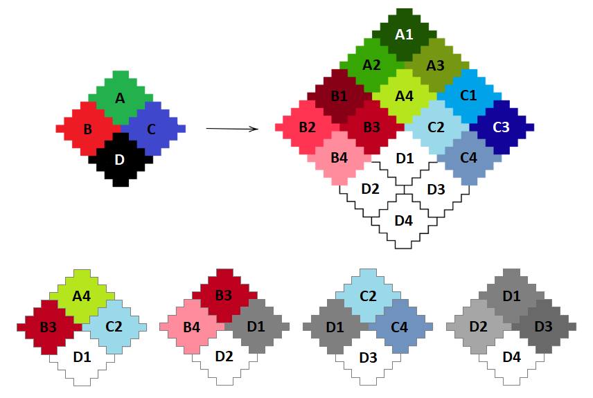
Figure 11: Upper - The results of applying the Scaffolding-Tile Generation technique on incomplete Tile D, with scaffolding Tiles A, B, and C. Lower - The Tiles referenced within the scaffolding variable of each resultant image Tile from D.

Once the image Tiles of incomplete Tile $T$ have had their value variables computed, the function performs the following steps for each image:

1. Check whether the tile value is unseen in the execution of the implementation so far. This is completed efficiently by leveraging the search capabilities of the tiles dictionary:

   • To search a dictionary, a key is provided, which the code will then complete a hashing function on. The result of the hashing function on the key provides a memory address that is unique to that specific key, allowing the value associated with that key to be retrieved.

   • The input_generator function utilises this process to check Tile uniqueness by using the image Tile’s computed value as the key to tiles. If data is returned from this computation then the Tile has already been found in an earlier computation, whereas if a null value is returned then this memory address has not been written to before, implying this must be a new unique Tile.

2. If the image value is unseen, instantiate the image into a Tile object, assigning the related Tiles to scaffolding as shown in the lower section of Figure 11. Then append the Tile into tiles and new_tiles.

After the Scaffolding-Tile Generation has executed, the incomplete Tile $T$ has each of its image Tiles assigned to it, and can now be considered complete. In cases where one of the image Tiles has been seen previously, a reference to the Tile object is retrieved from tiles for the purpose of assigning the image to $T$.

The input_generator function will have finished processing the image Tiles of every unique Tile once the new_tiles list is empty, at which point every unique Tile specific to this sequence, Tile length, and finite field has been found, along with its image under $\Phi$. The function then returns the tiles dictionary.

Part 2: Verifying the 2-Morphism

Once Part 1 has finished computation, the tiles dictionary contains a complete set of unique Tiles and their images under $\Phi$. However, it must now be verified that the two dimensional automatic sequence provided by the successful execution of the tile_computation is equal to the number wall.

Algorithm 2.1: Generating all possible 4-tuples

Before identifying any currently unrepresented 4-tuples in the data, the generate_four_tuples function needs to convert the information in the tiles dictionary into a different representation focused around 4-tuples. To achieve this, two new data structures are defined:

• tuples_by_index - a list of each currently known 4-tuple, where the existing 4-tuples are generated from the four image Tiles of each unique Tile in the tiles dictionary.

• tuples - a dictionary of every unique 4-tuple computed so far, where both the key and value of the entries are the 4-tuples themselves. This dictionary is immediately populated with the existing known 4-tuples from tuples_by_index. The sole purpose of this data structure is to allow the uniqueness of each newly generated 4-tuple to be verified efficiently.

Once these data structures have been instantiated, the generate_four_tuples function iterates through every 4-tuple in tuples_by_index and converts all of the images of each Tile in the 4-tuple into a singular grid. This essentially forms a 16-tuple (or image tuple), and mirrors the diagram shown in the upper row of Figure 11. However, for simplicity in the implementation, the diamond shape of the image tuple is rotated onto its side, allowing a square nested list to be used to represent the 2-dimensional space. Similarly, to save computation, this function does not handle the raw Tile values. Instead each tile is represented by its Tile id during each step of the computation.

From the image tuple, 5 new, potentially unseen 4-tuples are sampled. These are generated from the confluence points between Tile images from the original 4-tuple, i.e. where unrelated image 4-tuples meet. Using the top diagram in Figure 11 as an example, the following new 4-tuples would be sampled:

• Upper tuple - containing the Tiles B1, B3, A2, A4.

• Right tuple - containing the Tiles A3, A4, C1, C2.

• Left tuple - containing the Tiles B3, B4, D1, D2.

• Lower tuple - containing the Tiles D1, D3, C2, C4.

• Middle tuple - containing the Tiles A4, B3, C2, D1.

Each of these new 4-tuples is then checked for uniqueness, using the same hash map technique described in Algorithm 1.2. If any of the new 4-tuples are not currently contained in tuples (and are thus previously unseen), they are added to both tuples and tuples_by_index. Once every 4-tuple in tuples_by_index has been processed, all the unique 4-tuples that were previously unrepresented in the tiles data structure will have been identified. The generate_four_tuples function then returns the tuples_by_index list.

Algorithm 2.2: Verifying the 4-tuples

The final stage of the implementation is to verify that all of the identified 4-tuples conform to the Frame Constraints. The verify_four_tuples function takes the tuples_by_index list and tiles dictionary as inputs, and instantiates the following data structure to aid in the verification process:

• tiles_by_index - a pre-populated list of each Tile identified in Algorithm 1.2 (copied from tiles), where each item in the list is a reference to a Tile object, ordered by ascending Tile id. The list is used to assist in populating 4-tuples with Tile values, using the Tile ids already contained in each 4-tuple to retrieve the related Tiles.

The core of the function is completed by iterating through each 4-tuple in tuples_by_index, skipping the Zeroth Tile and First Tile (which cannot be generated using the Frame Constraints). For each 4-tuple that is processed, the function generates a square 2-dimensional list of junk data with a length twice as large as tile_length. This is generated to serve as a blank slate for inserting Tile values into, and is square to reduce the complexity of the list indexing required to construct each Tile’s value in the correct location. Following this, the value for the upper, left, and right Tile from the 4-tuple are inserted into the square - at which point the 4-tuple is ready to be verified.

To assess the correctness of the prepared 4-tuple, the verify_four_tuples function utilises the same Scaffolding-Tile Generation technique from Algorithm 1.2 - using the Frame Constraints with the three inserted Tiles to generate the missing, lower Tile. Using Figure 11 as an example, this would involve inputting Tiles A, B, and C as a scaffolding to generate Tile D in the top left portion of the diagram. This generated fourth Tile is then compared to the actual value of the fourth tile in the 4-tuple, which can be found using the Tile id stored in the lower portion of the 4-tuple. If the two Tiles do not have matching values, then the verification of that 4-tuple is considered to have failed.

If any of the 4-tuples fail their verification, then the entire function exits with a failure result. However, if every single 4-tuple is processed successfully by the verification function, then the entire set of Tiles and substitution rules should be considered accurate for the sequence, finite field, and tile length.

Samuel Garrett
samuel.garrett96@gmail.com Steven Robertson
School of Mathematics The University of Manchester Alan Turing Building Manchester, M13 9PL United Kingdom steven.robertson@manchester.ac.uk

References

- [ANL21] Faustin Adiceam, Erez Nesharim, and Fred Lunnon. On the t-adic littlewood conjecture. Duke Mathematical Journal, 170(10):2371–2419, July 2021.
- [APWW98] Jean-Paul Allouche, Jacques Peyrière, Zhi-Xiong Wen, and Zhi-Ying Wen. Hankel determinants of the thue-morse sequence. Annales de l’Institut Fourier, 48(1):1–27, 1998. doi:10.5802/aif.1609.
- [AS03] Jean-Paul Allouche and Jeffrey Shallit. Automatic Sequences: Theory, Applications, Generalizations. Cambridge University Press, 2003.
- [Bad21] D. Badziahin. On -adic littlewood conjecture for certain infinite products. Proc. Amer. Math. Soc., 149(11):4527–4540, 2021. doi:10.1090/proc/15475.
- [BBEK15] Dmitry Badziahin, Yann Bugeaud, Manfred Einsiedler, and Dmitry Kleinbock. On the complexity of a putative counterexample to the -adic littlewood conjecture. Compositio Mathematica, 151(9):1647–1662, 2015. doi:10.1112/S0010437X15007393.
- [BM08] Yann Bugeaud and Bernard Mathan. On a mixed littlewood conjecture in fields of power series. AIP Conference Proceedings, 976:19–30, 2008. doi:10.1063/1.2841906.
- [Bug09] Yann Bugeaud. Multiplicative diophantine approximation. Dynamical systems and Diophantine approximation, 19:105–125, 2009.
- [Bug14] Yann Bugeaud. Around the Littlewood conjecture in Diophantine approximation. Publications mathématiques de Besançon. Algèbre et théorie des nombres, pages 5–18, 2014. doi:10.5802/pmb.1.
- [CG95] John H. Conway and Richard K. Guy. The Book of Numbers. Copernicus New York, NY, 1995. doi:10.1007/978-1-4612-4072-3.
- [Cob72] Alan Cobham. Uniform tag sequences. Mathematical systems theory, 6:164–192, 1972. URL: https://api.semanticscholar.org/CorpusID:28356747.
- [EK07] Manfred Einsiedler and Dmitry Kleinbock. Measure rigidity and -adic littlewood-type problems. Compositio Mathematica, 143(3):689–702, 2007. doi:10.1112/S0010437X07002801.
- [EKL06] Manfred Einsiedler, Anatole Katok, and Elon Lindenstrauss. Invariant measures and the set of exceptions to littlewood’s conjecture. Annals of Mathematics, 164(2):513–560, 2006. URL: http://www.jstor.org/stable/20159999.
- [ELM17] Manfred Einsiedler, Elon Lindenstrauss, and Amir Mohammadi. Diagonal actions in positive characteristic. Duke Mathematical Journal, 169:117,175, 2017. doi:10.1215/00127094-2019-0038.
- [Hof18] Roswitha Hofer. Kronecker–halton sequences in fp((x-1)). Finite Fields and Their Applications, 50:154–177, 2018.
- [LEV22] Mordechay B. LEVIN. On a bounded remainder set for a digital kronecker sequence. Journal de Théorie des Nombres de Bordeaux, 34(1):163–187, 2022.
- [Lun01] William Lunnon. The number-wall algorithm: An lfsr cookbook. Journal of Integer Sequences, 4:2–3, 01 2001.
- [Lun09] Fred Lunnon. The pagoda sequence: a ramble through linear complexity, number walls, d0l sequences, finite state automata, and aperiodic tilings. Electronic Proceedings in Theoretical Computer Science, 1:130–148, 06 2009. doi:10.4204/eptcs.1.13.
- [Lun17] Fred Lunnon. Dragon wall tiling program and data, 2017. URL: https://github.com/FredLunnon/dragon_wall/.
- [MT04] Bernard Mathan and Olivier Teulié. Problèmes diophantiens simultanés. Monatshefte für Mathematik, 143:229–245, 11 2004. doi:10.1007/s00605-003-0199-y.
- [Nes] Erez Nesharim. t-adic littlewood in , number wall. CoCalc Collaborative Calculation in the Cloud. Last accessed 18/03/2024. URL: https://cocalc.com/share/public_paths/08de347bd272dd9a28a08531aecf5c6f3573f85e.
- [Que09] Martine Queffélec. An introduction to littlewood’s conjecture. Dynamical systems and Diophantine approximation, 19:127–150, 2009.
- [RG] Steven Robertson and Samuel Garrett. Number wall code. URL: https://github.com/Steven-Robertson2229/Counterexamples_to_the_p-t-_adic_Littlewood_Conjecture_Over_Small_Finite_Fields.git.
- [Rob23] Steven Robertson. Combinatorics on number walls and the -adic littlewood conjecture, 2023. arXiv:2307.00955.