JointRF: End-to-End Joint Optimization for Dynamic Neural Radiance Field Representation and Compression

Abstract

Neural Radiance Field (NeRF) excels in photo-realistically static scenes, inspiring numerous efforts to facilitate volumetric videos. However, rendering dynamic and long-sequence radiance fields remains challenging due to the significant data required to represent volumetric videos. In this paper, we propose a novel end-to-end joint optimization scheme of dynamic NeRF representation and compression, called JointRF, thus achieving significantly improved quality and compression efficiency against the previous methods. Specifically, JointRF employs a compact residual feature grid and a coefficient feature grid to represent the dynamic NeRF. This representation handles large motions without compromising quality while concurrently diminishing temporal redundancy. We also introduce a sequential feature compression subnetwork to further reduce spatial-temporal redundancy. Finally, the representation and compression subnetworks are end-to-end trained combined within the JointRF. Extensive experiments demonstrate that JointRF can achieve superior compression performance across various datasets.

Index Terms—  Volumetric Videos, Dynamic NeRF, Compression, End-to-end Joint Optimization.

1 Introduction

Photo-realistic volumetric video offers an immersive experience in virtual reality and telepresence. Dynamic Neural Radiance Field (NeRF)[1] has shown significant potential in representing photo-realistic volumetric video. However, there are still challenges in storing and transmitting volumetric video using NeRF, especially for sequences involving arbitrary motions and long durations. The difficulty lies in identifying an efficient representation and compression method for dynamic NeRF to deliver and store lengthy sequences.

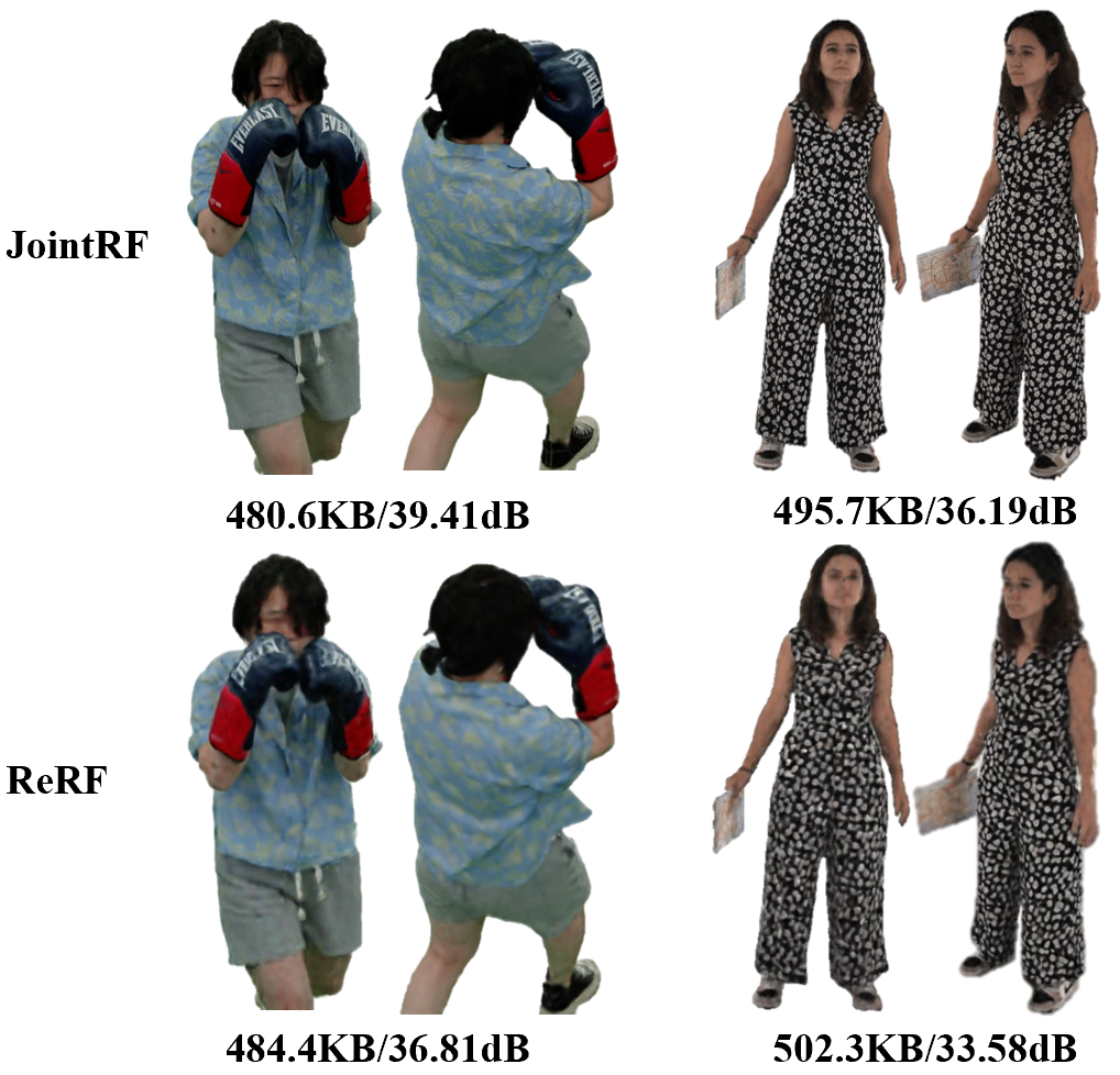
Fig. 1: The reconstructed results of our proposed JointRF compared to ReRF[2] on various datasets.

NeRF and its variants[1, 3, 4] have achieved significant success in synthesizing novel views, surpassing existing 3D reconstruction methods. The state-of-the-art visual quality has inspired numerous derivative research studies on dynamic scenes. Directly extending per-frame static NeRF methods to dynamic scenes is impractical, as they neglect the spatiotemporal continuity of scenes, resulting in an excess of network parameters. Some methods[5, 6, 7] attempt to recreate features in each frame by warping them back into canonical space. However, relying solely on the canonical space restricts the effectiveness of sequences with significant motion or topological changes.

Other approaches[8, 9, 10] extend the radiance field to 4D spatial-temporal domains, yet these methods face suboptimal rendering quality and encounter challenges related to large model storage, especially in streaming scenarios. Limited efforts have focused on compressing the dynamic radiance field for streaming, with ReRF[2] being a representative work. Although ReRF[2] has achieved some redundancy reduction in dynamic features through the traditional image encoding method, the traditional image encoder is unsuitable for high-dimensional feature domains. Additionally, ReRF[2] does not jointly optimize the representation and compression of the radiance field, leading to the loss of dynamic details and a decrease in compression efficiency.

In this paper, we present JointRF, a novel approach that jointly optimizes the representation and compression of dynamic NeRF, achieving better quality and higher compression efficiency (see Fig.1). Inspired by DiF [11], the radiance field is decomposed into a coefficient feature grid and a basis feature grid. JointRF explicitly models the residual feature grid between the long-reference basis and the non-long-reference basis. JointRF only utilizes a long-reference basis and a coefficient grid to represent the first keyframe. In contrast, for each subsequent frame, a compact residual grid along with a coefficient grid is used to compensate for errors and newly observed regions. A major advantage of this representation is the full utilization of feature relevance between adjacent frames.

Moreover, the feature grids of the representation are sequentially quantized and entropy encoded to further reduce redundancy. More importantly, we conduct end-to-end joint optimization for both the representation and compression processes, significantly enhancing the rate-distortion (RD) performance. Considering the non-differentiability of quantization and entropy coding in the compression process, we use simulated quantization and entropy model-based bitrate estimation to facilitate end-to-end training. Experimental results show that JointRF outperforms the state-of-the-art methods in terms of RD performance. To summarize, our contributions include:

• We propose a novel end-to-end learning scheme, called JointRF, that can jointly optimize both dynamic NeRF representation and compression. Our approach achieves superior RD performance and eliminates the need for intricate multi-stage training.

• We present an efficient and compact representation, representing the 4D radiance field into a series of residual feature grids to support streamable dynamic and long-sequence radiance field.

• We introduce an entropy-minimization compression method to guarantee the radiance field features with low entropy.

2 Related work

2.1 Dynamic Radiance Field Representation

Generating realistic synthesized views becomes more challenging in dynamic scenes, particularly due to the presence of moving objects. The canonical space methods[5, 6, 7] recover temporal features by warping the live-frame space back into the canonical space, which is fragile to large motions and topological changes. Another category of methods[8, 9, 10, 12, 13, 14, 15] extends the radiance field to 4D spatial-temporal domains, where they model the time-varying radiance field in a higher-dimensional feature space. ReRF[2] adopts the residual radiance field technique by leveraging compact motion grids and residual feature grids to exploit inter-frame feature similarity, achieving favorable outcomes in representing long sequences of dynamic scenes.

2.2 NeRF Compression

Recently, there has been limited attention to compressing static NeRF to reduce storage usage. VQRF[16] employs an entropy encoder to compress the static radiance field model, while ECRF[17] maps radiance field features to the frequency domain before applying entropy encoding. However, these methods remain confined to static scenes, and there has been relatively little exploration in compressing dynamic scenes. ReRF[2] is designed for modeling dynamic scenes and utilizes traditional image compression methods for further feature compression. However, due to the separate representation and compression processes in ReRF[2], it lacks end-to-end optimization. Moreover, traditional image encoders are unsuitable for compressing feature grids, resulting in suboptimal compression efficiency.

3 Method

In this section, we introduce the details about the proposed JointRF representation for long-sequence dynamic scenes (Sec.3.1), followed by an end-to-end joint optimization scheme for representation and compression (Sec.3.2).

3.1 JointRF Representation

Recall that NeRF[1] employs an implicit function to represent scenes. This function uses a large multi-layer perceptron (MLP) to map spatial coordinate $\mathbf{x}=(x,y,z)$ and view direction $\mathbf{d}$ to color $\mathbf{c}$ and density $\sigma$. By accumulating the colors $\mathbf{c}_{i}$ and densities $\sigma_{i}$ of all sampled points along a ray $\mathbf{r}$, we can derive the predicted color $\hat{\mathbf{c}}(\mathbf{r})$ for the corresponding pixel:

$$\hat{\mathbf{c}}(\mathbf{r})=\sum_{i}^{N}T_{i}(1-exp(-\sigma_{i}\delta_{i}))\mathbf{c}_{i},$$ (1)

where $T_{i}=exp(-\sum^{i-1}_{j=1}\sigma_{i}\delta_{i})$, and $\delta_{i}$ denotes the distance between adjacent samples.

To maintain high efficiency in training and rendering, we adopt an explicit representation similar to previous work [11]. The representation of a static scene is decomposed into the coefficient feature grid $\mathbf{C}$ and the basis feature grid $\mathbf{B}$ via basis expansion. The basis feature grid captures signal commonality, while the coefficient feature grid depicts spatial variations. The radiance field of a static scene can then be expressed as:

$$(\mathbf{c},\sigma)=\Phi(interp(\mathbf{x},\mathbf{C})\circ interp(\mathbf{x},\mathbf{B}),\mathbf{d}),$$ (2)

where $\Phi$ is a tiny MLP, and $interp(\cdot)$ represents the interpolation function on the grids. $\circ$ denotes a Hadamard product.

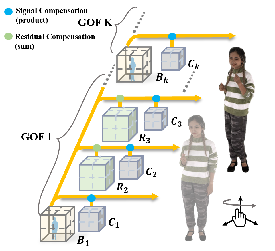
Fig. 2: Overview of JointRF representation. We divide the sequence into several GOFs. Each GOF starts with a keyframe, represented by a long-reference basis feature grid and a coefficient feature grid. Each subsequent frame in the GOF is then represented by a residual feature grid $\mathbf{R}_{t}$ in conjunction with a coefficient feature grid $\mathbf{C}_{t}$.

When extending the radiance field from a static scene to a dynamic one, a simplistic approach might involve employing individual per-frame feature grids $\{\mathbf{B}_{t},\mathbf{C}_{t}\}_{t=1}^{N}$ for the dynamic scene consisting of $N$ frames. However, this method fails to account for crucial temporal coherence. This not only leads to discontinuities in visual quality during significant motion but also results in excessive data volume due to the presence of substantial temporal redundancy, posing a particularly severe issue for long sequences in dynamic scenes.

To enhance temporal continuity while minimizing redundancy, we propose a highly compact representation method. The overview of our representation method is illustrated in Fig.2. We represent the long sequence of dynamic radiance field over time as multiple continuous groups of feature grids (GOF), which is a collection of successive grids. Each GOF $\mathbf{G}=\{\mathbf{f}_{t}\}_{t=1}^{N}$ begins with a keyframe $\mathbf{f}_{1}=\{\mathbf{B}_{1},\mathbf{C}_{1}\}$, which is a long reference feature grid. Due to the commonality captured by the basis in signal extraction and the short-term similarity of features, each remaining frame in the GOF is represented as a compact residual grid along with a coefficient grid ($\mathbf{f}_{t}=\{\mathbf{R}_{t},\mathbf{C}_{t}\}$, $1<t\leq N$). The residual feature grid $\mathbf{R}_{t}$ indicates the compensation for errors and newly observed regions between the keyframe’s basis grid and the current frame’s basis grid. $\mathbf{R}_{t}$ helps enhance the representation by incorporating residual information and reducing temporal redundancy. Once obtained $\mathbf{R}_{t}$, we can calculate the basis feature grid of the $t$-th frame by adding the residual compensation:$\mathbf{B}_{t}=\mathbf{B}_{1}+\mathbf{R}_{t}$, enabling the recovery of the current radiance field by applying the signal compensation according to Eq.(2).

Note that our JointRF representation enables efficient sequential feature modeling with several key advantages. Firstly, it leverages the simplicity of the residual data distribution, making it easier to compress and transmit compared to the complete data distribution. Secondly, our representation handles large motions without compromising quality. Additionally, since our method relies on only one keyframe during rendering, it enables simultaneous rendering of multiple non-keyframes, facilitating parallel computation. Furthermore, this representation supports frame-by-frame loading and rendering, reducing memory usage and favoring streaming.

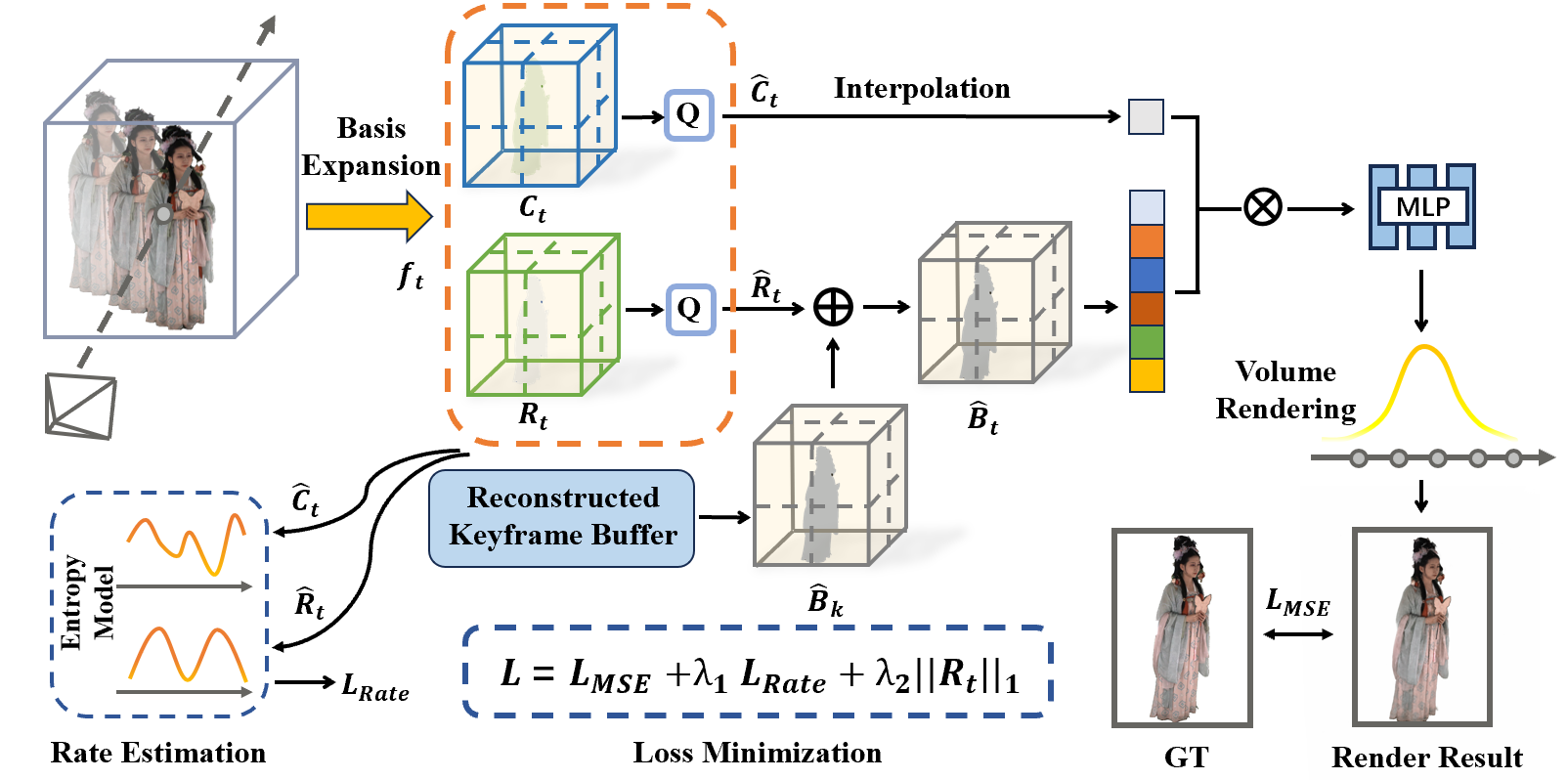
Fig. 3: Overview of our JointRF training. First, we apply simulated quantization to generate $\mathbf{\hat{C}}_{t}$ and $\mathbf{\hat{R}}_{t}$, and then estimate the rate of $\mathbf{\hat{C}}_{t}$ and $\mathbf{\hat{R}}_{t}$ as loss during the forward pass. Next, we load the long-reference basis feature grid $\mathbf{\hat{B}}_{k}$ from the reconstructed keyframe buffer and combine it with $\mathbf{\hat{C}}_{t}$ and $\mathbf{\hat{R}}_{t}$ to obtain the MSE loss. Finally, we sequentially train each frame and update the residual feature grid, coefficient feature grid, and the corresponding entropy model.

3.2 End-to-end Joint Optimization

Here, we introduce an end-to-end optimization approach that jointly optimizes the representation and compression of dynamic radiance field to further improve compression efficiency. The overall framework of our proposed approach is illustrated in Fig.3. We apply simulated quantization to the feature grid $\mathbf{f}_{t}$ and utilize an entropy model-based bitrate estimation to facilitate end-to-end training. The objective of JointRF is to ensure that the radiance field representation learned from modeling has low entropy while maintaining high reconstruction quality.

Simulated Quantization. The quantization operation can effectively reduce bitrate of the feature grids during the compression process, but it also results in a certain degree of information loss. Introducing quantization operation during training can effectively enhance the model’s robustness to the quantization loss. However, the rounding operation disrupts gradient propagation and makes it incompatible with end-to-end training. Since quantized value $\mathbf{Q}(x)\in[x-\frac{1}{2},x+\frac{1}{2}]$, we introduce uniform noise within the range of $[-\frac{1}{2},\frac{1}{2}]$ to simulate the quantization effect, as shown in Eq.(3), enabling gradient propagation.

$$\mathbf{Q}(x)=x+u,u\sim U(-\frac{1}{2},\frac{1}{2}).$$ (3)

Rate Estimation. We perform entropy encoding on the quantized feature grids to generate a highly compressed bitstream. If acquiring the bitrate during the training phase is possible, this metric could be integrated into the loss function to encourage a lower-entropy distribution of features, effectively imposing a bitrate constraint on the network updates. However, entropy encoding does not preserve gradients like the quantization process. To address this, we introduce an entropy model within the training phase to estimate the entropy of the grids, which is the lower bound of the bitrate after compression. The entropy model can approximate the probability mass function (PMF) of quantized $\hat{y}$ of a feature grid by computing the cumulative distribution function (CDF) of $\hat{y}$, as shown in Eq.(4).

$$P(\hat{y})=P_{CDF}(\hat{y}+\frac{1}{2})-P_{CDF}(\hat{y}-\frac{1}{2}).$$ (4)

To maintain precision, we refrain from presuming any preconceived data distribution for the 3D grids. Instead, we construct a novel distribution within the entropy model to closely match the actual data distribution. During training, the entropy model predicts the size of the compressed bitstream as part of the overall loss. The training process of JointRF can be seen in Fig.3.

On the encoding side of compression, we employ quantization followed by entropy encoding, specifically a rangecoder to compress the features and get the bitstream. On the decoding side, entropy decoding is performed to recover the features. The entire procedure unfolds as follows:

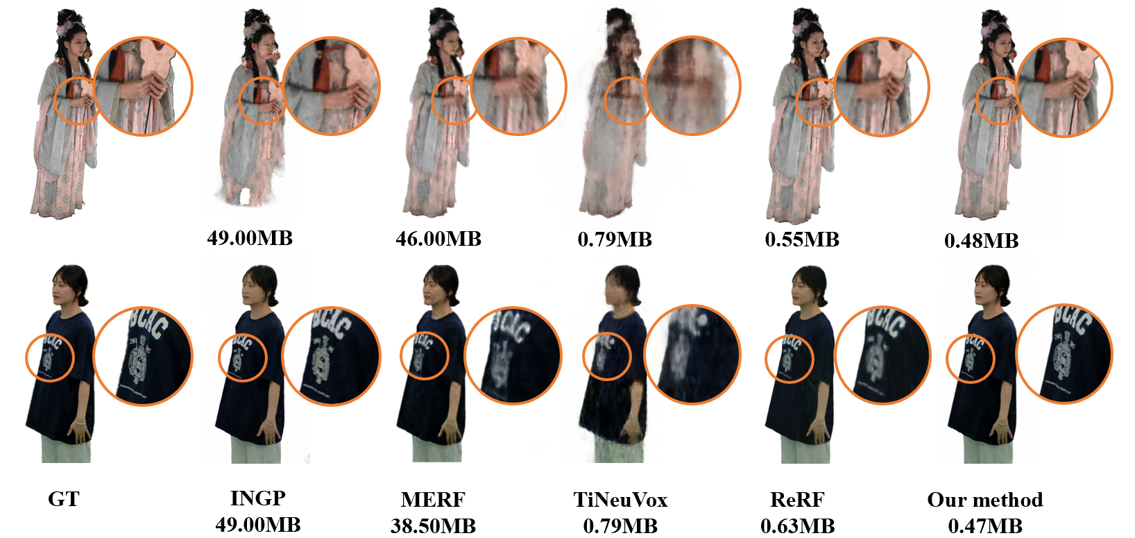
Fig. 4: Qualitative comparison against dynamic scene reconstruction methods and per-frame static reconstruction methods.

$$\hat{x}=\frac{\mathbf{D}(\mathbf{E}\left(\mathbf{Q}(q\cdot x)-\mathbf{Q}\left(q\cdot\min(x)\right)\right))+\mathbf{Q}(q\cdot\min(x))}{q},$$ (5)

where $\mathbf{E}$ is the entropy encoder, $\mathbf{D}$ is the entropy decoder and $\mathbf{Q}$ represents the quantization operation. To enable compression into int8 format, we convert the compressed data to non-negative values and subsequently revert it to its original range during decompression. The variable $q$ is the quantization parameter. During quantization, data is multiplied by $q$, effectively expanding the data range, which, in turn, subtly enhances quantization precision. By adjusting the parameter $q$, a trade-off can be made between reconstruction quality and model storage. A higher value of $q$ yields improved model reconstruction quality, but also increases the size of the compressed model.

Training Objective. The total loss function of the entire system can be written as below:

$$\mathcal{L}_{total} =\mathcal{L}_{mse}+\lambda_{1}\mathcal{L}_{rate}+\lambda_{2}||\mathbf{R}_{t}||_{1},$$ (6)

$$\mathcal{L}_{mse} =\sum||\mathbf{c}(\mathbf{r})-\hat{\mathbf{c}}(\mathbf{r})||^{2},$$ (7)

$$\mathcal{L}_{rate} =-\frac{1}{N}\sum_{\hat{y}\in\hat{\mathbf{R}}_{t}}{\log_{2}\left(P_{1}(\hat{y})\right)}-\frac{1}{M}\sum_{\hat{y}\in\hat{\mathbf{C}}_{t}}{\log_{2}\left(P_{2}(\hat{y})\right)},$$ (8)

where $\mathcal{L}_{mse}$ metrics the difference between the ground truth and the result rendered by JointRF. $\mathcal{L}_{rate}$ represents the estimated rate derived from $\hat{\mathbf{R}}_{t}$ and $\hat{\mathbf{C}}_{t}$. $||\mathbf{R}_{t}||_{1}$ is L1 regularization applied to $\mathbf{R}_{t}$ to ensure temporal continuity and minimize the magnitude of $\mathbf{R}_{t}$ . The parameter $\lambda_{1}$ is used to balance the rate and distortion, allowing for control over the model size and reconstruction quality. The parameter $\lambda_{2}$ measures the extent of our constraint on $\mathbf{R}_{t}$.

4 Experimental Results

4.1 Configurations

Datasets. In this section, we extensively assess JointRF through experiments conducted on five sequences: two from the ReRF[2] dataset and three from the DNA-Rendering[18] dataset. The ReRF dataset comprises 74 camera views, of which we designate 70 for training and the remaining 4 for testing. Images in this dataset have a resolution of $1920\times 1080$. The DNA-Rendering dataset, on the other hand, includes 48 views, with 46 used for training and 2 for testing. Images in this dataset have a resolution of $2048\times 2448$.

Setups. During the quantization phase, we typically evaluate four distinct $q$ values: 1, 2, 5, 10. For loss function, we initialize both $\lambda_{1}$ and $\lambda_{2}$ at 0.000001 and allow $\lambda_{1}$ decrementing progressively. For feature fitting, we employ seven distinct entropy models, each corresponding to the dimensions of the six different-resolution basis grids and the single coefficient grid. In our experimental setup, the length of each GOF is customarily fixed at 10.

4.2 Comparison

To the best of our knowledge, JointRF is a rare method for jointly training dynamic NeRF and their associated compression processes in a unified end-to-end manner. To validate the effectiveness of our approach, we compare with several state-of-the-art methods for dynamic scenes including INGP[3], MERF[4], TiNeuVox[14], ReRF[2] both qualitatively and quantitatively. In Fig.4, we present the visual results of two sequences. As illustrated, our method demonstrates discernible superiority in both the compactness of the model size and the precision of detail rendering not only on per-frame static reconstruction method INGP[3] and MERF[4] but also on dynamic scene reconstruction methods TiNeuVox[14] and ReRF[2].

Dataset	Method	Training View		Testing View		Size (MB) $\downarrow$
		PSNR $\uparrow$	SSIM $\uparrow$	PSNR $\uparrow$	SSIM $\uparrow$
ReRF	MERF[4]	32.99	0.981	27.33	0.964	38.5
	INGP[3]	36.48	0.989	28.57	0.966	49.0
	TiNeuVox[14]	30.19	0.962	22.39	0.950	0.81
	ReRF[2]	37.03	0.990	30.04	0.977	0.58
	Ours	38.68	0.992	33.23	0.980	0.47
DNA- Rendering	MERF[4]	33.24	0.975	27.52	0.958	46.0
	INGP[3]	34.13	0.979	24.22	0.960	49.0
	TiNeuVox[14]	30.28	0.953	22.15	0.945	0.80
	ReRF[2]	34.28	0.981	29.39	0.977	0.60
	Ours	35.17	0.982	31.83	0.978	0.48

Table 1: Quantitative comparison against dynamic scene reconstruction methods and per-frame static reconstruction methods. We calculate the average PSNR, SSIM, and storage for each frame across all training and testing views, separately.

We also conduct a quantitative comparison in terms of Peak Signal-to-Noise Ratio (PSNR), Structural Similarity Index (SSIM), and model storage as shown in Table 1. It can be seen that our method outperforms other methods and achieves the best reconstruction quality with the lowest model storage. INGP[3] requires a large amount of storage load when modeling 3D scenes, and cannot model unknown perspectives well. Although MERF[4] can reduce the storage load through baking operations, it still requires dozens of MB, and the reconstruction effect is not satisfactory. TiNeuVox[14], on the other hand, is capable of representing sequences of arbitrary length within a consistent memory footprint. However, it suffers from severe blurring effects as the frame count increases. Compared to ReRF[2], our method performs better in terms of PSNR, SSIM, and model storage as well.

Table 2 shows a comparison of RD performance between our JointRF and ReRF[2]. Notably, our JointRF achieves a better RD performance compared to ReRF. On the ReRF dataset, we observe average BDBR reductions of 51.28% and 69.66% for training and testing views, respectively. Similarly, on the DNA-Rendering dataset, the average BDBR saving is 35.06% and 36.38% for training and testing views, respectively. The superior performance of our method can be attributed to the fact that ReRF[2] employs a traditional encoder, which is unsuitable for feature grid compression. In contrast, JointRF conducts an end-to-end joint optimization of representation and compression, leading to enhanced RD performance.

Dataset	Training View		Testing View
	BD-PSNR (dB) $\uparrow$	BDBR (%) $\downarrow$	BD-PSNR (dB) $\uparrow$	BDBR (%) $\downarrow$
ReRF	3.12	-51.28	5.18	-69.66
DNA-Rendering	1.88	-35.06	1.96	-36.38

Table 2: The BDBR results of our JointRF when compared with ReRF[2] on different datasets.

4.3 Ablation Studies

We conduct three ablation studies on both training and testing views on ReRF and DNA-Rendering datasets to validate the effectiveness of each component in our method by removing each of them individually. We mainly focus on the compression module, end-to-end joint optimization, and dynamic residual representation.

In the first ablation study, we removed the compression step while preserving the residual-based dynamic modeling. In the second experiment, we did not jointly optimize dynamic modeling and compression during training and performed compression after training completion. Finally, we individually modeled dynamic scenes frame by frame and conducted joint optimization without introducing residual-based representation.

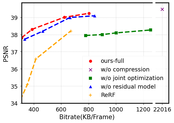
(a) ReRF (Train)

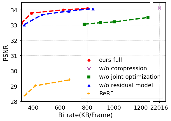
(b) ReRF (Test)

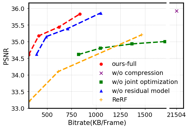
(c) DNA-Rendering (Train)

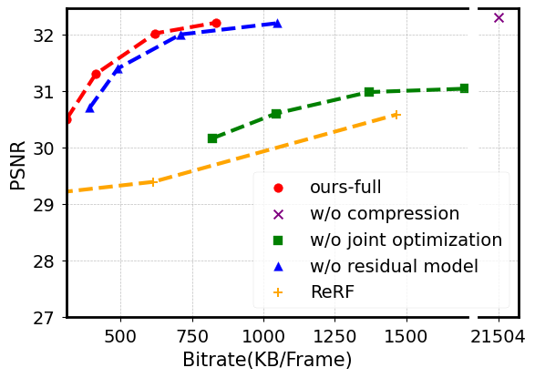
(d) DNA-Rendering (Test)

Fig. 5: Rate-distortion curves in both the ReRF and DNA-Rendering datasets. Rate-distortion curves not only illustrate the efficiency of various components within our JointRF but also demonstrate its superiority over ReRF[2].

The results of the ablation studies can be seen in Fig.5. It shows that our compression method significantly reduces model storage by approximately 40 times while maintaining comparable reconstruction quality. What’s more, joint optimization can not only reduce the model size but also slightly improve PSNR because the features obtained through joint optimization are easier to compress and robust to quantization errors. Lastly, dynamic residual representation can effectively achieve better RD performance. The results of the ablation studies demonstrate the integral importance of our dynamic residual representation, compression module, and joint optimization strategy.

5 Conclusion

In this paper, we propose JointRF, a novel approach that jointly optimizes the representation and compression of dynamic NeRF. We first introduce a highly compact modeling method for representing dynamic and long-sequence NeRF. To further reduce the spatial-temporal redundancy, we devise a compression method that is concurrently optimized with the representation of dynamic NeRF, enabling end-to-end training. Instead of predetermining feature distributions, our approach models data distributions during training to enable precise bitrate estimations and quantitative differentiable approximations. Experimental results show that JointRF outperforms the state-of-the-art methods in terms of RD performance across various datasets. With its unique representation and compression capabilities for long-sequence dynamic scenes, we believe our approach lays the foundation for various potential applications in volumetric videos.

References

- [1] Ben Mildenhall, Pratul P Srinivasan, Matthew Tancik, Jonathan T Barron, Ravi Ramamoorthi, and Ren Ng, “Nerf: Representing scenes as neural radiance fields for view synthesis,” Communications of the ACM, vol. 65, no. 1, pp. 99–106, 2021.
- [2] Liao Wang, Qiang Hu, Qihan He, Ziyu Wang, Jingyi Yu, Tinne Tuytelaars, Lan Xu, and Minye Wu, “Neural residual radiance fields for streamably free-viewpoint videos,” in Proceedings of the IEEE/CVF Conference on Computer Vision and Pattern Recognition (CVPR), June 2023, pp. 76–87.
- [3] Thomas Müller, Alex Evans, Christoph Schied, and Alexander Keller, “Instant neural graphics primitives with a multiresolution hash encoding,” ACM Trans. Graph., vol. 41, no. 4, pp. 102:1–102:15, July 2022.
- [4] Christian Reiser, Rick Szeliski, Dor Verbin, Pratul Srinivasan, Ben Mildenhall, Andreas Geiger, Jon Barron, and Peter Hedman, “Merf: Memory-efficient radiance fields for real-time view synthesis in unbounded scenes,” ACM Transactions on Graphics (TOG), vol. 42, no. 4, pp. 1–12, 2023.
- [5] Keunhong Park, Utkarsh Sinha, Jonathan T. Barron, Sofien Bouaziz, Dan B Goldman, Steven M. Seitz, and Ricardo Martin-Brualla, “Nerfies: Deformable neural radiance fields,” in Proceedings of the IEEE/CVF International Conference on Computer Vision (ICCV), October 2021, pp. 5865–5874.
- [6] Albert Pumarola, Enric Corona, Gerard Pons-Moll, and Francesc Moreno-Noguer, “D-NeRF: Neural Radiance Fields for Dynamic Scenes,” in Proceedings of the IEEE/CVF Conference on Computer Vision and Pattern Recognition, 2020.
- [7] Yilun Du, Yinan Zhang, Hong-Xing Yu, Joshua B. Tenenbaum, and Jiajun Wu, “Neural radiance flow for 4d view synthesis and video processing,” in Proceedings of the IEEE/CVF International Conference on Computer Vision, 2021.
- [8] Mustafa Işık, Martin Rünz, Markos Georgopoulos, Taras Khakhulin, Jonathan Starck, Lourdes Agapito, and Matthias Nießner, “Humanrf: High-fidelity neural radiance fields for humans in motion,” ACM Transactions on Graphics (TOG), vol. 42, no. 4, 2023.
- [9] Jiemin Fang, Taoran Yi, Xinggang Wang, Lingxi Xie, Xiaopeng Zhang, Wenyu Liu, Matthias Nießner, and Qi Tian, “Fast dynamic radiance fields with time-aware neural voxels,” arXiv preprint arXiv:2205.15285, 2022.
- [10] Sara Fridovich-Keil, Giacomo Meanti, Frederik Rahbæk Warburg, Benjamin Recht, and Angjoo Kanazawa, “K-planes: Explicit radiance fields in space, time, and appearance,” in Proceedings of the IEEE/CVF Conference on Computer Vision and Pattern Recognition, 2023, pp. 12479–12488.
- [11] Anpei Chen, Zexiang Xu, Xinyue Wei, Siyu Tang, Hao Su, and Andreas Geiger, “Factor fields: A unified framework for neural fields and beyond,” arXiv preprint arXiv:2302.01226, 2023.
- [12] Ruizhi Shao, Zerong Zheng, Hanzhang Tu, Boning Liu, Hongwen Zhang, and Yebin Liu, “Tensor4d: Efficient neural 4d decomposition for high-fidelity dynamic reconstruction and rendering,” in Proceedings of the IEEE/CVF Conference on Computer Vision and Pattern Recognition, 2023, pp. 16632–16642.
- [13] Saskia Rabich, Patrick Stotko, and Reinhard Klein, “Fpo++: Efficient encoding and rendering of dynamic neural radiance fields by analyzing and enhancing fourier plenoctrees,” arXiv preprint arXiv:2310.20710, 2023.
- [14] Jiemin Fang, Taoran Yi, Xinggang Wang, Lingxi Xie, Xiaopeng Zhang, Wenyu Liu, Matthias Nießner, and Qi Tian, “Fast dynamic radiance fields with time-aware neural voxels,” in SIGGRAPH Asia 2022 Conference Papers. Nov. 2022, SA ’22, ACM.
- [15] Lingzhi Li, Zhen Shen, Zhongshu Wang, Li Shen, and Ping Tan, “Streaming radiance fields for 3d video synthesis,” Advances in Neural Information Processing Systems, vol. 35, pp. 13485–13498, 2022.
- [16] Lingzhi Li, Zhen Shen, Zhongshu Wang, Li Shen, and Liefeng Bo, “Compressing volumetric radiance fields to 1 mb,” in Proceedings of the IEEE/CVF Conference on Computer Vision and Pattern Recognition, 2023, pp. 4222–4231.
- [17] Soonbin Lee, Fangwen Shu, Yago Sanchez, Thomas Schierl, and Cornelius Hellge, “Ecrf: Entropy-constrained neural radiance fields compression with frequency domain optimization,” arXiv preprint arXiv:2311.14208, 2023.
- [18] Wei Cheng, Ruixiang Chen, Siming Fan, Wanqi Yin, Keyu Chen, Zhongang Cai, Jingbo Wang, Yang Gao, Zhengming Yu, Zhengyu Lin, et al., “Dna-rendering: A diverse neural actor repository for high-fidelity human-centric rendering,” in Proceedings of the IEEE/CVF International Conference on Computer Vision, 2023, pp. 19982–19993.