CoMERA: Computing- and Memory-Efficient Training via Rank-Adaptive Tensor Optimization

Abstract

Training large AI models such as deep learning recommendation systems and foundation language (or multi-modal) models costs massive GPUs and computing time. The high training cost has become only affordable to big tech companies, meanwhile also causing increasing concerns about the environmental impact. This paper presents CoMERA, a Computing- and Memory-Efficient training method via Rank-Adaptive tensor optimization. CoMERA achieves end-to-end rank-adaptive tensor-compressed training via a multi-objective optimization formulation, and improves the training to provide both a high compression ratio and excellent accuracy in the training process. Our optimized numerical computation (e.g., optimized tensorized embedding and tensor-network contractions) and GPU implementation eliminate part of the run-time overhead in the tensorized training on GPU. This leads to, for the first time, $2-3\times$ speedup per training epoch compared with standard training. CoMERA also outperforms the recent GaLore in terms of both memory and computing efficiency. Specifically, CoMERA is $2\times$ faster per training epoch and $9\times$ more memory-efficient than GaLore on a tested six-encoder transformer with single-batch training. With further HPC optimization, CoMERA may significantly reduce the training cost of large language models.

1 Introduction

Deep neural networks have gained success in solving numerous engineering problems. These approaches usually use a huge number of variables to parametrize a network, and require massive hardware resources to train the model. For instance, the Deep Learning Recommendation Model (DLRM) released by Meta (which is smaller than the practical product) [28] has 4.2 billion parameters; GPT-3 [4] has 175 billion parameters. OpenAI shows that the computing power required for key AI tasks has doubled every 3.4 months [1] since 2012. Training a large language model like ChatGPT and LLaMA from scratch often takes several weeks or months on thousands of GPUs [3, 2].

Large AI models often have much redundancy. Therefore, numerous methods have been developed to reduce the cost of AI inference [5, 21, 7, 10, 13, 27, 26, 14]). However, training large AI models (especially from scratch) remains an extremely challenging task. Low-precision training [16, 23, 9, 32] has been popular in on-device setting, but its memory reduction is quite limited. Furthermore, it is hard to utilize ultra low-precision training on GPU since current GPUs only support limited precision formats for truly quantized training. Chen [6] employed the idea of robust matrix factorization to reduce the training cost. Similar low-rank matrix approximation techniques have been applied to train large AI models including large language models [37, 17]. Among them, GaLore [37] can train the 7B LLaMA model on a RTX 4090 GPU using a single-batch and layer-wise setting. However, this setting can lead to extremely long training time, which is infeasible in practical settings.

Compared with matrix compression, low-rank tensor compression has achieved much higher compression ratios on various neural networks [29, 25, 36, 33, 18, 21]. This idea has been studied in fixed-rank training  [29, 5, 20], zeroth-order training [38] and parameter-efficient fine tuning [35]. The recent work [11, 12] provides a rank-adaptive tensor-compressed training from a Bayesian perspective. However, to achieve a reduction in both memory and training time (especially on transformers), two open problems need to be addressed. Firstly, a more robust rank-adaptive tensor-compressed training model is desired, since the method in [11, 12] replies on a heuristic fixed-rank warm-up training. Secondly, while modern GPUs are well-optimized for large-size matrix computations, they are unfriendly for low-rank tensor-compressed training. Specifically, most operations in tensor-compressed training are small-size tensor contractions, which can cause significant runtime overhead on GPUs even though the theoretical computing FLOPS is very low. As a result, as far as we know no papers have reported real training speedup on GPU. This issue was also observed in [15].

Paper Contributions.

In this work, we propose CoMERA, a tensor-compressed training method that can achieve, for the first time, simultaneous reduction of both memory and runtime on GPU. Our specific contributions are summarized as follows.

• Multi-Objective Optimization for Rank-Adaptive Tensor-Compressed Training. We propose a multi-objective optimization formulation to balance the compression ratio and model accuracy and to customize the model for a specific resource requirement. One by-product of this method is the partial capability of automatic architecture search: some layers are identified as unnecessary and can be completely removed by rank-adaptive training.

• Performance Optimization of Tensor-Compressed Training. While tensor-compressed training greatly reduces the memory cost and computing FLOPS, it often slows down the practical training on GPU. We propose three approaches to achieve real training speedup: ① optimizing the lookup process of tensorized embedding tables, ② optimizing the tensor-network contractions in both forward and backward propagation, ③ eliminating the GPU backend overhead via CUDA Graph.

• Experimental Results. We evaluate our method on the end-to-end training of a transformer with six encoders and the deep learning recommendation system model (DLRM). On these two benchmarks, our method achieves $80\times$ and $99\times$ compression ratios respectively, while maintaining the testing accuracy of standard uncompressed training. CoMERA also achieves $2-3\times$ speedup per training epoch compared with standard training methods on the transformer model.

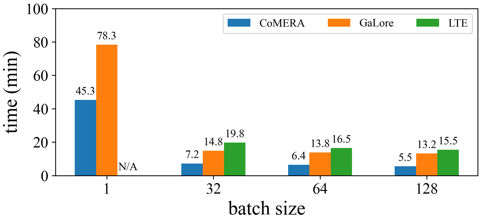
(a) Training time per epoch.

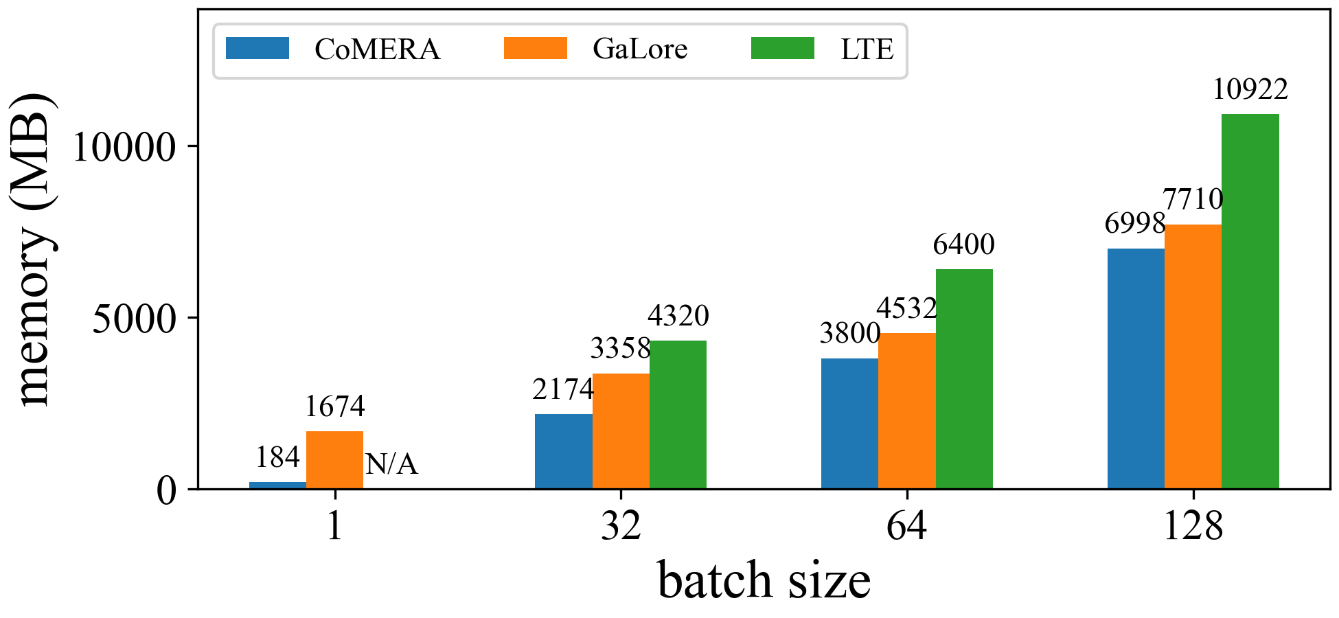
(b) Peak memory consumption.

Figure 1: Training time and total memory cost of CoMERA, GaLore [37] and LTE [17] on a six-encoder transformer with varying batch sizes. The experiment is done on Nvidia RTX 3090 GPU.

Figure 1 compares our CoMERA with GaLore [37] and the recent LoRA-based training method LTE [17] on the six-encoder transformer. When data and back-end memory cost are considered, CoMERA’s memory consumption is $9\times$ less than GaLore in the single-batch training as adopted in [37], and it uses the least memory under all batch sizes. Our method is $2-3\times$ faster than GaLore and LTE in each training epoch, although CoMERA has not yet been fully optimized on GPU.

While this work focuses on reducing the memory and computing cost of training, it can also reduce the communication cost by orders of magnitude: only low-rank tensorized model parameters and gradients need to be communicated in a distributed setting. The CoMERA framework can also be implemented on resource-constraint edge devices to achieve energy-efficient on-device learning.

2 Background

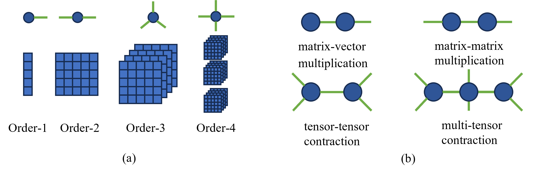
Figure 2: (a) Tensors. (b) Tensor contractions.

The tensor [22, 24] $\mathbfcal{A}\in\mathbb{R}^{n_{1}\times n_{2}\times\cdots\times n_{d}}$ is indexed as $\mathbfcal{A}=(a_{i_{1}\cdots i_{d}})_{1\leq i_{j}\leq n_{j}}$ and is said to have order $d$ and dimension $n_{1},\ldots,n_{d}$. The Frobenius norm of tensor $\mathbfcal{A}$ is defined as $\|\mathbfcal{A}\|:=\sqrt{\sum_{i_{1},\ldots,i_{d}}^{n_{1},\ldots,n_{d}}a_{i_{1}\cdots i_{d}}^{2}}$. In tensor networks, the order-$d$ tensor $\mathbfcal{A}$ is represented as a node with $d$ edges. Some tensor network representations are illustrated in Fig. 2 (a).

Tensor Contraction.

Let $\mathbfcal{A}\in\mathbb{R}^{n_{1}\times n_{2}\times\cdots\times n_{d}}$ and $\mathbfcal{B}\in\mathbb{R}^{l_{1}\times l_{2}\times\cdots\times l_{m}}$ be two tensors with $n_{s}=l_{t}$. The tensor contraction product $\mathbfcal{C}=\mathbfcal{A}\times_{s,t}\mathbfcal{B}$ has dimension $\Pi_{i\neq s}n_{i}\times\Pi_{j\neq t}l_{j}$ and the entries are

$$c_{(i_{p})_{p\neq s},(j_{p})_{p\neq t}}=\sum_{i_{s}=j_{t}=1}^{n_{s}}a_{i_{1}\cdots i_{s}\cdots i_{m}}b_{j_{1}\cdots j_{t}\cdots j_{k}}.$$ (1)

This definition can be naturally generalized to multiple pairs. Figure 2(b) illustrates some tensor contractions. For general operations among multiple tensors, we use PyTorch einsum in the following

$$\mathbfcal{B}=\mbox{\bf einsum}(S_{1},\ldots,S_{m}\Rightarrow T,[\mathbfcal{A}_{1},\ldots,\mathbfcal{A}_{m}]),$$ (2)

where each $S_{i}$ is a string of characters that specifies the dimension of $\mathbfcal{A}_{i}$. The output tensor $\mathbfcal{B}$ is obtained by summing over all other dimensions that are not in $T$. In the following, we show a few commonly used einsum operations. The Tensor-Train decomposition as in (3) is

$$\mathbfcal{A}=\mbox{\bf einsum}(n_{1}r_{1},\ldots,r_{d-1}n_{d}\Rightarrow n_{1}n_{2}\cdots n_{d},[\mathbfcal{G}_{1},\mathbfcal{G}_{2}\ldots,\mathbfcal{G}_{d}]).$$

For the batched matrices $\mathbfcal{A}\in\mathbb{R}^{b\times m\times k},\mathbfcal{B}\in\mathbb{R}^{b\times k\times n}$, the batched matrix multiplication is

$$\mathbfcal{C}=\mathbfcal{A}\mathbfcal{B}=\mbox{\bf einsum}(bmk,bkn\Rightarrow bmn,[\mathbfcal{A},\mathbfcal{B}]),\;\;\text{where}\;\mathbfcal{C}[i,:,:]=\mathbfcal{A}[i,:,:]\mathbfcal{B}[i,:,:].$$

Tensor Decomposition.

In this paper, we will mainly use tensor-train (TT) [31] and tensor-train matrix (TTM) [30] decomposition for compressed neural network training. TT [31] represents the tensor $\mathbfcal{A}\in\mathbb{R}^{n_{1}\times n_{2}\times\cdots\times n_{d}}$ as a set of small-size cores $\mathbfcal{G}_{1},\ldots,\mathbfcal{G}_{d}$ such that $\mathbfcal{G}_{i}\in\mathbb{R}^{r_{i-1}\times n_{i}\times r_{i}}$ and

$$\mathbfcal{A}=\mathbfcal{G}_{1}\times_{3,1}\mathbfcal{G}_{2}\times_{3,1}\cdots\times_{3,1}\mathbfcal{G}_{d}.$$ (3)

The tuple $(r_{0},r_{1},\ldots,r_{d})$ is the TT rank of the TT decomposition (3) and must satisfy $r_{0}=r_{d}=1$. TTM considers an order-$2d$ tensor $\mathbfcal{B}$ of dimension $m_{1}\times n_{2}\times\cdots\times m_{d}\times n_{d}$, and represents $\mathbfcal{B}$ as

$$\mathbfcal{B}=\mathbfcal{F}_{1}\times_{4,1}\mathbfcal{F}_{2}\times_{4,1}\cdots\times_{4,1}\mathbfcal{F}_{d},$$ (4)

where $\mathbfcal{F}_{i}\in\mathbb{R}^{r_{i-1}\times m_{i}\times n_{i}\times r_{i}}$ for $i=1,\ldots,d$ and $r_{0}=r_{d}=1$. Figure 3 shows the tensor-network representations of TT and TTM decomposition.

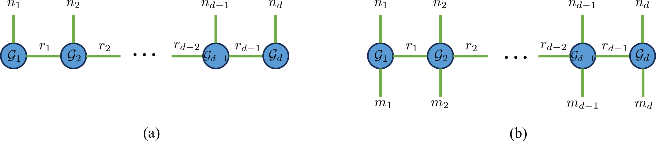
Figure 3: Tensor networks for (a) tensor-train and (b) tensor-train-matrix decompositions.

In tensor-compressed neural networks, large weight matrices are reshaped to high-order tensors and compressed into small tensor cores in TT or TTM format. The weights of linear layers are often compressed into the TT format due to its efficiency in tensor-vector multiplications. The TTM format is more suitable for embedding tables whose dimension is highly unbalanced.

3 The CoMERA Training Framework

The size of the tensor-compressed neural networks can be adjusted by modifying the tensor ranks. However, it also brings in an important problem: how can we determine the tensor ranks automatically for a given resource limit? We propose a multi-objective optimization to address this issue.

3.1 Multi-Objective Training Model

A Modified TT Representation.

We consider the tensor-compressed training for a generic neural network. Suppose that the neural network is parameterized as $f(\mathbf{x}|\{\mathbfcal{G}^{i}_{1},\ldots,\mathbfcal{G}^{i}_{d_{i}}\}_{i=1}^{P})$, where $\{\mathbfcal{G}^{i}_{j}\in\mathbb{R}^{r^{i}_{j-1}\times n^{i}_{j}\times r^{i}_{j}}\}_{j=1}^{d_{i}}$ compress the original weight $\mathbf{W}_{i}$. Let $\{\mathbf{x}_{k},y_{k}\}_{k=1}^{N}$ be training data and $\mathcal{L}$ be the loss function. The training is to minimize the following objective function

$$\min_{\{\mathbfcal{G}^{i}_{1},\ldots,\mathbfcal{G}^{i}_{d_{i}}\}_{i=1}^{P}}L:=\sum_{k=1}^{N}\mathcal{L}(y_{k},f(\mathbf{x}_{k}|\{\mathbfcal{G}^{i}_{1},\ldots,\mathbfcal{G}^{i}_{d_{i}}\}_{i=1}^{P})).$$ (5)

We modify the TT compression and control the ranks of $\mathbfcal{G}^{i}_{1},\ldots,\mathbfcal{G}^{i}_{d_{i}}$ by a set of diagonal matrices $\{\mathbf{D}^{i}_{j}\in\mathbb{R}^{r^{i}_{j}\times r^{i}_{j}}\}_{j=1}^{d-1}$. Specifically, let $\mathbfcal{W}_{i}$ be the reshape of $\mathbf{W}_{i}$, and the compression of $\mathbf{W}_{i}$ is

$$\mathbfcal{W}_{i}=\mathbfcal{G}^{i}_{1}\times_{3,1}\mathbf{D}^{i}_{1}\times_{2,1}\mathbfcal{G}^{i}_{2}\times_{3,1}\cdots\times_{3,1}\mathbf{D}^{i}_{d_{i}-1}\times_{2,1}\mathbfcal{G}^{i}_{d_{i}}.$$ (6)

Now the tensor cores for $\mathbfcal{W}_{i}$ have $S_{i}=n_{1}^{i}\|\mathbf{D}_{1}^{i}\|_{0}+n_{d_{i}}^{i}\|\mathbf{D}_{d_{i}-1}^{i}\|_{0}+\sum_{j=2}^{d_{i}-1}n^{i}_{j}\|\mathbf{D}_{j-1}^{i}\|_{0}\|\mathbf{D}_{j}^{i}\|_{0}$ variables. For simplicity, we denote $\mathbfcal{G}:=\{\mathbfcal{G}^{i}_{1},\ldots,\mathbfcal{G}^{i}_{d_{i}}\}_{i=1}^{P}$ and $\mathbf{D}:=\{\mathbf{D}_{1}^{i},\ldots,\mathbf{D}_{d_{i}-1}^{i}\}_{i=1}^{P}$.

Multi-Objective Optimization.

We intend to minimize both the loss and compressed network size, which can be formulated as a multi-objective optimization $\min_{\mathbfcal{G},\mathbf{D}}\left\{L(\mathbfcal{G},\mathbf{D}),S(\mathbf{D})\right\},$ where $S(\mathbf{D}):=\sum_{i=1}^{P}S_{i}(\mathbf{D})$. In most cases, we cannot find a point that minimizes the loss and model size simultaneously. Therefore, we look for a Pareto point $(\mathbfcal{G}^{*},\mathbf{D}^{*})$, meaning that there exist no $\mathbfcal{G}$ and $\mathbf{D}$ such that $L(\mathbfcal{G},\mathbf{D})\leq L(\mathbfcal{G}^{*},\mathbf{D}^{*})$, $S(\mathbf{D})\leq S(\mathbf{D}^{*})$, and at least one of inequalities is strict.

3.2 Training Methods

We convert a mutli-objective optimization to a single-objective one via scalarization. We use different scalarization methods at the early and late stage of training. The late stage is optional, and it can further compress the model to enable efficient deployment on resource-constraint platforms.

Early Stage.

At the early stage of CoMERA, aggressively pruning ranks dramatically hurts the convergence. Hence, we start the training with the following linear scalarization formulation [8]

$$\min_{\mathbfcal{G},\mathbf{D}}\,\,L(\mathbfcal{G},\mathbf{D})+\gamma{S}(\mathbf{D}).$$ (7)

It is still hard to solve (7) since $S(\mathbf{D})$ uses $\|\cdot\|_{0}$ which is nonsmooth. Therefore, we replace $\|\cdot\|_{0}$ by the $\ell_{1}$ norm $\|\cdot\|_{1}$ and get the convex relaxation

$$\hat{S}(\mathbf{D}):=\sum_{i=1}^{P}\left(\sum_{i=1}^{P}n_{1}^{i}\|\mathbf{D}_{1}^{i}\|_{1}+n_{d_{i}}^{i}\|\mathbf{D}_{d_{i}-1}^{i}\|_{1}+\sum_{j=2}^{d_{i}-1}n^{i}_{j}\|\mathbf{D}_{j-1}^{i}\|_{1}\|\mathbf{D}_{j}^{i}\|_{1}\right).$$ (8)

We note that $\hat{S}(\mathbf{D})$ can be arbitrarily close to $0$ while keeping $L(\mathbfcal{G},\mathbf{D})$ unchangeable, since the corresponding slices of TT factors can be scaled accordingly. Therefore, a direct relaxation of the scalarization (11) does not have a minimizer. To address this issue, we add an $\ell_{2}$ regularization $\|\mathbfcal{G}\|^{2}:=\sum_{i=1}^{P}\sum_{j=1}^{d_{i}}\|\mathbfcal{G}^{i}_{j}\|^{2}$ to the relaxation and get the formulation

$$\min_{\mathbfcal{G},\mathbf{D}}\,\,L(\mathbfcal{G},\mathbf{D})+\gamma\hat{S}(\mathbf{D})+\beta\|\mathbfcal{G}\|^{2}.$$ (9)

The optimizer of Problem (9) is a Pareto point for a constrained problem, shown in the following.

Proposition 3.1.

For all $\gamma>0,\beta>0$, there exists some constant $C>0$ such that the solution to the problem (9) is a Pareto point of the following multi-objective optimization problem

$$\min_{\mathbfcal{G},\mathbf{D}} (L(\mathbfcal{G},\mathbf{D}),\hat{S}(\mathbf{D})) \text{subject to}\,\|\mathbfcal{G}\|^{2}\leq C.$$ (10)

Proof.

See Appendix A.1 for the complete proof. ∎

Late Stage (Optional).

In the late stage of CoMERA, we may continue training the model towards a preferred loss $L_{0}$ and a preferred model size $S_{0}$ for deployment requirements. This can be achieved by using an achievement scalarization [8] that leads to a Pareto point close to $(L_{0},S_{0})$:

$$\min_{\mathbfcal{G},\mathbf{D}}\,\,\max\left\{w_{1}(L(\mathbfcal{G},\mathbf{D})-L_{0}),w_{2}(S(\mathbf{D})-S_{0})\right\}+\rho(L(\mathbfcal{G},\mathbf{D})+S(\mathbf{D})).$$ (11)

Here $w_{1},w_{2}>0$ scale the objectives into proper ranges, and $\rho>0$ is a small constant. After relaxing $S(\mathbf{D})$ to $\hat{S}(\mathbf{D})$ and adding the regularization term, we get the following problem

$$\min_{\mathbfcal{G},\mathbf{D}}\,\,\max\left\{w_{1}(L(\mathbfcal{G},\mathbf{D})-L_{0}),w_{2}({S}(\mathbf{D})-S_{0})\right\}+\rho(L(\mathbfcal{G},\mathbf{D})+\hat{S}(\mathbf{D}))+\beta\|\mathbfcal{G}\|^{2},$$ (12)

where $\beta>0$ is a positive constant. Note that the ${S}(\mathbf{D})$ inside $\max$ is not relaxed now for accurate comparisons. When $w_{1}(L(\mathbfcal{G},\mathbf{D})-L_{0})\geq w_{2}({S}(\mathbf{D})-S_{0})$, we consider the following problem

$$\min_{\mathbfcal{G},\mathbf{D}}\,\,w_{1}(L(\mathbfcal{G},\mathbf{D})-L_{0})+\rho(L(\mathbfcal{G},\mathbf{D})+\hat{S}(\mathbf{D}))+\beta\|\mathbfcal{G}\|^{2}.$$ (13)

We run a step of a gradient-based algorithm on this problem. When $w_{1}(L(\mathbfcal{G},\mathbf{D})-L_{0})<w_{2}({S}(\mathbf{D})-S_{0})$, we relax the $S(\mathbf{D})$ again and get the following problem

$$\min_{\mathbfcal{G},\mathbf{D}}\,\,w_{2}(\hat{S}(\mathbf{D})-S_{0})+\rho(L(\mathbfcal{G},\mathbf{D})+\hat{S}(\mathbf{D}))+\beta\|\mathbfcal{G}\|^{2},$$ (14)

and run a step of a gradient-based algorithm on this problem. The Algorithm 1 is summarized in Appendix A.2. The late stage optimization can be independently applied to a trained tensor-compressed model for further model size reductions.

4 Performance Optimization of CoMERA

While CoMERA can greatly reduce training variables and memory cost, the low-rank and small-size tensor operations in CoMERA are not efficiently supported by GPU. This often slows the training process. This section presents three methods to achieve real training speedup on GPU.

4.1 Performance Optimization of TTM Embedding Tables.

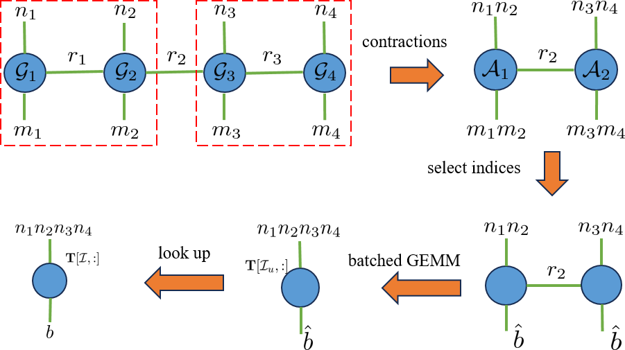
Figure 4: Optimized TTM embedding lookup.

Embedding tables are widely used to transfer discrete features into continuous hidden space. The row size of embedding tables is usually much larger than the column size, making TTM compression more suitable than the TT format. In the following, we use an order-4 TTM embedding table to illustrate how to accelerate the lookup process.

We consider an embedding table $\mathbf{T}\in\mathbb{R}^{m\times n}$. A look-up operation selects the submatrix $\mathbf{T}[\mathcal{I},:]\in\mathbb{R}^{b\times n}$ for the index set $\mathcal{I}=\{i_{k}\}_{k=1}^{b}$. This operation is fast and inexpensive. However, the full embedding table itself is extremely memory-consuming. Suppose that $m=m_{1}m_{2}m_{3}m_{4},n=n_{1}n_{2}n_{3}n_{4}$, then we reshape $\mathbf{T}$ into tensor $\mathbfcal{T}\in\mathbb{R}^{m_{1}\times n_{1}\times\cdots\times m_{4}\times n_{4}}$ and represent it in TTM format

$$\mathbfcal{T}=\mathbfcal{G}_{1}\times_{4,1}\mathbfcal{G}_{2}\times_{4,1}\mathbfcal{G}_{3}\times_{4,1}\mathbfcal{G}_{4}.$$ (15)

The compressed embedding table does not have the matrix $\mathbf{T}$ explicitly. We convert each row index $i_{k}\in\mathcal{I}$ to a tensor index vector $(z_{1}^{k},z_{2}^{k},z_{3}^{k},z_{4}^{k})$ and denote $\mathcal{Z}_{t}=\{z_{t}^{k}\}_{k=1}^{b}$, then $\mathbf{T}[\mathcal{I},:]$ can be computed by contracting the tensors $\{\mathbfcal{G}_{t}[:,\mathcal{Z}_{t},:,:]\}_{t=1}^{4}$ where each has size $r_{t-1}\times b\times n_{i}\times n_{t}$. The $\mathbfcal{G}_{t}[:,\mathcal{Z}_{t},:,:]$ stores many duplicated values especially when the set $\mathcal{I}$ is large. Therefore, directly computing the tensor contractions can cause much computing and memory overhead.

We optimize the tensor contraction by eliminating the redundant computation at two levels. Row-index level. We construct the index set $\mathcal{I}_{u}=\{i_{k}\}_{k=1}^{\hat{b}}$ containing all unique indices in $\mathcal{I}$. We can easily obtain $\mathbf{T}[\mathcal{I},:]$ from $\mathbf{T}[\mathcal{I}_{u},:]$. Tensor-index level. The reduced row index set $\mathcal{I}_{u}$ leads to $\hat{b}$ associated tensor index vectors $(z_{1}^{k},z_{2}^{k},z_{3}^{k},z_{4}^{k})$, but at most $m_{1}m_{2}$ pairs of $(z_{1}^{k},z_{2}^{k})$ and $m_{3}m_{4}$ pairs of $(z_{3}^{k},z_{4}^{k})$ are unique. Therefore, we can consider all unique pairs $(z_{1}^{k},z_{2}^{k})$ and $(z_{3},z_{4})$ and compute

$$\mathbfcal{A}_{1}= \mbox{\bf einsum}(r_{0}m_{1}n_{1}r_{1},r_{1}m_{2}n_{2}r_{2}\Rightarrow(m_{1}m_{2})(n_{1}n_{2})r_{2},[\mathbfcal{G}_{1},\mathbfcal{G}_{2}]),$$ (16)

$$\mathbfcal{A}_{2}= \mbox{\bf einsum}(r_{2}m_{3}n_{3}r_{3},r_{3}m_{4}n_{4}r_{4}\Rightarrow r_{2}(m_{3}m_{4})(n_{3}n_{4}),[\mathbfcal{G}_{3},\mathbfcal{G}_{4}]).$$ (17)

For each $i_{k}\in\mathcal{I}_{u}$, let $(j_{1}^{k},j_{2}^{k})$ be the coordinate of $i_{k}$ for size $(m_{1}m_{2},m_{3}m_{4})$. We denote $\mathcal{J}_{1}=\{j_{1}^{k}\}_{k=1}^{\hat{b}}$ and $\mathcal{J}_{2}=\{j_{2}^{k}\}_{k=1}^{\hat{b}}$, then compute the unique rows of $\mathbf{T}$ as

$$\mathbf{T}[\mathcal{I}_{u},:]=\mbox{\bf einsum}(\hat{b}(n_{1}n_{2})r_{2},r_{2}\hat{b}(n_{3}n_{4})\Rightarrow\hat{b}(n_{1}n_{2}n_{3}n_{4}),[\mathbfcal{A}_{1}[\mathcal{J}_{1},:,:],\mathbfcal{A}_{1}[:,\mathcal{J}_{2},:]]).$$ (18)

Figure 4 summarizes the whole process of TTM embedding table look up. This approach can be easily applied to higher-order embedding tables by first grouping some small tensor cores to obtain intermediate tensors and then utilizing them to compute unique row vectors.

Performance.

We demonstrate the optimized TTM embedding tables on a single RTX 3090 GPU. We consider an embedding table of TTM shape $[[80,50,54,50],[4,4,6,8]]$ and rank $32$, extracted from a practical DLRM model. As shown in Figure 5, our proposed method achieves about $4-5\times$ speed-up and $2-3\times$ memory saving than the standard TTM embedding without any optimization.

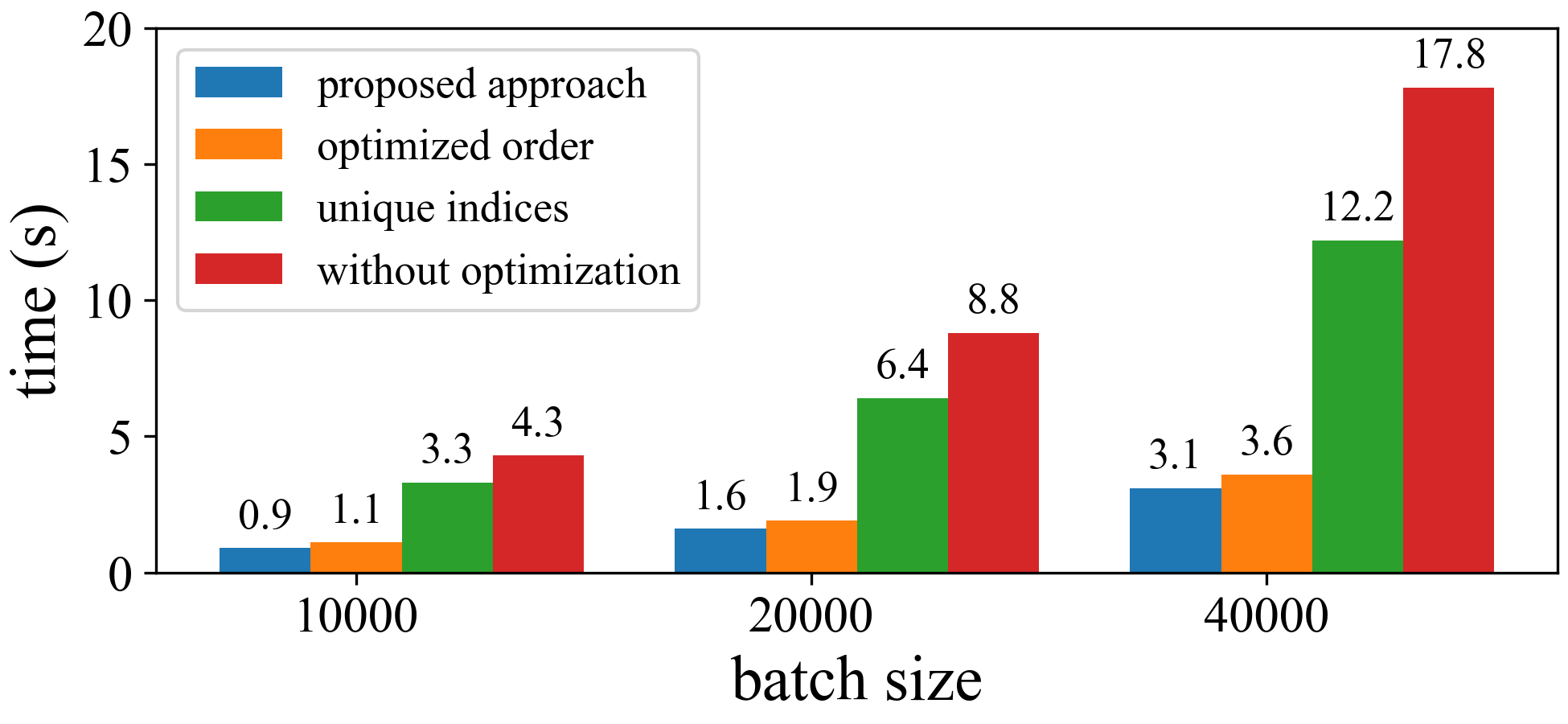
(a) Speed-up

(b) Memory reduction

Figure 5: Performance of optimized TTM embedding table lookup. The labels proposed approach, optimized order, unique indices, without optimization represent the new method in 4.1, the method that only uses the unique order, the method that only uses the unique indices, and the method without optimization, respectively.

4.2 Contraction Path Optimization for TT-Vector Multiplications

Next, we optimize the forward- and back- propagation of linear layers in the TT format. We consider the linear layer $\mathbf{Y}=\mathbf{X}\mathbf{W}$, where $\mathbf{Y}\in\mathbb{R}^{b\times N_{2}},\mathbf{W}\in\mathbb{R}^{N_{1}\times N_{2}},\mathbf{X}\in\mathbb{R}^{b\times N_{1}}$. The $\mathbf{W}$ is compressed into the Tensor-Train format: $\mathbfcal{W}=[\![\mathbfcal{G}_{1},\ldots,\mathbfcal{G}_{2d}]\!]\in\mathbb{R}^{n_{1}\times\cdots\times n_{2d}}$,where $\mathbfcal{G}_{i}\in\mathbb{R}^{r_{i-1}\times n_{i}\times r_{i}}$ and $N_{1}=n_{1}\cdots n_{d},N_{2}=n_{d+1}\cdots n_{2d}$. The forward-propagation in the einsum form is

$$\mathbf{Y}=\mathbf{X}\mathbf{W}=\mbox{\bf einsum}(bn_{1}\ldots n_{d},S_{1},\ldots,S_{2d}\Rightarrow bn_{d+1}\ldots n_{2d},[\mathbfcal{X},\mathbfcal{G}_{1},\ldots,\mathbfcal{G}_{2d}])$$ (19)

where $\mathbfcal{X}\in\mathbb{R}^{b\times n_{1}\times\cdots\times n_{d}}$ is the reshaping of $\mathbf{X}$ and $S_{i}$ denotes $r_{i-1}n_{i}r_{i}$. Suppose that the gradient to $\mathbf{Y}$ is $\mathbf{g}_{\mathbf{Y}}$, then the gradients to $\mathbfcal{G}_{i}$ and $\mathbfcal{X}$ can be computed as follows:

$$\mathbf{g}_{\mathbfcal{G}_{i}} =\mbox{\bf einsum}\big{(}bn_{1}\ldots n_{d},bn_{d+1}\ldots n_{2d},S_{1},\ldots,S_{i-1},S_{i+1},\ldots,S_{2d}\Rightarrow S_{i},$$

$$\quad\quad\quad\quad\quad\quad\quad\quad\quad\quad\quad\quad\quad\,[\mathbfcal{X},\mathbf{g}{Y},\mathbfcal{G}_{1},\ldots,\mathbfcal{G}_{i-1},\mathbfcal{G}_{i+1},\ldots,\mathbfcal{G}_{2d}]),$$ (20)

$$\mathbf{g}_{\mathbfcal{X}} =\mbox{\bf einsum}\big{(}bn_{d+1}\ldots n_{2d},S_{1},\ldots,S_{2d}\Rightarrow bn_{1}\ldots n_{d},[\mathbf{g}{Y},\mathbfcal{G}_{1},\ldots,\mathbfcal{G}_{2d}]).$$ (21)

In total, $2d+2$ contraction sequences are needed for the TT-format forward- and back- propagation. To reduce the computational costs, it is critical to find an optimal or near-optimal contraction path.

Large batch case.

We denote $\mathbfcal{A}_{i}:=\mathbfcal{G}_{1}\times\cdots\times\mathbfcal{G}_{i},\mathbfcal{A}_{-i}=\mathbfcal{G}_{d-i+1}\times\cdots\times\mathbfcal{G}_{d},\mathbfcal{B}_{i}:=\mathbfcal{G}_{d+1}\times\cdots\times\mathbfcal{G}_{d+i},\mathbfcal{B}_{-i}=\mathbfcal{G}_{2d-i+1}\times\cdots\times\mathbfcal{G}_{2d}$, which are all computed sequentially. In practice, we only need to compute $\mathbfcal{A}_{d},\mathbfcal{A}_{-d},\mathbfcal{B}_{d},\mathbfcal{B}_{-d}$ and store the intermediate results. The forward-propagation (19) is then computed in the following way

$$\mathbfcal{T}_{1} = \mbox{\bf einsum}(bn_{1}\ldots n_{d},n_{1}\ldots n_{d}r_{d}\Rightarrow br_{d},[\mathbfcal{X},\mathbfcal{A}_{d}])$$ (22)

$$\mathbfcal{Y} = \mbox{\bf einsum}(br_{d},r_{d}n_{d+1}\ldots n_{2d}\Rightarrow bn_{1}\ldots n_{d},[\mathbfcal{T}_{1},\mathbfcal{B}_{d}]).$$ (23)

In backward propagation, the gradients are computed in the following way:

• The gradient $\mathbf{g}{X}$ is computed as

  $$\mathbfcal{U}_{1} = \mbox{\bf einsum}(bn_{d+1}\ldots n_{2d},r_{d}n_{d+1}\ldots n_{2d}\Rightarrow br_{d},[\mathbf{g}_{\mathbfcal{Y}},\mathbfcal{B}_{d}])$$ (24)

  $$\mathbf{g}{X} = \mbox{\bf einsum}(br_{d},n_{1}\ldots n_{d}r_{d}\Rightarrow bn_{1}\ldots n_{d},[\mathbfcal{U}_{1},\mathbfcal{A}_{d}]).$$ (25)

• The gradients $\mathbf{g}_{\mathbfcal{G}_{i}}$ for $i\geq d+1$ can be computed as

  $$\mathbfcal{T}_{2} = \mbox{\bf einsum}(br_{d},bn_{d+1}\ldots n_{2d}\Rightarrow r_{d}n_{d+1}\ldots n_{2d},[\mathbfcal{T}_{1},\mathbf{g}_{\mathbfcal{Y}}])$$ (26)

  $$\mathbf{g}_{\mathbfcal{G}_{i}} = \mbox{\bf einsum}(r_{d}n_{d+1}\ldots n_{2d},r_{d}n_{d+1}\ldots n_{i-1}r_{i-1},r_{i}n_{i+1}\ldots n_{2d}\Rightarrow$$

  $$r_{i-1}n_{i}r_{i},\;[\mathbfcal{T}_{2},\mathbfcal{B}_{i-1-d},\mathbfcal{B}_{-(2d-i)}]).$$

• Similarly, the gradients $\mathbf{g}_{\mathbfcal{G}_{i}}$ for $i\leq d$ can be computed as

  $$\mathbfcal{U}_{2} = \mbox{\bf einsum}(br_{d},bn_{1}\ldots n_{d}\Rightarrow r_{d}n_{1}\ldots n_{d},[\mathbfcal{U}_{1},\mathbfcal{X}])$$ (28)

  $$\mathbf{g}_{\mathbfcal{G}_{i}} = \mbox{\bf einsum}(r_{d}n_{1}\ldots n_{d},n_{1}\ldots n_{i-1}r_{i-1},r_{i}n_{i+1}\ldots n_{d}r_{d}\Rightarrow$$

  $$r_{i-1}n_{i}r_{i},\;[\mathbfcal{U}_{2},\mathbfcal{A}_{i},\mathbfcal{A}_{-(d-i)}]).$$

The contraction paths of forward- and back- propagation are summarized in Appendix A.4.

Analysis.

The proposed empirical path is near-optimal for large batch sizes. The following result analyzes the contraction path for forward-propagation.

Proposition 4.1.

Suppose that the TT ranks satisfy $1=r_{0}<r_{1}\leq\cdots\leq r_{d}\geq r_{d-1}>\cdots\geq r_{2d}=1$ and the batch size $b$ is large enough. There exist groups $\{S_{i}\}_{i=1}^{k}$ where $S_{i}=\{\mathbfcal{G}_{j_{i}+1},\ldots,\mathbfcal{G}_{j_{i+1}}\}$ containing consecutive tensor cores for $0=j_{1}<\cdots<j_{k}<j_{k+1}=2d$. Then, the contraction path with the least number of flops for the forward-propagation (19) first contracts the tensor cores in each $S_{i}$ to obtain $\mathbfcal{V}_{i}$ with dimension $r_{j_{i}}\times n_{j_{i}+1}\times\cdots\times n_{j_{i+1}}\times r_{j_{i+1}}$ and then contract the input tensor $\mathbfcal{X}$ with tensors $\{\mathbfcal{V}_{i}\}_{i=1}^{k}$ in the sequential order.

Proof.

See Appendix A.3 for the complete proof. ∎

Proposition 4.1 implies that the optimal path first contracts some consecutive tensor cores and then contracts obtained tensors with the input tensor sequentially. The groups $\{S_{i}\}_{i=1}^{k}$ depend on the dimensions, ranks, and batch size. The proposed contraction path satisfies the property shown in Proposition 4.1 and has flops roughly $b(n_{1}\cdots n_{d}+n_{d+1}\cdots n_{2d})r_{d}$. The optimal contraction path has flops about $bn_{1}\cdots n_{d}c_{1}+bn_{d+1}\cdots n_{2d}c_{2}$, where $c_{1},c_{2}$ are some constants. Hence, the proposed is near-optimal and has a comparable complexity to the optimal path. Suppose the optimal path is different from the proposed empirical path. Then the optimal path will likely involve a few more large intermediate tensors, which pose more memory costs during training and inference especially for static computational graphs. The empirical path is a good choice to balance time and memory consumption. Similar arguments can be applied to the contractions for back-propagation.

When the batch size is small, the optimal path may have much fewer flops. However, the execution time is almost the same as the proposed path since all the operations are too small. Hence, we can use the proposed path for most batch sizes. See Appendix A.5 for more analysis.

4.3 GPU Performance Optimization via CUDA Graph

While CoMERA consumes much less computing FLOPS than standard uncompressed training, it can be slower on GPU if not implemented carefully. Therefore, it is crucial to optimize the GPU performance to achieve real speedup. Modern GPUs are highly optimized for large-size matrix multiplications. However, the small-size tensor contractions in CoMERA are not yet optimized on GPU and require many small-size GPU kernels, causing significant runtime overhead. During the training, Cuda Graph launches and executes the whole computing graph rather than launching a large number of kernels sequentially. This can eliminate lots of back-end overhead and lead to significant training speedup. We remark that this is just an initial step of GPU optimization. We expect that a more dedicated GPU optimization can achieve a more significant training speedup.

Table 1: Result of Transformer on MNLI of batch size 128.

	validation	total size (MB)	compressed size (MB)
uncompressed training	62.2%	256 ($1\times$)	253 ($1\times$)
CoMERA (early stage)	63.3%	5.9 ($43\times$)	3.4 ($74\times$)
CoMERA (late stage), target ratio: 0.8	62.2%	4.9 ($52\times$)	2.4 ($105\times$)
CoMERA (late stage), target ratio: 0.5	62.1%	3.9 ($65\times$)	1.4 ($181\times$)
CoMERA (late stage), target ratio: 0.2	61.5%	3.2 ($80\times$)	0.7 ($361\times$)

5 End-to-End Training Results

In this section, we test the performance of CoMERA on a transformer and a DLRM benchmark. Our experiments are run on a Nvidia RTX 3090 GPU with 24GB RAM.

5.1 A Medium-Size Transformer with Six Encoders

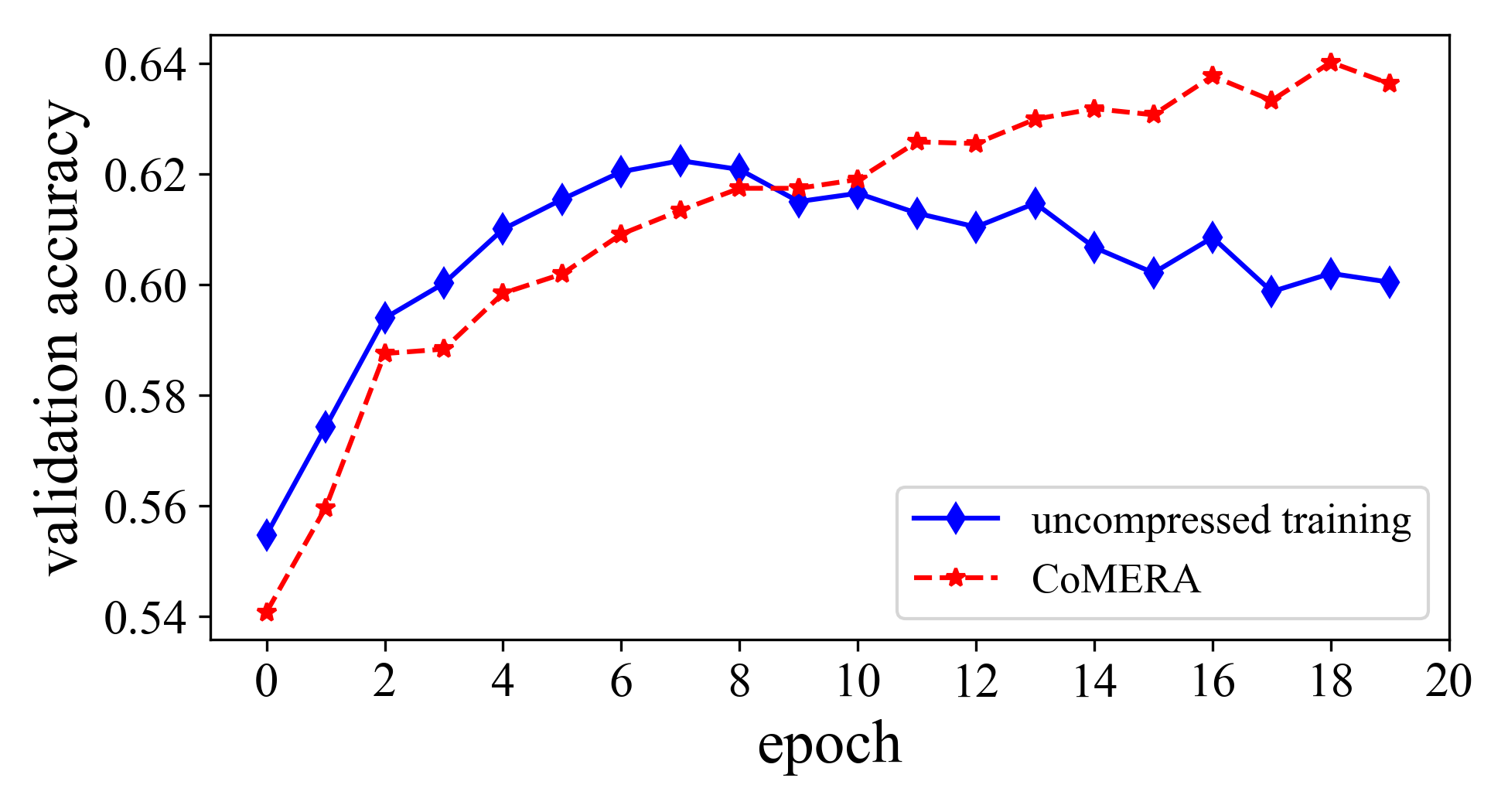
Figure 6: Behavior of early-stage CoMERA training on the MNLI dataset.

We first consider a six-encoder transformer. The embedding tables and all linear layers are represented as tensor cores in the training process as detailed in Appendix A.6. We train this model on the MNLI dataset [34] with the maximum sequence length $128$ and compare the accuracy, resulting model size, and training time of CoMERA with the standard uncompressed training.

Table 2: The change of ranks of layers in the fifth encoder block.

	before training	early-stage rank	late-stage rank
Q-layer in attention	$(12,30,30,30,12)$	$(12,30,30,30,12)$	$(0,0,0,0,0)$
K-layer in attention	$(12,30,30,30,12)$	$(12,30,30,30,12)$	$(0,0,0,0,0)$
V-layer in attention	$(12,30,30,30,12)$	$(12,30,30,30,12)$	$(9,11,11,7,9)$
FC-layer in attention	$(12,30,30,30,12)$	$(12,30,29,30,12)$	$(9,8,10,8,8)$
#1 linear-layer in Feed-Forward	$(12,30,30,30,16)$	$(0,0,0,0,0)$	$(0,0,0,0,0)$
#2 linear-layer in Feed-Forward	$(16,30,30,30,12)$	$(0,0,0,0,0)$	$(0,0,0,0,0)$

CoMERA Accuracy and Compression Performance.

Table 1 summarizes the training results. The early-stage training of CoMERA achieves $74\times$ compression ratio on all tensorized layers, and the validation accuracy is even higher than the uncompressed training. Figure 6 shows the validation accuracy of CoMERA. In the late stage of CoMERA, we set different target compression ratios for more aggressive rank pruning. The target compression ratios are for the tensorized layers rather than for the whole model. The late-stage training can reach the desired compression ratio with very little accuracy drop. The smallest model has a compression ratio of $80\times$ for the whole model due to a $361\times$ compression on the tensorized layers with slightly worse accuracy.

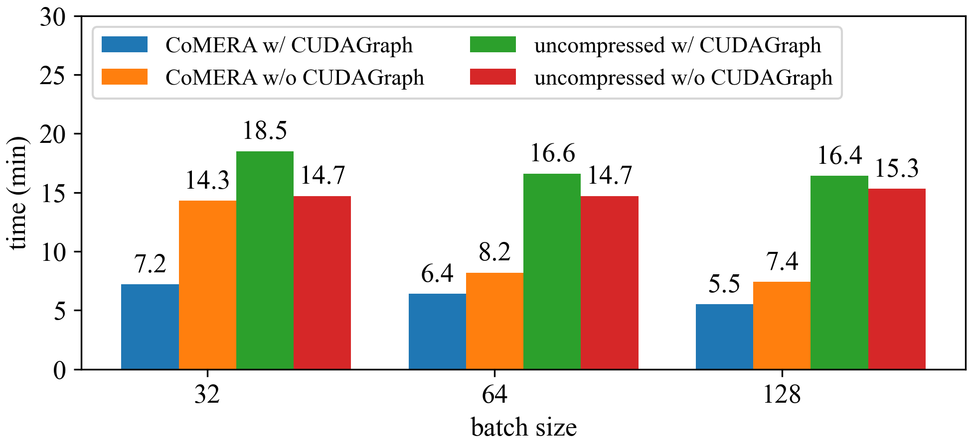
Figure 7: Training time per epoch for the six-encoder transformer model on the MNLI dataset.

Architecture Search Capability of CoMERA.

A major challenge in training is architecture search: shall we keep certain layers of a model? Interestingly, CoMERA has some capability of automatic architecture search. Specifically, the ranks of some layers become zero in the training, and thus the whole layer can be removed. For the target compression ratio $0.2$, the whole second last encoder and some linear layers in other encoders are completely removed after late-stage rank-adaptive training. The change of ranks of layers in the 5th encoder is shown in Table 2.

Training Time.

As shown in Figure 7, CoMERA with CUDAGraph achieves around $3\times$ speed-up than uncompressed training. CoMERA without CUDAGraph can take much longer time in small batch-size setting due to the launching overhead of too many small kernels. The uncompressed training with CUDAGraph takes longer time than the one without CUDAGraph. This is because CUDAGraph requires all batches to have the same sequence length, and the consequent computing overhead is more than the time reduction of CUDAGraph. In contrary, CoMERA has much fewer computing FLOPS and the computing part accounts for a much smaller portion of the overall runtime.

5.2 A DLRM Model with 4-GB Model Size

We further test CoMERA on DLRM [28] released by Meta on Criteo Ad Kaggle dataset [19]. We compress the ten largest embedding tables into the TTM format as in Section 4.1. All fully connected layers with sizes $>128$ are compressed into TT format. The model is trained for two epochs.

Effect of Optimized TTM Embedding.

The training time per epoch and peak memory consumption are shown in Figure 8. Our optimized TTM lookup speeds up the training process by around $2\times$ and remarkably reduces the memory cost by $4-5\times$, especially for large batch training.

Overall Performance of CoMERA.

Table 3 shows the testing accuracy, testing loss (measured as normalized CE), memory costs, and model sizes of CoMERA and uncompressed training. CoMERA achieves similar accuracy as the uncompressed training. Furthermore, CoMERA compresses the whole DLRM model by $99\times$ and saves $7\times$ peak memory cost (with consideration of the data and backend overhead in a large-batch setting) in the training process. The reduction of model size and memory cost mainly comes from the compact TTM tensor representation of large embedding tables.

Table 3: Training results on the DLRM model with a batch size $10,000$.

	uncompressed	CoMERA
accuracy	78.68%	78.76%
normalized CE	0.793	0.792
model size (GB)	4.081	0.041 (99$\times$)
peak memory (GB)	18.275	2.612 (7$\times$)

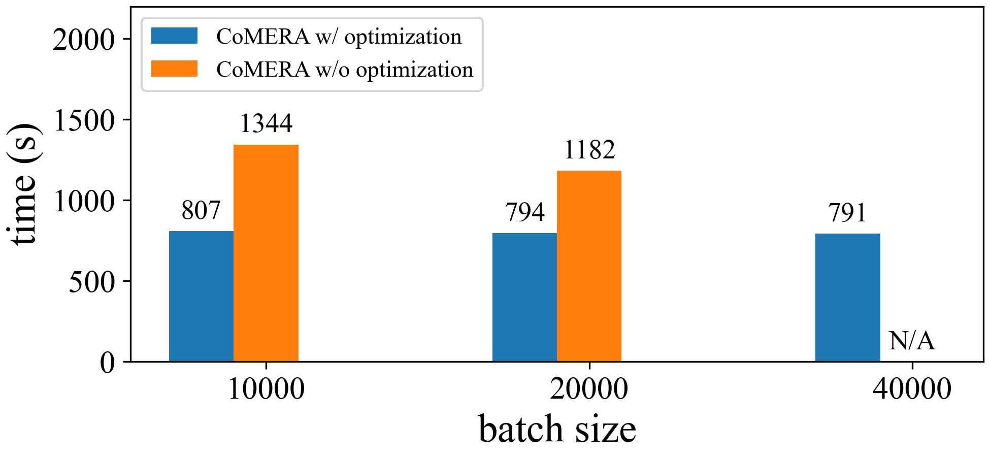
(a) Training time per epoch.

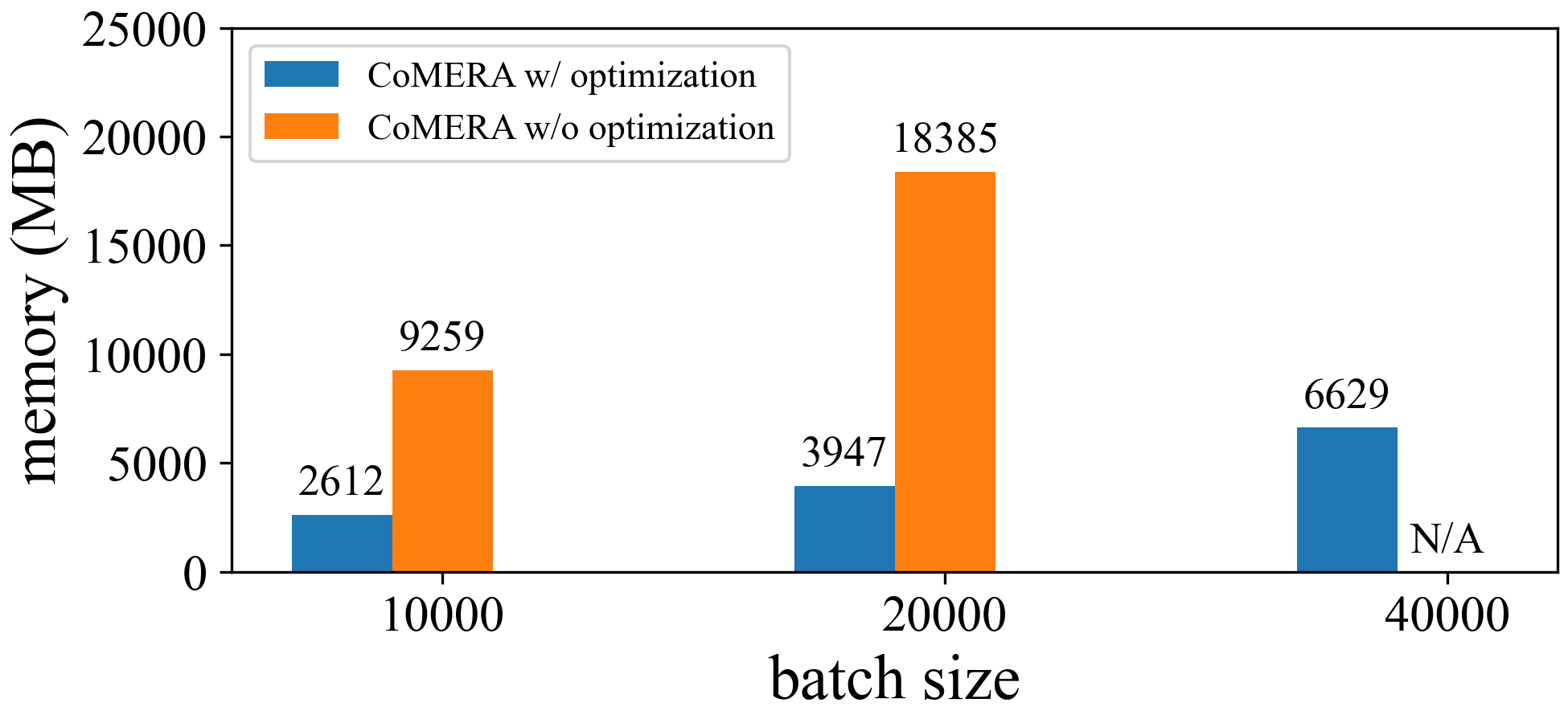
(b) Memory cost.

Figure 8: Performance of optimized CoMERA on training DLRM.

5.3 Comparison with GaLore and LTE

We compare our method with two recent low-rank compressed training frameworks: GaLore  [37] and LTE [17]. GaLore [37] reduces the memory cost by performing SVD compression on the gradient, and LTE represents the weights as the sum of parallel low-rank matrix factorizations. We evaluate their memory costs and training times per epoch on the six-encoder transformer model under different batch sizes. We do not compare the total training time because the training epochs of various methods are highly case-dependent.

Training Time Per Epoch.

We use rank $128$ for the low-rank gradients in GoLore, and rank $32$ and head number $16$ for the low-rank adapters in LTE. For a fair comparison, all methods are executed with CUDA graph to reduce the overhead of launching CUDA kernels. The runtimes per training epochs are reported in Figure 1(a). For the LTE, we only report the results for batch sizes $32,64,128$ since it requires the batch size to be a multiple of the head number. Overall, our CoMERA is about $2\times$ faster than GaLore and $3\times$ faster than LTE for all batch sizes, because the forward and backward propagation using low-rank tensor-network contractions dramatically reduce the computing FLOPS.

Memory Cost.

Figure 1 (b) shows the memory cost of all three training methods. In the single-batch setting as used in [37], our CoMERA method is $9\times$ more memory-efficient than Galore on the tested case (with consideration of data and back-end cost). As the batch size increases, the memory overhead caused by data and activation functions becomes more significant, leading to less memory reduction ratios. However, our proposed CoMERA still uses the least memory.

6 Conclusions and Future work

This work has presented CoMERA framework to reduce the memory and computing time of training AI models. We have investigated rank-adaptive training via multi-objective optimization to meet specific model sizes while maintaining model performance. We have achieved real training speedup on GPU via three optimizations: optimizing the tensorized embedding tables, optimizing the contraction path in tensorized forward and backward propagation, and optimizing the GPU latency via CUDAGraph. The experiments on a transformer model demonstrated that CoMERA can achieve $2-3\times$ speedup per training epoch. The model sizes of the transformer and a DLRM model have been reduced by $43\times$ to $99\times$ in the training process, leading to significant peak memory reduction (e.g., $7\times$ total reduction in large-batch training of DLRM on a single GPU). Our method has also outperformed the latest GaLore and LTE frameworks in both memory and runtime efficiency. We have also observed further speedup by combining CoMERA with mixed-precision computation. The discussions and some preliminary results are in Appendix A.7.

Unlike large-size matrix operations, the small low-rank tensor operations used in CoMERA are not yet well-supported by existing GPU kernels. The performance of CoMERA can be further boosted significantly after a comprehensive GPU optimization. The existing optimizers, e.g. Adam, are well-studied for uncompressed training. However, CoMERA has a very different optimization landscape due to the tensorized structure. Therefore, it is also worth studying the optimization algorithms specifically for CoMERA in the future.

Appendix A Supplementary Material

A.1 Proof of Proposition 3.1

Proof.

The objective function in (9) is bounded below by $0$. Hence, the problem (9) has a finite infimum value $f^{*}$. Let $\{\mathbfcal{G}^{k},\mathbf{D}^{k}\}_{k=1}^{\infty}$ be a sequence such that $\lim_{k\to\infty}L(\mathbfcal{G}^{k},\mathbf{D}^{k})+\gamma\hat{S}(\mathbf{D}^{k})+\beta\|\mathbfcal{G}^{k}\|^{2}=f^{*}$. The sequence must be bounded because of the $l_{1}$ regularization of $\mathbf{D}$ and the $\ell_{2}$ regularization of $\mathbfcal{G}$. As a result, the sequence has a cluster point $(\mathbfcal{G}^{*},\mathbf{D}^{*})$ which is a minimizer of the (9). Let $C:=\|\mathbfcal{G}^{*}\|^{2}$. The relaxation (9) is equivalent to the constrained optimization problem.

$$\min_{\mathbfcal{G},\mathbf{D}} L(\mathbfcal{G},\mathbf{D})+\gamma\hat{S}(\mathbf{D})$$ (30)

s.t. $$\|\mathbfcal{G}\|^{2}\leq C.$$

It implies that the solution to the training problem (9) is a Pareto point of the multi-objective optimization problem $\min_{\mathbfcal{G},\mathbf{D}}(L(\mathbfcal{G},\mathbf{D}),\hat{S}(\mathbf{D}))$. ∎

A.2 Algorithm for Late Stage Optimization in Section 3.2

The algorithm for the late stage optimization in Section 3.2 is summarized in Algorithm 1.

Algorithm 1 Solve relaxed scalarization problem (12)

Input: Initializations $\mathbfcal{G}_{0},\mathbf{D}_{0}$, constants $L_{0},S_{0},w_{1},w_{2},\rho,\beta$, and an optimization algorithm $\mathcal{O}$.
      Output: Tensor cores $\mathbfcal{G}_{T}$ and rank-control parameters $\mathbf{D}_{T}$.

for $t=0,\ldots,T-1$ do

     if $w_{1}(L(\mathbfcal{G}_{t},\mathbf{D}_{t})-L_{0})\geq w_{2}({S}(\mathbf{D}_{t})-S_{0})$ then

         The optimization algorithm $\mathcal{O}$ runs one step on the problem (13).

     else

         The optimization algorithm $\mathcal{O}$ runs one step on the problem (14).

     end if

end for

A.3 Proof of Proposition 4.1

Proof.

For convenience, let $V_{i}$ be a string of characters to specify the dimension of $\mathbfcal{V}_{i}$, $C_{i}$ be the set of tensor cores used to obtain $\mathbfcal{V}_{i}$, and $\mathbfcal{X}_{i}$ be the tensor by contracting $\mathbfcal{X}$ with $\mathbfcal{V}_{1},\ldots.\mathbfcal{V}_{i}$, denoted by the string $X_{i}$.

We first show that $\mathbfcal{V}_{1}$ must be in the proposed format. Suppose otherwise for contradiction. Let $\mathbfcal{G}_{i}$ be the first tensor core used to obtain $\mathbfcal{V}_{1}$. If $i=1$, then we write $V_{1}={V}_{1}^{1}{V}_{1}^{2}$ where the tensor $\mathbfcal{V}_{1}^{1}$ corresponding to $V_{1}^{1}$ is obtained by contractions of longest consecutive tensor cores containing $\mathbfcal{G}_{i}$ in the set $C_{1}$. Let $Z_{1}={V}_{i}^{1}\cap\tilde{X}$, $Z_{2}={V}_{i}^{2}\cap\tilde{X}$. The number of flops for the contraction between $\mathbfcal{\widetilde{X}}$ and $\mathbfcal{V}_{1}$ is $\frac{\pi(X)\pi(V_{1}^{1})\pi(V_{1}^{2})}{\pi(Z_{1})\pi(Z_{2})}$. If we first contract $\mathbfcal{\widetilde{X}}$ with $\mathbfcal{V}_{1}^{1}$ and then contract the obtained tensor with $\mathbfcal{V}_{1}^{2}$, the number of flops is $\frac{\pi(X)\pi(V_{1}^{1})}{\pi(Z_{1})}+\frac{\pi(X)\pi(V_{1}^{1})\pi(V_{1}^{2})}{\pi(Z_{1})^{2}\pi(Z_{2})}$ which is less than $\frac{\pi(X)\pi(V_{1}^{1})\pi(V_{1}^{2})}{\pi(Z_{1})\pi(Z_{2})}$ since $Z_{2}\neq V_{1}^{2}$. It contradicts our assumption that this is the optimal path. If $d\geq i>1$, let $\mathbfcal{S}$ be the tensor generated by the longest consecutive tensor cores containing $\mathbfcal{G}_{i-1}$ and used in the optimal path. A better path is to first contract $\mathbfcal{V}_{1}$ with $\mathbfcal{S}$ to obtain $\mathbfcal{W}$, then contract $\mathbfcal{W}$ with $\mathbfcal{X}$ and all other unused parts in the optimal path. It is better because the number of flops for contracting $\mathbfcal{W}$ and $\mathbfcal{X}$ is no greater than that for contracting $\mathbfcal{V}_{1}$ and $\mathbfcal{X}$ and the new path reduces the number of flops in the remaining contractions. The reduction in the remaining contractions is more than the potential flop increase in obtaining $\mathbfcal{W}$ when the batch size $b$ is big enough. Finally, we consider the case that $i>d$. Let $\mathbfcal{G}_{j}$ be the first tensor core used to obtain $\mathbfcal{V}_{2}$. If $j>d$, then first contracting $\mathbfcal{V}_{1}$ and $\mathbfcal{V}_{2}$ and then all other parts is a better choice. Otherwise, if $j\leq d$, let $\mathbfcal{V}_{2}^{1}$ be the tensor contracted by the consecutive tensors containing $\mathbfcal{G}_{j}$ in $C_{2}$. The tensor $\mathbfcal{V}$ can be represented by the contraction of $\mathbfcal{V}_{2}^{1}$ and another tensor $\mathbfcal{V}_{2}^{2}$ generated by the remaining tensor cores in $C_{2}$. In this scenario, we can contract $\mathbfcal{V}_{2}^{1}$ with $\mathbfcal{V}_{1}$ to get $\mathbfcal{S}$, then $\mathbfcal{S}$ with $\mathbfcal{X}$ to get $\mathbfcal{W}$, then $\mathbfcal{V}_{2}^{2}$ with $\mathbfcal{W}$, and finally the obtained tensor with $\mathbfcal{V}_{3},\ldots,\mathbfcal{V}_{k}$. It is not hard to verify contracting $\mathbfcal{V}_{2}^{1}$ and $\mathbfcal{V}_{1}$, $\mathbfcal{S}$ and $\mathbfcal{S}$ and $\mathbfcal{X}$, and $\mathbfcal{W}$ and $\mathbfcal{V}_{2}^{2}$ uses less flops than directly contracting $\mathbfcal{X}$ with $\mathbfcal{V}_{1}$ and $\mathbfcal{V}_{2}$ directly when the batch size $b$ is large. Summarizing everything above, we can conclude that $\mathbfcal{V}_{1}$ must be in the proposed format.

The contraction of $\mathbfcal{X}_{i}$ and $\mathbfcal{V}_{i+1},\ldots,\mathbfcal{V}_{k}$ has the similar structure to the contraction of $\mathbfcal{X}$ and $\mathbfcal{V}_{1},\ldots,\mathbfcal{V}_{k}$. By applying the same proof, we conclude that the tensors $\mathbfcal{V}_{i}$’s must be in the format stated in the proposition and we will contract the input tensor $\mathbfcal{X}$ with the tensors $ten{V}_{1},\ldots,\mathbfcal{V}_{k}$ in the sequential order. ∎

A.4 Algorithm for Contraction Path in Section 4.2

The empirical near-optimal contraction path for tensor-compressed training is in Algorithm 2.

Algorithm 2 Empirical path for tensor-compressed forward- and back- propagation

Forward Input: Tensor cores $\mathbfcal{G}_{1},\ldots,\mathbfcal{G}_{2d}$ and input matrix $\mathbf{X}$.
Forward Output: Output matrix $\mathbf{Y}$, and intermediate results.

1:Reshape the matrix $\mathbf{X}$ to the tensor $\mathbfcal{X}$.

2:Compute $\mathbfcal{A}_{d},\mathbfcal{A}_{-d},\mathbfcal{B}_{d},\mathbfcal{B}_{-d}$ in the sequential order and store intermediate results of $\{\mathbfcal{A}_{i},\mathbfcal{A}_{-i},\mathbfcal{B}_{i},\mathbfcal{B}_{-i}\}_{i=1}^{d}$ for back-propagation.

3:Compute $\mathbfcal{T}_{1}$ as in (22) to store it for back-propagation.

4:Compute $\mathbfcal{Y}$ as in (23) and reshape it to the appropriate matrix $\mathbf{Y}$.

Backward Input: Inputs of Forward, stored results from Forward, and output gradient $\mathbf{g}_{\mathbf{Y}}$.
Backward Output: Gradients $\mathbf{g}_{\mathbf{X}},\mathbf{g}_{\mathbfcal{G}_{1}},\ldots,\mathbf{g}_{\mathbfcal{G}_{2d}}$.

1:Reshape the gradient $\mathbf{g}_{\mathbf{Y}}$ to the tensor $\mathbf{g}_{\mathbfcal{Y}}$.

2:Compute $\mathbfcal{U}_{1}$ and $\mathbf{g}_{\mathbfcal{X}}$ as in (24), (25) and store $\mathbfcal{U}_{1}$ for future use.

3:Compute $\mathbf{g}_{\mathbfcal{G}_{i}}$ for $i\geq d+1$ as in (26), (• ‣ 4.2) using stored tensors.

4:Compute $\mathbf{g}_{\mathbfcal{G}_{i}}$ for $i\leq d$ as in (22), (• ‣ 4.2) using stored tensors.

A.5 Small Batch Case for Contraction Path in Section 4.2

Small batch case.

The empirical contraction path in Algorithm 2 eliminates the batch size dimension $b$ early, so it is nearly optimal when the batch size is large. We may search for a better path using a greedy search algorithm to minimize the total operations. In each iteration, we prioritize the pairs that output the smallest tensors. Such a choice can quickly eliminate large intermediate dimensions to reduce the total number of operations. When the batch size is large, the searched path is almost identical to the empirical path in Algorithm 2 which eliminates the batch size dimension $b$ early. The searched path may differ from Algorithm 2 for small batch sizes, but their execution times on GPU are almost the same. This is because the tensor contractions for smaller batch sizes have a minor impact on the GPU running times. Consequently, despite certain tensor contractions in the empirical path being larger than those in the optimal path, the actual GPU execution times between them exhibit only negligible differences. Therefore, the empirical contraction path in Algorithm 2 is adopted for all batch sizes in CoMERA.

A.6 Compression Settings for the Experiment in Section 5.1

The compression settings for the experiment in Section 5.1 are shown in Table 4.

Table 4: Tensorized setting for the Transformer model in CoMERA.

	format	linear shape	tensor shape	rank
embedding	TTM	(30527,768)	(64,80,80,60)	30
attention	TT	(768,768)	(12,8,8,8,8,12)	30
feed-forward	TT	(768,3072)	(12,8,8,12,16,16)	30

A.7 Discussion: Mixed-Precision CoMERA

Modern GPUs offer low-precision computation to speed up the training and inference. It is natural to combine low-rank tensor compression and quantization to achieve the best training efficiency. However, CoMERA involves many small-size low-rank tensor contractions, and a naive low-precision implementation may even slow down the training due to the overhead caused by precision conversions.

To resolve the above issue, we implement mixed-precision computation in CoMERA based on one simple observation: large-size contractions enjoy much more benefits of low-precision computation than small-size ones. This is because the overhead caused by precision conversions can dominate the runtime in small-size contractions. In large-batch tensor-compressed training, small- and large-size tensor contractions can be distinguished by whether the batch size dimension $b$ is involved. In general, a contraction with the batch $b$ is regarded as large and is computed in a low precision. Otherwise, it is regarded small and is computed in full-precision. The actual mixed-precision algorithm depends on the contraction path used in the forward- and back- propagations of CoMERA.

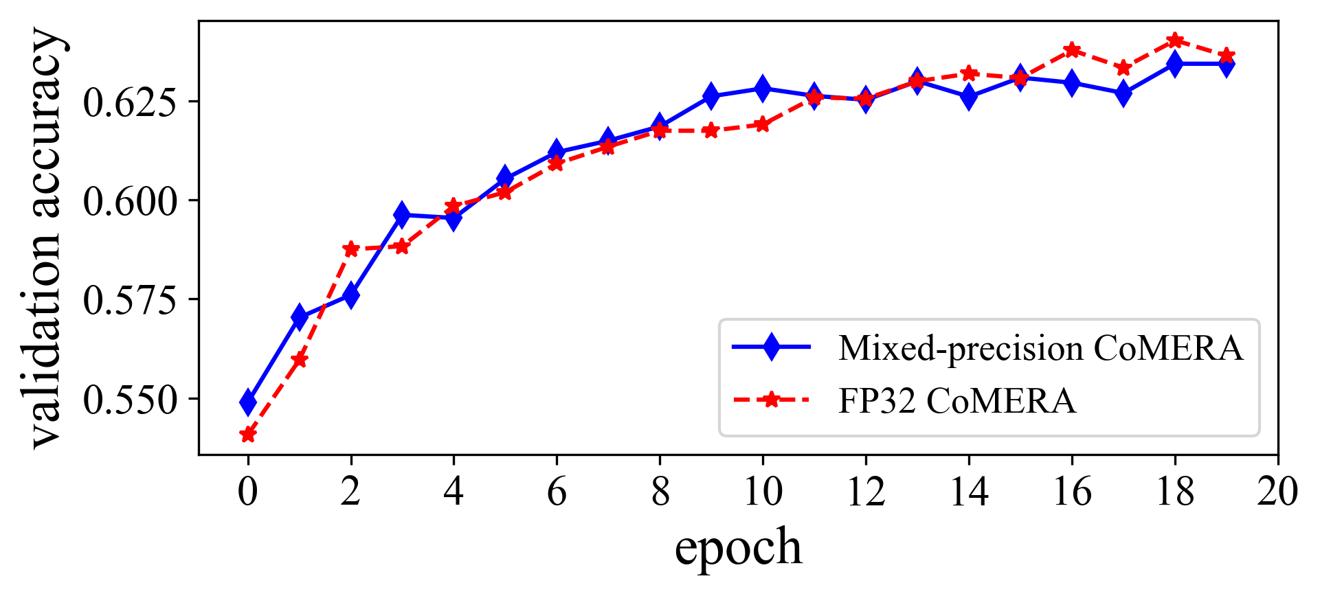
Figure 9: Convergence of mixed-precision CoMERA on the six-encoder transformer.

Runtime.

We evaluate the mixed-precision forward and backward propagations of CoMERA in a FP8 precision on the NVIDIA L4 GPU. We consider a single linear layer. The shapes $(1024,1024)$ and $(1024,4096)$ are converted to the TT shapes $(16,8,8,8,8,16)$ and $(16,8,8,16,16,16)$ respectively, and the ranks are both $32$. The total execution time for $1000$ forward and backward propagations are shown in Table 5. The FP8 tensor-compressed linear layer has about $3\times$ speed-up compared to the FP8 vanilla linear layer when the batch size and layer size are large. When the batch size is small, the FP8 vanilla linear layer is even faster. This is because the tensor-compressed linear layer consists of a few sequential computations that are not well supported by current GPU kernels. We expect to see a more significant acceleration after optimizing the GPU kernels.

Table 5: Speed-up of mixed-precision computation on tensor-compressed linear layers.

shape (b,m,n)	tensor-vector		matrix-vector
	FP8-mix	FP32	FP8	FP32
(10000,1024,1024)	1.95	1.63	1.02	2.82
(20000,1024,1024)	2.02	3.37	1.93	5.41
(40000,1024,1024)	2.55	6.82	4.27	10.93
(10000,1024,4096)	1.97	3.96	3.69	10.28
(20000,1024,4096)	2.96	8.32	7.26	20.93
(40000,1024,4096)	5.47	17.13	15.27	45.60

Table 6: Training results of mixed-precision CoMERA on DLRM (batch size=10,000).

	accuracy	normalized CE
FP32 CoMERA	78.76%	0.792
FP8/FP32 mixed-precision CoMERA	78.88%	0.793

Convergence.

We use the mixed-precision CoMERA to train the DLRM model and the six-encoder transformer. The result on DLRM is shown in Table 6. The convergence curve of the six-encoder transformer is shown in Figure 9. The experiments demonstrate that the accuracy of FP8 training is similar to FP32 training. However, we did not see much acceleration of using FP8 in the experiments. This is mainly because of ① the computation overhead of slow data type casting between FP32 and FP8; ② the sequential execution of small tensor contractions that are not well supported by current GPUs; ③ the relatively small sizes of linear layers in the tested models. We will investigate these problems in the future, and are optimistic to see significant acceleration on larger models.

References

- [1] AI and compute. https://openai.com/blog/ai-and-compute/. OpenAI in 2019.
- [2] ChatGPT and generative AI are booming, but the costs can be extraordinary. https://www.cnbc.com/2023/03/13/chatgpt-and-generative-ai-are-booming-but-at-a-very-expensive-price.html. Accessed: 2023-03-15.
- [3] Update: ChatGPT runs 10K Nvidia training GPUs with potential for thousands more. https://www.fierceelectronics.com/sensors/chatgpt-runs-10k-nvidia-training-gpus-potential-thousands-more. Accessed: 2023-03-15.
- [4] Tom B Brown, Benjamin Mann, Nick Ryder, Melanie Subbiah, Jared Kaplan, Prafulla Dhariwal, Arvind Neelakantan, Pranav Shyam, Girish Sastry, Amanda Askell, et al. Language models are few-shot learners. arXiv preprint arXiv:2005.14165, 2020.
- [5] Giuseppe G Calvi, Ahmad Moniri, Mahmoud Mahfouz, Qibin Zhao, and Danilo P Mandic. Compression and interpretability of deep neural networks via tucker tensor layer. arXiv:1903.06133, 2019.
- [6] Beidi Chen, Tri Dao, Kaizhao Liang, Jiaming Yang, Zhao Song, Atri Rudra, and Christopher Re. Pixelated Butterfly: Simple and efficient sparse training for neural network models. arXiv preprint arXiv:2112.00029, 2021.
- [7] Wenlin Chen, James Wilson, Stephen Tyree, Kilian Weinberger, and Yixin Chen. Compressing neural networks with the hashing trick. In International Conference on Machine Learning, pages 2285–2294, 2015.
- [8] Kalyanmoy Deb, Karthik Sindhya, and Jussi Hakanen. Multi-objective optimization. In Decision sciences, pages 161–200. CRC Press, 2016.
- [9] Suyog Gupta, Ankur Agrawal, Kailash Gopalakrishnan, and Pritish Narayanan. Deep learning with limited numerical precision. In International Conference on Machine Learning, pages 1737–1746, 2015.
- [10] Song Han, Huizi Mao, and William J Dally. Deep compression: Compressing deep neural networks with pruning, trained quantization and huffman coding. arXiv preprint arXiv:1510.00149, 2015.
- [11] Cole Hawkins, Xing Liu, and Zheng Zhang. Towards compact neural networks via end-to-end training: A bayesian tensor approach with automatic rank determination. SIAM Journal on Mathematics of Data Science, 4(1):46–71, 2022.
- [12] Cole Hawkins and Zheng Zhang. Bayesian tensorized neural networks with automatic rank selection. Neurocomputing, 453:172–180, 2021.
- [13] Qinyao He, He Wen, Shuchang Zhou, Yuxin Wu, Cong Yao, Xinyu Zhou, and Yuheng Zou. Effective quantization methods for recurrent neural networks. arXiv preprint arXiv:1611.10176, 2016.
- [14] Geoffrey Hinton, Oriol Vinyals, and Jeff Dean. Distilling the knowledge in a neural network. arXiv preprint arXiv:1503.02531, 2015.
- [15] Oleksii Hrinchuk, Valentin Khrulkov, Leyla Mirvakhabova, Elena Orlova, and Ivan Oseledets. Tensorized embedding layers for efficient model compression. arXiv preprint arXiv:1901.10787, 2019.
- [16] Itay Hubara, Matthieu Courbariaux, Daniel Soudry, Ran El-Yaniv, and Yoshua Bengio. Quantized neural networks: Training neural networks with low precision weights and activations. The Journal of Machine Learning Research, 18(1):6869–6898, 2017.
- [17] Minyoung Huh, Brian Cheung, Jeremy Bernstein, Phillip Isola, and Pulkit Agrawal. Training neural networks from scratch with parallel low-rank adapters. arXiv preprint arXiv:2402.16828, 2024.
- [18] Max Jaderberg, Andrea Vedaldi, and Andrew Zisserman. Speeding up convolutional neural networks with low rank expansions. arXiv preprint arXiv:1405.3866, 2014.
- [19] Olivier Chapelle Jean-Baptiste Tien, joycenv. Display advertising challenge, 2014.
- [20] Valentin Khrulkov, Oleksii Hrinchuk, Leyla Mirvakhabova, and Ivan Oseledets. Tensorized embedding layers for efficient model compression. arXiv preprint arXiv:1901.10787, 2019.
- [21] Yong-Deok Kim, Eunhyeok Park, Sungjoo Yoo, Taelim Choi, Lu Yang, and Dongjun Shin. Compression of deep convolutional neural networks for fast and low power mobile applications. arXiv preprint arXiv:1511.06530, 2015.
- [22] Tamara G. Kolda and Brett W. Bader. Tensor decompositions and applications. SIAM Review, 51(3):455–500, Aug. 2009.
- [23] Urs Köster, Tristan Webb, Xin Wang, Marcel Nassar, Arjun K Bansal, William Constable, Oguz Elibol, Scott Gray, Stewart Hall, Luke Hornof, et al. Flexpoint: An adaptive numerical format for efficient training of deep neural networks. In NIPS, pages 1742–1752, 2017.
- [24] Joseph M Landsberg. Tensors: geometry and applications. Representation theory, 381(402):3, 2012.
- [25] Vadim Lebedev, Yaroslav Ganin, Maksim Rakhuba, Ivan Oseledets, and Victor Lempitsky. Speeding-up convolutional neural networks using fine-tuned cp-decomposition. arXiv preprint arXiv:1412.6553, 2014.
- [26] Jian-Hao Luo, Jianxin Wu, and Weiyao Lin. Thinet: A filter level pruning method for deep neural network compression. In Proceedings of the IEEE international conference on computer vision, pages 5058–5066, 2017.
- [27] Pavlo Molchanov, Arun Mallya, Stephen Tyree, Iuri Frosio, and Jan Kautz. Importance estimation for neural network pruning. In Proceedings of the IEEE/CVF Conference on Computer Vision and Pattern Recognition, pages 11264–11272, 2019.
- [28] Maxim Naumov, Dheevatsa Mudigere, Hao-Jun Michael Shi, Jianyu Huang, Narayanan Sundaraman, Jongsoo Park, Xiaodong Wang, Udit Gupta, Carole-Jean Wu, Alisson G Azzolini, et al. Deep learning recommendation model for personalization and recommendation systems. arXiv preprint arXiv:1906.00091, 2019.
- [29] Alexander Novikov, Dmitrii Podoprikhin, Anton Osokin, and Dmitry P Vetrov. Tensorizing neural networks. In Advances in neural information processing systems, pages 442–450, 2015.
- [30] Alexander Novikov, Dmitrii Podoprikhin, Anton Osokin, and Dmitry P Vetrov. Tensorizing neural networks. In Advances in Neural Information Processing Systems 28, pages 442–450, 2015.
- [31] Ivan V Oseledets. Tensor-train decomposition. SIAM Journal on Scientific Computing, 33(5):2295–2317, 2011.
- [32] Xiao Sun, Naigang Wang, Chia-Yu Chen, Jiamin Ni, Ankur Agrawal, Xiaodong Cui, Swagath Venkataramani, Kaoutar El Maghraoui, Vijayalakshmi Viji Srinivasan, and Kailash Gopalakrishnan. Ultra-low precision 4-bit training of deep neural networks. NIPS, 33, 2020.
- [33] Andros Tjandra, Sakriani Sakti, and Satoshi Nakamura. Compressing recurrent neural network with tensor train. CoRR, abs/1705.08052, 2017.
- [34] Adina Williams, Nikita Nangia, and Samuel Bowman. A broad-coverage challenge corpus for sentence understanding through inference. In Proceedings of the 2018 Conference of the North American Chapter of the Association for Computational Linguistics: Human Language Technologies, Volume 1 (Long Papers), pages 1112–1122. Association for Computational Linguistics, 2018.
- [35] Yifan Yang, Jiajun Zhou, Ngai Wong, and Zheng Zhang. LoRETTA: Low-rank economic tensor-train adaptation for ultra-low-parameter fine-tuning of large language models. arXiv preprint arXiv:2402.11417, 2024.
- [36] Yinchong Yang, Denis Krompass, and Volker Tresp. Tensor-train recurrent neural networks for video classification. In Proc. the 34th International Conference on Machine Learning, volume 70, pages 3891–3900, Sydney, Australia, 06–11 Aug 2017.
- [37] Jiawei Zhao, Zhenyu Zhang, Beidi Chen, Zhangyang Wang, Anima Anandkumar, and Yuandong Tian. Galore: Memory-efficient LLM training by gradient low-rank projection, 2024.
- [38] Yequan Zhao, Xinling Yu, Zhixiong Chen, Ziyue Liu, Sijia Liu, and Zheng Zhang. Tensor-compressed back-propagation-free training for (physics-informed) neural networks. arXiv preprint arXiv:2308.09858, 2023.