Quantum Chaos in Random Ising Networks

Abstract

We report a systematic investigation of universal quantum chaotic signatures in the transverse field Ising model on an Erdős-Rényi network. This is achieved by studying local spectral measures such as the level spacing and the level velocity statistics. A spectral form factor analysis is also performed as a global measure, probing energy level correlations at arbitrary spectral distances. Our findings show that these measures capture the breakdown of chaotic behavior upon varying the connectivity and strength of the transverse field in various regimes. We demonstrate that the level spacing statistics and the spectral form factor signal this breakdown for sparsely and densely connected networks. The velocity statistics capture the surviving chaotic signatures in the sparse limit. However, these integrable-like regimes extend over a vanishingly small segment in the full range of connectivity.

I Introduction

Investigating the properties of quantum Ising models is of utmost importance given their widespread applications across various domains, including quantum optimization [1, 2, 3, 4, 5, 6], quantum chemistry [7], condensed matter physics [8], and high energy physics [9]. A pivotal aspect governing the behavior of Ising models lies in the connectivity of their underlying graphs. While many instances involve simple graph structures such as lattices or regular graphs, certain scenarios feature more complex networks with intricate characteristics [10, 11, 12, 13].

A complex network can be represented by a random graph $\mathcal{G}(V,E)$, described by a set of vertices $V$ and a set of edges $E$, sampled from a given probability distribution. The examination of complex networks is of immense significance, as they appear in diverse fields, including ecology, biology, population dynamics, neural networks, and the World Wide Web [14, 15, 16, 17, 18]. Disorder in these graphs arises from the randomness of the connectivity and the weights assigned to each edge. This randomness is essential to investigate the statistical properties of complex systems with exponentially growing degrees of freedom [19, 20, 21, 22, 23].

Studying the connection between complex networks and Ising models has attracted outstanding attention over the past decades. For instance, graph-based combinatorial optimization problems can be mapped to classical Ising Hamiltonians, such that the ground state encodes the solution [1]. Optimization problems as a ground-state search have been investigated intensely in the context of the Quantum Annealing Algorithm (QAA) [24, 25, 26, 27, 28]. In QAA, quantum fluctuations induced by the transverse field replace thermal fluctuations of classical annealing algorithms [29]. Strong fluctuations delocalize the eigenstates over the computational basis, improving the performance of QAA.

Spectral regions corresponding to these eigenstates are associated with quantum chaos  [30, 31, 32, 33, 34, 35]. In quantum chaos, energy level correlations follow the predictions of random matrix theory (RMT) [36, 37, 38, 39]. The tools of equilibrium statistical mechanics are applicable in these regimes. The well-established ergodic hypothesis and the eigenstate thermalization hypothesis (ETH) are also satisfied  [40, 41, 42, 43]. However, integrable parts of the Hamiltonian may break down quantum chaos and localize the eigenstates. In the disordered case, this gives rise to many-body localization (MBL) [44, 45, 46] with additional conserved quantities and local constants of motions. In contrast to chaotic spectra, equilibrium statistical mechanics loses its validity in the MBL phase. Due to this property, it is crucial to identify the signatures of quantum chaos and its breakdown in favor of MBL. This has been addressed in several works, including experiments with cold atoms, trapped ions, and superconducting qubits [47, 48].

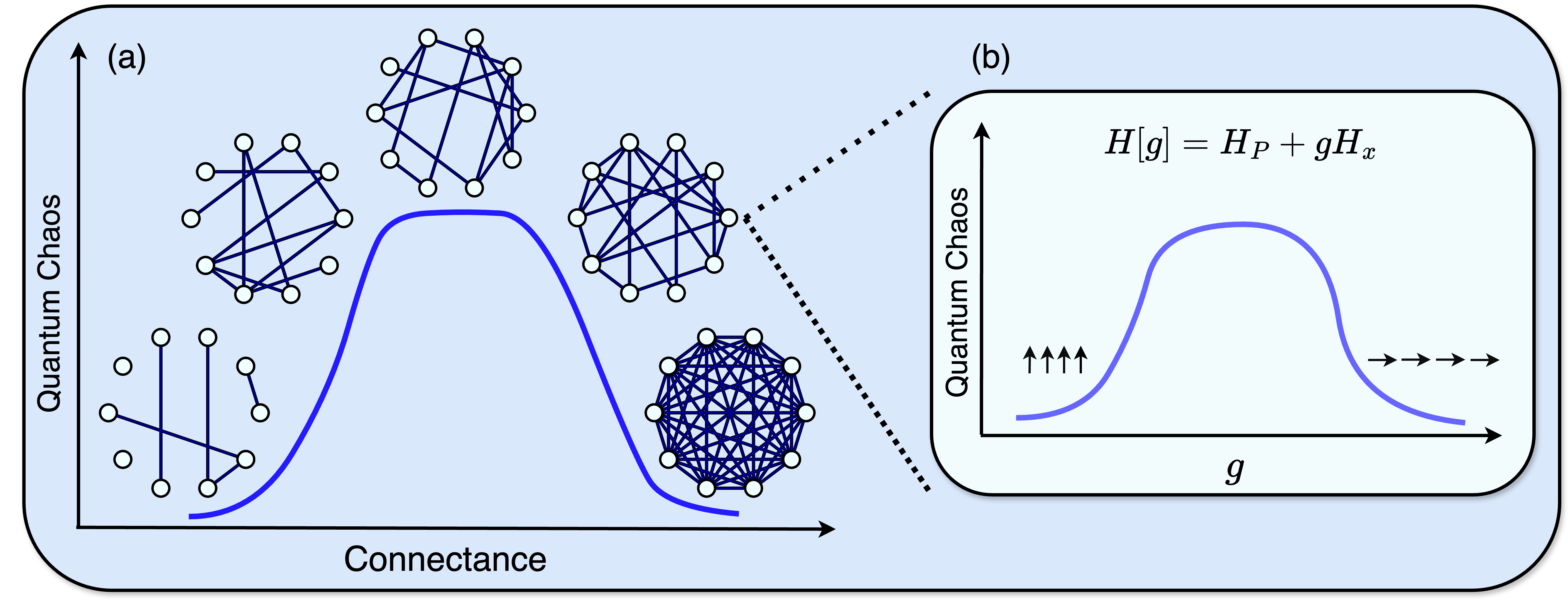
Figure 1: Schematic diagram showing an overview of the work. Each random graph $\mathcal{G}(L,M)$ corresponds to a transverse field Ising model with fixed connectance $\tilde{M}=\frac{2}{L(L-1)}M$. $(a)$ Quantum chaos is explored as a function of the connectance $\tilde{M}$ ranging from the sparsely connected regime to the LMG limit. $(b)$ Signatures of quantum chaos are inspected by varying the transverse field and the connectance.

However, establishing the boundary between quantum chaos and the MBL phase remains challenging. This comes with a numerical bottleneck as the thermodynamic limit is approached  [49, 50]. Comprehensive full-spectrum analysis has primarily been confined to Heisenberg models, with some exceptions extending to Ising spin chains [51, 52, 53, 54]. Studies of spectral characteristics have mostly incorporated the disorder in the interaction. Nonetheless, the effect of a random graph topology has been restricted to the analysis of the spin glass phase [55, 56, 57, 58] and thermal phase transitions of classical Ising models [59, 60, 61] near the ground state. Furthermore, there is a sizable literature on the eigenvalue statistics of the adjacency matrix itself [62, 63, 64, 65].

In previous works, the disorder was mostly represented by continuous random variables rather than by discrete-valued randomness. However, the latter provides a more ideal testbed for experimental realizations [66, 67, 68, 69, 70, 71]. Additionally, plenty of questions remain unanswered. For instance, when does graph randomness lead to chaotic quantum behavior? Does the exponential suppression of the long-range delocalization exist beyond the short-range perturbative regime of the transverse fields? Is the onset of quantum chaos universal?

In this work, we address these questions for an Ising model on a random graph network via the spectral form factor, the level spacing, and the level velocity statistics. In particular, we identify the regimes of the graph connectivity, where many signatures of quantum chaos disappear. Universal conditions for the onset of quantum chaos in terms of the transverse field are also investigated via large-order perturbation theory. Quantum chaotic behavior is only absent in vanishingly small regions compared to the full range of the connectivities and the transverse fields.

This work is organized as follows. In Sec. II, the structure of the spectral correlations in the computational basis is studied. In Sec. III, the spectrum is investigated numerically by a nearest-neighbor level spacing analysis with analytical methods. In Sec. IV, quantum chaos is probed via a further local measure, the level velocities. In Sec. V, the spectrum is analyzed by the spectral form factor, diagnosing quantum chaos via long-range spectral properties. Finally, we devote Sec.VI to conclusions and future directions.

II Preliminaries

This section provides details about the model and the underlying graph structure. Let us consider a general QAA Hamiltonian

$$H[g]=\frac{J}{M}\,H_{P}+\frac{g}{L}\,H_{x}\,,$$ (1)

where, $H_{x}=-\sum_{i}\,X_{i}$, $H_{P}=-\sum_{i,j}\,A_{ij}Z_{i}Z_{j}$, and $g$ is the strength of the transverse field. Here, $A_{ij}$ is the adjacency matrix with $A_{ij}=1$ for connected vertices and zero otherwise. We consider the Erdős-Rényi graphs $\mathcal{G}(L,M)$, where $(L,M)$ denotes the number of vertices and edges, as depicted in Fig. 1. Every graph configuration is sampled with probability $p=1/\begin{pmatrix}\binom{L}{2}\\ M\end{pmatrix}$. The prefactors $M$ and $L$ scale the bandwidth to the order of the energy unit $\mathcal{O}(J)$. The couplings are chosen to favor ferromagnetic ordering, $J>0$. To characterize the connectivity, we define the connectance $\tilde{M}=\frac{2}{L(L-1)}M$ [12], interpolating between the limits of disconnected graphs and the fully connected Lipkin-Meshkov-Glick model (LMG) [72]. The connectance varies in the interval $[0,1]$.

We investigate the relation between the graph randomness and the statistics of the eigenenergies of $H_{P}$. The Hamiltonian $H[g]$ can be realized as an “Anderson-like” disordered hopping model on an $L$-dimensional hypercube [73, 53],

$$H[g]=\sum_{k}\,E_{k}\,\lvert k\rangle\langle k\rvert-\frac{g}{L}\sum_{\langle k,k^{\prime}\rangle}\lvert k\rangle\langle k^{\prime}\rvert\,.$$ (2)

The disordered interactions generate the on-site energies $E_{k}$ with non-trivial correlations. The transverse field terms induce the nearest neighbor hoppings $\langle k,k^{\prime}\rangle$ via single spin flips along the edges.

In the case of random interactions, the average of the on-site energies can be shifted to zero, with the tunable energy variances characterizing the statistical properties. However, with the more constrained graph randomness, the influence of the disorder cannot be described solely by the energy variances. These variances are bounded by the finiteness of $\tilde{M}$, and the statistical properties are strongly influenced by the non-trivial structure of the mean values. Therefore, we characterize the conditions of the onset of quantum chaos by the generalized relative variances and correlations. As detailed in App. A, these quantities take the form,

$$\langle E_{k}\rangle_{\mathrm{ER}}\approx\tilde{M}\,\frac{S^{2}_{k}-L}{M}J\,,$$ (3)

$$\langle\delta E^{2}_{k}\rangle_{\mathrm{ER}}\approx 2\tilde{M}\,(1-\tilde{M})\,\frac{L^{2}}{M^{2}}J^{2}\,,$$ (4)

$$\langle\delta E_{k}\delta E_{k+r}\rangle_{\mathrm{ER}}\approx 2\tilde{M}(1-\tilde{M})\frac{L^{2}+6r(r-L)}{M^{2}}J^{2}\,.$$ (5)

Here, $S_{k}$ denotes the total spin of the $k^{\text{th}}$ spin configuration, and $\langle\delta E_{k}\delta E_{k+r}\rangle_{\mathrm{ER}}$ is the correlator of states at Hamming distance $r$ averaged over the graphs. Their most probable value varies as $S_{k}\sim\sqrt{L}$, yielding the typical scaling $\langle E_{k}\rangle_{\mathrm{ER}}\sim\tilde{M}\frac{L}{M}J$. In the thermodynamic limit, these relations become exact as the probability of a given link converges to $\tilde{M}$. The corresponding relative variances and correlations scale as

$$\frac{\sqrt{\langle\delta E^{2}_{k}\rangle_{\mathrm{ER}}}}{\langle E_{k}\rangle_{\mathrm{ER}}}\approx\sqrt{2\frac{1-\tilde{M}}{\tilde{M}}}\,,$$ (6)

$$\frac{\sqrt{\langle\delta E_{k}\delta E_{k+r}\rangle_{\mathrm{ER}}}}{\langle E_{k}\rangle_{\mathrm{ER}}}\approx\sqrt{1-\tilde{M}}\sqrt{1+6\frac{r}{L}\left(\frac{r}{L}-1\right)}\,.$$ (7)

Here, the relative strength of the correlators can be characterized by a single average value between the configurations of $k$ and $k+r$ having the same leading order behavior in $L$.

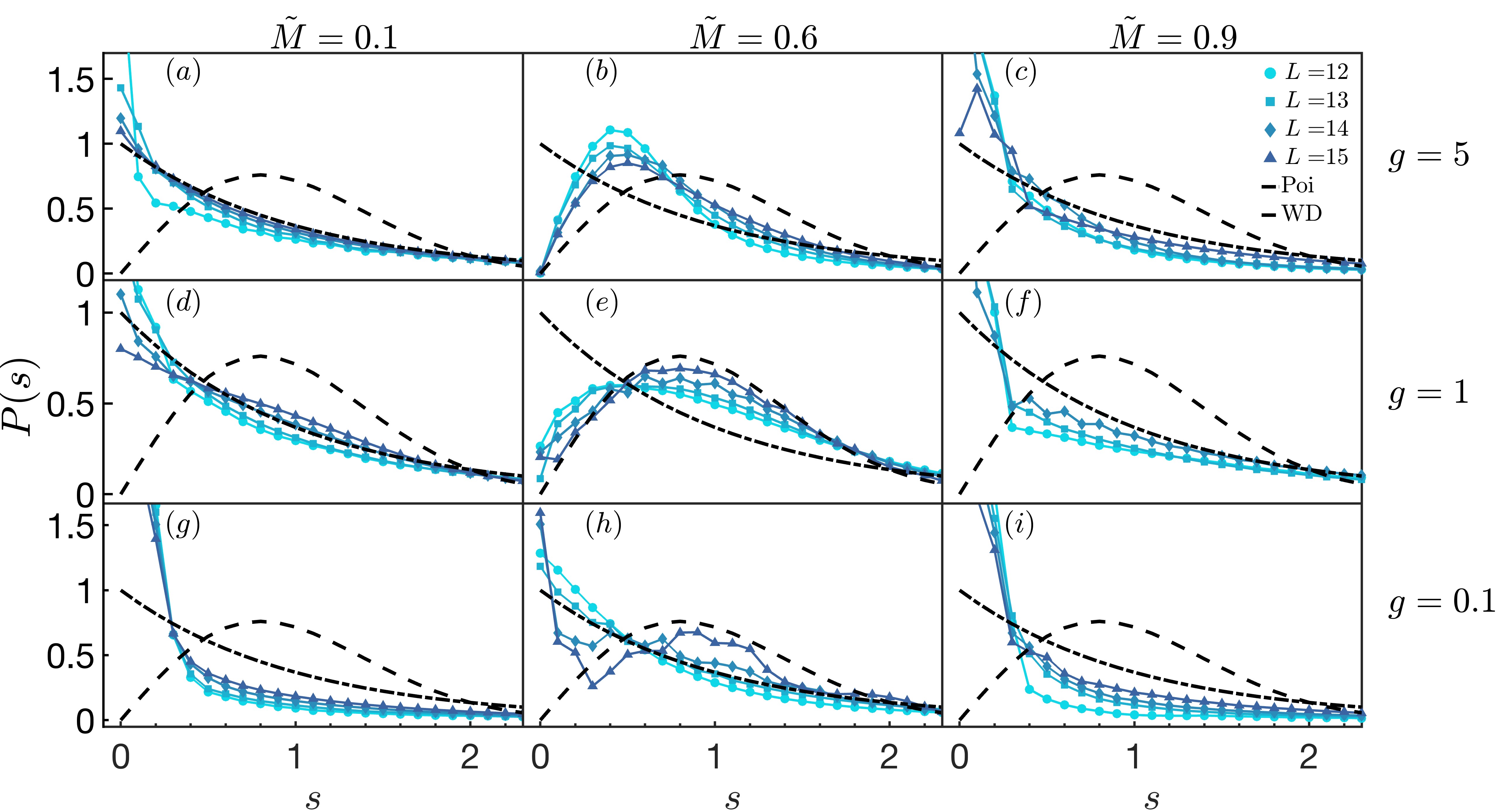
Figure 2: Nearest neighbor level spacing statistics in the perturbative $g=0.1J$, intermediate $g=J$, and strongly polarized $g=5J$ regimes, and for sparsely $\tilde{M}=0.1$, intermediate $\tilde{M}=0.6$, and densely connected $\tilde{M}=0.9$ graphs with $L=12,\,13,\,14,\,15$. The energy window $[0.3\,J,\,0.4\,J]$ was considered in the unfolded spectrum. Panels $(a)-(c)$: $g=5\,J$, displaying the perturbative breakdown of quantum chaos, recovered by the increasing system size. Restoration of quantum chaos is delayed for low and high $\tilde{M}$ in $(a)$ and $(c)$, respectively. Panels $(d)-(f)$: Similar behavior for $g=J$ with a faster restoration of quantum chaos for intermediate $\tilde{M}$. Panels $(g)-(i)$: $g=0.1\,J$, exhibiting similar features with an overall slower convergence towards the WD distribution.

III Spacing statistics analysis

In this section, local spectral analysis is performed via the statistics of the spacing between adjacent energy levels for various $g$ and $\tilde{M}$ values.

III.1 Chaotic regime of connectance and transverse field

We employ level spacing statistics at intermediate $\tilde{M}$, sufficiently outside the densely $1-\tilde{M}\sim 1/L$ and the disconnected limits $\tilde{M}\sim 1/L$. The statistics of nearest-neighbor level spacings is a prominent indicator of quantum chaotic behavior. It captures the crossover separating the chaotic and the localized regimes, as tested in various models [46, 44, 51, 52].

Quantum chaos is signaled when the level spacing statistics converges towards the Wigner-Dysnonian (WD) distribution. However, it breaks when the level statistics get concentrated around zero. An example of this is the Poissonian statistics for uncorrelated energy levels. The corresponding distribution functions are

$$P_{\mathrm{Poi}}(s)\propto e^{-s},\quad P_{\mathrm{WD}}(s)\propto s\,e^{-\frac{\pi}{4}s^{2}},$$ (8)

with the level spacing scaled to have unit average $s_{i}=\frac{E_{i+1}-E_{i}}{\langle E_{i+1}-E_{i}\rangle_{\mathrm{ER}}}$.

Yet, the spacing statistics alone does not reveal the transition towards quantum chaos. To overcome this issue, the level spacing ratio was introduced [44, 74, 54]

$$r_{i}=\frac{\min{(s_{i+1},s_{i})}}{\max{(s_{i+1},s_{i})}}\,,$$ (9)

which is robust against variations in the local density of states. It captures the emerging chaotic behavior by its average value $\langle r\rangle$, approaching $r_{\mathrm{WD}}\approx 0.523$ in the thermodynamic limit. Convergence towards either the Poissonian $r_{\mathrm{Poi}}\approx 0.386$, or a lower value signals the breakdown of quantum chaos. The level spacing ratio distributions read

$$P_{\mathrm{Poi}}(r)\propto\frac{1}{(r+1)^{2}},\quad P_{\mathrm{WD}}(r)\propto\frac{r+r^{2}}{(1+r+r^{2})^{5/2}}\,.$$ (10)

Additional spectral diagnostics via these statistics are provided in App. C.

We perform numerical simulations to investigate the onset of quantum chaos from the perturbatively small $g=0.01J$ to the fully polarized limit $g=5J$. The connectance is varied from low to high, $\tilde{M}\in[0.07,\,0.98]$. To study the spacing statistics in a spectrally resolved way, we analyze ten uniformly spaced energy windows in the unfolded spectrum. The unfolding procedure [75, 76] facilitates the characterization of the local structure of level spacing statistics. It relies on scaling out the local density of states $\rho(E)=\left\langle\sum_{i}\delta(E-E_{i})\right\rangle_{E}$, computed numerically for each graph realization. Here, the average $\langle\dots\rangle_{E}$ runs over the given energy windows. The cumulative distribution function is obtained by integrating the density, $f(E)=\int_{-\infty}^{E}\mathrm{d}E^{\prime}\,\rho(E^{\prime})$. The unfolded energies $\tilde{E}_{i}=f(E_{i})$ are then mapped by fitting a fifth-order polynomial to the cumulative distribution function.

The spectrally resolved analysis reveals the effects of the discrete-valued disorder. In particular, the total bandwidth of $H_{P}$ scales linearly with $J$ having $\frac{2J}{M}$ spacings. The number of degenerate eigenstates at $g=0$ with spins pointing opposite ways in closed loops grows exponentially with $L$. With finite $g$, the spectrum inherits this behavior to some extent. These frustrated spectral regions reside with high precision in the upper half of the spectrum, $\tilde{E}\gtrsim J/2$. We observe that the related features appear mainly at small spacing values, but do not change the overall structure of the statistics (see App. D). For these reasons, the spectral analysis is carried out in the lower half of the unfolded spectrum in the energy window of $[0.3J,\,0.4J]$. This regime is sufficiently below the frustrated upper half but close enough to the middle to test the bulk spectral properties.

As shown in Fig. 2 $(e)$ and $(h)$, for $1/L\ll\tilde{M}<1$ and $g\lesssim 4J$ the level statistics converge towards the WD distribution with increasing $L$. Meanwhile, Fig. 2 $(g)-(i)$ show that decreasing the $g$, increases the deviations, resulting in a slower convergence. This behavior can be captured using first-order perturbation theory at $g=0$. The overlap is computed between two non-degenerate eigenstates $\lvert k_{1}\rangle,\,\lvert k_{2}\rangle$, separated by unit Hamming distance around the middle of the energy spectrum,

$$T_{k_{1},k_{2}}\approx\frac{g}{L}\frac{1}{\Delta E_{12}},$$ (11)

where $\Delta E_{12}\sim\frac{\sqrt{L}}{M}$ is the typical scale of the energy difference (see App. A). Requiring that $T_{k_{1},k_{2}}\sim\mathcal{O}(1)$ in the thermodynamic limit sets the threshold of the transverse field $g\gtrsim L^{-1/2}J$. Below this scale, the energy contributions are smaller than the mean level spacing between non-degenerate eigenstates differing by one spin-flip. The transverse field provides only small corrections, implying trivially localized behavior. Thus, the spacing statistics gets concentrated around zero more than the Poissonian distribution with a Shnirelman peak [77, 78], as displayed in Fig. 2 $(g)-(i)$. Similar behavior was reported in Heisenberg models with strongly correlated random longitudinal fields [79, 80]. However, with increasing $L$, the spectrum escapes this perturbative regime at fixed $g$ values and develops chaotic behavior, as displayed by Fig. 2 and Fig. 3 $(h)$. To understand the non-trivial breakdown of quantum chaos, we examine the condition for long-range delocalization between eigenstates separated by $\sqrt{L}$ Hamming distances.

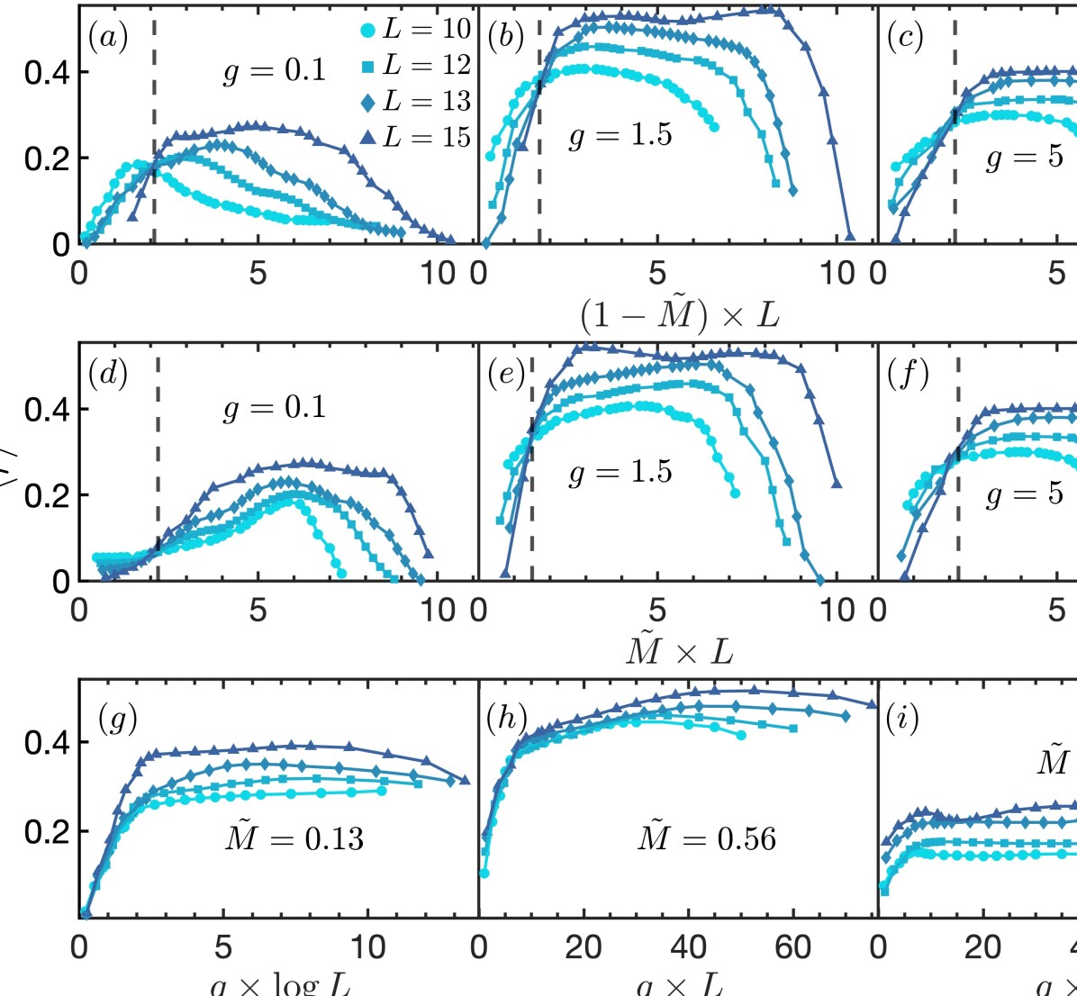
Figure 3: Level spacing ratio as a function of $\tilde{M}$ and $g$ for $L=10,12,13,15$ in the energy window $[0.3\,J,\,0.4\,J]$ of the unfolded spectrum. Panels $(a)-(c)$: Level spacing ratio as a function of $(1-\tilde{M})\times L$ for $g=0.1J,\,1.5J,\,5J$, exhibiting the transition to the fully connected limit around $(1-\tilde{M})\times L\approx 2$. Panels $(d)-(f)$: Same $g$ values predicting the breakdown of quantum chaos around the disconnected limit at $\tilde{M}\times L\approx 1.8$. Panels $(g)-(i)$: Level spacing ratios as a function of the rescaled $g$ for low, intermediate, and high $\tilde{M}$ values.

As shown in App. B, perturbative corrections of order $n\sim\sqrt{L}$ order in the forward scattering approximation [81, 53] result in an amplitude,

$$\begin{split}&T_{k_{1},k_{2}}\propto\left(\frac{g}{L}\right)^{n}\sum_{m_{1},m_{2},\cdots,m_{n-1}}(H_{x})_{k_{1},m_{1}}\cdots(H_{x})_{k_{1},k_{2}}\\ &\times\left(\Delta E_{k_{1},k_{2}}\prod_{i=1}^{n-1}\Delta E_{k_{1},m_{i}}\right)^{-1}\sim\left(\frac{gL}{J}\right)^{n},\end{split}$$ (12)

posing the lower boundary $g\gtrsim L^{-1}J$. For these $g$ values, exponential suppression of eigenstate delocalization breaks down and quantum chaos sets in as a universal function of $g\times L$. This is verified by the scaling collapse of the $\langle r\rangle$ values in Fig. 3 $(h)$. Furthermore, the dominance of long-range spreading of the eigenstates implies that no mobility edge exists, in agreement with Fig. 3 $(g)-(i)$.

By contrast, in the single-particle case [82, 83, 84], the critical values of the hopping amplitudes are of the same order as the mean level spacing. The present analysis predicts similar behavior as approximate methods in Refs. [32, 85]. The analysis of the $\langle r\rangle$ values for $g=0.1\,J$ and $g=1.5\,J$, exhibits the same behavior. As shown in Fig. 3 $(a),\,(b),\,(d)$ and $(e)$, convergence for intermediate $\tilde{M}$ is observed towards the chaotic value $r_{\mathrm{WD}}\approx 0.52$. In agreement with the results of the spacing statistics, convergence is the fastest for intermediate $g$ values.

Figure 4: Level velocity distributions for $L=14$ scaled to unit variance, compared with a standard Gaussian distribution. The figure shows results for $(a)$ $\tilde{M}=0.18$, $(b)$ $\tilde{M}=0.49$, and $(c)$ $\tilde{M}=0.71$. The breakdown of the Gaussian curve is observed as the transverse field $g$ increases. This breakdown happens for smaller $g$ values as $\tilde{M}$ increases.

III.2 Sparsely and densely connected graphs and strongly polarized limit

Next, we turn to the cases of low connectance with a growing number of disconnected subnetworks, $\tilde{M}\lesssim 2/L$, and the LMG limit with $1-\tilde{M}\gtrsim 2/L$.

The ER graph splits up to disconnected subnetworks of size $\sim\log L$ [19, 20] when the connectivity reaches the order of the number of vertices. It simplifies to $\tilde{M}=\frac{1}{L}$ in the thermodynamic limit. The agreement with the WD statistics naturally breaks down due to these graph-theoretical features. The energy spectrum splits up to the sum of the $\sim L/\log L$ completely uncorrelated spectra with $\sim 2^{\log L}$ energy levels. As $L$ grows, the number and sizes of the subnetworks increase. This leads to a larger chance of an arbitrary degree of degeneracy. This is in contrast with the Poissonian case of independent identical levels. Thus, the corresponding spacing statistics goes beyond the Poissonian for small spacings.

However, the disconnected regime survives only when the rescaled connectance is kept constant, $\tilde{M}\,L\lesssim 1$. For fixed $\tilde{M}$, the system inherently escapes this regime and restores quantum chaos. The perturbative argument of the onset of chaos in Eq. (12) naturally carries on to the disconnected subnetworks. This implies that the universal scale of $g$ is governed by the small subgraph sizes separately. As demonstrated in Fig. 3 $(g)$, this leads to the scaling collapse as a function of $g\times\log L$. The convergence towards the WD distribution for fixed $\tilde{M}$ are displayed in Fig. 2 $(a),\,(d)$ and $(g)$.

Remarkably, the level spacing ratio captures this connected-disconnected transition point. As shown in Fig. 3 $(d)-(f)$, at fixed $g$ values, the corresponding ratio curves cross each other at approximately the same value of the rescaled connectance, $\tilde{M}L\approx 1.8$. This slight deviation from the theoretical value is the consequence of finite-size effects, which are especially relevant in the disconnected subgraphs. Additionally, the transition point shifts to higher values for limiting $g$ due to additional localization effects. These findings are demonstrated in Fig. 3 $(d)-(f)$ for small, intermediate, and large $g$ values.

Turning to the opposite limit, the scale $1-\tilde{M}\gtrsim 2/L$ naturally leads to the vanishing of the relative variances and correlations according to Eq. (6),

$$\frac{\sqrt{\langle\delta E^{2}_{k}\rangle_{\mathrm{ER}}}}{\langle E_{k}\rangle_{\mathrm{ER}}}\sim L^{-1/2}\,,$$ (13)

$$\frac{\sqrt{\langle\delta E_{k}\delta E_{k+r}\rangle_{\mathrm{ER}}}}{\langle E_{k}\rangle_{\mathrm{ER}}}\sim L^{-1/2}\sqrt{1+6\frac{r}{L}\left(\frac{r}{L}-1\right)}\,.$$ (14)

This implies that with increasing $L$, on-site energy distributions get concentrated around the average $\langle E_{k}\rangle_{\mathrm{ER}}=\tilde{M}\frac{S^{2}_{k}-L}{M}$. Thus, the spectrum becomes identical to that of the LMG model up to a $\mathcal{O}(1)$ factor with a relative error of

$$\frac{E_{k}-E^{\mathrm{LMG}}_{k}}{E^{\mathrm{LMG}}_{k}}\sim\mathcal{O}(L^{{-1/2}})\,.$$ (15)

Here, $E^{\mathrm{LMG}}_{k}=\frac{S^{2}_{k}-L}{M}$ denotes the energy of the LMG model at $g=0$. This error originates from the on-site variances rather than from the $\tilde{M}$ prefactor. Involving $H_{x}$ to the Hamiltonian will result in the same relative error compared to the transverse field LMG model [86].

Close to the fully connected limit, quantum chaos breaks around the complementary scale of the disconnected limit, $1-\tilde{M}\approx 2/L$. The transition also becomes sharp, as captured by the level spacing ratios. In Fig. 3 $(a),\,(b)$ a transition point as a function of $(1-\tilde{M})\times L$ is displayed. The crossover sets in at slightly larger values than $1-\tilde{M}\gtrsim 2/L$ for limiting $g$ values. Furthermore, the level statistics converge towards the WD distributions with $L$, as shown in Fig. 2 $(c),(f)$, and $(i)$. These results show the main difference between fixing $\tilde{M}$ or $(1-\tilde{M})\times L$. The former leads to a convergence towards the regime of intermediate $\tilde{M}$ and quantum chaos. In the latter case, the system stays near the LMG limit with vanishing on-site fluctuations upon increasing $L$. This explains well the decreasing behavior of the $\langle r\rangle$ values, as demonstrated Fig. 3 $(a)-(c)$.

Figure 5: Level velocity distributions for low to high connectances $\tilde{M}=[0.18,0.73]$. The figure shows results for $(a)$ $L=14,g=0.4\,J$, and $(b)$ $L=15,g=J$. For the larger $g$ value, the velocity statistics break down earlier with increasing $\tilde{M}$.

III.3 Strongly polarized limit

Finally, the strongly polarized limit $g\gg J$ is discussed, which provides similar thresholds for the breakdown of the quantum chaotic behavior. Large $g$ values lead to localization in the $X$ polarized basis. Due to the degeneracies in the $X$ basis, the spacing statistics clusters around zero more pronouncedly than the Poissonian distribution. Near the LMG limit, the rescaled transition connectance $(1-\tilde{M})\times L$ increases with $g$ entering the intermediate regime. For fixed $\tilde{M}$, the increasing $L$ restores quantum chaos, as observed in Fig. 2 $(c)$ and Fig. 3 $(i)$. In the connected $2/L\ll\tilde{M}<1-2/L$, and disconnected $\tilde{M}\lesssim 2/L$ regimes, distinct scalings are found for the onset of quantum chaos. For intermediate $\tilde{M}$, first order perturbative approximation of the overlap of two $X$ polarized eigenstates, $\lvert x_{1}\rangle,\,\lvert x_{2}\rangle$ scales as

$$T_{x_{1},x_{2}}\approx\frac{LJ}{Mg}\sim\frac{J}{Lg}\,.$$ (16)

Here, the two eigenstates are separated by two spin-flips around the middle of the spectrum, which fixes the threshold as $g\lesssim L^{-1}J$. This threshold accounts for the short-range suppression of the delocalization in the $X$ basis. By contrast, the onset of quantum chaos near the strongly polarized limit is better encapsulated by long-range delocalization. Employing again the forward scattering approximation of order $n\sim\sqrt{L}$, we obtain

$$\begin{split}&T_{x_{1},x_{2}}\propto\sum_{m_{1},\cdots,m_{n-1}}(H_{P})_{x_{1},m_{1}}\cdots(H_{P})_{m_{n-1},x_{2}}\\ &\times M^{-n}\left(\Delta E_{x_{1},x_{2}}\prod_{i=1}^{n-1}\Delta E_{x_{1},m_{i}}\right)^{-1}\sim\left(\frac{\sqrt{L}J}{g}\right)^{n},\end{split}$$ (17)

leading to the threshold of $g\lesssim L^{1/2}J$ (see App. B). Therefore, strong transverse field terms cannot challenge quantum chaos beyond suppressing short-range hybridization. Increasing $L$ facilitates the restoration of quantum chaos. The convergence of the level statistics and the spacing ratios are presented in Fig. 2 $(a)-(c)$ and Fig. 3 $(c),\,(f)$. This convergence slows down near the disconnected and fully connected regimes. The whole procedure can be repeated in the disconnected regime by replacing $L$ with $\log L$. The uncorrelated subnetworks are separately governed by the strong transverse fields. This implies that the threshold scales with the subnetwork sizes, $g\sim\sqrt{\log L}J$.

IV Level velocity analysis

This section addresses the chaotic signatures of the spectrum from the point of view of energy level dynamics [87, 88, 35]. The parametric variations of energy levels of a Hamiltonian $H[g]$ capture non-equilibrium phenomena induced by external driving potentials in disordered systems. The corresponding derivative of the energy levels is referred to as “level velocity” $v_{n}=\frac{\mathrm{d}E_{n}}{\mathrm{d}g}$. This quantity effectively measures the sensitivity of the spectrum against external perturbations. Prominent examples are the fluctuations of the microscopical conductance in the presence of time-dependent magnetic fields [89, 90]. Further research has focused on level dynamics in disorder Heisenberg models and one-dimensional quantum systems [91, 92, 93]. Universal velocity correlations were revealed in disordered hopping models with changing boundaries. Analytical velocity statistics were derived in the localized phase of driven Anderson models [94, 95, 96, 97].

Figure 6: Level velocity statistics scaled to unit variance compared to standard Gaussian distribution. The figure shows results for $(a)$ $g=0.5\,J,\tilde{M}=0.49$, $(b)$ $g=0.75\,J,\tilde{M}=0.4$, $(c)$ $g=J,\tilde{M}=0.24$, for $L=10,11,13,15$. Increasing $L$ leads to the breakdown of the Gaussian shape. This is observed for $L=13,15$ whereas $L=10,11$ approximately follows the Gaussian curve. Furthermore, deviations appear earlier for increasing $g$ and $\tilde{M}$.

Similar to spacing statistics, level velocity

$$v_{n}=\frac{\mathrm{d}E_{n}}{\mathrm{d}g}=\frac{1}{L}\bra{n}{H}_{x}\ket{n},$$ (18)

also provides a local characterization of the spectral properties. Here, $\ket{n}$ refers to the eigenstate of $H[g]$ in Eq. (1). To this end, we probe chaotic signatures via $v_{n}$ as a function of $g$ and $\tilde{M}$.

The level velocity provides valuable insights into the statistical properties of both the eigenvalues and eigenstates. To capture the local spectral properties, the unfolding method is applied similarly to level spacing,

$$v_{n}\rightarrow\tilde{v}_{n}=\frac{d\tilde{E}_{n}}{dg}=\rho(E_{n})v_{n},$$ (19)

where $\tilde{v}_{n}$ represents the unfolded level velocities. The eigenstates of $H[g]$ can be expanded as

$$v_{n}=\frac{1}{L}\bra{n}{H}_{x}\ket{n}=\frac{1}{L}\sum_{k,l}C_{l}^{*}C_{k}\bra{l}{H}_{x}\ket{k},$$ (20)

where $\ket{k},\ket{l}$ are the eigenstates of $H_{P}$, with amplitudes $C_{k}$, $C_{l}$. The non-zero terms in Eq. (20) occur when $\ket{k}$ and $\ket{l}$ differ by only one spin, leading to

$$v_{n}=\frac{1}{L}\sum_{k,l}C_{l}^{*}C_{k}\delta(\Delta S_{kl}-1),$$ (21)

where $\Delta S_{kl}=\sum_{i}|\sigma^{(k)}_{i}-\sigma^{(l)}_{i}|$ and $\sigma^{(k)}_{i}=\pm 1/2$ denotes the $i^{\text{th}}$ spin $Z$ value of the $k^{\text{th}}$ spin configuration. Based on the level spacing analysis, eigenstates are captured by RMT up to high precision. This leads to approximately independent and extended amplitudes $C_{k},\,C_{l}\sim\frac{1}{\sqrt{2^{L}}}$. Thus, Eq. (21) leads to Gaussian velocity statistics in quantum chaotic spectral regions, which is in agreement with previous findings  [98, 99]. However, its deviation from the Gaussian shape does not necessarily capture the integrable regimes. In contrast to the spacing statistics, $v_{n}$ is governed by short-ranged eigenstate delocalization for small $g$. In Eq. (21), $C_{k},\,C_{l}$ spread uniformly over the threshold $g\gtrsim L^{-1/2}$.

The breakdown of the level velocity statistics can be understood via first-order perturbation theory. For small $g$ values, $H_{x}$ can be treated as a perturbation to $H_{P}$. In this limit (see App. E)

$$v_{n}\sim g\sqrt{\tilde{M}}.$$ (22)

Tentatively, the breakdown is identified when this result matches the velocity scale in the strongly polarized regime, $g\gg J$. In this limit, Eq. (18) is governed by the eigenstates of $H_{x}$ in leading order around the middle of the spectrum yielding (see App. E),

$$v_{n}\sim\frac{1}{\sqrt{L}}\,.$$ (23)

Comparing Eq. (22) and Eq. (23) leads to the threshold scale

$$g\propto\frac{1}{\sqrt{\tilde{M}L}},$$ (24)

where $v_{n}$ breaks down. It further validates the first-order perturbation approach since, for large $L$, low-order perturbation corrections converge with the breakdown scale.

The velocity statistics break down near the perturbatively small and strongly polarized $g$ limits at fixed $\tilde{M}$ and $L$, as shown in Fig. 4. The dependence on the connectance exhibits different behavior in the disconnected limit $\tilde{M}\sim 1/L$, as the Gaussian shape persists with reasonably increased variances. In this regime, velocity statistics accurately capture the remaining chaotic signatures of the individual subnetworks. Gaussian velocity statistics survive separately in these disconnected parts, which sum up as independent random variables. This results in a final normal distribution in line with the central limit theorem. However, the densely connected regime exhibits the same behavior as in the preceding section, where Gaussian shape and quantum chaos break down. These results are presented in Fig. 5.

Furthermore, in the disconnected regime, the upper threshold of $g$ also increases in contrast to the spacing analysis. This property is well explained by the scaling in Eq. (24) as the crossover connectance $\tilde{M}\sim 1/L$ implies a size-independent threshold of $g$. Close to the fully connected limit, quantum chaos survives only in a narrower window of $g$, as similarly revealed by the spacing analysis.

In contrast to the level spacing statistics, increasing $L$ leads to the breakdown of the chaotic character. Near the strongly polarized limit, considering $H_{P}$ as a small perturbation, the velocity reads

$$v_{n}=\frac{1}{L}\sum_{x_{l},x_{k}}\,C^{*}_{x_{l}}C_{x_{k}}\left\langle x_{l}\left\lvert H_{x}\right\rvert x_{k}\right\rangle=\frac{1}{L}\sum_{x_{k}}\,\lvert C_{x_{k}}\rvert^{2}\,,$$ (25)

with $\lvert x_{l}\rangle,\lvert x_{k}\rangle$ denoting the eigenstates of $H_{x}$. Here, the velocity statistics are governed by the amplitudes of the $X$ polarized eigenstates. The spreading of these eigenstates becomes strong enough when $g$ is sufficiently below the long-range delocalization threshold. The $C_{x_{k}}$ amplitudes delocalize in the $X$ basis satisfying the conditions of Gaussian velocity statistics at the scale $g\sim L^{-1/2}$. The system size breakdown is illustrated in Fig. 6. For smaller sizes $L=10,11$, the distribution still follows precisely the Gaussian shape, whereas the statistics for higher ones with $L=13,15$ show clear deviations.

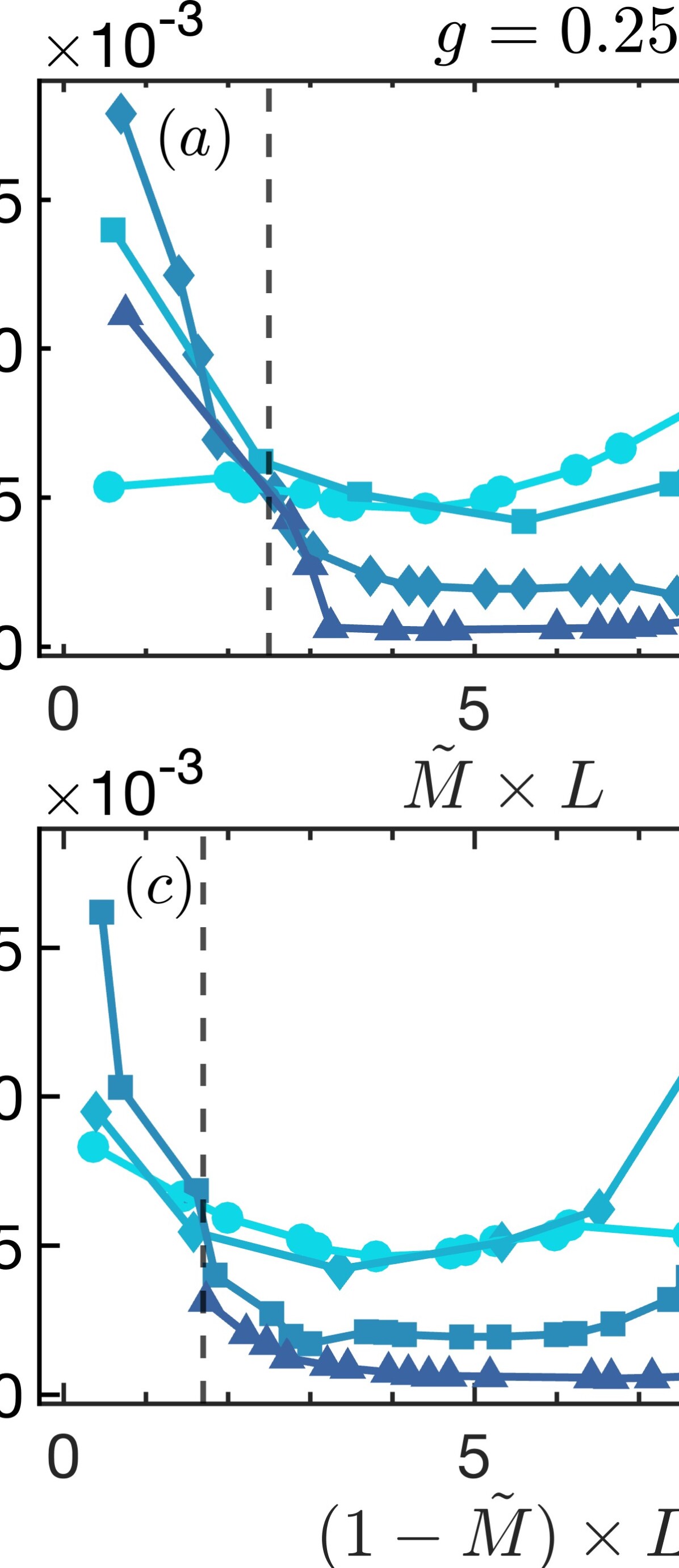
Figure 7: Rescaled level velocity variances for $g\lesssim 1.25\,J$ values where the Gaussian shape persists. Panels $(a)$ and $(b)$: Transition point around the disconnected regime as a function at $\tilde{M}\times L\approx 1.8$ for $g=0.25\,J,\,0.4\,J$. Panels $(c)$ and $(d)$: Transition towards the LMG limit at $(1-\tilde{M})\times L\approx 1.6$ for $g=0.25\,J,\,0.4\,J$.

The variance of the level velocities is investigated both in the connected and the disconnected regimes around the middle of the spectrum. Using Eq. (21) the approximate RMT description of the eigenstates, the variance reads as

$$\left\langle\delta v^{2}\right\rangle\sim\frac{1}{L}\sum_{k,l}\left\langle(C_{l}^{*}C_{k})^{2}\right\rangle\delta(\Delta S_{kl}-1).$$ (26)

Approximating $C_{k},\,C_{l}\sim 1/\sqrt{2^{L}}$ Eq. (26) becomes

$$\left\langle\delta v^{2}\right\rangle\sim\frac{1}{L}\sum_{k,l}\frac{1}{2^{2L}}\delta(\Delta S_{kl}-1).$$ (27)

However, there are a total of $2^{L}L$ possible ways to obtain non-zero delta functions. Hence, $\left\langle\delta v^{2}\right\rangle\sim\frac{2^{L}L}{L}\frac{1}{2^{2L}}\sim\frac{1}{2^{L}}$, in the chaotic region. This analysis predicts a fast decrease in $\left\langle\delta v^{2}\right\rangle$ with respect to the system size $L$. The corresponding level velocity statistics are depicted in App. E.

In the sparsely connected regime, $\langle\delta v^{2}\rangle$ exhibits a different scaling. Although the chaotic behavior of the velocities survives in the disconnected regime, $\langle\delta v^{2}\rangle$ still captures the corresponding transition point. The variance exhibits a sudden growth around $\tilde{M}\approx 2/L$ due to the independence of the chaotic subnetworks. In particular, the level velocities of the subnetworks add up as independent Gaussian random variables, eventually leading to a larger system size scale of $\langle\delta v^{2}\rangle$,

$$\begin{split}\left\langle\delta v^{2}\right\rangle&\sim\frac{1}{L}\sum_{\mathrm{subgraphs}}\sum_{k,l}\left({\frac{1}{{2^{\log L}}}}\right)^{2}\delta(\Delta S_{kl}-1)\\ &\sim\frac{1}{L}\sum_{\mathrm{subgraphs}}\frac{1}{2^{2\log L}}2^{\log L}\log L\\ &\sim\frac{1}{L}\frac{\log L}{2^{\log L}}\frac{L}{\log L}=L^{-\log 2}.\end{split}$$ (28)

The first summation is performed over the $L/\log L$ disconnected subnetworks. This leads to a decrease in $\langle\delta v^{2}\rangle$ with increasing $L$ in the thermodynamic limit. As shown in Fig. 7 $(a)$ and $(b)$, $\langle\delta v^{2}\rangle\times L$ captures the disconnected transition point around $\tilde{M}\approx 1.8/L$. Remarkably, the LMG limit is also captured by $\langle\delta v^{2}\rangle\times L$ as a function of the rescaled connectance $(1-\tilde{M})\times L$, as demonstrated in Fig. 7 $(d)$ and $(e)$.

V Spectral form factor

In this section, quantum chaotic signatures are tested by the spectral form factor (SFF) analysis. In contrast to the local analysis, SFF probes both short and long-range spectral correlations. In this approach, one accesses the two-point correlation function via its Fourier transform. It is controlled by a continuous time parameter $t$,

$$S_{t}=\frac{1}{N^{2}_{\mathrm{av}}}\left\langle\left\lvert\sum_{i=1}^{N_{\mathrm{av}}}e^{-i2\pi tE_{i}}\right\rvert^{2}\right\rangle_{\mathrm{ER}}\,,$$ (29)

where $N_{\mathrm{av}}$ is the number of the investigated eigenvalues. The SFF studies range from comparing it to local spectral statistics [100, 101, 102, 103, 104], to quantum chaos and MBL [75, 105]. Spectral properties in systems with classically chaotic counterparts [30, 106, 107, 108, 36] and the quantum decay rate via the survival probability [109, 110, 111, 112] were also investigated.

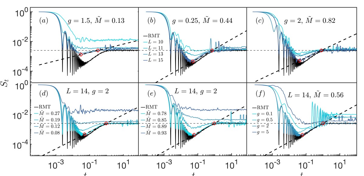
Figure 8: Spectral form factors for different $g,\,\tilde{M}$ and $L$ values for $N_{\mathrm{av}}=400$ energy levels around the middle of the spectrum. The linear ramp is indicated between $t_{\mathrm{Th}}$ and $t_{H}$ for the comparison with the RMT result. Panels $(a)-(c)$ exhibit the breakdown of the chaotic SFF for different $(\tilde{M},g)$ pairs with varying $L$. Panels $(d)$ and $(e)$ show similar breakdown for $L=14$ with varying $\tilde{M}$ for $g=2\,J$, whereby panel $(f)$ shows similar features varying $g$, for $\tilde{M}=0.56$.

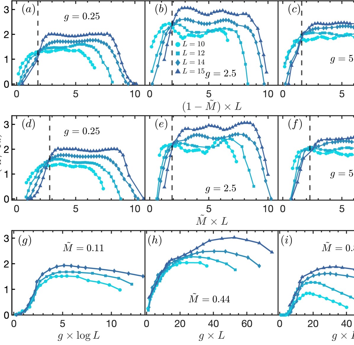
Figure 9: Logarithmic ratios of $t_{H}$and $t_{\mathrm{Th}}$ characterizing the correlation hole with varying $\tilde{M}$ and $g$ values for $L=10,\,12,\,14,\,15$. Panels $(a)-(c)$: Transition to the transverse field LMG limit as a function of $(1-\tilde{M})\times L$ for $g=0.25\,J,\,2.5\,J,\,5\,J$. Panels $(d)-(f)$: Transition to the disconnected limit as a function of $\tilde{M}\times L$ for the same $g$ values. The vertical dashed line indicates the transition point in both cases. Panels $(g)-(i)$: $g_{H}$ as a function of the rescaled $g$, for $\tilde{M}=0.11,\,0.44,\,0.89$ exhibiting the universal onset of quantum chaos.

For short time scales compared to the mean level spacing, $t\ll\delta\epsilon^{-1}$ spectral correlations at large separations dominate, resulting in a polynomial decaying shape. In terms of the survival probability, initial short-time behavior corresponds to large energy scales, allowing for level-to-level transitions regardless of the spectral distance. This regime is governed by long-range level repulsion, inducing a characteristic oscillatory behavior for a chaotic spectrum. This “dip” regime decays as $t^{-3}$ for chaotic and as $t^{-2}$ for the Poissonian regimes.

At intermediate time scales, the SFF exhibits a correlation hole, which is one of the most prominent signatures of quantum chaos governed by short-ranged level repulsion. The correlation hole sets the many-body Thouless time $t_{\mathrm{Th}}$ [112]. It characterizes the time scale required to explore the Hilbert space in line with the ergodic hypothesis. For $t>t_{\mathrm{Th}}$, quantum chaotic systems exhibit a linear ramp starting from the minimum of the correlation hole and saturating at $S_{t\rightarrow\infty}=\frac{1}{N_{\mathrm{av}}}$. This sets the relaxation or Heisenberg time $t_{H}$. It naturally captures the inverse of the mean level spacing $\delta\epsilon$ below which all level-to-level transitions are suppressed. In the Poissonian regime, the correlation hole does not emerge, and the short-time power-law decay immediately turns into a plateau. The absence of the correlation hole is equivalent to the breakdown of ETH and also provides a frequent signal of the emerging MBL phase [75, 105, 113].

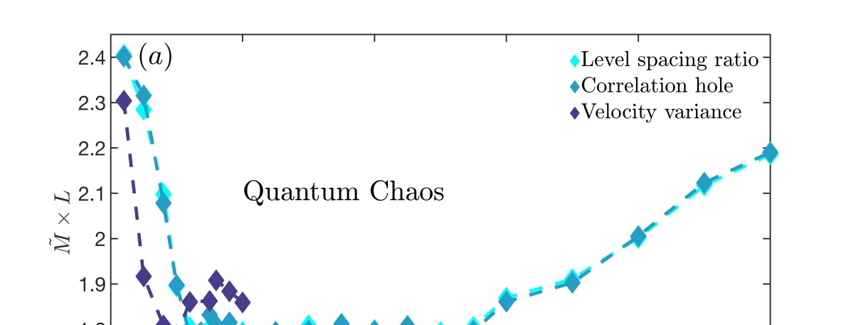
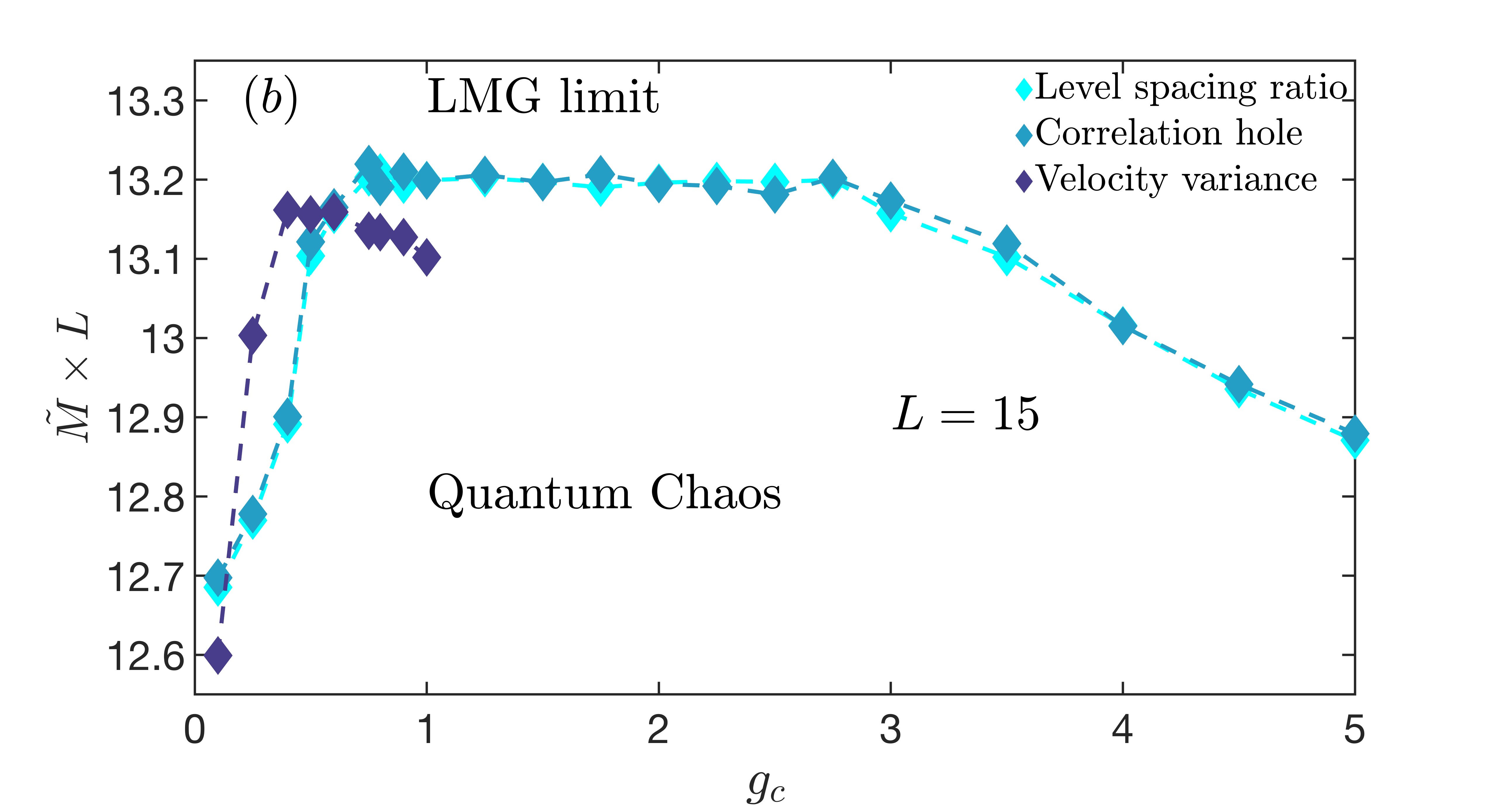
Figure 10: Phase diagram in the parameter space $(\tilde{M},g)$, separating the quantum chaotic regions via the local and global measures of the level spacing ratio, the velocity variance, and the correlation hole. Panel $(a)$ shows the transition to the regime of disconnected networks as a function of the rescaled connectance $\tilde{M}\times L$. Panel $(b)$ shows the transition to the LMG integrable limit as a function of the rescaled connectance for $L=15$.

Beyond $t_{H}$, coherent oscillations cancel out every contribution to the plateau $1/N_{\mathrm{av}}$. This changes completely for frustrated energy levels with exact or quasi-degeneracies. In particular, adjacent levels approaching much closer than $\delta\epsilon$ give rise to strong oscillations beyond $t_{H}$. Exact degenerate states with zero exponents persist at arbitrary long-time scales, leading to a constant shift of the plateau. While these effects break down the local spectral analysis, the correlation hole survives [114]. This allows for the identification of quantum chaos as demonstrated in Fig. 8 $(b),(e),(f)$.

The relative range of the correlation hole provides an efficient measure of the degree of chaoticity, captured by the logarithmic ratio of $t_{H}$ and $t_{\mathrm{Th}}$ [75] given by

$$g_{H}=\ln(t_{H}/t_{\mathrm{Th}})\,.$$ (30)

It compares the relative size of the correlation hole to the corresponding RMT model with $N_{\mathrm{av}}$ investigated levels.

For chaotic spectra, $g_{H}$ diverges with the number of levels, while for localized systems, it converges to zero in the thermodynamic limit. To focus on the width of the correlation hole, all SFF curves were normalized as $S_{t=0}=1$. The spectrum was unfolded to the energy range $[0,2^{L}\,J]$. This choice sets $t_{H}\approx 1/J$ around the middle of the spectrum. The minimum position of the correlation hole identifies $t_{\mathrm{Th}}$.

To this end, quantum chaotic behavior was probed for the same data as via the local measures around the middle of the spectrum. As shown in Fig. 8 $(a)-(c)$, the short and the long-time behavior of the SFFs converges with increasing $L$ towards the corresponding RMT curve. The dependence of the SFF curves on $\tilde{M}$ is also in good agreement with the predictions of the local analysis. Increasing $L$ aids the system in escaping the limiting regimes of $g$ and $\tilde{M}$. The SFF exhibits a crossover to a Poissonian-like shape for low and high $\tilde{M}$. For low $\tilde{M}$, this happens on smaller time scales due to the smaller system sizes of the disconnected subnetworks, as demonstrated in Fig. 8 $(d)$ and $(e)$. In this regime, the degeneracies appearing in the peaks of the level statistics around zero induce a constant shift of the plateau. Similar to the level spacing ratios, $g_{H}\rightarrow 0$ values capture the crossovers to the fully connected and the disconnected limits. These regimes are separated approximately at $\tilde{M}\approx\frac{1.8}{L}$ and $1-\tilde{M}\approx\frac{2}{L}$ for intermediate $g$. Moreover, these transition points get slightly shifted in the extreme transverse field regimes, as demonstrated in Fig. 9 $(a)-(f)$. The localization effects destroy the correlation hole for small and large $g$, as shown in Fig. 8 $(f)$. Additional oscillations appear beyond the ramp owing to the original degeneracies. In both limits, increasing $L$ restores the chaotic behavior and helps the system to develop a correlation hole. The logarithmic ratio $g_{H}$ follows approximately a universal curve as a function of $g\times\log L$ in the disconnected and $g\times L$ in the connected regimes. These findings are presented in Fig. 9 $(g)-(i)$.

The local and SFF measures allow us to spot the transition points in the space of $(\tilde{M},g)$ as observed in Fig. 10. For intermediate $g$, the scales $\tilde{M}\sim 2/L$ and $(1-\tilde{M})\sim 2/L$ separate the chaotic regimes from the disconnected and fully connected limits, respectively. These values become slightly larger when approaching the polarized and perturbative regimes. Here, $\left\langle\delta v^{2}\right\rangle$ remains a proper measure for $g\lesssim 1$. Integrability is restored in the fully connected regime by reaching the transverse field LMG limit. Poissonian-like behavior naturally arises in the disconnected limit due to the independent subgraphs. However, the spectral nature of the small subnetworks preserves their chaotic behavior.

VI Conclusions

We have reported that random Ising networks exhibit quantum chaos, originating from the underlying Erdős-Rényi graph topology. We investigated the level spacing statistics, the level velocity distributions, and the spectral form factor.

The spin Hamiltonian with ferromagnetic interactions and connectivity given by the Erdős-Rényi random graph was mapped to a hopping model on an $L$ dimensional hypercube. The ratio of the on-site energy correlations and the averages allowed for the analytical treatment of the onset of quantum chaos as a function of the connectance and the transverse field. The level spacing statistics captures the transitions in the limiting regimes of the connectance. In the disconnected regime, the Wigner-Dyson spectral statistics breaks down due to the independence of the disconnected parts. Increasing the connectance washes out randomness and develops integrable behavior as the fully connected limit is approached. However, these disconnected and LMG limits only survive for connectances converging to zero and unity, respectively, in the thermodynamic limit. As for the transverse field dependence, a universal system size scale was computed by large-order perturbation theory and verified numerically. This approach captures the onset of quantum chaos via the condition of long-range delocalization.

Supplementing the level spacing analysis, the level velocity statistics was also employed as a local spectral diagnostics. In particular, Gaussian velocity statistics is found in the chaotic regime, which survives in the disconnected subnetworks as well. In contrast to the spacing distributions, level velocities are governed by short-range delocalization, capturing different regimes of quantum chaos. Remarkably, the velocity variance provided a new measure to capture the crossovers to both the disconnected and the fully connected regimes.

Finally, we investigated level correlations via the spectral form factor at arbitrary spectral distances. The correlation hole provides an efficient quantum chaotic indicator in spectral regimes where level spacing and velocity statistics exhibit slight deviations. The spectral form factor curves and the correlation hole exhibit similar conditions for the breakdown of quantum chaos. In particular, the correlation hole vanishes in the disconnected and the fully connected limits. The former originates from the independence of the subnetworks, not accounting for the remaining chaotic signatures. The latter captures the LMG limit, similar to that observed in the spacing and the velocity statistics. Furthermore, the correlation hole signals the same universal quantum chaotic behavior at small and large transverse fields.

This work has several natural extensions. The relation between the graph randomness and the efficiency of quantum annealing algorithms and methods of shortcuts to adiabaticity are interesting topics for future research. Exploring the velocity statistics and its variance in systems with an MBL phase also provides an exciting question. In addition, it is of interest to explore how dynamical signatures of the spectral statistics are modified in the presence of noise and coupled to a surrounding environment, which is ubiquitous in noisy intermediate scale quantum devices.

Appendix A On-site energy correlations

In this appendix, we show the explicit calculations leading to the on-site energy correlations in Eq. (6), capturing the dependence on $L$ and $\tilde{M}$. Let us consider two arbitrary spin configurations, such that the last $r$ spins appear with opposite signs, $\{\sigma_{1},\dots,\sigma_{L}\},\,\{\sigma_{1},\dots,\sigma_{L-r},-\sigma_{L-r+1},\dots,-\sigma_{L}\}$. For convenience, we use the variables $\sigma_{i}=\pm 1$. This construction separates the two spin configurations by Hamming distance $r$. The corresponding on-site energies can be written as

$$\begin{split}&E_{0}=\sum_{i\neq j}A_{ij}\sigma_{i}\sigma_{j}=\sum\nolimits^{(0)}_{i,j}A_{ij}\sigma_{i}\sigma_{j}+2\sum\nolimits^{(r)}_{i,j}A_{ij}\sigma_{i}\sigma_{j}\,=E_{1}+E_{2},\\ &E_{r}=\sum_{i\neq j}A_{ij}\sigma_{i}\sigma_{j}=\sum\nolimits^{(0)}_{i,j}A_{ij}\sigma_{i}\sigma_{j}-2\sum\nolimits^{(r)}_{i,j}A_{ij}\sigma_{i}\sigma_{j}=E_{1}-E_{2},\\ \end{split}$$ (31)

where for brevity, we suppressed the $\frac{J}{M}$ normalization and the $z$ superindices. Here, the summations are understood as

$$\sum\nolimits^{(0)}_{i,j}\sigma_{i}\sigma_{j}=\sum_{i\neq j=1}^{L-r}\sigma_{i}\sigma_{j}+\sum_{i\neq j=L-r+1}^{L}\sigma_{i}\sigma_{j}\,,$$ (32)

$$\sum\nolimits^{(r)}_{i,j}\sigma_{i}\sigma_{j}=\sum_{i=1}^{L-r}\sigma_{i}\sum_{j=L-r+1}^{L}\sigma_{j}+\sum_{i=L-r+1}^{L}\sigma_{i}\sum_{j=1}^{L-r}\sigma_{j}\,.$$ (33)

In particular, the first accounts for both sums inside either the flipped or the identical sectors, while the second for the sums performed in different segments.

The last factor of $2$ is due to the symmetry of $A_{ij}=A_{ji}$. Here, $E_{1}$ and $E_{2}$ correspond to the energies of the identical and the flipped segments of the spin configurations, respectively. First, we compute the on-site average energies and variances,

$$\begin{split}&\langle E_{1}\rangle=\sum\nolimits^{(0)}_{i,j}\langle A_{ij}\rangle\sigma_{i}\sigma_{j}=p\sum\nolimits^{(0)}_{i,j}\sigma_{i}\sigma_{j}=p(S^{2}_{2}+S^{2}_{1}-L),\\ &\langle E_{2}\rangle=2\sum\nolimits^{(r)}_{i,j}\langle A_{ij}\rangle\sigma_{i}\sigma_{j}=2p\sum\nolimits^{(r)}_{i,j}\sigma_{i}\sigma_{j}=2pS_{1}S_{2}\,.\end{split}$$ (34)

Here, $p$ denotes the probability of a link between two nodes, which converges to the connectance in the thermodynamic limit. In addition, $S_{1},\,S_{2}$ denotes the total spins of the identical and flipped segments. Next, we consider the on-site variances, starting first with each segment separately,

$$\begin{split}&\langle E^{2}_{1}\rangle=\sum\nolimits^{(0)}_{i,j}\sum\nolimits^{(0)}_{k,l}\langle A_{ij}A_{kl}\rangle\sigma_{i}\sigma_{j}\sigma_{k}\sigma_{l}=2p\sum\nolimits^{(0)}_{i,j}\sigma^{2}_{i}\sigma^{2}_{j}+p^{2}\left(\sum\nolimits^{(0)}_{i,j}\sigma_{i}\sigma_{j}-L\right)\left(\sum\nolimits^{(0)}_{k,l}\sigma_{k}\sigma_{l}-L\right)-2p^{2}\sum\nolimits^{(0)}_{i,j}\sigma^{2}_{i}\sigma^{2}_{j},\\ &=2p(1-p)((L-r)^{2}+r^{2}-L)+p^{2}(S^{2}_{1}+S^{2}_{2}-L)^{2},\\ &\langle E^{2}_{2}\rangle=4\sum\nolimits^{(r)}_{i,j}\sum\nolimits^{(r)}_{k,l}\langle A_{ij}A_{kl}\rangle\sigma_{i}\sigma_{j}\sigma_{k}\sigma_{l}=8p\sum\nolimits^{(r)}_{i,j}\sigma^{2}_{i}\sigma^{2}_{j}+4p^{2}\sum\nolimits^{(r)}_{i,j}\sum\nolimits^{(r)}_{k,l}\sigma_{i}\sigma_{j}\sigma_{k}\sigma_{l}-8p^{2}\sum\nolimits^{(r)}_{i,j}\sigma^{2}_{i}\sigma^{2}_{j},\\ &=8p(1-p)r(L-r)+4p^{2}S^{2}_{1}S^{2}_{2},\\ &\langle E_{0}E_{r}\rangle=\langle E^{2}_{1}\rangle-\langle E^{2}_{2}\rangle=2p(1-p)\left((L-r)^{2}+r^{2}-4r(L-r)\right)+p^{2}(S^{2}-L)((S_{1}-S_{2})^{2}-L),\\ &\langle\delta E_{0}\delta E_{r}\rangle=\langle E^{2}_{1}\rangle-\langle E^{2}_{2}\rangle-(\langle E_{1}\rangle^{2}-\langle E_{2}\rangle^{2})=2p(1-p)\frac{(L-r)^{2}+r^{2}-4r(L-r)}{M^{2}}\sim L^{-2},\end{split}$$ (35)

where in the last step, we restored the $1/M^{2}$ factor. As a result, the on-site energy variances read

$$\begin{split}&\langle E^{2}\rangle=\sum_{i\neq j}\sum_{k\neq l}\langle A_{ij}A_{kl}\rangle\sigma_{i}\sigma_{j}\sigma_{k}\sigma_{l}=2p\sum_{i\neq j}\sigma^{2}_{i}\sigma^{2}_{j}+p^{2}\sum_{i,j}\sum_{k\neq l}\sigma_{i}\sigma_{j}\sigma_{k}\sigma_{l}-2p^{2}\sum_{i\neq j}\sigma^{2}_{i}\sigma^{2}_{j}=2p(1-p)L^{2}+p^{2}(S^{2}-L)^{2},\\ &\langle E\rangle=p\sum_{i\neq j}\sigma_{i}\sigma_{j}=\frac{p(S^{2}-L)}{M}\sim L^{-1},\\ &\langle\delta E^{2}\rangle=\langle E^{2}\rangle-\langle E\rangle^{2}=\frac{2p(1-p)L^{2}}{M^{2}}\sim L^{-2},\end{split}$$ (36)

following the same power law as the correlations.

Finally, we investigate the averages and the variances of the energy differences between spin configurations separated by arbitrary $r$ Hamming distances:

$$\langle E_{0}-E_{r}\rangle=p(r^{2}\pm 2rS),$$ (37)

$$\langle\delta(E_{0}-E_{r})^{2}\rangle=\langle\delta E^{2}_{0}\rangle+\langle\delta E^{2}_{r}\rangle-2\langle\delta E_{0}\delta E_{r}\rangle=4p(1-p)L^{2}-4p(1-p)(L^{2}+6(1-L))=24p(1-p)r(L-r)\,.$$ (38)

Note that both the averages and variances scale as $\sim L$ for Hamming distances $r\sim\sqrt{L}$ near the middle of the energy spectrum. This feature will be central to our purposes in App. B .

Appendix B Perturbation theory approach of long-range delocalization

In this appendix, we use a large-order perturbation theory within the forward scattering approximation to verify the overall presence of chaotic spectral properties outside the limiting regimes $\tilde{M}$ and $g$. Chaotic spacing statistics is governed by correlated energy levels around the middle of the spectrum, which can be captured by the overlaps of computational basis states separated by Hamming distances $r\sim\sqrt{L}$. For this, we consider the perturbation theory of order $r\sim\sqrt{L}$ to investigate the spread of the eigenstates among the most frequent spin configurations. Here, the dominant number of energy states accumulates within the range scaling as $\sim\sqrt{M}\sim L$ in the connected limit. This requires a minimum number of $n\sim\sqrt{L}$ spin flips as the typical size of energy jumps scale as $\sim\sqrt{L}$. This is in agreement with the typical Hamming distance $r\sim\sqrt{L}$ between the corresponding spin configurations.

To get a lower bound on the overlap, we neglect spin-flip trajectories involving degenerate states, as they appear with a relative frequency suppressed as $\sim 1/\sqrt{L}$. A spin flip leaves the energy invariant if its neighboring spins add up to zero. This can happen via $\binom{L}{L/2}\approx 2^{L}/\sqrt{L}$ ways out of all possible $2^{L}$ neighboring configurations, where the connectivity of the flipped spins has been replaced with their average of $M/L\sim L$ in the connected regime. Only the shortest spin trajectories are considered within the forward scattering approximation, which further validates neglecting spin flips between degenerate states. Thus, the non-degenerate perturbative correction reads

$$T_{n}\sim\left(\frac{gM}{LJ}\right)^{n}\sum_{\mathcal{P}(\text{shortest paths})}\prod_{r=1}^{n}\frac{1}{\Delta_{\mathrm{P}_{r}}},$$ (39)

with the sum running over the possible permutations of the shortest spin trajectories. Here the scaling $(g/L)^{n}$ comes from the coefficient of the perturbation part, $\frac{g}{L}H_{x}$ and the $M$ factor originates from the normalization of $H_{P}$. The rescaled $\sim\mathcal{O}(J)$ energy differences after the $i^{\text{th}}$ steps are denoted by $\Delta_{i}$.

Now, using the exact result of Eq. (37) and exploiting that the terms in the denominator in Eq. (39) on average increase apart from small fluctuations. This leads to $\Delta_{r}\sim\langle E_{0}-E_{r}\rangle\sim r^{2}-2rS\sim r\sqrt{L}$. Here, for finite $r$, the second term dominates, while for a large $r\sim\sqrt{L}$, the two terms become of the same order. Note that the variances are proportional to the average only in the long-range, $r\sim\sqrt{L}$ case, while for $r\sim\mathcal{O}(1)$ $\langle\delta\left(E_{0}-E_{r}\right)^{2}\rangle\sim\langle E_{0}-E_{r}\rangle^{2}$. This verifies further that the terms in the denominators of Eq. (39) can be characterized solely by the average in leading order. Thus, the typical scaling of the denominators read,

$$\prod_{r=1}^{n}\frac{1}{r\sqrt{L}\,J}\sim(n^{2}L)^{-n/2}\sim(JL)^{-n}\,.$$ (40)

The numerator includes all possible jumps that increase the energy by $\sqrt{L}\,J$. The number of possible jumps in a typical scenario of reaching states at the opposite edges of the energy range $\sim L\,J$ scales down linearly with the already performed steps, leading to the scale $L(L-1)\dots(L-n+1)\sim L^{n}$. Putting together the two competing terms arising from the number of possible spin trajectories and the suppressing energy denominators, we get,

$$T_{n}\sim\left(\frac{gM}{LJ}\right)^{n}L^{n}(n^{2}L)^{-n/2}\sim\left(\frac{gL}{J}\right)^{n}\,.$$ (41)

Now, ergodicity is expected to break down when the long-range spreading becomes exponentially suppressed, i.e., perturbatively small in the thermodynamic limit, $g\lesssim L^{-1}J$. For $g\gtrsim L^{-1}J$, the perturbation expansion breaks down, signaling the onset of long-range delocalization. Thus, long-range exponential suppression is expected for smaller $g$ values than the breakdown scale of one spin-flip spreading. This indicates the absence of non-trivial localization and the dominance of quantum chaos whenever long-range suppression breaks down.

Next, let us consider the opposite limit when $g/L\gg J$ and the eigenstates are near the $X$ polarized spin states. Again, we consider the perturbation theory of order $n\sim\sqrt{L}$ matching the energy window of the dominant fraction of states around the middle of the spectrum. Here, single spin flips in the $X$ basis induce energy changes of $2g/L$. Now, the $n^{\text{th}}$ order of perturbation expansion can be captured by random two spin-flip trajectories, neglecting the degenerate intermediate states. As dictated by forward scattering approximation, these spin-flips provide energy-increasing contributions. In this case, the number of spin flips is restricted by a factor of $2$ but still leads to a numerator scaling as $M^{n}$. The denominator trivially scales as $\prod_{r=1}^{n}r\sim n^{n}$ leading to

$$T_{n}\sim\left(\frac{LJ}{Mg}\right)^{n}\frac{M^{n}}{n^{n}}\sim 1\Rightarrow g\sim L^{1/2}J.$$ (42)

This implies that at fixed $g$ values, increasing $L$ restores quantum chaos by helping the system escape the perturbative regime around the strongly polarized limit. Both of the results in Eq. (41) and Eq. (42) naturally carry on to the disconnected limit with $L$ replaced by $\log L$.

Appendix C Additional local spectral characteristics

In this appendix, we provide further spectral characteristics of the level spacings and level velocities. We demonstrate the ubiquitous presence of quantum chaotic behavior by the level spacing ratio statistics. Expectedly, they exhibit the same qualitative behavior for the same $\tilde{M}$ and $g$ values. In short, the WD character breaks down at extreme $g$ limits, and the same features are also observed in the disconnected and densely connected regimes. The combination of these limits induces larger deviations from the chaotic behavior. However, the curves display an overall convergence towards the WD distribution with increasing $L$. As shown in Fig. 11 $(a),\,(d),\,(g)$, in the disconnected regime, the level spacing ratio statistics becomes more peaked around zero than the Poissonian one, similar to the spacing statistics. Here, the speed of the convergence towards the WD shape decreases substantially for large and small $g$ values. For intermediate $\tilde{M}$, the curves are much closer to the WD distribution. These features are shown in Fig. 11 $(b),\,(e),\,(h)$. Near the LMG limit, the chaotic character gets restored slower than for intermediate $\tilde{M}$ values; see Fig. 11 $(c),\,(f),\,(i)$.

As demonstrated in Fig. 12, the velocity statistics follow Gaussian distributions, indicating chaotic signatures in the spectrum. Additionally, in agreement with Sec. IV, the Gaussian curves get narrower, indicating a smaller variance with increasing $L$. However, extracting the precise size scale is beyond the numerical capacity.

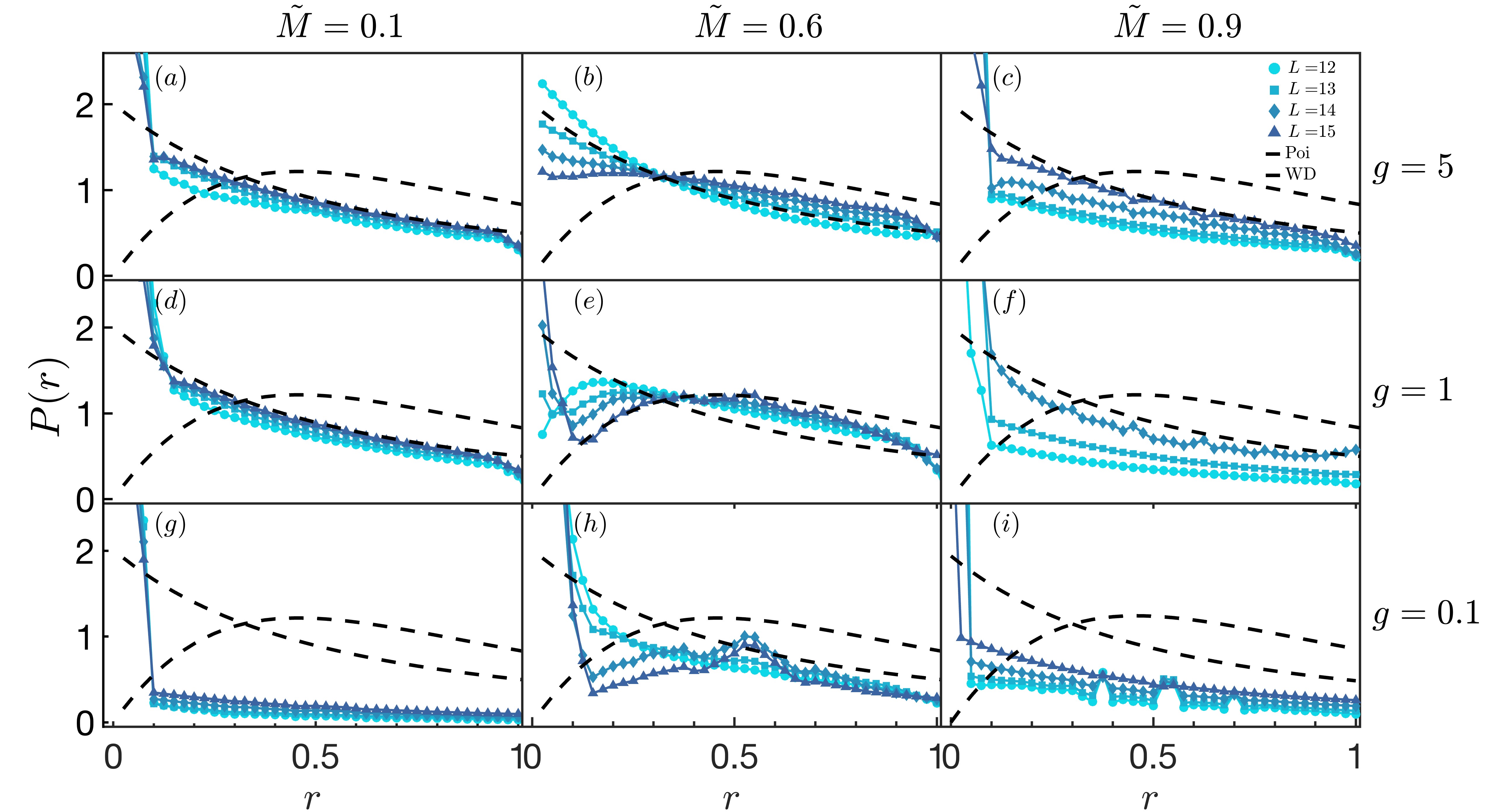
Figure 11: Level spacing ratio statistics for $g=0.1\,J,\,J,\,5\,J$, $\tilde{M}=0.1,\,0.6,\,0.9$ and $L=12,\,13,\,14,\,15$. The energy window $[0.3\,J,\,0.4\,J]$ was considered in the unfolded spectrum. Panels $(a)-(c)$: $g=5\,J$ displaying the perturbative breakdown of quantum chaos, remedied by the increasing system size. Restoration of quantum chaos happens slower for low and high $\tilde{M}$ in $(a)$ and $(c)$, respectively. Panels $(d)-(f)$: Similar behavior for $g=J$ with a faster restoration of quantum chaos for intermediate $\tilde{M}$. Panels $(g)-(i)$: $g=0.1\,J$ exhibiting similar features with an overall slower convergence towards the WD distribution.

Figure 12: Level velocity distributions for transverse field $g=0.25J,0.4J,0.6J$ with connectance $\tilde{M}=0.73,0.49,0.27$ in panels $(a)-(c)$ respectively. The system sizes ranging from small $L=11$ to large $L=15$ are considered here. The distributions depicted here do not exhibit unit variance because these plots serve to illustrate the shape of Gaussian curves, which become narrower as the system size increases.

Appendix D Spectral independence of local measures and slight deviations in the upper half of the spectrum

Figure 13: Level velocity distributions for $\tilde{M}=0.27,\,0.49$, $g=0.25\,J\,,0.4\,J\,,0.5\,J\,$ and $L=12,\,13,\,14,\,$ and $15$. The energy spectrum has been divided into $10$ energy windows. Panels $(a)-(c)$: $3^{\text{rd}},\,4^{\text{th}},\,8^{\text{th}},\,9^{\text{th}}$ energy windows. Panels $(d)-(f)$: windows $3^{\text{rd}},\,5^{\text{th}},\,7^{\text{th}},\,8^{\text{th}}$. Frustration in the upper half of the spectrum induces slight deviations ($4^{\text{th}},\,7^{\text{th}},\,8^{\text{th}}$ energy windows).

This appendix provides additional details about the spacing and velocity statistics, investigated separately in ten energy windows in the unfolded spectrum. As shown in Fig. 13 and Fig. 14, the upper half around the middle of the spectrum exhibits a slight deviation from the traditional spectral characteristics, whereas the lower half remains consistent with the local measures. As illustrated in Fig. 14, the level spacing distributions for $L=15$ show noticeable deviations compared to the lower half of the spectrum. In Fig. 14, spacing statistics in spectral regions $\tilde{E}\gtrsim J/2$ show additional peaks compared to the Poissonian and WD statistics, making it difficult to interpret the chaotic or integrable behavior of the spectrum. Moreover, the discrepancy from the chaotic behavior becomes more pronounced with increasing $L$ as shown in Fig. 13. The velocity statistics for $L=14,15$ deviate from the Gaussian distribution, whereas for $L=12,13$ it follows approximately a Gaussian shape throughout the spectrum. Nevertheless, the deviations that appear in the upper half in Fig. 13 are of different kinds compared to Fig. 4, Fig. 5, and Fig. 6. Here, the velocity distribution widens without any additional peaks, making it an efficient indicator of quantum chaos.

The observed deviations can be attributed to several factors. Frustrated loops can occur in connected graphs, leading to more degeneracies within the system. Additionally, certain graph configurations may involve nodes with even connectivity. Due to the uniform interaction strength, flipping these spins increases the number of degenerate excited states. These instances are more likely to occur around the middle of the spectrum at the highest density of states. The presence of degeneracies introduces a bias in the statistics, causing deviations from traditional spectral measures. In particular, the number of degenerate states is considerably lower for smaller $L$ compared to larger $L$.

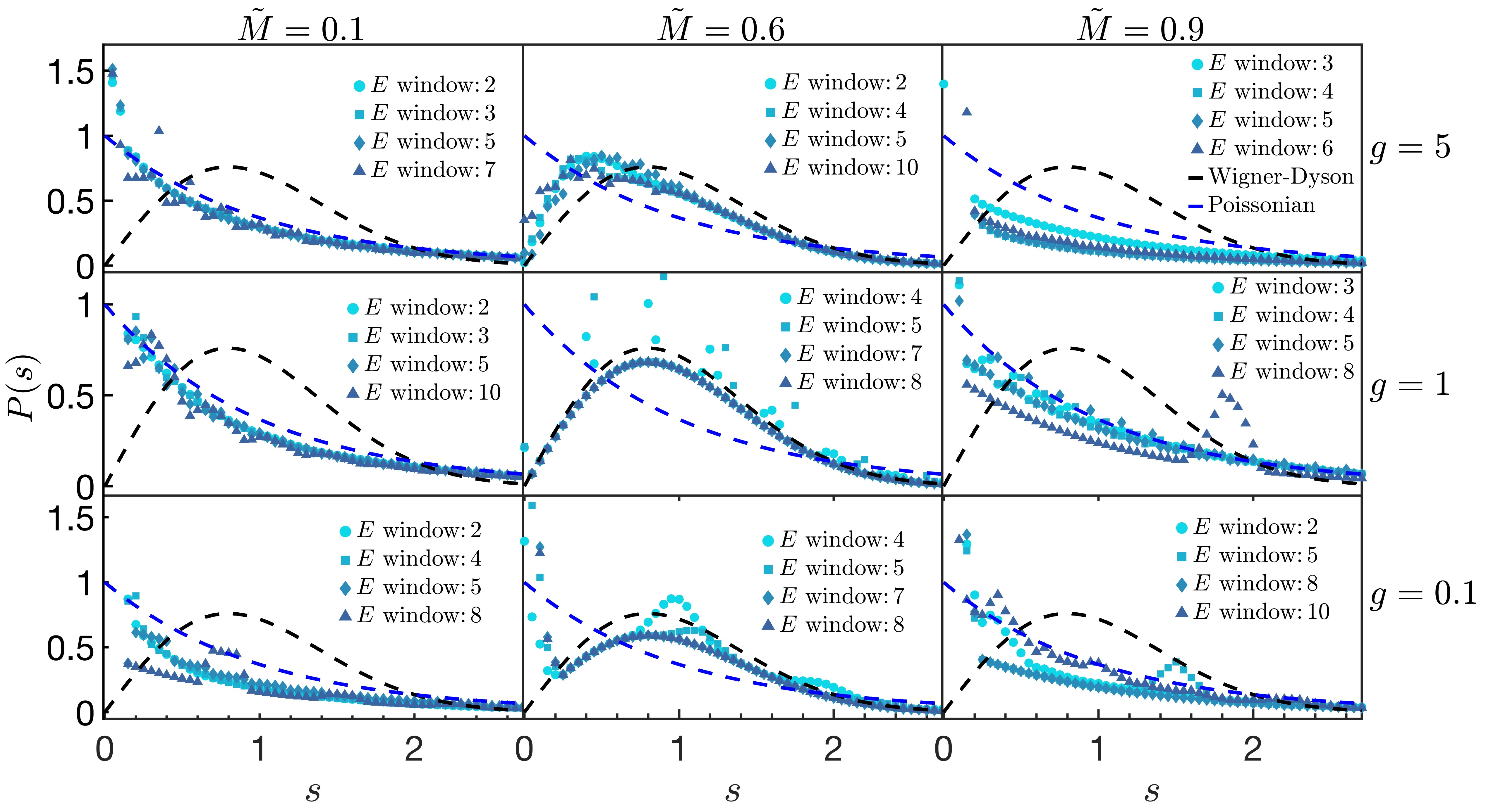
Figure 14: Level spacing statistics in different spectral windows with $\tilde{M}=0.1,\,0.6,\,0.9$, $g=0.1\,J,\,J,\,5\,J$ and $L=15$. Slight deviations are present in the upper half of the spectrum.

Appendix E Perturbative argument for the level velocity

The breakdown of the velocity statistics can be captured approximately using the first-order perturbation theory. Here, we limit our analysis to the non-degenerate cases as the degenerate spin configurations separated by one spin-flip emerge with a vanishingly small frequency of $1/\sqrt{L}$ in the thermodynamic limit, as discussed in Sec. B. For small $g$, $H_{x}$ acts as a perturbation to the unperturbed Hamiltonian $H_{P}$ in Eq. (1). Thus, the correction to the level velocity is given as,

$$v^{(1)}_{n}=\frac{1}{L}\bra{n}{H}_{x}\ket{\delta n}=\frac{gM}{L^{2}}\sum_{k\neq l}\frac{|\bra{l}{H}_{x}\ket{k}|^{2}}{\Delta E_{kl}},$$ (43)

where, $\ket{k}$ and $\ket{l}$ are energy eigenstates of ${H}_{P}$. Here, $\Delta E_{kl}/M=E_{k}-E_{l}$ as the energy spectrum is rescaled to $1/M$ with $E_{k}$ and $E_{l}$ denoting the eigenenergies. The average energy difference between two spin configurations separated by a unit Hamming distance scales approximately as $\Delta E_{kl}\sim S_{c}$. Here, $c=M/L$ is the average connectivity of a single node scaling as $\sim{L}$ in the connected limit. However, $S_{c}$ is the total spin of those connected nodes, falling within the range $[-L/2,+L/2]$. The most probable spin configurations in this interval scale as $\sim\sqrt{L}$. This is in agreement with Eq. (37), where both the average and fluctuation vary as $\sqrt{L}$. Moreover, for each spin configuration $\ket{k}$, there exist $L$ possible spin-flip configurations $\ket{l}$, where the matrix element $\bra{l}{H}_{x}\ket{k}$ is nonzero. Hence, Eq. (43) becomes,

$$v^{(1)}_{n}=\frac{gM}{L^{2}}\sum_{k\neq l}\frac{|\bra{l}{H}_{x}\ket{k}|^{2}}{\Delta E_{kl}}\sim\frac{gM}{L^{2}}\sum_{k=1}^{L}\pm\frac{1}{\sqrt{L}}\sim\frac{gM}{L^{2}}\frac{\sqrt{L}}{\sqrt{L}}.$$ (44)

The minus sign in the summation comes from the fact that the fluctuations dominate over the average. Due to the fluctuating sign but with the same order of magnitudes, the sum extends as $\sqrt{L}$. Using $\tilde{M}\sim M/L^{2}$ in the thermodynamic limit, Eq. (44) becomes,

$$v\sim g\sqrt{\tilde{M}}.$$ (45)

Now, let us investigate the opposite extreme, the fully polarized state. In this regime, the level velocity in Eq. (18) can be written as

$$v=\frac{1}{L}\bra{{n_{x}}}{H}_{x}\ket{{n_{x}}}=\frac{E_{n_{x}}}{L},$$ (46)

where, $\ket{n_{x}}$ is an $X$ polarized eigenstate of ${H}_{x}$ with eigenenergy $E_{nx}$. The spins in the paramagnetic phase can orient in $\pm X$ directions with $E_{nx}\in[-L/2,+L/2]$. The degree of degeneracy is given by binomial coefficients peaking at $E_{nx}=0$. This implies $E_{nx}\sim\sqrt{L}$ in the middle of the spectrum for large $g$. Thus, Eq. (46) becomes,

$$v\sim\frac{\sqrt{L}}{L}=\frac{1}{\sqrt{L}}.$$ (47)

References

- Lucas [2014] A. Lucas, Ising formulations of many np problems, Frontiers in Physics 2 (2014).
- Albash and Lidar [2018] T. Albash and D. A. Lidar, Adiabatic quantum computation, Rev. Mod. Phys. 90, 015002 (2018).
- Mézard et al. [1987] M. Mézard, G. Parisi, M. A. Virasoro, and D. J. Thouless, Spin glass theory and beyond (1987).
- Har [2005] Optimization problems in physics, in Phase Transitions in Combinatorial Optimization Problems (John Wiley and Sons, Ltd, 2005).
- Barahona [1982] F. Barahona, On the computational complexity of ising spin glass models, Journal of Physics A: Mathematical and General 15, 3241 (1982).
- Garey and Johnson [1979] M. Garey and D. Johnson, Computers and Intractability: A Guide to the Theory of NP-completeness, Mathematical Sciences Series (Freeman, 1979).
- Grimsley et al. [2019] H. R. Grimsley, S. E. Economou, E. Barnes, and N. J. Mayhall, An adaptive variational algorithm for exact molecular simulations on a quantum computer, Nature Communications 10, 3007 (2019).
- Bravo-Prieto et al. [2020] C. Bravo-Prieto, J. Lumbreras-Zarapico, L. Tagliacozzo, and J. I. Latorre, Scaling of variational quantum circuit depth for condensed matter systems, Quantum 4, 272 (2020).
- Di Meglio et al. [2023] A. Di Meglio, K. Jansen, I. Tavernelli, C. Alexandrou, S. Arunachalam, C. W. Bauer, K. Borras, S. Carrazza, A. Crippa, V. Croft, et al., Quantum computing for high-energy physics: State of the art and challenges. summary of the qc4hep working group, arXiv preprint arXiv:2307.03236 (2023).
- Barrat et al. [2008] A. Barrat, M. Barthélemy, and A. Vespignani, Contents, in Dynamical Processes on Complex Networks (Cambridge University Press, 2008).
- Watts and Strogatz [1998] D. J. Watts and S. H. Strogatz, Collective dynamics of ‘small-world’ networks, Nature 393, 440 (1998).
- Newman [2010] M. Newman, Networks: An Introduction (Oxford University Press, 2010).
- Dorogovtsev et al. [2002] S. N. Dorogovtsev, A. V. Goltsev, and J. F. F. Mendes, Ising model on networks with an arbitrary distribution of connections, Phys. Rev. E 66, 016104 (2002).
- Jeong et al. [2000] H. Jeong, B. Tombor, R. Albert, Z. N. Oltvai, and A.-L. Barabási, The large-scale organization of metabolic networks, Nature 407, 651–654 (2000).
- Montoya [2000] R. V. S. J. M. Montoya, Complexity and fragility in ecological networks (2000), arXiv:cond-mat/0011196 [cond-mat.dis-nn] .
- Garlaschelli et al. [2003] D. Garlaschelli, G. Caldarelli, and L. Pietronero, Universal scaling relations in food webs, Nature 423, 165 (2003).
- Bassett and Bullmore [2007] D. Bassett and E. Bullmore, Small-world brain networks, The Neuroscientist : a review journal bringing neurobiology, neurology and psychiatry 12, 512 (2007).
- Albert et al. [1999] R. Albert, H. Jeong, and A.-L. Barabási, Diameter of the world-wide web, Nature 401, 130 (1999).
- Erdos and Rényi [2022] P. L. Erdos and A. Rényi, On random graphs. i., Publicationes Mathematicae Debrecen (2022).
- Erdos and Rényi [1960] P. L. Erdos and A. Rényi, On the evolution of random graphs, Publications of the Mathematical Institute of the Hungarian Academy of Sciences (1960).
- Newman et al. [2001] M. E. J. Newman, S. H. Strogatz, and D. J. Watts, Random graphs with arbitrary degree distributions and their applications, Phys. Rev. E 64, 026118 (2001).
- Barabási and Albert [1999] A.-L. Barabási and R. Albert, Emergence of scaling in random networks, Science 286, 509 (1999).
- Bollobás [1985] B. Bollobás, Random Graphs, Cambridge studies in advanced mathematics (Academic Press, 1985).
- Farhi et al. [2001] E. Farhi, J. Goldstone, S. Gutmann, J. Lapan, A. Lundgren, and D. Preda, A quantum adiabatic evolution algorithm applied to random instances of an np-complete problem, Science 292, 472 (2001).
- Santoro et al. [2002] G. E. Santoro, R. Martoňák, E. Tosatti, and R. Car, Theory of quantum annealing of an ising spin glass, Science 295, 2427 (2002).
- Young et al. [2010] A. P. Young, S. Knysh, and V. N. Smelyanskiy, First-order phase transition in the quantum adiabatic algorithm, Phys. Rev. Lett. 104, 020502 (2010).
- Bapst et al. [2013] V. Bapst, L. Foini, F. Krzakala, G. Semerjian, and F. Zamponi, The quantum adiabatic algorithm applied to random optimization problems: The quantum spin glass perspective, Physics Reports 523, 127 (2013).
- Boixo et al. [2014] S. Boixo, T. F. Ronnow, S. V. Isakov, Z. Wang, D. Wecker, D. A. Lidar, J. M. Martinis, and M. Troyer, Evidence for quantum annealing with more than one hundred qubits, Nature Physics 10, 218 (2014).
- Kirkpatrick et al. [1983] S. Kirkpatrick, C. D. Gelatt, and M. P. Vecchi, Optimization by simulated annealing, Science 220, 671 (1983).
- Das et al. [2024] A. K. Das, P. Pinney, D. A. Zarate-Herrada, S. Pilatowsky-Cameo, A. S. Matsoukas-Roubeas, D. G. A. Cabral, C. Cianci, V. S. Batista, A. del Campo, E. J. Torres-Herrera, and L. F. Santos, Proposal for many-body quantum chaos detection (2024), arXiv:2401.01401 [cond-mat.stat-mech] .
- Šuntajs et al. [2020a] J. Šuntajs, J. Bonča, T. c. v. Prosen, and L. Vidmar, Ergodicity breaking transition in finite disordered spin chains, Phys. Rev. B 102, 064207 (2020a).
- Bulchandani et al. [2022] V. B. Bulchandani, D. A. Huse, and S. Gopalakrishnan, Onset of many-body quantum chaos due to breaking integrability, Phys. Rev. B 105, 214308 (2022).
- LeBlond et al. [2021] T. LeBlond, D. Sels, A. Polkovnikov, and M. Rigol, Universality in the onset of quantum chaos in many-body systems, Phys. Rev. B 104, L201117 (2021).
- Brown et al. [2008] W. G. Brown, L. F. Santos, D. J. Starling, and L. Viola, Quantum chaos, delocalization, and entanglement in disordered heisenberg models, Phys. Rev. E 77, 021106 (2008).
- Haake [2001] F. Haake, Quantum Signatures of Chaos, Vol. 54 (2001).
- Kos et al. [2018] P. Kos, M. Ljubotina, and T. c. v. Prosen, Many-body quantum chaos: Analytic connection to random matrix theory, Phys. Rev. X 8, 021062 (2018).
- Dubertrand and Müller [2016] R. Dubertrand and S. Müller, Spectral statistics of chaotic many-body systems, New Journal of Physics 18, 033009 (2016).
- Mehta [1991] M. Mehta, Random Matrices (Academic Press, 1991).
- Guhr et al. [1998] T. Guhr, A. Müller–Groeling, and H. A. Weidenmüller, Random-matrix theories in quantum physics: common concepts, Physics Reports 299, 189 (1998).
- Deutsch [1991] J. M. Deutsch, Quantum statistical mechanics in a closed system, Phys. Rev. A 43, 2046 (1991).
- Rigol et al. [2008] M. Rigol, V. Dunjko, and M. Olshanii, Thermalization and its mechanism for generic isolated quantum systems, Nature 452, 854 (2008).
- Deutsch [2018] J. M. Deutsch, Eigenstate thermalization hypothesis, Reports on Progress in Physics 81, 082001 (2018).
- Luca D’Alessio and Rigol [2016] A. P. Luca D’Alessio, Yariv Kafri and M. Rigol, From quantum chaos and eigenstate thermalization to statistical mechanics and thermodynamics, Advances in Physics 65, 239 (2016).
- Oganesyan and Huse [2007] V. Oganesyan and D. A. Huse, Localization of interacting fermions at high temperature, Phys. Rev. B 75, 155111 (2007).
- Abanin et al. [2019] D. A. Abanin, E. Altman, I. Bloch, and M. Serbyn, Colloquium: Many-body localization, thermalization, and entanglement, Rev. Mod. Phys. 91, 021001 (2019).
- Basko et al. [2006] D. Basko, I. Aleiner, and B. Altshuler, Metal–insulator transition in a weakly interacting many-electron system with localized single-particle states, Annals of Physics 321, 1126 (2006).
- Smith et al. [2016] J. Smith, A. Lee, P. Richerme, B. Neyenhuis, P. W. Hess, P. Hauke, M. Heyl, D. A. Huse, and C. Monroe, Many-body localization in a quantum simulator with programmable random disorder, Nature Physics 12, 907 (2016).
- Chaudhury et al. [2009] S. Chaudhury, A. Smith, B. E. Anderson, S. Ghose, and P. S. Jessen, Quantum signatures of chaos in a kicked top, Nature 461, 768 (2009).
- Panda et al. [2020] R. K. Panda, A. Scardicchio, M. Schulz, S. R. Taylor, and M. Žnidarič, Can we study the many-body localisation transition?, Europhysics Letters 128, 67003 (2020).
- Abanin et al. [2021] D. Abanin, J. Bardarson, G. De Tomasi, S. Gopalakrishnan, V. Khemani, S. Parameswaran, F. Pollmann, A. Potter, M. Serbyn, and R. Vasseur, Distinguishing localization from chaos: Challenges in finite-size systems, Annals of Physics 427, 168415 (2021).
- Kjäll et al. [2014] J. A. Kjäll, J. H. Bardarson, and F. Pollmann, Many-body localization in a disordered quantum ising chain, Phys. Rev. Lett. 113, 107204 (2014).
- Laumann et al. [2014] C. R. Laumann, A. Pal, and A. Scardicchio, Many-body mobility edge in a mean-field quantum spin glass, Phys. Rev. Lett. 113, 200405 (2014).
- G. and A. [2017] M. G. and S. A., Ergodic and localized regions in quantum spin glasses on the bethe lattice, Philosophical Transactions of the Royal Society A: Mathematical, Physical and Engineering Sciences 375, 160424201604 (2017).
- Mukherjee et al. [2018] S. Mukherjee, S. Nag, and A. Garg, Many-body localization-delocalization transition in the quantum sherrington-kirkpatrick model, Physical Review B 97, 10.1103/physrevb.97.144202 (2018).
- Mossi et al. [2017] G. Mossi, T. Parolini, S. Pilati, and A. Scardicchio, On the quantum spin glass transition on the bethe lattice, Journal of Statistical Mechanics: Theory and Experiment 2017, 013102 (2017).
- Kim et al. [2005] D.-H. Kim, G. J. Rodgers, B. Kahng, and D. Kim, Spin-glass phase transition on scale-free networks, Phys. Rev. E 71, 056115 (2005).
- Herrero [2009] C. P. Herrero, Antiferromagnetic ising model in scale-free networks, The European Physical Journal B 70, 435 (2009).
- Preethi and Dutta [2024] G. Preethi and S. Dutta, Frustrated quantum magnetism on complex networks: What sets the total spin (2024), arXiv:2403.09116 [cond-mat.dis-nn] .
- Viana Lopes et al. [2004] J. Viana Lopes, Y. G. Pogorelov, J. M. B. Lopes dos Santos, and R. Toral, Exact solution of ising model on a small-world network, Phys. Rev. E 70, 026112 (2004).
- Chatterjee and Sen [2006] A. Chatterjee and P. Sen, Phase transitions in an ising model on a euclidean network, Phys. Rev. E 74, 036109 (2006).
- Dorogovtsev et al. [2008] S. N. Dorogovtsev, A. V. Goltsev, and J. F. F. Mendes, Critical phenomena in complex networks, Rev. Mod. Phys. 80, 1275 (2008).
- Alt et al. [2021] J. Alt, R. Ducatez, and A. Knowles, Delocalization transition for critical erdős–rényi graphs, Communications in Mathematical Physics 388, 507 (2021).
- Sade et al. [2005] M. Sade, T. Kalisky, S. Havlin, and R. Berkovits, Localization transition on complex networks via spectral statistics, Phys. Rev. E 72, 066123 (2005).
- Benaych-Georges et al. [2017] F. Benaych-Georges, C. Bordenave, and A. Knowles, Largest eigenvalues of sparse inhomogeneous erdős-rényi graphs, The Annals of Probability 47 (2017).
- Cugliandolo et al. [2024] L. F. Cugliandolo, G. Schehr, M. Tarzia, and D. Venturelli, Multifractal phase in the weighted adjacency matrices of random erdös-rényi graphs (2024), arXiv:2404.06931 [cond-mat.dis-nn] .
- Smith et al. [2017] A. Smith, J. Knolle, R. Moessner, and D. L. Kovrizhin, Absence of ergodicity without quenched disorder: From quantum disentangled liquids to many-body localization, Phys. Rev. Lett. 119, 176601 (2017).
- Janarek et al. [2018] J. Janarek, D. Delande, and J. Zakrzewski, Discrete disorder models for many-body localization, Phys. Rev. B 97, 155133 (2018).
- Enss et al. [2017] T. Enss, F. Andraschko, and J. Sirker, Many-body localization in infinite chains, Phys. Rev. B 95, 045121 (2017).
- Periwal et al. [2021] A. Periwal, E. S. Cooper, P. Kunkel, J. F. Wienand, E. J. Davis, and M. Schleier-Smith, Programmable interactions and emergent geometry in an array of atom clouds, Nature 600, 630 (2021).
- King et al. [2023] A. D. King, J. Raymond, T. Lanting, R. Harris, A. Zucca, F. Altomare, A. J. Berkley, K. Boothby, S. Ejtemaee, C. Enderud, E. Hoskinson, S. Huang, E. Ladizinsky, A. J. R. MacDonald, G. Marsden, R. Molavi, T. Oh, G. Poulin-Lamarre, M. Reis, C. Rich, Y. Sato, N. Tsai, M. Volkmann, J. D. Whittaker, J. Yao, A. W. Sandvik, and M. H. Amin, Quantum critical dynamics in a 5,000-qubit programmable spin glass, Nature 617, 61 (2023).
- King et al. [2024] A. D. King, A. Nocera, M. M. Rams, J. Dziarmaga, R. Wiersema, W. Bernoudy, J. Raymond, N. Kaushal, N. Heinsdorf, R. Harris, K. Boothby, F. Altomare, A. J. Berkley, M. Boschnak, K. Chern, H. Christiani, S. Cibere, J. Connor, M. H. Dehn, R. Deshpande, S. Ejtemaee, P. Farré, K. Hamer, E. Hoskinson, S. Huang, M. W. Johnson, S. Kortas, E. Ladizinsky, T. Lai, T. Lanting, R. Li, A. J. R. MacDonald, G. Marsden, C. C. McGeoch, R. Molavi, R. Neufeld, M. Norouzpour, T. Oh, J. Pasvolsky, P. Poitras, G. Poulin-Lamarre, T. Prescott, M. Reis, C. Rich, M. Samani, B. Sheldan, A. Smirnov, E. Sterpka, B. T. Clavera, N. Tsai, M. Volkmann, A. Whiticar, J. D. Whittaker, W. Wilkinson, J. Yao, T. J. Yi, A. W. Sandvik, G. Alvarez, R. G. Melko, J. Carrasquilla, M. Franz, and M. H. Amin, Computational supremacy in quantum simulation (2024), arXiv:2403.00910 [quant-ph] .
- Lipkin et al. [1965] H. Lipkin, N. Meshkov, and A. Glick, Validity of many-body approximation methods for a solvable model: (i). exact solutions and perturbation theory, Nuclear Physics 62, 188 (1965).
- Altshuler et al. [2010] B. Altshuler, H. Krovi, and J. Roland, Anderson localization makes adiabatic quantum optimization fail, Proceedings of the National Academy of Sciences 107, 12446 (2010).
- Pal and Huse [2010] A. Pal and D. A. Huse, Many-body localization phase transition, Phys. Rev. B 82, 174411 (2010).
- Šuntajs et al. [2020b] J. Šuntajs, J. Bonča, T. c. v. Prosen, and L. Vidmar, Quantum chaos challenges many-body localization, Phys. Rev. E 102, 062144 (2020b).
- Bertrand and García-García [2016] C. L. Bertrand and A. M. García-García, Anomalous thouless energy and critical statistics on the metallic side of the many-body localization transition, Phys. Rev. B 94, 144201 (2016).
- Chirikov and Shepelyansky [1995] B. V. Chirikov and D. L. Shepelyansky, Shnirelman peak in level spacing statistics, Phys. Rev. Lett. 74, 518 (1995).
- Frahm and Shepelyansky [1997] K. M. Frahm and D. L. Shepelyansky, Quantum localization in rough billiards, Phys. Rev. Lett. 78, 1440 (1997).
- Zangara et al. [2013] P. R. Zangara, A. D. Dente, E. J. Torres-Herrera, H. M. Pastawski, A. Iucci, and L. F. Santos, Time fluctuations in isolated quantum systems of interacting particles, Phys. Rev. E 88, 032913 (2013).
- Vallejo-Fabila and Torres-Herrera [2022a] I. Vallejo-Fabila and E. J. Torres-Herrera, Effects of autocorrelated disorder on the dynamics in the vicinity of the many-body localization transition, Phys. Rev. B 106, L220201 (2022a).
- Pietracaprina et al. [2016] F. Pietracaprina, V. Ros, and A. Scardicchio, Forward approximation as a mean-field approximation for the anderson and many-body localization transitions, Phys. Rev. B 93, 054201 (2016).
- Anderson [1958] P. W. Anderson, Absence of diffusion in certain random lattices, Phys. Rev. 109, 1492 (1958).
- Abrahams et al. [1979] E. Abrahams, P. W. Anderson, D. C. Licciardello, and T. V. Ramakrishnan, Scaling theory of localization: Absence of quantum diffusion in two dimensions, Phys. Rev. Lett. 42, 673 (1979).
- Lee and Ramakrishnan [1985] P. A. Lee and T. V. Ramakrishnan, Disordered electronic systems, Rev. Mod. Phys. 57, 287 (1985).
- Altshuler et al. [1997] B. L. Altshuler, Y. Gefen, A. Kamenev, and L. S. Levitov, Quasiparticle lifetime in a finite system: A nonperturbative approach, Phys. Rev. Lett. 78, 2803 (1997).
- Sehrawat et al. [2021] A. Sehrawat, C. Srivastava, and U. Sen, Dynamical phase transitions in the fully connected quantum ising model: Time period and critical time, Phys. Rev. B 104, 085105 (2021).
- Yukawa [1985] T. Yukawa, New approach to the statistical properties of energy levels, Phys. Rev. Lett. 54, 1883 (1985).
- Pechukas [1983] P. Pechukas, Distribution of energy eigenvalues in the irregular spectrum, Phys. Rev. Lett. 51, 943 (1983).
- Braun and Montambaux [1994] D. Braun and G. Montambaux, Universal spectral correlations in diffusive quantum systems, Phys. Rev. B 50, 7776 (1994).
- Braun et al. [1997] D. Braun, E. Hofstetter, A. MacKinnon, and G. Montambaux, Level curvatures and conductances: A numerical study of the thouless relation, Phys. Rev. B 55, 7557 (1997).
- Thouless [1980] D. Thouless, Resistance and localization in thin films and wires, Journal of Non-Crystalline Solids 35-36, 3 (1980).
- Edwards and Thouless [1972] J. T. Edwards and D. J. Thouless, Numerical studies of localization in disordered systems, Journal of Physics C: Solid State Physics 5, 807 (1972).
- Akkermans and Montambaux [1992] E. Akkermans and G. Montambaux, Conductance and statistical properties of metallic spectra, Phys. Rev. Lett. 68, 642 (1992).
- Fyodorov and Mirlin [1995] Y. V. Fyodorov and A. D. Mirlin, Mesoscopic fluctuations of eigenfunctions and level-velocity distribution in disordered metals, Phys. Rev. B 51, 13403 (1995).
- Fyodorov [1994] Y. V. Fyodorov, Distribution of “level velocities” in quasi-1d disordered or chaotic systems with localization, Phys. Rev. Lett. 73, 2688 (1994).
- Simons and Altshuler [1993] B. D. Simons and B. L. Altshuler, Universalities in the spectra of disordered and chaotic systems, Phys. Rev. B 48, 5422 (1993).
- Simons et al. [1993] B. D. Simons, A. Szafer, and B. L. Altshuler, Universality in quantum chaotic spectra, Pis’ma v Zhurnal Ehksperimental’noj i Teoreticheskoj Fiziki 57, 268 (Mar 1993).
- Maksymov et al. [2019] A. Maksymov, P. Sierant, and J. Zakrzewski, Energy level dynamics across the many-body localization transition, Phys. Rev. B 99, 224202 (2019).
- Grabarits [2023] A. Grabarits, Level dynamics and avoided level crossings in driven disordered quantum dots, Phys. Rev. B 107, 014206 (2023).
- Wilkie and Brumer [1991] J. Wilkie and P. Brumer, Time-dependent manifestations of quantum chaos, Phys. Rev. Lett. 67, 1185 (1991).
- Leviandier et al. [1986] L. Leviandier, M. Lombardi, R. Jost, and J. P. Pique, Fourier transform: A tool to measure statistical level properties in very complex spectra, Phys. Rev. Lett. 56, 2449 (1986).
- Alhassid and Whelan [1993] Y. Alhassid and N. Whelan, Onset of chaos and its signature in the spectral autocorrelation function, Phys. Rev. Lett. 70, 572 (1993).
- Sierant and Zakrzewski [2020] P. Sierant and J. Zakrzewski, Model of level statistics for disordered interacting quantum many-body systems, Phys. Rev. B 101, 104201 (2020).
- Gharibyan et al. [2018] H. Gharibyan, M. Hanada, S. H. Shenker, and M. Tezuka, Onset of random matrix behavior in scrambling systems, Journal of High Energy Physics 2018, 124 (2018).
- Prakash et al. [2021] A. Prakash, J. H. Pixley, and M. Kulkarni, Universal spectral form factor for many-body localization, Phys. Rev. Res. 3, L012019 (2021).
- Cao et al. [2022] Z. Cao, Z. Xu, and A. del Campo, Probing quantum chaos in multipartite systems, Phys. Rev. Res. 4, 033093 (2022).
- Joshi et al. [2022] L. K. Joshi, A. Elben, A. Vikram, B. Vermersch, V. Galitski, and P. Zoller, Probing many-body quantum chaos with quantum simulators, Phys. Rev. X 12, 011018 (2022).
- Roy et al. [2022] D. Roy, D. Mishra, and T. c. v. Prosen, Spectral form factor in a minimal bosonic model of many-body quantum chaos, Phys. Rev. E 106, 024208 (2022).
- del Campo et al. [2017] A. del Campo, J. Molina-Vilaplana, and J. Sonner, Scrambling the spectral form factor: Unitarity constraints and exact results, Phys. Rev. D 95, 126008 (2017).
- Távora et al. [2017] M. Távora, E. J. Torres-Herrera, and L. F. Santos, Power-law decay exponents: A dynamical criterion for predicting thermalization, Phys. Rev. A 95, 013604 (2017).
- del Campo et al. [2018] A. del Campo, J. Molina-Vilaplana, L. F. Santos, and J. Sonner, Decay of a thermofield-double state in chaotic quantum systems, The European Physical Journal Special Topics 227, 247 (2018).
- Schiulaz et al. [2019] M. Schiulaz, E. J. Torres-Herrera, and L. F. Santos, Thouless and relaxation time scales in many-body quantum systems, Phys. Rev. B 99, 174313 (2019).
- Vallejo-Fabila and Torres-Herrera [2022b] I. Vallejo-Fabila and E. J. Torres-Herrera, Effects of autocorrelated disorder on the dynamics in the vicinity of the many-body localization transition, Phys. Rev. B 106, L220201 (2022b).
- Cotler et al. [2017] J. S. Cotler, G. Gur-Ari, M. Hanada, J. Polchinski, P. Saad, S. H. Shenker, D. Stanford, A. Streicher, and M. Tezuka, Black holes and random matrices, Journal of High Energy Physics 2017, 118 (2017).