State-Constrained Offline Reinforcement Learning

Abstract

Traditional offline reinforcement learning methods predominantly operate in a batch-constrained setting. This confines the algorithms to a specific state-action distribution present in the dataset, reducing the effects of distributional shift but restricting the algorithm greatly. In this paper, we alleviate this limitation by introducing a novel framework named state-constrained offline reinforcement learning. By exclusively focusing on the dataset’s state distribution, our framework significantly enhances learning potential and reduces previous limitations. The proposed setting not only broadens the learning horizon but also improves the ability to combine different trajectories from the dataset effectively, a desirable property inherent in offline reinforcement learning. Our research is underpinned by solid theoretical findings that pave the way for subsequent advancements in this domain. Additionally, we introduce StaCQ, a deep learning algorithm that is both performance-driven on the D4RL benchmark datasets and closely aligned with our theoretical propositions. StaCQ establishes a strong baseline for forthcoming explorations in state-constrained offline reinforcement learning.

1 Introduction

Offline reinforcement learning (RL) focuses on deriving an optimal decision-making policy from a fixed dataset of previously collected experiences [36, 38]. It prohibits online exploration, meaning that effective policies must be constructed solely from the evidence provided by an unknown, potentially sub-optimal behaviour policy active in the environment. This approach is especially suited for real-world scenarios where executing sub-optimal actions can be dangerous, time-consuming, or costly, yet there is an abundance of prior data. Relevant applications include robotics [46, 34, 47], long-term healthcare treatment plans [51, 50, 44], and autonomous driving [43, 18, 16]. Despite its practical appeal, offline RL faces a significant challenge called distributional shift [33]. This phenomenon arises when attempting to estimate the values of actions not present in the dataset, often manifesting as an overestimation. As a result, out-of-distribution (OOD) actions are perceived as more valuable than they truly are, causing the agent to select sub-optimal actions and leading to the accumulation of errors [22].

Currently available offline RL techniques mitigate the issue of distributional shift through two primary approaches. The first confines the policy to produce only actions likely to emerge from the dataset or its distribution [22, 33, 55, 45, 31, 63, 21]. The second approach revolves around conservatively estimating the value of OOD actions [35, 58, 3]. Both strategies aim to anchor the learning algorithm to the state-action pairs within the dataset, an approach termed batch-constrained [22]. By doing so, these methods seek to minimise the impact of distributional shift. However, adhering strictly to the state-action distribution can be restrictive. Thus, recent techniques seek a balance between exploiting potentially valuable OOD actions and minimising distributional shift repercussions.

Given the constraints of the state-action distribution, a pivotal question arises: can we confine our methods to the state distribution alone and still counteract distributional shift?

Constraining exclusively to the dataset’s state distribution could significantly reduce the requisite dataset size. Instead of needing all state-action pairs, the focus shifts to states alone. This approach allows the agent to initiate out-of-distribution (OOD) actions, provided they lead to a known state. Such flexibility can enhance the capability of offline RL algorithms in trajectory stitching—combining sub-optimal experiences into improved trajectories. Rather than connecting based on actions from different trajectories, the state-constrained approach facilitates stitching by leveraging adjacent states. This method relies on understanding these proximate states, a concept we label as reachability. This concept refers to the ability to reach a particular state from another state within the dataset. In the state-constrained approach, understanding reachability is crucial for effectively stitching together sub-optimal trajectories and improving the overall policy. In some environments, reachability is easily delineated; for example, in grid-based environments like mazes, where the agent can move directly between adjacent cells. In other environments, reachability must be ascertained from the dataset, such as in complex robotic systems where state transitions depend on intricate dynamics.

Building upon the concept of reachability, in this paper, we develop a state-constrained offline RL approach and make several contributions to this new area. In the batch-constrained approach, the learning algorithm is anchored to the state-action pairs within the dataset. In contrast, the state-constrained approach focuses solely on the states, allowing for more flexibility in action selection while still mitigating distributional shift. We provide our state-constrained framework with theoretical guarantees, built on a few foundational assumptions. We demonstrate that the state-constrained framework will always construct a policy that produces higher or equal-value actions compared to the batch-constrained policy. Finally, we propose and empirically validate a novel deep state-constrained offline RL algorithm, called StaCQ. StaCQ learns a state-constrained Q-function and updates the policy to remain close to the highest quality reachable states within the dataset. Our experiments show that StaCQ demonstrates competitive performance, outperforming several state-of-the-art methods on the D4RL benchmarking dataset [20] in many tasks. StaCQ outperforms all model-free baselines in the locomotion tasks and shows strong performance in the Antmaze tasks. These results provide a strong basis for many future state-constrained algorithms to be built upon. We believe that this work will serve as a foundation for the development of future state-constrained algorithms, much like how BCQ [22] has done for batch-constrained techniques, and contribute to the advancement of offline RL.

2 Related work

Model-free offline RL.

BCQ [22] emerged as one of the pioneer offline deep RL methodologies. It posits that possessing all $(s,a)$-pairs in the MDP allows for constructing an optimal QA-value by narrowing the update solely to $(s,a)$-pairs present in the dataset. Consequently, BCQ restricts the policy to $(s,a)$-pairs in the dataset while allowing minimal perturbations to facilitate marginal benefits. Post-BCQ, numerous algorithms have been proposed to devise alternative means to limit the policy to $(s,a)$-pairs in the dataset, be it in the support of the $(s,a)$-distribution [33, 55, 45, 31, 63, 8] or directly to the $(s,a)$-pairs [21]. In a distinct vein, instead of policy constraints, certain methods have sought to circumvent distributional shifts by pessimistically evaluating the value function on out-of-distribution $(s,a)$-pairs [35, 58, 3]. A subset of offline RL methodologies both pessimistically evaluate the value function and constrain the policy [14, 7]. Both clusters of methods adopt the batch-constrained approach which prioritises $(s,a)$-pairs in the dataset over unobserved actions. Our state-constrained method eases the batch-constrained objective, necessitating constraint only to dataset states rather than $(s,a)$-pairs.

Model-based offline RL.

Model-based methods learn the dynamics of the environment to aid policy learning [48, 28]. There is usually two main approaches to model-based offline RL. The first approach learns a pessimistic model of the environment and performs rollouts using this augmented model, increasing the dataset size [59, 29, 42]. The other main approach aims to use the models to perform planning [4, 60, 27, 15]. This means that, during evaluation the models are used to look in the future to decide the optimal path for the agent. In contrast, StaCQ uses the models to implement our notion of state reachability. This means that the models are not used to imagine new states, and there is no planning involved at evaluation.

State reachability.

The state-constrained strategy heavily leans on state reachability. Earlier studies have explored state reachability [25, 26], with a Gaussian distribution determining the stitching feasibility of $s^{\prime}$ from $s$. Our approach, in contrast, deems a state as either reachable or not, steering clear of continuous probability distributions. The notion of state reachability aligns with state similarity, a subject of extensive study in literature [61, 1, 37]. One technique to gauge state similarity is through bisimulation metrics grounded in the environment’s dynamics [19]. Bisimulations usually mandate full state enumeration [11, 5, 6], prompting the introduction of a scalable pseudometric approach [10]. Integrating a pseudometric into our state reachability concept would be intriguing, but such exploration is deferred to future research. Our metric for state reachability is intuitively graspable and stems directly from the foundational definition.

Trajectory stitching.

Offline RL’s hallmark is its stitching capability [32]. This entails amalgamating previously observed trajectories to produce a novel trajectory that accomplishes the task. Imitation learning strategies, such as behavioural cloning (BC) [40, 41], are ineffective at stitching, given their inability to discern between optimal and sub-optimal states. Analogous to BC, the Decision transformer (DT)[12] converts the offline RL challenge into a supervised learning task by employing a goal-conditioned policy. Despite DT’s deficient stitching capabilities, efforts have been undertaken to rectify this by incorporating offline RL characteristics [57, 56]. Integrating DT with the policy extraction method of StaCQ may offer potential insights into enhancing stitching capabilities. However, our present study is squarely centred on a basic implementation of state-constrained offline RL.

3 Preliminaries

The RL framework involves an agent interacting with an environment, which is typically represented as a Markov Decision Process (MDP). Such an MDP is defined as $\mathcal{M}=(\mathcal{S},\mathcal{A},P,R,\gamma)$, where $\mathcal{S}$ and $\mathcal{A}$ denote the state and action spaces, respectively; $P=p(s^{\prime}|s,a)$ represents the environment transition dynamics; $R=r(s,a,s^{\prime})$ is the reward function for transitioning; and $0\leq\gamma<1$ is the discount factor [49]. We focus on the deterministic MDP, where $p(s^{\prime}|s,a)=\{0,1\}$ and $r(s,a,s^{\prime})=r(s,s^{\prime})$. In RL, the agent’s objective is to identify an optimal policy, $\pi(s)$, that maximises the future discounted sum of rewards $\sum_{i=t}\gamma^{i-t}r_{i}(s_{i},s^{\prime}_{i})$.

QA-values, $Q(s,a)=\mathbb{E}_{\pi}[\sum_{i=0}\gamma^{t}r_{t}(s_{t},a_{t})|s_{0}=s,a_{0}=a]$, are the expected future discounted rewards for executing action $a$ in state $s$ and there after following policy $\pi$. Q-learning [54], denoted as QA-learning in this paper, estimates the QA-values under the assumption that future actions are chosen optimally,

$$Q(s,a)\leftarrow(1-\alpha)Q(s,a)+\alpha\Bigl{[}r(s,a,s^{\prime})+\gamma\max_{a^{\prime}}Q(s^{\prime},a^{\prime})\Bigr{]}.$$ (1)

The optimal policy derived from QA-learning identifies the best action that maximises the QA-values, $\pi^{*}(s)=\text{arg}\max_{a}Q(s,a)$. In deterministic contexts, QA-learning parallels QS-learning [17], which estimates the expected rewards upon transitioning from state $s$ to $s^{\prime}$, followed by optimal decisions:

$$Q(s,s^{\prime})\leftarrow(1-\alpha)Q(s,s^{\prime})+\alpha\Bigl{[}r(s,s^{\prime})+\gamma\max_{s^{\prime\prime}}Q(s^{\prime},s^{\prime\prime})\Bigr{]}.$$ (2)

QS-learning enables QS-values to be learned for transitioning, without evaluating actions. The optimal policy via QS-learning discerns the most advantageous subsequent state to maximise QS-values, $\pi_{s}^{*}(s)=\text{arg}\max_{s^{\prime}}Q(s,s^{\prime})$. An action can then be retrieved from an inverse dynamics model as $a=I(s,\pi_{s}^{*}(s))$, a strategy designed to address QA-learning’s challenges in redundant action spaces. Redundant action spaces refer to situations where multiple actions lead to the same next state, making it challenging for QA-learning to distinguish between them.

In offline RL, the agent aims to discover an optimal policy; however, it must solely rely on a fixed dataset without further interactions with the environment [36, 38]. The dataset comprises trajectories made up of transitions consisting of the current state, action, next state, and the reward for transitioning, where actions are chosen based on an unknown behaviour policy, $\pi_{\beta}$. Batch-Constrained QA-learning (BCQL) [22] adapts QA-learning for the offline setting by restricting the optimisation to state-action pairs present in the dataset:

$$Q(s,a)\leftarrow(1-\alpha)Q(s,a)+\alpha\Bigl{[}r(s,a,s^{\prime})+\gamma\max_{a^{\prime}\text{s.t.}(s^{\prime},a^{\prime})\in\mathcal{D}}Q(s^{\prime},a^{\prime})\Bigr{]}.$$ (3)

This approach is restrictive since convergence to the optimal value function is only ensured if every conceivable $(s,a)$-pair from the MDP resides within the dataset. Such a limitation aims to sidestep extrapolation errors resulting from distributional shifts. Nonetheless, this framework places a significant constraint on any learning algorithm. Subsequent sections relax this constraint: instead of adhering strictly to state-action pairs (batch-constrained), the learning process is only bound by states (state-constrained). In the following section, we introduce the state-constrained framework and provide a new algorithm called state-constrained QS-learning (SCQL). We show that, under minor assumptions, SCQL converges to the optimal QS-value and produces a less-restrictive policy than BCQL.

4 State-constrained QS-learning

In this section, we provide a formal introduction to state-constrained QS-learning and establish its convergence to the optimal QS-value under a set of minimal assumptions. Within this framework, the learning updates are restricted exclusively to the states present in the dataset. A rigorous definition of state reachability is indispensable for this setting:

Definition 4.1.

(State reachability) In a deterministic MDP $\mathcal{M}$, a state $s^{\prime}$ is considered reachable from state $s$ if and only if there exists an action $a$ such that $p(s^{\prime}|s,a)=1$. We denote the set of states reachable from $s$ as $\mathcal{SR}_{\mathcal{M}}(s)$, where $s^{\prime}\in\mathcal{SR}_{\mathcal{M}}(s)$.

Definition 4.1 implies that a state is reachable if there exists an action that, when executed in the environment, leads to that state. This definition allows multiple reachable next states to be evaluated rather than a single state-action pair. By evaluating multiple reachable next states, state-constrained QS-learning allows for more flexibility in the learning updates compared to batch-constrained approaches, which are limited to evaluating only existing state-action pairs in the dataset.

4.1 Theory

In this section, we initially adapt the theorems presented in BCQL [22] to suit the state-constrained context (Theorems 4.4 - 4.6). All our subsequent theorems are based on QS-learning. However, it is important to note that these theorems still hold if QA-learning is used instead, with an inverse model defined to evaluate actions between states and reachable next states.

Our theory operates under the following assumptions: (A1) the environment is deterministic; (A2) the rewards are bounded such that $\forall(s,s^{\prime}),|r(s,s^{\prime})|\leq c$; (A3) the QS-values, $Q(s,s^{\prime})$, are initialised to finite values; and (A4) the discount factor is set such that $0\leq\gamma<1$.

First, we show that under these assumptions, QS-learning converges to the expert QS-value.

Theorem 4.2.

Under assumptions A1-4, and with the training rule given by

$$Q(s,s^{\prime})\leftarrow r(s,s^{\prime})+\gamma\max_{s^{\prime\prime}\text{ s.t. }s^{\prime\prime}\in\mathcal{SR}_{\mathcal{M}}(s^{\prime})}Q(s^{\prime},s^{\prime\prime}),$$ (4)

assuming each $(s,s^{\prime})$ pair is visited infinitely often, then as updates are performed, the agent’s hypothesis $Q_{n}(s,s^{\prime})$ after the $n$th update converges to the expert QS-value, $Q^{*}(s,s^{\prime})$, as $n\rightarrow\infty$ for all $s,s^{\prime}$.

Proof.

This follows from the convergence of QA-learning in a deterministic MDP [39]. For brevity and clarity, the full proof is shown in the Appendix. ∎

The convergence of QS-learning in a deterministic MDP, as shown in Theorem 4.2, is crucial for establishing the convergence of SCQL. Since SCQL is based on QS-learning and operates in a deterministic MDP, Theorem 4.2 provides the foundation for proving the convergence and optimality of SCQL under certain assumptions. We now demonstrate that learning the value function from the dataset $\mathcal{D}$ is equivalent to determining the value function of an associated MDP, denoted as $\mathcal{M}_{\mathcal{S}}$. Intuitively, $\mathcal{M}_{\mathcal{S}}$ is the MDP where all transitions are possible between reachable states found in $\mathcal{D}$.

Definition 4.3.

(State-constrained MDP) Let the state-constrained MDP $\mathcal{M}_{\mathcal{S}}=(\mathcal{S},\mathcal{A},\mathcal{P}_{\mathcal{S}},\mathcal{R},\gamma)$. Here, both $\mathcal{S}$ and $\mathcal{A}$ remain identical to those in the original MDP, $\mathcal{M}$. The transition probability is given by: $a=I(s,s^{\prime})\in\mathcal{A}$

$$p_{\mathcal{S}}(s^{\prime}|s,a)=\begin{cases}1&\text{if }(s,s^{\prime}\in\mathcal{D}\text{ and }s^{\prime}\in\mathcal{SR}_{\mathcal{M}}(s))\text{ or }(s\notin\mathcal{D}\text{ and }s^{\prime}=s_{\text{terminal}})\\ 0&\text{otherwise.}\end{cases}$$ (5)

The reward function and discount factor remain the same as the original MDP.

The transition probability $p_{\mathcal{S}}(s^{\prime}|s,a)$ in the state-constrained MDP is defined such that transitions are possible only between states that are reachable from each other according to the state reachability definition. This ensures that the state-constrained MDP captures the essential dynamics of the original MDP while focusing on the states present in the dataset. The reward $r(s,s^{\prime})$ is assigned as the original reward defined in $\mathcal{M}$. Note that such states $s$ and $s^{\prime}$ may not exist as a pair $(s,s^{\prime})$ in $\mathcal{D}$. For the case where $s$ is absent from the dataset, the rewards are set to the initialised values $Q(s,s^{\prime})$. Importantly, the $s$ and $s^{\prime}$ in Definition 4.3 both exist in the dataset but not as a pair; this means that more transitions exist under this definition than in the batch-constrained MDP defined in [22].

Theorem 4.4.

By sampling $s$ from the dataset $\mathcal{D}$, sampling $s^{\prime}$ from $\mathcal{SR}_{\mathcal{M}}(s)$ and performing QS-learning on all reachable state-next state pairs, QS-learning converges to the optimal value function of the state-constrained MDP $\mathcal{M}_{\mathcal{S}}$.

Proof.

Given in Appendix A. ∎

Theorem 4.4 establishes that performing QS-learning on all reachable state-next state pairs from the dataset converges to the optimal value function of the state-constrained MDP. This result is crucial for understanding the convergence and optimality properties of SCQL, as it shows that QS-learning effectively learns the optimal value function of the state-constrained MDP, which is closely related to the original MDP. We are now ready to define the state-constrained QS-learning (SCQL) update which is similar to the BCQL formulation except now the maximisation is constrained to the states rather than state-action pairs in the dataset. This formulation allows the maximisation to be taken over more values composing more accurate Q-values while still staying close to the dataset:

$$Q(s,s^{\prime})\leftarrow(1-\alpha)Q(s,s^{\prime})+\alpha\Bigl{[}r(s,s^{\prime})+\gamma\max_{\begin{subarray}{c}s^{\prime\prime}s.t.s^{\prime\prime}\in\mathcal{D}\\ s^{\prime\prime}\in\mathcal{SR}_{\mathcal{M}}(s^{\prime})\end{subarray}}Q(s^{\prime},s^{\prime\prime})\Bigr{]}.$$ (6)

SCQL, Eq. (6), converges under the identical conditions as traditional QS-learning, primarily because the state-constrained setting is non-limiting whenever every state in the MDP is observed.

Theorem 4.5.

Under assumptions A1-4 and assuming every state $s$ is encountered infinitely, SCQL converges to the optimal value function, denoted as $Q^{*}$.

Proof.

This follows from Theorem 4.2, noting the state-constraint is non-restrictive with a dataset which contains all possible states. ∎

Theorem 4.5 is a reduction in the restriction compared to BCQL as now we only require every state to be encountered infinitely rather than every $(s,a)$ -pair.

The optimal policy for our state-constrained approach can be formulated as:

$$\pi_{s}^{*}(s)=\mathop{\arg\max}\limits_{\begin{subarray}{c}s^{\prime}~{}\mathrm{s.t.}s^{\prime}\in\mathcal{D}\\ s^{\prime}\in\mathcal{SR}_{\mathcal{M}}(s)\end{subarray}}Q^{*}(s,s^{\prime}).$$ (7)

Here, the maximisation is taken over next states from the dataset and that are reachable from the current state. We now demonstrate that Eq. (7) represents the optimal state-constrained policy.

Theorem 4.6.

Under assumptions A1-4 and assuming every $s$ is visited infinitely, then SCQL converges to $Q^{\pi}_{\mathcal{S}}(s,s^{\prime})$, with the optimal state-constrained policy defined by Eq. (7) and $s^{\prime}\in\mathcal{SR}_{\mathcal{M}}(s)$.

Proof.

Given in Appendix A. ∎

Theorem 4.6 has important practical implications for the performance of SCQL in real-world scenarios with limited datasets. It suggests that SCQL can learn an optimal state-constrained policy even when the dataset does not contain all possible state-action pairs, as long as every state is visited infinitely often. The state-constrained approach greatly reduces the limitations placed on the learning algorithm compared to the batch-constrained method. In the batch-constrained approach, the necessity for every state-action pair to be present in the dataset demands a dataset of size at least $|\mathcal{S}|\times|\mathcal{A}|$. On the other hand, the state-constrained method only mandates that each state be visited, which minimally requires a dataset size of $|\mathcal{S}|$.

We will now show that BCQL is a special case of SCQL, and that policies produced by SCQL will never be worse than policies produced by BCQL.

Theorem 4.7.

In a deterministic MDP, SCQL will produce a policy that is never worse than the policy produced by BCQL.

Proof.

Given in Appendix A. ∎

From Theorems 4.6 and 4.7, the state-constrained approach poses fewer restrictions than the batch-constrained counterpart while also always producing a policy at least as good. SCQL can perform more Q-value updates and maximize over more states than BCQL because it considers all reachable state-next state pairs from the dataset, rather than being limited to the explicit state-action pairs present in the dataset. This allows SCQL to exploit the structure of the state-constrained MDP more effectively and learn a better policy, with less required data. In the next section, this improvement is elaborated through an illustrative example which shows SCQL excelling even with a limited dataset.

4.2 An illustrative example: maze navigation

To elucidate the advantages of SCQL in comparison to BCQL, we explore a simple maze environment backed by a dataset with few trajectories. The maze is visualised as a $10$ by $10$ grid. The available states are shown as white squares, while the red squares represent the maze walls. Each state in this environment is denoted by the $(x,y)$ coordinates within the maze, and the agent’s available actions comprise of simple movements: left, right, up, and down. With each movement, the agent incurs a reward penalty of a small negative value, but upon successfully navigating to the gold star, it is rewarded with a large positive value. Consequently, the agent’s primary objective becomes devising the most direct route to the star. In this deterministic environment, the outcomes of transitioning to a state and executing an action are congruent, meaning Eq. (1) and (2) mirror each other. This allows for a direct comparison between BCQL and SCQL in terms of their performance and ability to leverage limited datasets.

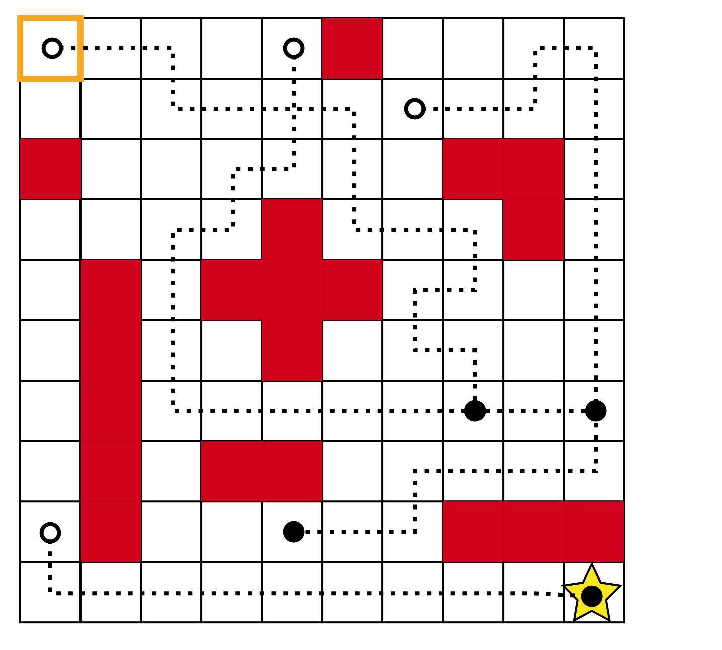
(a) Maze and Dataset

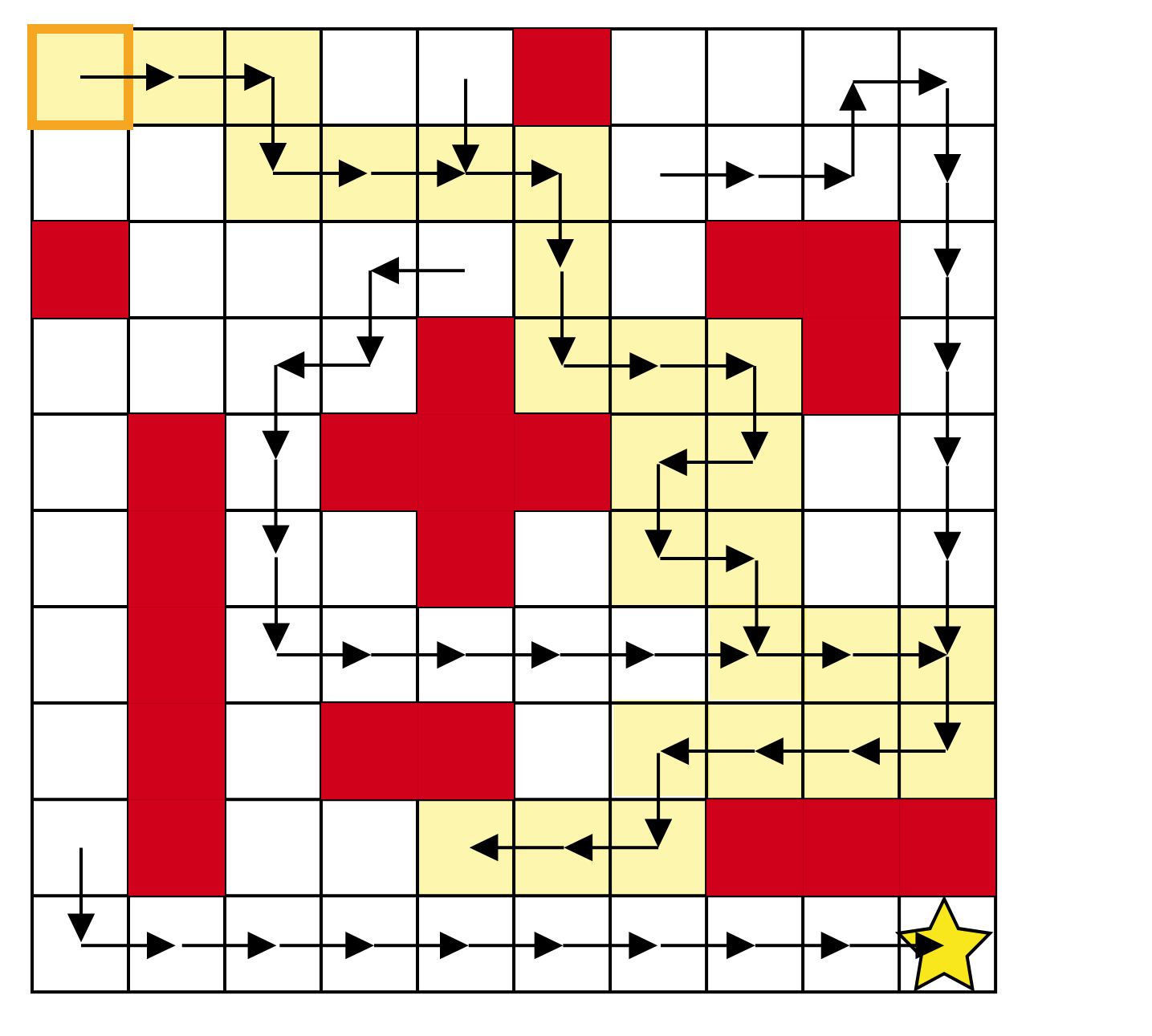
(b) BCQL Final Policy

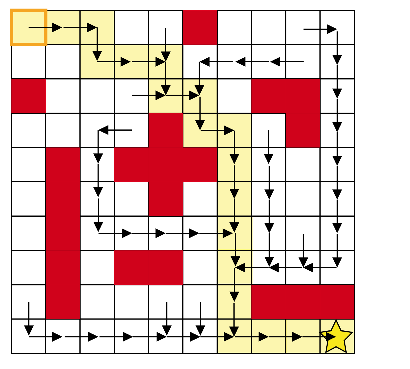
(c) SCQL Final Policy

Figure 1: Comparison of BCQL and SCQL methods on a simple maze environment. (a) The maze is a 10 by 10 grid where the co-ordinate values $(x,y)$ represent the state. The high reward region is represented by a star and maze walls are represented by red grid squares. The dataset is made of 4 trajectories represented by the dotted lines where the open circle is the starting state and the closed circle is the final state. (b) The final policy when applying BCQL to the dataset. (c) The final policy when applying SCQL to the dataset.

Figure 1a provides a visual representation of the maze and accompanying dataset. Here, trajectories start at the white circle and end at the black one. Despite its simplicity, the dataset contains a scant number of states wherein multiple actions have been taken. Within this specific framework, the notion of state reachability is straightforward: any state that is just one block away from the current state is considered reachable. Formally the state reachability is, $\mathcal{SR}_{\mathcal{M}}((x,y))=\{(x+1,y),(x-1,y),(x,y+1),(x,y-1)\}$. In other words, a state is considered reachable from the current state if it is one block away in any of the four cardinal directions (left, right, up, or down). This simple definition of state reachability is sufficient for demonstrating the advantages of SCQL in this illustrative example.

Applying BCQL with training as per Eq. (3) and policy extraction as per

$$\pi(s)=\max_{a\text{ s.t. }(s,a)\in\mathcal{D}}Q(s,a),$$

we obtain the policy depicted in Figure 1b, where arrows indicate policy direction. Conversely, for SCQL, training via Eq. (6) and policy training through Eq. (7) yields the policy in Figure 1c. For clarity, if no optimal movement can be found in the state, due to no information in the dataset, it is left blank. SCQL is able to leverage the sparse dataset more efficiently, enabling the agent to reach the gold star from any dataset state position. In contrast, BCQL succeeds in only 11 of the 57 unique dataset states, this is equivalent to behavioural cloning’s performance. SCQL’s advantage stems from its ability to leverage state adjacency information to stitch together optimal trajectories, whereas BCQL relies solely on previously observed state-action pairs, limiting its performance in datasets with a small number of trajectories.

5 Practical implementation: StaCQ

In this section, we introduce StaCQ (State-Constrained deep QS-learning), our particular deep learning implementation of SCQL. We present a policy constraint method that regularises the policy towards the best reachable next state in the dataset. Our specific implementation learns a QS-function that is aligned with the underlying theory. However, state-constrained methods could be adapted from the theory in many ways, analogous to many techniques that modify the batch-constraint for enhancing BCQ [22]. For example, alternative state-constrained methods could incorporate different policy regularisation techniques, such as those based on divergence measures or constraint violation penalties, or they could explore different ways of estimating state reachability based on the available data and domain knowledge.

5.1 Estimating state reachability

Central to the state-constrained approach is the concept of state reachability, as per Definition 4.1. Because the environments used in our benchmarks do not provide this information, we need to estimate reachability from the dataset. In our implementation, we consider $\hat{s}^{\prime}$ reachable to $s$ if we can predict the action that reaches $\hat{s}^{\prime}$. This entails the use of two key models: a forward dynamics model, $f_{\omega_{1}}(s,a)$, and an inverse dynamics model, $I_{\omega_{2}}(s,s^{\prime})$. Both of these models are framed as neural networks and are trained via supervised learning using triplets of form $(s,a,s^{\prime})\sim\mathcal{D}$. The loss function for the forward model is given by

$$\mathcal{L}_{\omega_{1}}=\mathbb{E}_{(s,a,s^{\prime})\sim\mathcal{D}}[(f_{\omega_{1}}(s,a)-s^{\prime})^{2}]$$ (8)

while the loss for the inverse model is:

$$\mathcal{L}_{\omega_{2}}=\mathbb{E}_{(s,a,s^{\prime})\sim\mathcal{D}}[(I_{\omega_{2}}(s,s^{\prime})-a)^{2}].$$ (9)

Consistent with prior research [9, 13, 28, 4, 59, 58], we adopt an ensemble strategy. Each model within the ensemble possesses a distinct set of parameters. The ensemble’s final predictions for $s^{\prime}$ and $a$ are computed by taking the average of their respective outputs. It should be noted that these are very simple models and adding more complexity such as [62] will greatly improve model prediction and thus state reachability prediction.

Using these models, we propose an estimate of state reachability, denoted by $\widehat{\mathcal{SR}}_{\mathcal{M}}$, as:

$$\hat{s}^{\prime}\in\widehat{\mathcal{SR}}_{\mathcal{M}}(s)\quad\text{iff}\quad||f_{\omega_{1}}(s,I_{\omega_{2}}(s,\hat{s}^{\prime}))-\hat{s}^{\prime}||_{\infty}\leq\epsilon.$$ (10)

This criterion suggests that $\hat{s}^{\prime}$ is reachable from $s$ only if an action can be predicted that transitions the agent from $s$ to $\hat{s}^{\prime}$. It is important to note that $\epsilon$ is a small positive value to account for possible model inaccuracies. In Appendix B we detail a way of reducing the complexity of this calculation.

5.2 StaCQ

StaCQ makes use of an actor-critic framework; the critic, i.e. the $Q(s,s^{\prime})$ value of transitioning from $s$ to $s^{\prime}$, is trained by minimising the mean square error (MSE) between predicted and true QS-values. Following the theory, the QS-values are updated on all pairs of states and reachable next states:

$$\mathcal{L}_{\theta}=\mathbb{E}_{\begin{subarray}{c}s\sim\mathcal{D}\\ \hat{s}^{\prime}\in\widehat{\mathcal{SR}}_{\mathcal{M}}(s)\end{subarray}}\Biggl{[}\Biggl{(}r(s,\hat{s}^{\prime})+\gamma Q_{\theta^{\prime}}(\hat{s}^{\prime},f_{\omega_{1}}(\hat{s}^{\prime},\pi_{\phi}(\hat{s}^{\prime})))-Q_{\theta}(s,\hat{s}^{\prime})\Biggr{)}^{2}\Biggr{]}.$$ (11)

In this equation, the actor produces an action, $\pi_{\phi}(s^{\prime})$, which is input into the forward model $f_{\omega_{1}}$, before being evaluated in the QS-function. The specific reward for the reachable pair $(s,\hat{s}^{\prime})$ is potentially unseen in the dataset, therefore if the reward function is unknown it must be approximated using a neural network. In a manner akin to the forward and inverse dynamics models, this can be achieved using supervised learning by reducing the mean square error (MSE) between the predicted and actual rewards:

$$\mathcal{L}_{\omega_{3}}=\mathbb{E}_{(s,r,s^{\prime})\sim\mathcal{D}}[(r_{\omega_{3}}(s,s^{\prime})-r)^{2}].$$ (12)

Past research indicates that this type of reward model is proficient in estimating rewards for previously unseen transitions [26]. In Eq. (11), $\theta^{\prime}$ represents the parameters for a target Q-value which are incrementally updated towards $\theta$: $\theta^{\prime}\leftarrow\tau\theta+(1-\tau)\theta^{\prime}$, with $\tau$ being the soft update coefficient.

To train the actor, we seek to maximise the current QS-values while staying close to the best next state in the dataset, therefore our loss to minimise is:

$$\mathcal{L}_{\phi}=\mathbb{E}_{s\sim\mathcal{D}}\Bigl{[}\lambda Q_{\theta}(s,f_{\omega_{1}}(s,\pi_{\phi}(s)))+(f_{\omega_{1}}(s,\pi_{\phi}(s)))-\hat{s}^{\prime})^{2}\Bigr{]}.$$ (13)

In this equation we have a $\lambda$ hyperparameter which provides our level of regularisation. The $\hat{s}^{\prime}$ is the best reachable next state, from $s$, according to the QS-value,

$$\hat{s}^{\prime}=\arg\max_{s^{\prime}\in\widehat{\mathcal{SR}}_{\mathcal{M}}(s)}Q_{\theta}(s,s^{\prime}).$$ (14)

Algorithm 1 StaCQ

1:  Input: Dataset $\mathcal{D}$, $T$ iterations, $\tau$

2:  Initialise: $\omega_{1}$, $\omega_{2}$, $\omega_{3}$, $\theta$, $\theta^{\prime}$, $\phi$

3:  Pre-train $f_{\omega_{1}}$ & $I_{\omega_{2}}$: Eqs.(8) & (9)

4:  Pre-train reachability criteria $\widehat{\mathcal{SR}}_{\mathcal{M}}$

5:  for $t=1,\dots,T$ do

6:     Optimise reward function: Eq. (12)

7:     Optimise QS-value: Eq. (11)

8:     Optimise policy: Eq. (13)

9:     Update target networks: $\theta^{\prime}\leftarrow\tau\theta+(1-\tau)\theta^{\prime}$.

10:  end for

This is therefore a similar policy extraction method to TD3+BC [21], where both methods use a BC regulariser. However, StaCQ is able to utilise the state reachability metric enabling the maximisation to be taken over more states, whereas TD3+BC only has a single state-action pair. Due to the forward model being fixed, a small amount of Gaussian noise is added to the policy action before being input into the model. This creates a more robust policy by ensuring the policy does not exploit the forward model. The full algorithm is shown in Algorithm 1. Notably, all three constituent models are trained using supervised learning, making them straightforward sub-processes within this architecture.

6 Experimental results

We evaluate StaCQ against several model-free and model-based baselines, on the D4RL benchmarking datasets from the OpenAI Mujoco tasks [52, 20]. The model-free baselines we compare to are BCQ [22], TD3+BC [21] and IQL [32]. BCQ is the most fundamental batch-constrained offline RL method which many future methods are based from and is thus the most direct comparison theory-wise. TD3+BC is the most similar method to StaCQ implementation wise as both techniques use a BC-style regularisation process. IQL is a current state-of-the-art (SOTA) model-free method which also provides a useful comparison. The model-based baselines we compare to are MBTS [26], Diffuser [27] and RAMBO [42]. MBTS conducts a data augmentation strategy that uses a different methodology of state reachability to StaCQ. Diffuser is a planning based method that uses a diffusion model, thus a more complex dynamics model than StaCQ. RAMBO is a SOTA model-based method that performs rollouts using a learned pessimistic dynamics model of the environment. Although StaCQ does not use models for planning nor rollouts, we include these model-based algorithms for comparison purposes. We have also devised a one-step [8] version of StaCQ, detailed in Appendix D, showing the flexibility of the general state-constrained framework.

Table 1: Average normalised scores on the D4RL datasets. StaCQ results have been obtained by taking an average over 5 seeds. The bolded scores are within $95\%$ of the highest performing method.

			Model-free baselines			Model-based baselines			Our methods
		BC	BCQ	TD3+BC	IQL	MBTS	Diffuser	RAMBO	StaCQ	OneStep StaCQ
Hopper	Rand	$6.2$	$7.6$	$8.5$	-	-	-	$\mathbf{21.6}$	$9.1\pm 0.9$	$7.5\pm 0.4$
	Med-Rep	$22.5$	$51.0$	$60.9$	$\mathbf{94.7}$	$50.2$	$93.6$	$\mathbf{96.6}$	$\mathbf{99.1\pm 0.7}$	$\mathbf{99.4\pm 0.6}$
	Med	$56.8$	$60.9$	$59.3$	$66.3$	$64.3$	$74.3$	$92.8$	$\mathbf{101.8\pm 0.3}$	$93.3\pm 3.2$
	Med-Exp	$54.2$	$85.9$	$98.0$	$91.5$	$94.8$	$103.3$	$83.3$	$\mathbf{111.2\pm 1.7}$	$92.1\pm 9.2$
Walker2D	Rand	$1.4$	$4.4$	$1.6$	-	-	-	$\mathbf{11.5}$	$4.4\pm 6.4$	$6.5\pm 0.9$
	Med-Rep	$25.5$	$60.7$	$81.8$	$73.9$	$61.5$	$70.6$	$\mathbf{85.0}$	$\mathbf{87.2\pm 7.3}$	$\mathbf{88.1\pm 5.3}$
	Med	$39.4$	$73.7$	$83.7$	$78.3$	$78.8$	$79.6$	$86.9$	$\mathbf{93.1\pm 1.2}$	$85.7\pm 10.4$
	Med-Exp	$90.5$	$94.5$	$\mathbf{110.1}$	$\mathbf{109.6}$	$108.8$	$106.9$	$68.3$	$\mathbf{114.8\pm 1.5}$	$107.6\pm 8.5$
Halfcheetah	Rand	$2.1$	$2.2$	$11.0$	-	-	-	$\mathbf{40.0}$	$24.3\pm 1.3$	$2.6\pm 1.6$
	Med-Rep	$34.5$	$41.1$	$44.6$	$44.2$	$39.8$	$37.7$	$\mathbf{68.9}$	$52.2\pm 0.5$	$46.4\pm 0.4$
	Med	$42.4$	$46.6$	$48.3$	$47.4$	$43.2$	$42.8$	$\mathbf{77.6}$	$57.6\pm 0.6$	$50.0\pm 0.2$
	Med-Exp	$66.6$	$87.8$	$90.7$	$86.7$	$86.9$	$88.9$	$\mathbf{93.7}$	$\mathbf{96.4\pm 2.9}$	$\mathbf{94.9\pm 1.0}$
	Total (excl. rand)	$432.4$	$602.2$	$677.4$	$692.6$	$628.3$	$697.7$	$753.1$	$\mathbf{813.4}$	757.5
Antmaze	Umaze	$53.4$	$70.0$	$78.6$	$\mathbf{87.5}$	-	-	$25.0$	$\mathbf{88.6\pm 2.3}$	$75.6\pm 3.8$
	U-diverse	$64.6$	$44.0$	$\mathbf{71.4}$	$62.2$	-	-	$0.0$	$60.4\pm 26.4$	$67.2\pm 13.8$
	M-play	$0.0$	$0.0$	$3.0$	$\mathbf{71.2}$	-	-	$16.4$	$45.2\pm 26.0$	$20.6\pm 12.5$
	M-diverse	$0.8$	$0.0$	$10.6$	$\mathbf{70.0}$	-	-	$23.2$	$46.8\pm 26.2$	$13.0\pm 4.2$
	L-play	$0.0$	$0.0$	$0.0$	$\mathbf{39.6}$	-	-	$0.0$	$31.6\pm 5.0$	$5.2\pm 5.2$
	L-diverse	$0.0$	$0.0$	$0.2$	$\mathbf{47.5}$	-	-	$2.4$	$37.0\pm 21.5$	$2.2\pm 1.6$
	Total (Antmaze)	$118.8$	$114.0$	$163.8$	$\mathbf{378.0}$	-	-	$67.0$	$309.6$	$183.8$

Results for both StaCQ and our one-step version of StaCQ are shown in Table 1. Note that for the Antmaze tasks we do not need to train a reward model as Antmaze tasks are sparse rewards and so the reward for being in $s^{\prime}$ will remain the same. Despite the model error introduced in the state reachability metric and the policy by our simple models, StaCQ performs remarkably well against the baselines. StaCQ outperforms all the model-free baselines in the locomotion tasks (Hopper. Halfcheetah and Walker2d) on the whole range of datasets (random, medium-replay, medium and medium-expert). StaCQ also outperforms the model-based baselines on most of the locomotion tasks, except notably where RAMBO outperforms StaCQ in the Halfcheetah and random tasks. However on average across all locomotion tasks, StaCQ performs much better, where it is either the highest or second-highest performing method. Further, StaCQ outperforms RAMBO on the Antmaze tasks, which are notoriously difficult for methods that incorporate dynamics models [53, 42]; and compares well against the model-free baselines on these tasks. Importantly, StaCQ outperforms BCQ and TD3+BC which are the most comparable in theory and implementation. StaCQ performs consistently well in the Antmaze tasks, despite using dynamics models. The performance improvement of IQL over StaCQ in the Antmaze tasks is likely due to the advantage-weighted policy extraction method.

7 Discussion and conclusion

In this paper, we have introduced a method for state-constrained offline RL. The majority of prior offline RL approaches are batch-constrained, restricting the learning of the Q-function or the policy to $(s,a)$-pairs or the $(s,a)$-distribution in the dataset. In contrast, our state-constrained methodology confines learning updates solely to states within the dataset, offering significant potential reductions in dataset size for achieving optimality. By focusing on states rather than state-action pairs, the state-constrained approach allows for more efficient learning updates and can achieve optimality with smaller datasets compared to batch-constrained methods. Central to the proposed state-constrained approach is the concept of state reachability, which we rigorously define and exemplify with a simple maze environment. The maze example underscores the enhanced stitching capability of state-constrained methods over batch-constrained ones, especially with limited datasets that provide few trajectories. Further, we present theoretical backing affirming the potential for our method’s convergence, predicated on dataset states rather than state-action pairs. In addition, we have proposed StaCQ, an initial implementation of state-constrained deep offline RL. StaCQ leans on QS-learning [17] to estimate the value of transitioning from $s$ to $s^{\prime}$. This is a particularly advantageous approach in a state-constrained context as it avoids action dependency. StaCQ determines state reachability through forward and inverse dynamics models, refined via supervised learning on the dataset. While the performance of these models can influence StaCQ, the algorithm consistently demonstrates strong performance in complex environments, often surpassing baseline batch-constrained methods.

We envisage a number of potential improvements in future work. Despite the simplicity of the models we used, our reachability measure resulted in state-of-the-art performance. Future enhancements could further improve this performance by adding more complexity to the dynamics models, reducing model error, and capturing the true environment dynamics more effectively. Alternatively, developing entirely new state reachability criteria independent of dynamics models could significantly enhance the algorithm’s efficacy. Potential ideas include leveraging graph-based approaches or using reinforcement learning techniques to learn reachability directly from data. Moreover, the policy extraction process could be improved by incorporating elements such as a Decision Transformer [12] or diffusion policies [2]. These techniques have shown promising results in offline RL settings by leveraging the structure of the dataset and generating more diverse and effective policies. Integrating them into StaCQ could help the algorithm better exploit the available data and improve its overall performance. Similar to batch-constrained methods, further advances might arise from relaxed state constraints, albeit with tailored considerations for this setting. Utilising ensembles to assess the uncertainty of QA-values [3, 23, 7] and constraining actions to specific regions has proven advantageous in the batch-constrained domain. Similar methodologies could be extended to state-constrained approaches, such as employing ensembles of QS-functions to evaluate uncertainty.

Beyond enhancing state reachability estimates, policy extraction mechanisms, and tweaking the state-constraint, the prospect for advancement in state-constrained methodologies is vast. One intriguing avenue is to refine state reachability estimates to exclusively focus on states, excluding action predictions. These advancements could give rise to algorithms that exclusively rely on state-only datasets. Such a paradigm is particularly relevant for real-world scenarios like video data where states are discernible (as images), but transitioning actions are unknown. Expanding the notion of state reachability is another promising frontier. Our current definition, rooted in one-step state reachability - $\exists a$ such that $p(s^{\prime}|s,a)=1$ - can be extended to encompass multiple steps. For instance, a two-step reachability could be expressed as $s^{\prime\prime}\in\mathcal{SR}_{\mathcal{M}}(s)$ if $\exists a_{1},a_{2}$ such that $p(s^{\prime}|s,a_{1})=1$ and $p(s^{\prime\prime}|s^{\prime},a_{2})=1$. This principle can be further extrapolated, offering a foundation for inventive model-based offline RL algorithms. Lastly, the state-constrained methodology has significant potential implications for multi-agent offline RL scenarios, where the complexity grows with the size of the action space. By sidelining action dependence, our state-constrained approach seems well-suited for such challenges.

To conclude, in this research, we have ventured into the realm of state-constrained offline reinforcement learning, introducing a novel paradigm that emphasises the importance of states over state-action pairs in the dataset. While this paper lays the foundational groundwork, the path forward calls for additional investigation, refinement, and possible integration with other emerging techniques. We believe that such endeavours can push the boundaries of current offline reinforcement learning methodologies and offer unprecedented solutions to complex problems.

Appendix A Missing proofs

Proof of Theorem 4.2

Since each $(s,s^{\prime})$ pair is visited infinitely often, consider consecutive intervals during which each $(s,s^{\prime})$ transition occurs at least once. We want to show the max error over all entries in the Q table is reduced by at least a factor of $\gamma$ during each such interval.

Let $\Delta_{n}$ by the max error in $Q_{n}$, $\Delta_{n}:=\max_{s,s^{\prime}}|Q_{n}(s,s^{\prime})-Q^{*}(s,s^{\prime})|$. Then,

$$|Q_{n+1}(s,s^{\prime})-Q^{*}(s,s^{\prime})| =|(r(s,s^{\prime})+\gamma\max_{s^{\prime\prime}}Q_{n}(s^{\prime},s^{\prime\prime})-(r(s,s^{\prime})+\gamma\max_{s^{\prime\prime}}Q^{*}(s^{\prime},s^{\prime\prime}))|$$ (15)

$$=\gamma|\max_{s^{\prime\prime}}Q_{n}(s^{\prime},s^{\prime\prime})-\max_{s^{\prime\prime}}Q^{*}(s^{\prime},s^{\prime\prime})|$$ (16)

$$=\gamma|\max_{s^{\prime\prime}}Q_{n}(s^{\prime},s^{\prime\prime})-\max_{s^{\prime\prime}}Q^{*}(s^{\prime},s^{\prime\prime})|$$ (17)

$$\leq\gamma\max_{s^{\prime\prime}}|Q_{n}(s^{\prime},s^{\prime\prime})-Q^{*}(s^{\prime},s^{\prime\prime})|$$ (18)

$$\leq\gamma\max_{\hat{s},s^{\prime\prime}}|Q_{n}(\hat{s},s^{\prime\prime})-Q^{*}(\hat{s},s^{\prime\prime})|$$ (19)

Which implies $|Q_{n+1}(s,s^{\prime})-Q^{*}(s,s^{\prime})|\leq\gamma\Delta_{n}$.

Where for brevity the maximisation $\max_{s^{\prime\prime}}$ is the shorthand for $\max_{s^{\prime\prime}\text{ s.t. }s^{\prime\prime}\in\mathcal{SR}_{\mathcal{M}}(s^{\prime})}$. Also, Eq. (15) is using the training rule; Eqs. (16) and (17) are simplifying and rearranging; (18) uses the fact that $|\max_{x}f_{1}(x)-\max_{x}f_{2}(x)|\leq\max_{x}|f_{1}(x)-f_{2}(x)|$; Eq. (19) we introduced a new variable $\hat{s}$ for which the maximisation is performed - this is permissible as allowing this additional variable to differ will always be at least the maximum value.

Thus, the updated $Q_{n+1}(s,s^{\prime})$ for any $s,s^{\prime}$ is at most $\gamma$ times the maximum error in the $Q_{n}$ table, $\Delta_{n}$. The largest error in the initial table, $\Delta_{0}$, is bounded because the values of $Q_{0}(s,s^{\prime})$ and $Q^{*}(s,s^{\prime})$ are bounded $\forall s,s^{\prime}.$ Now, after the first interval during which each $s,s^{\prime}$ is visited the largest error will be at most $\gamma\Delta_{0}$. After $k$ such intervals, the error will be at most $\gamma^{k}\Delta_{0}$. Since each state is visited infinitely often, the number of such intervals is infinite and $\Delta_{n}\rightarrow 0$ as $n\rightarrow\infty$. $\hfill\square$

Proof of Theorem 4.4.

1.Define deterministic state-constrained MDP $\mathcal{M}_{\mathcal{S}}$. We define $\mathcal{M}_{\mathcal{S}}=(\mathcal{S},\mathcal{A},\mathcal{P}_{\mathcal{S}},\mathcal{R},\gamma)$ where $\mathcal{S}$ and $\mathcal{A}$ are the same as the original MDP. We have the transition probability where

$$p_{\mathcal{S}}(s^{\prime}|s,a)=\begin{cases}1&\text{if }(s,s^{\prime}\in\mathcal{D}\text{ and }s^{\prime}\in\mathcal{SR}_{\mathcal{M}}(s))\text{ or }(s\notin\mathcal{D}\text{ and }s^{\prime}=s_{\text{terminal}})\\ 0&\text{otherwise.}\end{cases}$$ (20)

this is a deterministic transition probability for $s,s^{\prime}$ that are in the dataset and reachable. If a pair exists but is not in the dataset we set the rewards to be the initialised $Q(s,s^{\prime})$ values, otherwise they have the reward seen in the dataset.

2. We have all the same assumptions under $\mathcal{M}_{\mathcal{S}}$ as we do under $\mathcal{M}$, apart from infinite $(s,s^{\prime})$ visitation, so we need that and then it follows from Theorem 4.2.

Note that sampling under the dataset $\mathcal{D}$ with uniform probability satisfies the infinite state-next-state visitation assumptions of the MDP $\mathcal{M}_{\mathcal{S}}$. For a reachable pair $(s,s^{\prime})\notin\mathcal{D}$ [this may be due to $s\notin\mathcal{D}$ or $s^{\prime}\notin\mathcal{D}$], $Q(s,s^{\prime})$ will never be updated and will correspond to the initialised value. So sampling from $\mathcal{D}$ is equivalent to sampling from the MDP $\mathcal{M}_{\mathcal{S}}$ and QS-learning converges to the optimal value under $\mathcal{M}_{\mathcal{S}}$ by following Theorem 4.2.$\hfill\square$

Proof of Theorem 4.5.

This follows from Theorem 4.2, noting the state-constraint is non-restrictive with a dataset which contains all possible states. $\hfill\square$

Proof of Theorem 4.6.

This result follows from the fact that if every $s$ is visited infinitely then due to the definition of state reachability we can evaluate over all $(s,s^{\prime})$-pairs in the dataset. Then following Theorem 4.4, which states QS-learning learns the optimal value for the MDP $\mathcal{M}_{\mathcal{S}}$ for $s,s^{\prime}\in\mathcal{D}$. However, the deterministic $\mathcal{M}_{\mathcal{S}}$ corresponds to the original $\mathcal{M}$ in all seen state and reachable next-state pairs. Noting that state-constrained policies operate only on $s,s^{\prime}\in\mathcal{D}$, where $\mathcal{M}_{\mathcal{S}}$ corresponds to the true MDP, it follows that $\pi^{*}$ will be the optimal state-constrained policy from the optimality of QS-learning. $\hfill\square$

Theorem A.1.

In a deterministic setting, QA-values are equivalent to QS-values

Proof.

See Theorem 2.2.1 in [17] ∎

Proof of Theorem 4.7.

Case 1: In this situation, for all states in the dataset, we do not have any extra reachable states, other than the pairs i.e. $\forall s\in\mathcal{D},\mathcal{SR}_{\mathcal{M}}(s)=\{s^{\prime}\}$, where $(s,s^{\prime})\in\mathcal{D}$. In this case the state-constrained MDP, Definition 4.3, is equivalent to the batch-constrained MDP in [22]. The condition of the state-constrained MDP,

$$s,s^{\prime}\in\mathcal{D}\text{ and }s^{\prime}\in\mathcal{SR}_{\mathcal{M}}(s)$$ (21)

becomes $(s,s^{\prime})\in\mathcal{D}$ as $s^{\prime}\in\mathcal{SR}_{\mathcal{M}}(s)$ only exists where $(s,s^{\prime})\in\mathcal{D}$. From this, the probability transition function for the state-constrained and batch-constrained MDPs are equivalent and thus so are the MDPs themselves. Finally, for this case we just need to show that the SCQL and BCQL updates are the same. So under this case condition the SCQL update becomes

$$Q(s,s^{\prime})\leftarrow(1-\alpha)Q(s,s^{\prime})+\alpha\Bigl{[}r(s,s^{\prime})+\gamma\max_{s^{\prime\prime}\text{ s.t. }(s^{\prime},s^{\prime\prime})\in\mathcal{D}}Q(s^{\prime},s^{\prime\prime})\Bigr{]}.$$ (22)

From Theorem A.1, for a transition $(s,a,s^{\prime})\in\mathcal{D}$ we have $Q(s,a)=Q(s,s^{\prime})$ and thus for the transition $(s^{\prime},a^{\prime},s^{\prime\prime})\in\mathcal{D}$ we have $Q(s^{\prime},a^{\prime})=Q(s^{\prime},s^{\prime\prime})$, therefore the SCQL update is equivalent to

$$Q(s,a)\leftarrow(1-\alpha)Q(s,a)+\alpha\Bigl{[}r(s,a)+\gamma\max_{a^{\prime}\text{ s.t. }(s^{\prime},a^{\prime})\in\mathcal{D}}Q(s^{\prime},a^{\prime})\Bigr{]}.$$ (23)

Therefore, for case 1 BCQL and SCQL have the same Q-value update and therefore have the same optimal policy.

Case 2: In this case, for a single state in the dataset, we have one reachable next state that is unseen as a pair in the dataset, i.e. $\exists\tilde{s},\hat{s}^{\prime}\in\mathcal{D}\text{ s.t. }\hat{s}^{\prime}\in\mathcal{SR}_{\mathcal{M}}(\tilde{s})\text{ and }(\tilde{s},\hat{s}^{\prime})\notin\mathcal{D}.$ In this case the state-constrained MDP probability transition function becomes: for $a=I(s,s^{\prime})\in\mathcal{A}$

$$p_{\mathcal{S}}(s^{\prime}|s,a)=\begin{cases}1&\text{if }((s,s^{\prime})\in\mathcal{D})\text{ or }(s\notin\mathcal{D}\text{ and }s^{\prime}=s_{\text{terminal}})\text{ or }(s=\tilde{s}\text{ and }s^{\prime}=\hat{s}^{\prime})\\ 0&\text{otherwise.}\end{cases}$$ (24)

This is the transition function for the batch-constrained MDP but allowing for an extra transition from $\tilde{s}$ to $\hat{s}^{\prime}$. Now comparing BCQL and SCQL Q-value updates, we have all equivalent values for the transition $(s,a,s^{\prime})$ except for the trajectory that contains the state $\tilde{s}$. For the converged QS-value, $Q^{*}$, let $\tilde{s}_{-1}$ be the state in the trajectory previous to $\tilde{s}$ and $\tilde{s}^{\prime}$ be the next state after $\tilde{s}$ in the trajectory,

$$Q^{*}(\tilde{s}_{-1},\tilde{s})\leftarrow(1-\alpha)Q^{*}(\tilde{s}_{-1},\tilde{s})+\alpha\Bigl{[}r(\tilde{s}_{-1},\tilde{s})+\gamma\max\{Q^{*}(\tilde{s},\tilde{s}^{\prime}),Q^{*}(\tilde{s},\hat{s}^{\prime})\}\Bigr{]}$$ (25)

If $Q^{*}(\tilde{s},\tilde{s}^{\prime})\geq Q^{*}(\tilde{s},\hat{s}^{\prime})$ then again BCQL is equivalent to SCQL. However, if $Q^{*}(\tilde{s},\tilde{s}^{\prime})<Q^{*}(\tilde{s},\hat{s}^{\prime})$ then SCQL will have higher values than BCQL for all states previous to $\tilde{s}$ and therefore will produce a higher quality policy by the policy improvement theorem.

Then without loss of generality Case 2 can be extended to all cases where we have multiple reachable next states for multiple dataset states, that have higher value according to the expert QS-value. $\hfill\square$

Appendix B Reducing the complexity of state reachability estimation

Directly computing $\widehat{\mathcal{SR}}_{\mathcal{M}}$ for every state $s$ would entail comparing each state in the dataset against all others, an approach that is computationally prohibitive for larger datasets. To address this challenge, we calculate the range of potentially reachable states for each state dimension. This calculation is based on a set of random actions, denoted as $\{a_{\text{rand}}^{i}\}_{i=1}^{n}$.

For a given state $s$, we first determine its range by calculating the minimum and maximum values using $f_{\omega_{1}}$. Specifically, the minimum range $R_{\text{min}}(s)$ is computed as $\min_{i}f_{\omega_{1}}(s,a_{\text{rand}}^{i})$, and the maximum range $R_{\text{max}}(s)$ is $\max_{i}f_{\omega_{1}}(s,a_{\text{rand}}^{i})$. Subsequently, we construct a smaller set of states within the range $(R_{\text{min}}(s),R_{\text{max}}(s))$, using an R-tree [24], a data structure that efficiently identifies states within a specified hyper-rectangle (our range). This approach, leveraging the R-tree’s efficient search capability, dramatically reduces the size of the dataset. Consequently, the models are applied only to this refined set of states, leading to a significant reduction in computational complexity.

Appendix C Implementation details

For our experiments we use $\epsilon=0.1$ for the state reachability criteria where the LHS is also scaled by the maximum of the difference in state range, i.e our state reachability estimate for state $s$ is determined by

$$\left|\left|\frac{f_{\omega_{1}}(s,I_{\omega_{2}}(s,s^{\prime}))-s^{\prime}}{R_{\text{max}}(s)-R_{\text{min}}(s)}\right|\right|_{\infty}<\epsilon.$$ (26)

This means that the maximum state dimension model prediction error must be within $10\%$ of the true state range. Due to this we also normalise all states which gives more accurate model prediction and is done in the same way as TD3+BC [21], i.e let $s_{i}$ be the $i$th feature of state $s$

$$s_{i}=\frac{s_{i}-\mu_{i}}{\sigma_{i}+\epsilon_{s}},$$ (27)

where $\mu_{i}$ and $\sigma_{i}$ are the mean and standard deviation of the $i$th feature across all states and $\epsilon_{s}=10^{-3}$ is a small normalisation constant. Similar to TD3+BC, we do not normalise states for the Antmaze tasks as this is harmful for the results.

For the MuJoCo locomotion tasks we evaluate our method over $5$ seeds each with $10$ evaluation trajectories; whereas for the Antmaze tasks we also evaluate over $5$ seeds but with $100$ evaluation trajectories. Just like TD3+BC [21], we scale our hyperparameter by the average Q-value across the minibatch

$$\lambda=\frac{\alpha}{\frac{1}{N}\sum_{i}Q(s_{i},s^{\prime}_{i})},$$ (28)

where $N$ is the size of the minibatch (in our case $N=256$) and $s^{\prime}_{i}$ is the next state where the policy action leads from $s$. We aim to find a consistent $\alpha$ hyperparameter across the different environments. We find that the optimal consistent hyperparameters are $\alpha=\{1,5,10\}$ for Hopper, Walker2d and Halfcheetah respectively. However for Halfcheetah -medium expert we use $\alpha=0.5$ due to the significant improvement. For the Antmaze tasks, each maze size is a new environment and we use $\alpha=\{2,10,19\}$ for the umaze, medium and large environments respectively. Across all environments, we add a small amount of zero mean Gaussian noise to the policy action before being input into the forward model, we use a fixed variance of $0.1$. It should be noted that making this policy noise vary across the different environments could improve results greatly, however we aim to keep this fixed so that we have a general method that can be easily optimised on other environments.

The actor, critic and reward model are represented as neural networks with two hidden layers of size $256$ and ReLU activation. They are trained using the ADAM optimiser [30] and have learning rates $3e-4$, the actor also has a cosine scheduler. We use an ensemble of $4$ critic networks and take the minimum value across the networks. Also we use soft parameter updates for the target critic network with parameter $\tau=0.005$, and we use a discount factor of $\gamma=0.99$. For the locomotion tasks we use a shared target value to update the critic towards, whereas for the Antmaze tasks we use independent target values for each critic value. Both the inverse and forward dynamics models are represented as neural networks with three hidden layers of size $256$ and ReLU activation. They are trained using the ADAM optimiser with a learning rate of $4e-3$ and a batch size of $256$. We use an ensemble of $7$ forward models and $3$ inverse models and then take a final prediction as an average across the ensemble. Also our forward model predicts the state difference rather than the next state directly, which improves model prediction performance.

To attain the results for BCQ, we re-implemented the algorithm from the paper [22] and trained on the version 2 datasets. Following the same practises as StaCQ we evaluate BCQ over 5 seeds each with 10 evaluations on the MuJoCo locomotion tasks and $5$ seeds each with $100$ evaluations on the Antmaze tasks. All other results in Table 1 were obtained from the original authors’ papers. Our experiments were performed with a single GeForce GTX 3090 GPU and an Intel Core i9-11900K CPU at 3.50GHz. Each run takes on average $2.5$ hours, where models are pre-trained and state reachability is given (the same models and reachability lists are given to each run). We provide $5$ runs for each dataset ($18$) which gives a total run time of $225$ hours.

Appendix D One-step method

StaCQ, Algorithm 1, that we have introduced in this paper is an actor-critic method that learns the QS-value and policy together. Alternatively, the QS-value can be learned directly from the data, in an on-policy fashion, then a policy can be extracted directly from this on-policy QS-value. These approaches are known as one-step methods [8]. In this section we adapt StaCQ into a one-step method.

D.1 Estimating QS-values

So that the QS-values are learned on-policy while still taking advantage of the state-constrained framework we introduce a small modification to Eq. (6). Since the pair $(s^{\prime},s^{\prime\prime})$ is unseen in the dataset, we use the following approximation:

$$\max_{\begin{subarray}{c}s^{\prime\prime}s.t.(s^{\prime\prime},s^{\prime\prime\prime})\in\mathcal{D}\\ s^{\prime\prime}\in\mathcal{SR}_{\mathcal{M}}(s^{\prime})\end{subarray}}\{r(s^{\prime},s^{\prime\prime})+\gamma Q(s^{\prime\prime},s^{\prime\prime\prime})\}$$ (29)

to replace $\max_{\begin{subarray}{c}s^{\prime\prime}s.t.s^{\prime\prime}\in\mathcal{D}\\ s^{\prime\prime}\in\mathcal{SR}_{\mathcal{M}}(s^{\prime})\end{subarray}}Q(s^{\prime},s^{\prime\prime})$. This adjustment ensures that the QS-value is only evaluated on explicit state-next-state pairs, thereby avoiding OOD $(s,s^{\prime})$-pairs. Although this approach diverges slightly from the theoretical method, where QS-value updates are performed on every pair, it provides a practical solution.

Using Eq. (29), the approximation of state reachability and the reward model Eq. (12), the on-policy state-constrained QS-values can be refined by reducing the MSE between the target and the actual QS-values. The target is determined by identifying the maximum value across reachable states:

$$\mathcal{L}_{\theta}=\mathbb{E}_{(s,s^{\prime})\sim\mathcal{D}}\Biggl{[}\Biggl{(}r(s,s^{\prime})+\gamma\max_{\begin{subarray}{c}s^{\prime\prime}s.t.(s^{\prime\prime},s^{\prime\prime\prime})\in\mathcal{D},\\ s^{\prime\prime}\in\mathcal{SR}_{\mathcal{M}}(s^{\prime})\end{subarray}}\{r_{\omega_{3}}(s^{\prime},s^{\prime\prime})+\gamma Q_{\theta^{\prime}}(s^{\prime\prime},s^{\prime\prime\prime})\}-Q_{\theta}(s,s^{\prime})\Biggr{)}^{2}\Biggr{]}.$$ (30)

Here, $\theta^{\prime}$ represents the parameters for a target Q-value which are incrementally updated towards $\theta$: $\theta^{\prime}\leftarrow\tau\theta+(1-\tau)\theta^{\prime}$, with $\tau$ being the soft update coefficient.

D.2 Policy Extraction Step

Eq. (30) gives a one-step optimal state-constrained QS-value. However, this equation alone does not produce an optimal action. To determine the optimal action, we need to add a policy extraction step. We use the same policy extraction method as StaCQ, a state behaviour cloning regularised policy update similar to TD3+BC [21]:

$$\mathcal{L}_{\phi}=\mathbb{E}_{s\sim\mathcal{D}}\Bigl{[}\lambda Q_{\theta}(s,f_{\omega_{1}}(s,\pi_{\phi}(s)))+(f_{\omega_{1}}(s,\pi_{\phi}(s)))-\hat{s}^{\prime})^{2}\Bigr{]},$$ (31)

where

$$\hat{s}^{\prime}=\arg\max_{\begin{subarray}{c}s^{\prime}\mathrm{s.t.}(s^{\prime},s^{\prime\prime})\in\mathcal{D}\\ s^{\prime}\in\widehat{\mathcal{SR}}_{\mathcal{M}}(s)\end{subarray}}\{r_{\omega_{3}}(s,s^{\prime})+\gamma Q_{\theta}(s^{\prime},s^{\prime\prime})\},$$ (32)

Algorithm 2 StaCQ (One Step RL version)

1:  Input: Dataset $\mathcal{D}$, $T$ number of iterations, $\tau$

2:  Initialise: parameters $\omega_{1}$, $\omega_{2}$, $\omega_{3}$, $\theta$, $\theta^{\prime}$, $\phi$

3:  Pre-train $f_{\omega_{1}}$ and $I_{\omega_{2}}$ using Eqs.(8) and (9)

4:  Pre-train reachability criteria $\widehat{\mathcal{SR}}_{\mathcal{M}}$

5:  for $t=1,\dots,T$ do

6:     Optimise reward function according to Eq. (12)

7:     Optimise QS-value according to Eq. (30)

8:     Update target networks: $\theta^{\prime}\leftarrow\tau\theta+(1-\tau)\theta^{\prime}$.

9:  end for

10:  for $t=1,\dots,T$ do

11:     Optimise policy: Eq. (31)

12:  end for

Again, due to the forward model being fixed, a small amount of Gaussian noise is added to the policy action before being input into the model. This creates a more robust policy by ensuring the policy does not exploit the forward model. The complete procedure for the one step version of StaCQ is provided in Algorithm 2.

D.3 One step method implementation details

In the original OneStepRL paper [8], they evaluate their method over $10$ seeds where the $\lambda$ hyperparameter has been tuned over the first $3$ seeds and then evaluated with the $\lambda$ fixed for the remaining $7$. However as we want a consistent hyperparameter for each environment we choose $\alpha=\{0.1,1.0,5.0\}$ for Hopper, Walker2d and Halfcheetah respectively and for the Antmaze tasks we choose $\alpha=\{10,40,100\}$ for the umaze, medium and large environments respectively. The one step method also uses a single critic, we found that increasing the number of critics deteriorated results. All other implementation details are the same as StaCQ, Appendix C.

References

- [1] Rishabh Agarwal, Marlos C Machado, Pablo Samuel Castro, and Marc G Bellemare. Contrastive behavioral similarity embeddings for generalization in reinforcement learning. arXiv preprint arXiv:2101.05265, 2021.
- [2] Anurag Ajay, Yilun Du, Abhi Gupta, Joshua Tenenbaum, Tommi Jaakkola, and Pulkit Agrawal. Is conditional generative modeling all you need for decision-making? arXiv preprint arXiv:2211.15657, 2022.
- [3] Gaon An, Seungyong Moon, Jang-Hyun Kim, and Hyun Oh Song. Uncertainty-based offline reinforcement learning with diversified q-ensemble. Advances in neural information processing systems, 34:7436–7447, 2021.
- [4] Arthur Argenson and Gabriel Dulac-Arnold. Model-based offline planning. arXiv preprint arXiv:2008.05556, 2020.
- [5] Giorgio Bacci, Giovanni Bacci, Kim G Larsen, and Radu Mardare. Computing behavioral distances, compositionally. In Mathematical Foundations of Computer Science 2013: 38th International Symposium, MFCS 2013, Klosterneuburg, Austria, August 26-30, 2013. Proceedings 38, pages 74–85. Springer, 2013.
- [6] Giorgio Bacci, Giovanni Bacci, Kim G Larsen, and Radu Mardare. On-the-fly exact computation of bisimilarity distances. In International conference on tools and algorithms for the construction and analysis of systems, pages 1–15. Springer, 2013.
- [7] Alex Beeson and Giovanni Montana. Balancing policy constraint and ensemble size in uncertainty-based offline reinforcement learning. Machine Learning, 113(1):443–488, 2024.
- [8] David Brandfonbrener, Will Whitney, Rajesh Ranganath, and Joan Bruna. Offline rl without off-policy evaluation. Advances in neural information processing systems, 34:4933–4946, 2021.
- [9] Jacob Buckman, Danijar Hafner, George Tucker, Eugene Brevdo, and Honglak Lee. Sample-efficient reinforcement learning with stochastic ensemble value expansion. Advances in neural information processing systems, 31, 2018.
- [10] Pablo Samuel Castro. Scalable methods for computing state similarity in deterministic markov decision processes. In Proceedings of the AAAI Conference on Artificial Intelligence, volume 34, pages 10069–10076, 2020.
- [11] Di Chen, Franck van Breugel, and James Worrell. On the complexity of computing probabilistic bisimilarity. In Foundations of Software Science and Computational Structures: 15th International Conference, FOSSACS 2012, Held as Part of the European Joint Conferences on Theory and Practice of Software, ETAPS 2012, Tallinn, Estonia, March 24–April 1, 2012. Proceedings 15, pages 437–451. Springer, 2012.
- [12] Lili Chen, Kevin Lu, Aravind Rajeswaran, Kimin Lee, Aditya Grover, Misha Laskin, Pieter Abbeel, Aravind Srinivas, and Igor Mordatch. Decision transformer: Reinforcement learning via sequence modeling. Advances in neural information processing systems, 34:15084–15097, 2021.
- [13] Kurtland Chua, Roberto Calandra, Rowan McAllister, and Sergey Levine. Deep reinforcement learning in a handful of trials using probabilistic dynamics models. Advances in neural information processing systems, 31, 2018.
- [14] Robert Dadashi, Shideh Rezaeifar, Nino Vieillard, Léonard Hussenot, Olivier Pietquin, and Matthieu Geist. Offline reinforcement learning with pseudometric learning. In International Conference on Machine Learning, pages 2307–2318. PMLR, 2021.
- [15] Christopher Diehl, Timo Sievernich, Martin Krüger, Frank Hoffmann, and Torsten Bertram. Umbrella: Uncertainty-aware model-based offline reinforcement learning leveraging planning. arXiv preprint arXiv:2111.11097, 2021.
- [16] Christopher Diehl, Timo Sebastian Sievernich, Martin Krüger, Frank Hoffmann, and Torsten Bertram. Uncertainty-aware model-based offline reinforcement learning for automated driving. IEEE Robotics and Automation Letters, 8(2):1167–1174, 2023.
- [17] Ashley Edwards, Himanshu Sahni, Rosanne Liu, Jane Hung, Ankit Jain, Rui Wang, Adrien Ecoffet, Thomas Miconi, Charles Isbell, and Jason Yosinski. Estimating q (s, s’) with deep deterministic dynamics gradients. In International Conference on Machine Learning, pages 2825–2835. PMLR, 2020.
- [18] Xing Fang, Qichao Zhang, Yinfeng Gao, and Dongbin Zhao. Offline reinforcement learning for autonomous driving with real world driving data. In 2022 IEEE 25th International Conference on Intelligent Transportation Systems (ITSC), pages 3417–3422. IEEE, 2022.
- [19] Norman Ferns, Prakash Panangaden, and Doina Precup. Metrics for finite markov decision processes. arXiv preprint arXiv:1207.4114, 2012.
- [20] Justin Fu, Aviral Kumar, Ofir Nachum, George Tucker, and Sergey Levine. D4rl: Datasets for deep data-driven reinforcement learning. arXiv preprint arXiv:2004.07219, 2020.
- [21] Scott Fujimoto and Shixiang Shane Gu. A minimalist approach to offline reinforcement learning. Advances in neural information processing systems, 34:20132–20145, 2021.
- [22] Scott Fujimoto, David Meger, and Doina Precup. Off-policy deep reinforcement learning without exploration. In International conference on machine learning, pages 2052–2062. PMLR, 2019.
- [23] Kamyar Ghasemipour, Shixiang Shane Gu, and Ofir Nachum. Why so pessimistic? estimating uncertainties for offline rl through ensembles, and why their independence matters. Advances in Neural Information Processing Systems, 35:18267–18281, 2022.
- [24] Antonin Guttman. R-trees: A dynamic index structure for spatial searching. In Proceedings of the 1984 ACM SIGMOD international conference on Management of data, pages 47–57, 1984.
- [25] Charles A Hepburn and Giovanni Montana. Model-based trajectory stitching for improved offline reinforcement learning. arXiv preprint arXiv:2211.11603, 2022.
- [26] Charles A Hepburn and Giovanni Montana. Model-based trajectory stitching for improved behavioural cloning and its applications. Machine Learning, 113(2):647–674, 2024.
- [27] Michael Janner, Yilun Du, Joshua B Tenenbaum, and Sergey Levine. Planning with diffusion for flexible behavior synthesis. arXiv preprint arXiv:2205.09991, 2022.
- [28] Michael Janner, Justin Fu, Marvin Zhang, and Sergey Levine. When to trust your model: Model-based policy optimization. Advances in neural information processing systems, 32, 2019.
- [29] Rahul Kidambi, Aravind Rajeswaran, Praneeth Netrapalli, and Thorsten Joachims. Morel: Model-based offline reinforcement learning. Advances in neural information processing systems, 33:21810–21823, 2020.
- [30] Diederik P Kingma and Jimmy Ba. Adam: A method for stochastic optimization. arXiv preprint arXiv:1412.6980, 2014.
- [31] Ilya Kostrikov, Rob Fergus, Jonathan Tompson, and Ofir Nachum. Offline reinforcement learning with fisher divergence critic regularization. In International Conference on Machine Learning, pages 5774–5783. PMLR, 2021.
- [32] Ilya Kostrikov, Ashvin Nair, and Sergey Levine. Offline reinforcement learning with implicit q-learning. arXiv preprint arXiv:2110.06169, 2021.
- [33] Aviral Kumar, Justin Fu, Matthew Soh, George Tucker, and Sergey Levine. Stabilizing off-policy q-learning via bootstrapping error reduction. Advances in Neural Information Processing Systems, 32, 2019.
- [34] Aviral Kumar, Anikait Singh, Stephen Tian, Chelsea Finn, and Sergey Levine. A workflow for offline model-free robotic reinforcement learning. arXiv preprint arXiv:2109.10813, 2021.
- [35] Aviral Kumar, Aurick Zhou, George Tucker, and Sergey Levine. Conservative q-learning for offline reinforcement learning. Advances in Neural Information Processing Systems, 33:1179–1191, 2020.
- [36] Sascha Lange, Thomas Gabel, and Martin Riedmiller. Batch reinforcement learning. In Reinforcement learning: State-of-the-art, pages 45–73. Springer, 2012.
- [37] Charline Le Lan, Marc G Bellemare, and Pablo Samuel Castro. Metrics and continuity in reinforcement learning. In Proceedings of the AAAI Conference on Artificial Intelligence, volume 35, pages 8261–8269, 2021.
- [38] Sergey Levine, Aviral Kumar, George Tucker, and Justin Fu. Offline reinforcement learning: Tutorial, review, and perspectives on open problems. arXiv preprint arXiv:2005.01643, 2020.
- [39] Tom Mitchell. Machine Learning. McGraw Hill, 1997.
- [40] Dean A Pomerleau. Alvinn: An autonomous land vehicle in a neural network. Advances in neural information processing systems, 1, 1988.
- [41] Dean A Pomerleau. Efficient training of artificial neural networks for autonomous navigation. Neural computation, 3(1):88–97, 1991.
- [42] Marc Rigter, Bruno Lacerda, and Nick Hawes. Rambo-rl: Robust adversarial model-based offline reinforcement learning. Advances in neural information processing systems, 35:16082–16097, 2022.
- [43] Tianyu Shi, Dong Chen, Kaian Chen, and Zhaojian Li. Offline reinforcement learning for autonomous driving with safety and exploration enhancement. arXiv preprint arXiv:2110.07067, 2021.
- [44] Chamani Shiranthika, Kuo-Wei Chen, Chung-Yih Wang, Chan-Yun Yang, BH Sudantha, and Wei-Fu Li. Supervised optimal chemotherapy regimen based on offline reinforcement learning. IEEE Journal of Biomedical and Health Informatics, 26(9):4763–4772, 2022.
- [45] Noah Y Siegel, Jost Tobias Springenberg, Felix Berkenkamp, Abbas Abdolmaleki, Michael Neunert, Thomas Lampe, Roland Hafner, Nicolas Heess, and Martin Riedmiller. Keep doing what worked: Behavioral modelling priors for offline reinforcement learning. arXiv preprint arXiv:2002.08396, 2020.
- [46] Avi Singh, Albert Yu, Jonathan Yang, Jesse Zhang, Aviral Kumar, and Sergey Levine. Cog: Connecting new skills to past experience with offline reinforcement learning. arXiv preprint arXiv:2010.14500, 2020.
- [47] Samarth Sinha, Ajay Mandlekar, and Animesh Garg. S4rl: Surprisingly simple self-supervision for offline reinforcement learning in robotics. In Conference on Robot Learning, pages 907–917. PMLR, 2022.
- [48] Richard S Sutton. Dyna, an integrated architecture for learning, planning, and reacting. ACM Sigart Bulletin, 2(4):160–163, 1991.
- [49] Richard S Sutton and Andrew G Barto. Reinforcement learning: An introduction. MIT press, 2018.
- [50] Shengpu Tang, Maggie Makar, Michael Sjoding, Finale Doshi-Velez, and Jenna Wiens. Leveraging factored action spaces for efficient offline reinforcement learning in healthcare. Advances in Neural Information Processing Systems, 35:34272–34286, 2022.
- [51] Shengpu Tang and Jenna Wiens. Model selection for offline reinforcement learning: Practical considerations for healthcare settings. In Machine Learning for Healthcare Conference, pages 2–35. PMLR, 2021.
- [52] Emanuel Todorov, Tom Erez, and Yuval Tassa. Mujoco: A physics engine for model-based control. In 2012 IEEE/RSJ international conference on intelligent robots and systems, pages 5026–5033. IEEE, 2012.
- [53] Jianhao Wang, Wenzhe Li, Haozhe Jiang, Guangxiang Zhu, Siyuan Li, and Chongjie Zhang. Offline reinforcement learning with reverse model-based imagination. Advances in Neural Information Processing Systems, 34:29420–29432, 2021.
- [54] Christopher JCH Watkins and Peter Dayan. Q-learning. Machine learning, 8:279–292, 1992.
- [55] Yifan Wu, George Tucker, and Ofir Nachum. Behavior regularized offline reinforcement learning. arXiv preprint arXiv:1911.11361, 2019.
- [56] Yueh-Hua Wu, Xiaolong Wang, and Masashi Hamaya. Elastic decision transformer. arXiv preprint arXiv:2307.02484, 2023.
- [57] Taku Yamagata, Ahmed Khalil, and Raul Santos-Rodriguez. Q-learning decision transformer: Leveraging dynamic programming for conditional sequence modelling in offline rl. In International Conference on Machine Learning, pages 38989–39007. PMLR, 2023.
- [58] Tianhe Yu, Aviral Kumar, Rafael Rafailov, Aravind Rajeswaran, Sergey Levine, and Chelsea Finn. Combo: Conservative offline model-based policy optimization. Advances in neural information processing systems, 34:28954–28967, 2021.
- [59] Tianhe Yu, Garrett Thomas, Lantao Yu, Stefano Ermon, James Y Zou, Sergey Levine, Chelsea Finn, and Tengyu Ma. Mopo: Model-based offline policy optimization. Advances in Neural Information Processing Systems, 33:14129–14142, 2020.
- [60] Xianyuan Zhan, Xiangyu Zhu, and Haoran Xu. Model-based offline planning with trajectory pruning. arXiv preprint arXiv:2105.07351, 2021.
- [61] Amy Zhang, Rowan McAllister, Roberto Calandra, Yarin Gal, and Sergey Levine. Learning invariant representations for reinforcement learning without reconstruction. arXiv preprint arXiv:2006.10742, 2020.
- [62] Michael R Zhang, Tom Le Paine, Ofir Nachum, Cosmin Paduraru, George Tucker, Ziyu Wang, and Mohammad Norouzi. Autoregressive dynamics models for offline policy evaluation and optimization. arXiv preprint arXiv:2104.13877, 2021.
- [63] Wenxuan Zhou, Sujay Bajracharya, and David Held. Plas: Latent action space for offline reinforcement learning. In Conference on Robot Learning, pages 1719–1735. PMLR, 2021.