Skew-symmetric schemes for stochastic differential equations with non-Lipschitz drift: an unadjusted Barker algorithm

Abstract

We propose a new simple and explicit numerical scheme for time-homogeneous stochastic differential equations. The scheme is based on sampling increments at each time step from a skew-symmetric probability distribution, with the level of skewness determined by the drift and volatility of the underlying process. We show that as the step-size decreases the scheme converges weakly to the diffusion of interest. We then consider the problem of simulating from the limiting distribution of an ergodic diffusion process using the numerical scheme with a fixed step-size. We establish conditions under which the numerical scheme converges to equilibrium at a geometric rate, and quantify the bias between the equilibrium distributions of the scheme and of the true diffusion process. Notably, our results do not require a global Lipschitz assumption on the drift, in contrast to those required for the Euler–Maruyama scheme for long-time simulation at fixed step-sizes. Our weak convergence result relies on an extension of the theory of Milstein & Tretyakov to stochastic differential equations with non-Lipschitz drift, which could also be of independent interest. We support our theoretical results with numerical simulations.

Keywords: Stochastic differential equations, Skew-symmetric distributions, Numerical Analysis, Sampling algorithms, Markov Chain Monte Carlo. MSC2020 subject classifications: 60H35, 65C05, 65C30 , 65C40.

1 Introduction

We consider the problem of sampling from the equilibrium distribution of an ergodic diffusion process, which is ubiquitous in areas such as molecular simulation [SR⁺10, FL24], Bayesian statistical inference and machine learning [GŁPR15, ADFDJ03], as well as many others (e.g. [DBTHD21, SJKS23]). The classical Euler–Maruyama numerical scheme does not always approximate the dynamics of the process to a desired degree of accuracy [RT96, Atc06]. Lack of numerical stability commonly arises when the dynamics are in some sense stiff, in particular when the drift is not globally Lipschitz. The problem is discussed in [HMS02] and can cause issues in various application domains, which has motivated the search for alternative explicit schemes that are equally straightforward to implement [HJK12, Sab13, Mao15, Mao16].

In this work we study explicit numerical integration schemes based on the simple idea of sampling an increment at each time step from a distribution that is skewed in the direction of the drift vector. The scheme is inspired by a recently introduced sampling algorithm in Bayesian statistics known as the Barker proposal [LZ22, HLZ20, VLZ23], which is a Metropolis–Hastings scheme in which proposals are generated at each step by approximating the dynamics of a particular Markov jump process. A Metropolis–Hastings filter is then applied to ensure that the resulting Markov chain has the correct equilibrium distribution. The scheme is known to be extremely stable in cases when alternative approaches (often based on approximating Langevin diffusions using the Euler–Maruyama numerical scheme) can perform poorly. The starting point for this work was the realisation that in fact the same proposal generating mechanism can also be viewed as approximating the dynamics of an overdamped Langevin diffusion, a well-studied object about which much is known regarding long-time behaviour and stability properties (e.g. [RT96, BGG12]).

To establish this connection more formally, in Section 2 we define a general class of skew-symmetric numerical integrators for uniformly elliptic stochastic differential equations. Choosing a particular element of the class and targeting the overdamped Langevin diffusion recovers the Barker algorithm (minus the Metropolis–Hastings filter). We later refer to this approach as the unadjusted Barker algorithm when applied to Langevin diffusions in Section 5. In Section 3 we prove that, under suitable conditions, the schemes defined in Section 2 converge weakly to the true diffusion as the step-size decreases with weak order 1. To do this we establish a regularity result, Theorem 3.1, which allows the general convergence theorem of Milstein & Tretyakov [MT21, Theorem 2.2.1] to be extended to a class of stochastic differential equations with non-Lipschitz drift. In principle this Theorem can also be applied to establish weak convergence of other numerical schemes, and so we believe it to be of independent interest. In Section 4 we consider simulation over long time scales. We prove that, under suitable assumptions, the skew-symmetric scheme has an equilibrium distribution to which it converges at a geometric rate, and additionally we characterise the bias incurred when computing expectations under the equilibrium distribution of the numerical scheme versus the true diffusion process as a function of the integrator step-size. Notably, these long-time behaviour results do not require a global Lipschitz condition on the drift, whereas the Euler–Maruyama scheme is known to be transient when the drift is not globally Lipschitz [RT96], rendering it unsuitable for long-time simulation in this setting. This justifies to some extent the stable performance of the skew-symmetric approach, which has the property of naturally preventing large values of the drift from disrupting the stability of the numerical scheme, akin to approaches such as the tamed and truncated Euler–Maruyama methods introduced in [HJK12] and [Mao16]. In Section 5 we illustrate the performance of the scheme on a range of benchmark examples, via numerical simulations. Section 6 is devoted to the proof of the regularity result, Theorem 3.1. Finally, in Section 7 we conclude by summarising our main findings. The proof of Proposition 3.1 is presented in Appendix A.

1.1 Notation

For any function $f:\mathbb{R}^{2d}\rightarrow\mathbb{R}$ and any $(x,\nu)\in\mathbb{R}^{2d}$, with $x=(x_{1},...,x_{d})\in\mathbb{R}^{d}$ and $\nu=(\nu_{1},...,\nu_{d})\in\mathbb{R}^{d}$, we write $\partial_{i}f(x,\nu)$ to denote the partial derivative with respect to $x_{i}$ and $\partial^{\nu}_{i}f(x,\nu)$ for that with respect to $\nu_{i}$. The gradient operator applied to functions $g:\mathbb{R}^{d}\rightarrow\mathbb{R}$ will be denoted by $\nabla$, and the Hessian by $\nabla^{2}$.

For a matrix-valued function $\sigma:\mathbb{R}^{d}\rightarrow\mathbb{R}^{d\times d}$ evaluated at $x\in\mathbb{R}^{d}$ we write $\sigma_{i,j}(x)$ to denote the element in the $i$th row and $j$th column. Similarly the $i$th element of a vector-valued function $\mu$ evaluated at $x$ is denoted $\mu_{i}(x)$. The $d\times d$ identity matrix is written $I_{d}$.

Let $\|\cdot\|$ denote the Euclidean norm on $\mathbb{R}^{d}$ when applied to vectors or the Frobenius norm when applied on matrices on $\mathbb{R}^{d\times d}$. More generally, we write

$$\|A\|_{F}:=\sqrt{\sum_{i_{1},\ldots,i_{n}=1}^{d}(A^{2}_{i_{1},\ldots,i_{n}})},\qquad A\in\mathbb{R}^{(d^{n})},$$ (1)

to denote the Frobenius norm of a multidimensional array, which reduces to the Euclidean norm if $n=1$ and to the standard matrix Frobenius norm if $n=2$.

The supremum norm on $\mathbb{R}^{d}$ is denoted $\|\cdot\|_{\infty}$. For two vectors $c=(c_{1},...,c_{d})$ and $c^{\prime}=(c_{1}^{\prime},...,c_{d}^{\prime})$ in $\mathbb{R}^{d}$, we write $c\cdot c^{\prime}$ to denote their scalar product, and $c\ast c^{\prime}:=(c_{1}c^{\prime}_{1},c_{2}c^{\prime}_{2},...,c_{d}c^{\prime}_{d})$ to denote their element-wise product. For a matrix $A\in\mathbb{R}^{d\times d}$ and a vector $c\in\mathbb{R}^{d}$, $Ac$ denotes the usual multiplication between matrix and vector, and $A^{T}$ denotes the transpose of $A$. For a probability measure $\pi$ on $\mathbb{R}^{d}$, $\langle\cdot,\cdot\rangle_{\pi}$ denotes the usual inner product in $L^{2}(\pi)$.

Let $C^{l}(\mathbb{R}^{d})$ denote the set of $l$-times differentiable functions $f:\mathbb{R}^{d}\rightarrow\mathbb{R}$, with continuous derivatives up to order $l$. We also denote

$$C_{P}^{l,m}(\mathbb{R}^{d})=\left\{f\in C^{l}(\mathbb{R}^{d}):\,\,\exists C>0\text{ s.t. }|f^{(k)}(x)|\leq C(1+\|x\|^{m}),\forall x\in\mathbb{R}^{d},k\leq l\right\},$$

as well as

$$C^{l}_{P}(\mathbb{R}^{d})=\bigcup_{m\in\mathbb{N}}C^{l,m}_{P}\qquad\text{and}\qquad C^{\infty}_{P}(\mathbb{R}^{d})=\bigcap_{l\in\mathbb{N}}C^{l}_{P}.$$ (2)

For $a,b\in\mathbb{R}$, we write $a\wedge b:=\min\{a,b\}$ and $a\vee b:=\max\{a,b\}$.

Finally, $\mathbb{E}_{x}$ denotes expectation with respect to the law of a stochastic process conditioned on the initial value $x$. $\mathbb{I}_{A}$ denotes the indicator function of the set $A$.

2 A skew-symmetric numerical scheme

2.1 Intuition in one dimension

To explain the core idea, let us consider the one-dimensional stochastic differential equation (SDE)

$$\mathrm{d}Y_{t}=\mu(Y_{t})\,\mathrm{d}t+\sigma(Y_{t})\,\mathrm{d}W_{t},\qquad\qquad Y_{0}=y_{0},$$ (3)

where $\mu:\mathbb{R}\rightarrow\mathbb{R}$ and $\sigma:\mathbb{R}\rightarrow\mathbb{R}_{>0}$ are drift and volatility coefficients of sufficient regularity (see Section 2.4 below), $y_{0}\in\mathbb{R}$ is a deterministic initial condition, and $(W_{t})_{t\geq 0}$ is a standard Brownian motion. Numerical approximations of $(Y_{t})_{t\geq 0}$ often rely on the Euler–Maruyama scheme [KP92]

$$X_{n+1}=X_{n}+\mu(X_{n})\Delta t+\sqrt{\Delta t}\sigma(X_{n})\nu_{n},\qquad\qquad X_{0}=y_{0},$$ (4)

where $\Delta t>0$ is a step size, and $(\nu_{n})_{n\in\mathbb{N}}$ is an i.i.d. sequence of standard Gaussian random variables.

In this paper, we suggest the alternative iterative scheme

$$X_{n+1}=X_{n}+b_{n}\sqrt{\Delta t}\sigma(X_{n})\nu_{n},\qquad\qquad X_{0}=y_{0},$$ (5)

with $\nu_{n}$ referring to Gaussian increments as before. The auxiliary random variables $b_{n}$ are binary,

$$b_{n}=\begin{cases}+1&\quad\text{with probability }p(X_{n},\nu_{n}),\\ -1&\quad\text{otherwise,}\end{cases}$$ (6)

introducing random sign flips of $\nu_{n}$ in (5), moderated by an appropriate (differentiable) function $p:\mathbb{R}\times\mathbb{R}\rightarrow[0,1]$ yet to be specified. Notice that $b_{n}$ and $\nu_{n}$ are not independent, and hence in general $\mathbb{E}[b_{n}\nu_{n}]\neq 0$. It is therefore plausible that by a judicious choice of $p$, the additional flips in (5) may reproduce the drift $\mu(X_{n})\Delta t$ in (4), up to $\mathcal{O}(\Delta t^{2})$. Indeed, appropriate Taylor series expansions (see Appendix A) show that (5) captures the dynamics (3) in the weak sense as $\Delta t\rightarrow 0$, provided that $p$ satisfies

$$\partial_{\nu}\Big{|}_{\nu=0}p(x,\nu)=\frac{\mu(x)}{2\sigma(x)}\sqrt{\Delta t},$$ (7)

for all $x\in\mathbb{R}$. We provide precise statements in Section 2.4.

Remark 2.1 (Robustness).

As alluded to above, Taylor series expansions show that

$$\mathbb{E}[X_{n+1}-X_{n}|X_{n}]=\mu(X_{n})\Delta t+\mathcal{O}(\Delta t^{2}),$$ (8)

both for the Euler-Mayurama scheme (4) and the skew-symmetric scheme (5), assuming (7). This observation makes it plausible that some properties of (4) might hold as well for (5), and we confirm this intuition for the weak order (Theorem 3.2) and approximation accuracy of invariant measures (Theorem 4.2). To expose qualitative differences between (4) and (5), it is instructive to consider the expected squared jump sizes

$$\mathbb{E}[(X_{n+1}-X_{n})^{2}|X_{n}]=\mu^{2}(X_{n})\Delta t^{2}+\sigma^{2}(X_{n})\Delta t$$ (9)

for the Euler-Mayurama scheme, and

$$\mathbb{E}[(X_{n+1}-X_{n})^{2}|X_{n}]=\sigma^{2}(X_{n})\Delta t$$ (10)

for the skew-symmetric scheme. Indeed, (9) is reflective of the fact that (4) is generally unstable for non-Lipschitz drifts [HJK12, Sab13]. In contrast, (10) shows that the expected squared jump size (but not the direction) for (5) does not depend on $\mu(X_{n})$, hence suppressing potential instabilities due to unbounded drifts. Both our theoretical results (allowing for polynomially growing drifts that are not globally Lipschitz) and our numerical experiments in Section 5 support the intuition that the skew-symmetric scheme (5) has favourable robustness properties in the presence of strong unbounded drifts.

2.2 Relationships to skew-symmetric distributions and sampling algorithms

Whilst the relationship (7) will ensure weak convergence of (5) towards (3), it clearly does not uniquely determine $p$ given $\mu$ and $\sigma$. To explore and restrict the design space of $p:\mathbb{R}\times\mathbb{R}\rightarrow[0,1]$, we make the following two observations:

1. The density of $\xi:=X_{n+1}-X_{n}$ given $X_{n}$ in (5) can be written as

   $$\gamma(X_{n},\xi)=\left(p\left(x,\frac{\xi}{\sqrt{\Delta t}\sigma(x)}\right)+1-p\left(x,\frac{-\xi}{\sqrt{\Delta t}\sigma(x)}\right)\right)\frac{1}{\sqrt{\Delta t}\sigma(x)}\phi\left(\frac{\xi}{\sqrt{\Delta t}\sigma(x)}\right),$$

   where $\phi$ is the density of a standard Normal distribution. Therefore, $p$ influences the law of the process only through the quantity $p(X_{n},\nu)+1-p(X_{n},-\nu)$. We observe that the function $\tilde{p}(x,\nu):=\left[p(x,\nu)+1-p(x,-\nu)\right]/2$ would induce the same law for $\xi$, while $\tilde{p}(x,0)=2^{-1}$. Therefore, we can without loss of generality impose the further constraint

   $$p(x,0)=\frac{1}{2},\qquad\text{for all}\,\,\,x\in\mathbb{R}.$$ (11)

2. Under the assumption that $p(X_{n},\cdot)$ is a cumulative distribution function (CDF) of a centred and symmetric real-valued random variable, the product $b_{n}\nu_{n}$ is known as a skew-symmetric random variable (see e.g. [Azz13]), to be thought of as a biased modification of a standard Gaussian.

Based on these observations, we could consider functions $p$ of the form given by the following proposition.

Proposition 2.1.

Let $F$ be the CDF of a one dimensional distribution with continuous density $f$, which is symmetric under the reflection $x\mapsto-x$, and which satisfies $f(0)\neq 0$. Then

$$p(x,\nu)=F\left(\nu\Delta t^{1/2}\frac{\mu(x)}{2f(0)\sigma(x)}\right)$$ (12)

satisfies (7) and (11).

Proof of Proposition 2.1.

The symmetry of $f$ implies $p(x,0)=F(0)=1/2$. Using the chain rule and noting that $F^{\prime}(y)=f(y)$ gives

$$\partial_{\nu}p(x,\nu)=f\left(\nu\Delta t^{1/2}\frac{\mu(x)}{2f(0)\sigma(x)}\right)\Delta t^{1/2}\frac{\mu(x)}{2f(0)\sigma(x)},$$

and setting $\nu=0$ gives (7). ∎

Example 2.1.

1. The Logistic distribution has density ${f(x)\!=e\!^{-x}(1\!+\!e^{-x})^{-2}}$ and CDF $F(x)=\left(1+e^{-x}\right)^{-1}$, so that (12) results in

   $$p(x,\nu)=\frac{1}{1+\exp\left\{-2\Delta t^{1/2}\nu\frac{\mu(x)}{\sigma(x)}\right\}}.$$

2. The standard Normal distribution with density $f(x)=(2\pi)^{-1/2}e^{-x^{2}/2}$ and CDF $\Phi$ induces

   $$p(x,\nu)=\Phi\left(\sqrt{\frac{\pi}{2}}\Delta t^{1/2}\nu\frac{\mu(x)}{\sigma(x)}\right).$$

Although restricting to CDFs is not strictly necessary in the context of (5), we believe that relaxing this assumption is unlikely to lead to numerical benefits. We emphasise, however, that our results hold beyond this class of choices.

The work of this article can also find applications in the area of sampling algorithms, for which the goal is to sample from or compute expectations with respect to a probability distribution $\pi$ of interest. A common approach is to design a diffusion with equilibrium distribution $\pi$ and then simulate the process numerically over sufficiently long time scales. This can be done in such a way that the equilibrium distribution is preserved by applying a Metropolis–Hastings filter at each time-step, leading to a Metropolis-adjusted sampling algorithm (e.g. [RT96]). It can also be done approximately without applying this filter, leading to an unadjusted sampling algorithm (e.g. [DM17]). In both cases it is important to understand how quickly the numerical process approaches equilibrium, and in the unadjusted case it is also important to understand the level of bias introduced by the numerical discretisation at equilibrium.

The unadjusted Langevin algorithm (ULA) is a state-of-the art example in which the overdamped Langevin diffusion is discretised using the Euler–Maruyama scheme [DM17]. It is well-known that when the drift is not globally Lipschitz, as will be the case when $\pi$ has sufficiently light tails, then ULA does not preserve the equilibrium properties of the diffusion, and instead produces a transient Markov chain. By contrast, the results of Section 4 show that using the skew-symmetric numerical scheme produces an algorithm that converges to equilibrium at a geometric rate, and for which the equilibrium distribution is close to $\pi$ for sufficiently small choice of numerical step-size. We call the scheme the unadjusted Barker algorithm in reference to both ULA and the Barker proposal of [LZ22]. An alternative approach using the tamed Euler scheme is discussed in [BDMS19]. We note that a version of the algorithm using stochastic gradients has recently been proposed in [MZ24].

2.3 Skew-symmetric schemes in general dimension

Next we turn to the problem of simulating a multi-dimensional SDE of the form

$$\mathrm{d}Y_{t}=\mu(Y_{t})\,\mathrm{d}t+\sigma(Y_{t})\,\mathrm{d}W_{t},\qquad\qquad\ Y_{0}=x\in\mathbb{R}^{d},$$ (13)

where $\mu=(\mu_{1},...,\mu_{d}):\mathbb{R}^{d}\rightarrow\mathbb{R}^{d}$ and $\sigma=(\sigma_{i,j})_{i,j\in\{1,...,d\}}:\mathbb{R}^{d}\rightarrow\mathbb{R}^{d\times d}$ specify the drift and volatility, respectively, and $(W_{t})_{t\geq 0}=(W^{1}_{t},...,W^{d}_{t})_{t\geq 0}$ is a $d$-dimensional standard Brownian motion. Let us also assume that we have chosen a family of functions $p_{i}:\mathbb{R}^{d}\times\mathbb{R}^{d}\rightarrow(0,1)$ for all $i\in\{1,...,d\}$; those will be required to satisfy appropriate modifications of (7) and (11). For details, see Section 2.4 below, where we also provide precise assumptions on the growth and regularity of $\mu$ and $\sigma$.

The idea behind the multi-dimensional skew-symmetric scheme is to update each coordinate using the skew-symmetric mechanism introduced in Section 2.1. In particular, for a fixed step size $\Delta t\in(0,1)$, we iteratively construct $X_{0},X_{1},...,$ as follows. First we set $X_{0}=x$ according to the initial condition in (13). Then, for any $n\in\mathbb{N}$, we generate $\nu_{n}=(\nu_{n}^{1},...,\nu_{n}^{d})\sim N(0,I_{d})$, and for all $i\in\{1,...,d\}$ a random variable

$$b_{n}^{i}=\begin{cases}+1&\quad\text{with probability }p_{i}(X_{n},\nu_{n}),\\ -1&\quad\text{otherwise.}\end{cases}$$ (14)

We then set $b_{n}:=(b_{n}^{1},...,b_{n}^{d})$, and

$$X_{n+1}=X_{n}+\sqrt{\Delta t}\ b_{n}\ast(\sigma(X_{n})\nu_{n}),$$ (15)

recalling that $*$ denotes element-wise multiplication. The values of $X_{1},X_{2},...$ can then be taken as approximate samples from the law of $Y_{\Delta t},Y_{2\Delta t},...$. The scheme is presented in algorithmic form as Algorithm 2.1.

Algorithm 2.1 (Skew-symmetric numerical scheme).

Input: Initial point $x\in\mathbb{R}^{d}$, number of iterations $N\in\mathbb{N}$, step size $\Delta t>0$, probability functions $p_{i}:\mathbb{R}^{d}\times\mathbb{R}^{d}\rightarrow(0,1)$.

Goal: Approximate samples from $Y_{\Delta t},Y_{2\Delta t},...,Y_{N\Delta t}$.

Output: $X_{1},X_{2},...,X_{N}$.

• Set $X_{0}=x$.

• For $n\in\{0,...,N-1\}$, repeat

  1. Sample $\nu=(\nu^{1},...,\nu^{d})\sim N(0,I_{d})$.

  2. For all $i\in\{1,...,d\}$, set

     $$b^{i}=\begin{cases}+1&\quad\text{with probability }p_{i}(X_{n},\nu),\\ -1&\quad\text{otherwise,}\end{cases}$$

     and set $b=(b^{1},...,b^{d})$.

  3. Set $X_{n+1}=X_{n}+\Delta t^{1/2}b\ast(\sigma(X_{n})\nu)$.

Remark 2.2.

Let $\xi=(\xi_{1},...,\xi_{d})=\Delta t^{1/2}\sigma(x)\nu$, with $\nu\sim N(0,I_{d})$. In some cases it will be more convenient to view each $p_{i}(x,\nu)$ as a function of the current position $x$ and the proposed jump $\xi$. We therefore introduce the functions $q_{i}$ where for all $i\in\{1,...,d\}$, $x\in\mathbb{R}^{d}$ and $\xi\in\mathbb{R}^{d}$

$$q_{i}(x,\xi)=p_{i}(x,\nu),$$ (16)

with the convention that $\xi=\Delta t^{1/2}\sigma(x)\nu$ and $\nu=\Delta t^{-1/2}\sigma(x)^{-1}\xi$.

2.4 Assumptions and main results

We begin by stating our main assumptions on the drift and volatility coefficients in the SDE (13) that will be imposed throughout the document.

Assumption 2.1 (Drift).

For all $i\in\left\{1,\dots,d\right\}$, we have $\mu_{i}\in C^{\infty}_{P}(\mathbb{R}^{d})$. Furthermore, the drift satisfies a one-sided Lipschitz condition: There exists $C>0$ such that

$$\left(\mu(y)-\mu(x)\right)\cdot\left(y-x\right)\leq C^{2}\left(1+\|y-x\|^{2}\right),$$ (17)

for all $x,y\in\mathbb{R}^{d}$.

Assumption 2.2 (Volatility).

1. For all $i,j\in\left\{1,\dots,d\right\}$, we have $\sigma_{i,j}\in C^{\infty}_{P}(\mathbb{R}^{d})$ as well as $\sigma_{i,j}>0$. Furthermore, there exists $C>0$ such that for all $x,y\in\mathbb{R}^{d}$

   $$\|\sigma(y)-\sigma(x)\|^{2}\leq C^{2}\left(\|y-x\|^{2}\right).$$ (18)

2. Diagonal volatility. For all $i\neq j\in\{1,...,d\}$ and all $x\in\mathbb{R}^{d}$, we have

   $$\sigma_{i,j}(x)=0.$$ (19)

We note here that Assumption 2.2.2 is not used for Theorem 3.1, stated in Section 3. Aside from this theorem, Assumption 2.2.2 will be made throughout this document.

Remark 2.3.

1. The one-sided Lipschitz condition (17) along with (18) and the local Lipschitz property of $\mu$ and $\sigma$ (which is implied by the assumption that they are $C^{\infty}$) imply that the stochastic differential equation (13) admits a solution for all $t\in[0,+\infty)$ (e.g. [Kry91], or Lemma 3.2 of [HMS03]).

2. The one-sided Lipschitz condition on the drift $\mu$ is weaker than the global Lipschitz condition requiring that there exists $C>0$ such that for all $x,y\in\mathbb{R}^{d}$

   $$\|\mu(x)-\mu(y)\|\leq C\|x-y\|.$$ (20)

   Indeed, (17) allows for fast growth of $\|\mu(x)\|$ as $\|x\|\rightarrow\infty$, as long as $\mu$ is “inward-pointing” or “confining”.

Example 2.2 (Langevin Dynamics).

Our running example will be the overdamped Langevin dynamics

$$\mathrm{d}Y_{t}=\nabla\log\pi(Y_{t})\,\mathrm{d}t+\sqrt{2}\,\mathrm{d}W_{t},$$ (21)

for some probability density $\pi$ on $\mathbb{R}^{d}$. Under mild regularity conditions (see Theorem 2.1 of [RT96]) this diffusion is known to converge as $t\rightarrow\infty$ to the law induced by $\pi$, in total variation distance. Numerically discretising the diffusion has traditionally given rise to well-known sampling algorithms (e.g. MALA [Bes94]).

When the probability density $\pi$ has very light tails, the one-sided Lipschitz condition might still hold, but the (global) Lipschitz condition (20) does not. A natural example is when $d=1$ and for some $\epsilon,c>0$

$$\pi(x)=\frac{1}{Z}\exp\{-c|x|^{2+\epsilon}\},$$

where $Z=\int_{\mathbb{R}^{d}}\exp\{-c|y|^{2+\epsilon}\}\,\mathrm{d}y$, i.e. when $\pi$ has lighter tails than any Gaussian distribution.

Remark 2.4.

The diagonal volatility Assumption 2.2.2 will be satisfied in our running example of overdamped Langevin dynamics. Following the calculations from the proof of Proposition 3.1, it can be seen that in fact it is an essential assumption for the skew-symmetric scheme to converge weakly to the diffusion process as the step-size decreases. This is due to the coordinate-wise nature of the updates. Extending the scheme in order to account for correlations in the volatility matrix will be the subject of future work.

Furthermore, throughout we make the following assumption on each $p_{i}$.

Assumption 2.3.

For all $i\in\{1,...,d\}$, we have that $p_{i}\in C^{4}(\mathbb{R}^{d}\times\mathbb{R}^{d})$ as well as $0<p_{i}(x,\nu)<1$ for all $x,\nu\in\mathbb{R}^{d}$. Moreover,

$$p_{i}(x,0)=\frac{1}{2}\qquad\text{and}\qquad\partial^{\nu}_{i}p_{i}(x,0)=\frac{\mu_{i}(x)}{2\sigma_{i,i}(x)}\sqrt{\Delta t},$$ (22)

for all $x\in\mathbb{R}^{d}$.

Assumption 2.3 naturally generalises the one-dimensional conditions (11) and (7). In particular, the second equation in (22) is essential for the skew-symmetric scheme to approximate the diffusion.

Remark 2.5.

Using the notation introduced in Remark 2.2, and using the chain rule, (22) becomes

$$q_{i}(x,0)=\frac{1}{2},\qquad\text{and}\qquad\partial^{\xi}_{i}q_{i}(x,0)=\frac{\mu_{i}(x)}{2\sigma^{2}_{i,i}(x)}.$$ (23)

Remark 2.6.

As in Proposition 2.1, let $F$ be the cumulative distribution function of a one-dimensional distribution with continuous density $f$ which is symmetric with respect to zero and with $f(0)\neq 0$. Then the choice

$$p_{i}(x,\nu)=F\left(\nu_{i}\Delta t^{1/2}\frac{\mu_{i}(x)}{2f(0)\sigma_{i,i}(x)}\right)$$ (24)

satisfies (22).

Finally, we make the following regularity assumption throughout.

Assumption 2.4.

There exists $C>0$ and $m\in\mathbb{N}$ such that for all $k\leq 4$, $x,\xi\in\mathbb{R}^{d}$,

$$\left|q_{i}^{(k)}(x,\xi)\right|\leq C\left(1+\|x\|^{m}+\|\xi\|^{m}\right),$$

where $q_{i}^{(k)}$ denotes any partial derivative of $q_{i}$ (with respect to any coordinates in $\mathbb{R}^{d}\times\mathbb{R}^{d}$) of order $k$.

Remark 2.7.

Straightforward calculations show that, under Assumptions 2.1 and 2.2, various choices of $q_{i}$’s such as $q_{i}(x,\xi)=1/\!\left[1\!+\!\exp\left\{-2\mu_{i}(x)\xi_{i}/\sigma_{i,i}^{2}(x)\right\}\right]$ induced by the Logistic CDF of Section 2.1.1 satisfy Assumption 2.4.

Given the above, combined with additional result-specific assumptions outlined in Sections 3-4, the main contributions of this article can be summarised as follows.

Result 2.1.

Under appropriate assumptions, as the step-size $\Delta t\rightarrow 0$, the skew-symmetric scheme converges weakly to the true diffusion in $O(\Delta t)$, meaning it is weak order 1 (Theorem 3.2).

Result 2.2.

Under appropriate assumptions, for any fixed step-size $\Delta t\in(0,1)$, the skew-symmetric scheme has an invariant probability measure $\pi_{\Delta t}$ and converges to this measure at a geometric rate in total variation distance (Theorem 4.1).

Result 2.3.

Under appropriate assumptions, as the step-size $\Delta t\rightarrow 0$, the bias between the limiting measures of the skew-symmetric scheme, $\pi_{\Delta t}$, and the true diffusion, $\pi$, vanishes at a rate $O(\Delta t)$ (Theorem 4.2).

Finally, in order to prove Result 2.1, we first establish Theorem 3.1, which is of independent interest, since it generalises the theory of Milstein & Tretyakov [MT21, Theorem 2.2.1] to a setting where there is no global Lipschitz condition for the drift of the diffusion. To the best of our knowledge, this is the first time this theorem is generalised beyond the Lipschitz drift regime and it adds a new tool that can be used in order to prove weak convergence results for a number of algorithms approximating stochastic differential equations.

Result 2.4.

Under appropriate assumptions on the drift and volatility, Theorem 2.2.1 of Milstein and Tretyakov [MT21] generalises beyond the globally Lipschitz case (Theorem 3.1).

3 Weak convergence

In this section we will present our first result (Theorem 3.2), showing that the skew-symmetric numerical scheme approximates the stochastic differential equation in the limit as the step-size $\Delta t\rightarrow 0$ at finite time scales. We begin by defining operators that will govern the leading-order terms in the relevant Taylor series expansions.

Definition 3.1.

Let $L$ denote the generator of the diffusion process corresponding to the solution of (13), i.e. for $f\in C^{2}(\mathbb{R}^{d})$

$$Lf(x)=\mu(x)\cdot\nabla f(x)+\frac{1}{2}\text{Tr}\left(\nabla^{2}f(x)\sigma(x)\sigma^{\top}(x)\right).$$ (25)

We also introduce the operator $\mathcal{A}_{2}:C^{4}(\mathbb{R}^{d})\rightarrow C^{0}(\mathbb{R}^{d})$, defined as

$$\mathcal{A}_{2}f(x) =\sum_{i,k=1}^{d}\partial_{i}f(x)\partial^{\xi}_{i}\partial^{\xi}_{k}\partial^{\xi}_{k}q_{i}(x,0)\sigma_{i,i}(x)^{2}\sigma_{k,k}(x)^{2}$$ (26)

$$+\sum_{i\neq k}\partial_{i}\partial_{k}f(x)\mu_{i}(x)\mu_{k}(x)+4\sum_{i\neq k}\partial_{i}\partial_{k}f(x)\partial^{\xi}_{k}q_{i}(x,0)\partial^{\xi}_{i}q_{k}(x,0)\sigma_{i,i}(x)^{2}\sigma_{k,k}(x)^{2}$$

$$+\frac{1}{2}\sum_{i,k=1}^{d}\partial_{i}\partial_{k}^{2}f(x)\mu_{i}(x)\sigma_{k,k}(x)^{2}+\frac{1}{8}\sum_{i,k=1}^{d}\partial_{i}^{2}\partial_{k}^{2}f(x)\sigma_{i,i}(x)^{2}\sigma_{k,k}(x)^{2},$$

for $f\in C^{4}(\mathbb{R}^{d})$.

Given the above, the following result characterises the local error associated to the skew-symmetric scheme $(X_{n})_{n\in\mathbb{N}}$.

Proposition 3.1.

Under Assumptions 2.1, 2.2, 2.3 and 2.4, the following hold:

1. For any $f\in C^{4}_{P}(\mathbb{R}^{d})$, there exists $M_{1}:\mathbb{R}^{d}\times(0,1)\rightarrow\mathbb{R}$ and $K_{1}\in C^{\infty}_{P}(\mathbb{R}^{d})$ such that for all $\Delta t\in(0,1)$ and $x\in\mathbb{R}^{d}$

   $$\mathbb{E}_{x}\left[f(X_{1})\right]=f(x)+\Delta t\cdot Lf(x)+M_{1}(x,\Delta t),$$ (27)

   with $|M_{1}(x,\Delta t)|\leq\Delta t^{2}K_{1}(x)$.

2. For any $f\in C^{6}_{P}(\mathbb{R}^{d})$, there exists $M_{2}:\mathbb{R}^{d}\times(0,1)\rightarrow\mathbb{R}$ and $K_{2}\in C^{\infty}_{P}(\mathbb{R}^{d})$ such that for all $\Delta t\in(0,1)$ and $x\in\mathbb{R}^{d}$

   $$\mathbb{E}_{x}\left[f(X_{1})\right]=f(x)+\Delta t\cdot Lf(x)+\Delta t^{2}\cdot\mathcal{A}_{2}f(x)+M_{2}(x,\Delta t),$$ (28)

   with $|M_{2}(x,\Delta t)|\leq\Delta t^{3}K_{2}(x).$

Proof of Proposition 3.1.

The proof relies on Taylor series expansions and is postponed until Appendix A. ∎

Proposition 3.1 will be recognisable as the main ingredient needed for standard arguments establishing weak convergence. We show this below after establishing the following result, which is of independent interest, since it allows the theory of Milstein & Tretyakov [MT21, Theorem 2.2.1] to be used for non-globally Lipschitz drifts. For this we need to make the following assumption.

Assumption 3.1.

The volatility coefficient $\sigma:\mathbb{R}^{d}\rightarrow\mathbb{R}^{d\times d}$ has bounded derivatives of all orders. Furthermore, there exists a constant $C>0$ such that

$$\xi^{\top}\nabla\mu(x)\xi\leq C\|\xi\|^{2},$$ (29)

for all $x,\xi\in\mathbb{R}^{d}$.

Remark 3.1.

1. The assumption in (29) is inspired by [IdRS19]. Intuitively, it means that the degree with which $\mu$ “points inwards towards the origin” is bounded from below as $\|x\|\rightarrow\infty$.

2. In our running example of the Langevin dynamics, the drift satisfies $\mu=-\nabla U$ for some $U\in C^{2}(\mathbb{R}^{d})$. In that case, (29) is equivalent to asking that there exists $C>0$ such that for all $x\in\mathbb{R}^{d}$

   $$\nabla^{2}U(x)\geq-CI_{d},$$

   meaning that all the eigenvalues of the Hessian of $U$ are bounded below by some (potentially negative) constant. This is a fairly mild assumption, typically satisfied in the context of sampling.

3. Notice that it is equivalent to impose this condition outside of a ball of some radius $R$: The drift satisfies (29) for all $x\in\mathbb{R}^{d}$ if and only if there exists $R>0$ and $C>0$ such that (29) is satisfied for all $x\in\mathbb{R}^{d}$ with $\|x\|\geq R$.

Theorem 3.1 (Regularity and growth of diffusion semi-group with non-globally Lipschitz drift).

Assume that Assumptions 2.1, 3.1 and the first part of Assumption 2.2 hold. Fix $T>0$ and $l\in\mathbb{N}$, and consider the SDE

$$\mathrm{d}Y^{x}_{t}=\mu(Y^{x}_{t})\,\mathrm{d}t+\sigma(Y^{x}_{t})\,\mathrm{d}W_{t},\qquad Y_{0}=x,\qquad t\in[0,T].$$ (30)

For $f\in C^{l}_{P}(\mathbb{R^{d}})$,

$$u_{t}(x):=\mathbb{E}[f(Y^{x}_{t})],\qquad x\in\mathbb{R}^{d},t\in[0,T],$$ (31)

is well defined (that is, $\mathbb{E}[|f(Y_{t}^{x})|]<\infty$, for all $x\in\mathbb{R}^{d}$ and $t\in[0,T]$). Moreover, $u_{t}\in C^{l}_{P}(\mathbb{R}^{d})$, and there exist constants $C>0$ and $m\in\mathbb{N}$, independent of $t\in[0,T]$ and $x\in\mathbb{R}^{d}$, such that for all $x\in\mathbb{R}^{d}$

$$|u_{t}(x)|\leq C(1+\|x\|^{m})$$ (32)

and for all $n=1,2,\dots l$

$$\|\nabla^{n}u_{t}(x)\|_{F}\leq C(1+\|x\|^{m}).$$ (33)

Proof of Theorem 3.1.

The proof is postponed until Section 6. ∎

Combining Proposition 3.1 and Theorem 3.1 we get the following result. This guarantees that for small step-size $\Delta t$, the skew symmetric process approximates the underlying stochastic differential equation.

Theorem 3.2 (Weak convergence).

Assume that Assumptions 2.1, 2.2, 2.3, 2.4 and 3.1 hold. Fix $T>0$. Then there exists $K\in C^{\infty}_{P}(\mathbb{R}^{d})$ such that for all $\Delta t>0$, for all $k\leq N:=\lfloor\frac{T}{\Delta t}\rfloor$, all $f\in C^{4}_{P}(\mathbb{R}^{d})$ and all $x\in\mathbb{R}^{d}$ we have

$$\left|\mathbb{E}_{x}\left[f(X_{k})-f(Y_{k\Delta t})\right]\right|\leq K(x)\Delta t.$$ (34)

In order to prove Theorem 3.2 we also need the following intermediate result.

Lemma 3.1.

Assume that Assumptions 2.1, 2.2, 2.3 and 2.4 hold. Fix a time horizon $T>0$. For all $x\in\mathbb{R}^{d}$ and $m\in\mathbb{N}$, there exists $C=C(T,m,x)$ such that for all $\Delta t\in(0,1)$ and $k\leq N=\left\lfloor{\frac{T}{\Delta t}}\right\rfloor$,

$$\mathbb{E}_{x}\left[\|X_{k}\|^{m}\right]\leq C.$$ (35)

Proof of Lemma 3.1.

First of all, we observe that it suffices to prove (35) for all $m\in\mathbb{N}$ even. The result generalises to $m$ odd, using, for example, Hölder’s inequality.

Recall that $X_{1}=x+\Delta t^{1/2}b\ast\left(\sigma(x)\nu\right)$, for $b\in\{\pm 1\}^{d}$ and $\nu\sim N(0,I_{d})$. Therefore, for any $m\in\mathbb{N}$,

$$\|X_{1}\|^{2m}=\left(\left(x_{1}+\Delta t^{1/2}b_{1}(\sigma(x)\nu)_{1}\right)^{2}+...+\left(x_{d}+\Delta t^{1/2}b_{d}(\sigma(x)\nu)_{d}\right)^{2}\right)^{m}$$

$$=\left(\|x\|^{2}+\Delta t^{1/2}2\left(b_{1}x_{1}\sigma_{1,1}(x)\nu_{1}+...+b_{d}x_{d}\sigma_{d,d}(x)\nu_{d}\right)+\Delta t\|\sigma(x)\nu\|^{2}\right)^{m},$$

which is clearly a polynomial with respect to $\Delta t^{1/2}$. Since $\nu\sim N(0,I_{d})$ has moments of all orders, by taking expectations of the above expression we see that $\mathbb{E}_{x}\left[\|X_{1}\|^{2m}\right]$ is also a polynomial with respect to $\Delta t^{1/2}$. The constant term of the polynomial is equal to $\|x\|^{2m}$. Furthermore, using the test function $f(x)=\|x\|^{2m}$ in Proposition 3.1 and letting $\Delta t\rightarrow 0$ shows that the first order term of the polynomial (i.e. the coefficient of $\Delta t^{1/2}$) is zero. By Assumption 2.2, there exists $c_{1}>0$ such that for all $i\in\{1,...,d\}$ we have that $\sigma_{i,i}(x)\leq c_{1}(1+\|x\|)$. This implies that all the other coefficients of the polynomial are of order $O(\|x\|^{2m})$ with respect to $x$. Overall this means that there exists a constant $c=c(m)$ such that for all $x\in\mathbb{R}^{d}$,

$$\mathbb{E}_{x}\left[\|X_{1}\|^{2m}\right]\leq\|x\|^{2m}+\Delta t\ c\|x\|^{2m}+\Delta t\ c=\|x\|^{2m}\left(1+c\ \Delta t\right)+c\ \Delta t.$$

Therefore, using the Markov property, for any $k=0,...,N-1$,

$$\mathbb{E}_{x}\left[\|X_{k+1}\|^{2m}\right]\leq\mathbb{E}_{x}\left[\|X_{k}\|^{2m}\right]\left(1+c\Delta t\right)+c\ \Delta t.$$

Using Lemma B.1 (see Appendix B), we get that for all $k=0,...,N$ and $x\in\mathbb{R}^{d}$,

$$\mathbb{E}_{x}\left[\|X_{k}\|^{2m}\right] \leq\|x\|^{2m}\left(1+c\ \Delta t\right)^{k}+c\ \Delta t\frac{(1+c\ \Delta t)^{k}-1}{1+c\ \Delta t-1}$$

$$\leq\|x\|^{2m}\left(1+c\Delta t\right)^{N}+\left(1+c\Delta t\right)^{N}.$$

Recall that $N=\left\lfloor{\frac{T}{\Delta t}}\right\rfloor\leq\frac{T}{\Delta t}$, so $\Delta t\leq\frac{T}{N}$. This implies that

$$\mathbb{E}_{x}\left[\|X_{k}\|^{2m}\right]\leq\|x\|^{2m}\left(1+\frac{cT}{N}\right)^{N}+\left(1+\frac{cT}{N}\right)^{N}\leq\left(\|x\|^{2m}+1\right)\exp\{cT\},$$

which completes the proof. ∎

Proof of Theorem 3.2.

From Lemma 3.1, Assumption d) of the general convergence theorem of Milstein & Tretyakov [MT21, Theorem 2.2.1] holds. From Proposition 3.1.1, equation (2.2.7) of [MT21, Theorem 2.2.1] holds with $p=1$, while from Theorem 3.1, (2.2.7) holds for any test function $u$ of the form (31). The rest of the proof of [MT21, Theorem 2.2.1] applies and the result follows. ∎

4 Long-time behaviour

In the sampling literature, where the goal is to sample from a distribution $\pi$, many algorithms have been motivated by numerically discretising a stochastic differential equation such as (13), with $\mu$ and $\sigma$ carefully chosen so that the diffusion has equilibrium distribution $\pi$. Samples from the numerical scheme $X_{1},X_{2},...,X_{n}$ are then obtained, with the idea that the law of $X_{n}$ approximates $\pi$ as $n\rightarrow\infty$. The skew-symmetric scheme can be used for this purpose, and so in this section we study its behaviour in the limit as $n\rightarrow\infty$.

4.1 Equilibrium distribution and geometric convergence

We begin by investigating the existence of an equilibrium distribution for the skew-symmetric scheme. The main result of this subsection (stated as Theorem 4.1) shows that under suitable assumptions the Markov chain produced by the skew-symmetric numerical scheme with fixed step-size $\Delta t$ has an equilibrium distribution $\pi_{\Delta t}$, with finite moments of all orders, and converges to this equilibrium at a geometric rate.

To this end we make the following additional assumption.

Assumption 4.1.

Assume the following:

1. There exist $M>N>0$, such that for all $i\in\{1,...,d\}$ and $x\in\mathbb{R}^{d}$

   $$N\leq\sigma_{i,i}(x)\leq M.$$

2. For $i\in\{1,...,d\}$, the drift component $\mu_{i}$ satisfies

   $$\lim_{\begin{subarray}{c}\|x\|\to\infty\\ x_{i}<-\|x\|_{\infty}/2\end{subarray}}\mu_{i}(x)=\infty,~{}~{}\lim_{\begin{subarray}{c}\|x\|\to\infty\\ x_{i}>\|x\|_{\infty}/2\end{subarray}}\mu_{i}(x)=-\infty.$$ (36)

3. For all $i\in\{1,...,d\}$, $p_{i}:\mathbb{R}^{d}\times\mathbb{R}^{d}\rightarrow(0,1)$ depends on $\nu$ only via the $i$th coordinate $\nu_{i}$, i.e. $p_{i}(x,\nu):=g_{i}(x,\nu_{i})$ for some function $g_{i}$. Furthermore, for all $i\in\{1,...,d\}$, $g_{i}$ is bounded away from zero on compact sets. In addition

   $$\lim_{\nu_{i}\cdot\mu_{i}(x)\rightarrow+\infty}g_{i}(x,\nu)=1,~{}~{}\lim_{\nu_{i}\cdot\mu_{i}(x)\rightarrow-\infty}g_{i}(x,\nu)=0.$$ (37)

We observe that, under Assumption 4.1.1, Assumption 4.1.3 will be satisfied if we choose $p_{i}(x,\nu)$ according to the CDF form of (24). Below we provide two simple sufficient conditions under which equations (36) hold, although we stress that they are also likely to hold in many other cases of interest.

Proposition 4.1.

Equations (36) hold if for some $R<\infty$ and all $\|x\|>R$ either

1. (Independence outside a ball) For all $i\in\{1,...,d\}$, $\mu_{i}$ depends on $x$ only via its $i$th coordinate, i.e. $\mu_{i}(x):=\tilde{\mu_{i}}(x_{i})$, and $\lim_{x_{i}\to\pm\infty}\tilde{\mu_{i}}(x_{i})=\mp\infty$.

2. (Spherical symmetry outside of a ball) $\mu_{i}(x)=x_{i}\cdot\psi^{\prime}(\|x\|)/\|x\|$ for some $\psi\in C^{1}(\mathbb{R})$ such that $\lim_{s\to\infty}\psi^{\prime}(s)=-\infty$.

Proof of Proposition 4.1.

The independent case follows directly from the definition. For the second case note that by equivalence of norms on $\mathbb{R}^{d}$ there exists $c>0$ such that if $|x_{i}|>\|x\|_{\infty}/2$ and $x\neq 0$ then

$$c\leq\frac{|x_{i}|}{\|x\|}\leq 1.$$

As $x_{i}\to\infty$ under the restriction $|x_{i}|>\|x\|_{\infty}/2$, it therefore holds that $c\psi^{\prime}(\|x\|)\leq\mu_{i}(x)\leq\psi^{\prime}(\|x\|)$, which implies that $\mu_{i}(x)\to-\infty$. In the case $x_{i}\to-\infty$ under the same restriction, a similar argument shows that $\mu_{i}(x)\to\infty$. ∎

Remark 4.1.

Both cases can be considered when $\mu(x):=-\nabla U(x)$ for some potential $U(x)$. Outside a ball of radius $R$, the first corresponds to $U(x):=\sum_{i}U_{i}(x_{i})$ for suitable $U_{i}$ and the second to $U(x):=\psi(\|x\|)$ for suitable $\psi$.

We now state the main result of this section, after which we give several intermediate results that are needed for its proof.

Theorem 4.1 (Geometric Ergodicity).

Under Assumption 4.1 the Markov chain generated by the skew-symmetric numerical scheme has an invariant measure $\pi_{\Delta t}$ with finite moments of all orders. Furthermore, denoting by $P$ the associated Markov kernel, there exists $C>0$, $\lambda>0$ and $V:\mathbb{R}^{d}\to[1,\infty)$ such that for all $n\in\mathbb{N}$ and $x\in\mathbb{R}^{d}$

$$\|P^{n}(x,\cdot)-\pi_{\Delta t}\|_{TV}\leq CV(x)e^{-\lambda n},$$ (38)

where $\|\cdot\|_{TV}$ denotes the total variation norm.

Proof of Theorem 4.1.

We prove the result using the drift and minorisation approach popularised in [MT12], see e.g. Chapters 15-16 of that work. The main theorem we use is also stated as Theorem 2.25 in [LS16], and a concise proof is provided in [HM11]. In Proposition 4.2 below we establish that the Markov chain is $\lambda_{\text{Leb}}$-irreducible and aperiodic, where $\lambda_{\text{Leb}}$ denotes the Lebesgue measure on $\mathbb{R}^{d}$, and that every compact set $C\subset\mathbb{R}^{d}$ is small in the sense that there exists a Borel probability measure $\varphi$ on $\mathbb{R}^{d}$ and a positive constant $\alpha_{C}$ such that $\inf_{x\in C}P(x,\cdot)\geq\alpha_{C}\varphi(\cdot)$. This establishes Assumption 2.23 in [LS16] for any compact $C$. After this, in Proposition 4.3 (which relies on Lemma 4.1), we establish a geometric drift condition using the Lyapunov function $V(x):=e^{s\|x\|_{\infty}}$ in the limit as $\|x\|\to\infty$ for suitably large $s>0$. Combining this with (39), which is proven in Proposition 4.2, shows that, by choosing a large enough compact set, and a large enough $s>0$, the inequality $\int V(y)P(x,\mathrm{d}y)\leq\lambda V(x)+K$ can be established, for some $\lambda<1$ and $K>0$, and all $x\in\mathbb{R}^{d}$. This means that Assumption 2.24 of [LS16] is satisfied, therefore Theorem 2.25 of the same work can be applied, giving the result. ∎

Proposition 4.2.

Under Assumption 4.1 the Markov chain with transition $P$ associated with the skew-symmetric numerical scheme is $\lambda_{\text{Leb}}$-irreducible and aperiodic, and all compact sets are small. In addition the following holds for fixed $s>0$ and setting $V(x):=e^{s\|x\|_{\infty}}$: For any compact set $C\subset\mathbb{R}^{d}$ there exists a constant $K_{s,C}>0$ such that

$$\int V(y)P(x,\mathrm{d}y)<K_{s,C},$$ (39)

for all $x\in C$.

Proof of Proposition 4.2.

Note that by the skew-symmetric nature of the increments, and by Assumption 4.1.3, the transition $P$ has a Lebesgue density that can be written $\gamma:=\prod_{i=1}^{d}\gamma_{i}$, where each

$$\gamma_{i}(x,x_{i}+z_{i})$$

$$=\left(g_{i}\left(x,\frac{z_{i}}{\sqrt{\Delta t}\sigma_{i,i}(x)}\right)+1-g_{i}\left(x,\frac{-z_{i}}{\sqrt{\Delta t}\sigma_{i,i}(x)}\right)\right)\frac{1}{\sqrt{\Delta t}\sigma_{i,i}(x)}\phi\left(\frac{z_{i}}{\sqrt{\Delta t}\sigma_{i,i}(x)}\right),$$

with $\phi$ being the standard Gaussian density function on $\mathbb{R}$. Under Assumption 4.1 each $g_{i}(x,\nu_{i})$ is bounded away from 0 on compact sets and $\sigma_{ii}(x)\leq M$, which shows $\lambda_{\text{Leb}}$-irreducibility and aperiodicity. It also implies that, by fixing a threshold value $A>0$, for any compact $C\subset\mathbb{R}^{d}$ there is an $\epsilon_{C}>0$ such that for any $x\in C$

$$\gamma_{i}(x,x_{i}+z_{i})\geq\epsilon_{C}\phi\left(\frac{z_{i}}{M}\right)\mathbb{I}_{|z_{i}|\leq A}$$

for all $i$ (noting also that $\phi$ is monotone on $[0,\infty)$). The standard Gaussian distribution on $\mathbb{R}^{d}$, constrained on $[-A,A]^{d}$, can therefore be taken as a minorising measure for $P$ on $C$ using the constant $\epsilon^{d}_{C}$. Since this argument holds for any compact $C$ then this shows that any compact set is small. Finally using the skew-symmetric representation of the transition density it follows that for any $x\in C$,

$$\int V(y)P(x,dy)\leq\frac{2^{d}}{N^{d}\Delta t^{d/2}}\int V(y)\phi\left(\frac{y_{1}-x_{1}}{\sqrt{\Delta t}\sigma_{1,1}(x)}\right)...\phi\left(\frac{y_{d}-x_{d}}{\sqrt{\Delta t}\sigma_{d,d}(x)}\right)dy,$$

which is straightforwardly bounded above by some finite constant $K_{s,C}$ using properties of the Gaussian distribution. This completes the proof. ∎

Lemma 4.1.

Under Assumption 4.1, setting $Y_{i}=x_{i}+b_{i}\sqrt{\Delta t}\sigma_{i,i}(x)\nu_{i}$ for each $i\in\{1,...,d\}$, and for any $s>4d/\left(N\sqrt{\Delta t2\pi}\right)$,

$$\limsup_{\|x\|\to\infty}\mathbb{E}[\exp(s|Y_{i}|-s|x_{i}|)]\mathbb{I}(|x_{i}|>\|x\|_{\infty}/2)<\frac{1}{d}.$$ (40)

Intuitively Lemma 4.1 ensures that any coordinate far enough away from the centre of the space will tend to drift back towards it. The constant $1/d$ ensures that the respective terms sum to less than one when summing over the coordinates.

Proof of Lemma 4.1.

Note that the stipulation $|x_{i}|>\|x\|_{\infty}/2$ and the equivalence of norms on $\mathbb{R}^{d}$ implies that we need only consider the situation in which $|x_{i}|\to\infty$, as in any other case the limit is 0. We give details when $x_{i}\to\infty$ (and therefore consider $x_{i}>0$ here). The case $x_{i}\to-\infty$ is analogous. Writing $Y_{i}=x_{i}+b_{i}\sqrt{\Delta t}\sigma_{i,i}(x)\nu_{i}$, we have that $\mathbb{E}[\exp(s|Y_{i}|-s|x_{i}|)\mathbb{I}(x_{i}>\|x\|_{\infty}/2)]$ is equal to

$$\mathbb{E}_{\nu_{i}}\mathbb{E}_{b_{i}|\nu_{i}}[e^{s|x_{i}+b_{i}\sqrt{\Delta t}\sigma_{i,i}(x)\nu_{i}|-s|x_{i}|}\mathbb{I}(x_{i}>\|x\|_{\infty}/2)],$$

which upon further simplification can be written $A(x)+B(x)$, where

$$A(x) :=\mathbb{E}_{\nu_{i}}[e^{s|x_{i}+\sqrt{\Delta t}\sigma_{i,i}(x)\nu_{i}|-s|x_{i}|}g_{i}(x,\nu_{i})\mathbb{I}(x_{i}>\|x\|_{\infty}/2)]$$

$$B(x) :=\mathbb{E}_{\nu_{i}}[e^{s|x_{i}-\sqrt{\Delta t}\sigma_{i,i}(x)\nu_{i}|-s|x_{i}|}(1-g_{i}(x,\nu_{i}))\mathbb{I}(x_{i}>\|x\|_{\infty}/2)].$$

We consider the behaviour of $A(x)$ and $B(x)$ in the limit superior. In both cases the limit superior can be brought inside the expectation by the reverse Fatou lemma using the dominating function $e^{\sqrt{\Delta t}Ms|\nu_{i}|}$, which is integrable since $\nu$ is Gaussian. We have

$$\limsup_{\|x\|\to\infty}A(x) \leq\mathbb{E}_{\nu}[\limsup_{\|x\|\to\infty}e^{s|x_{i}+\sqrt{\Delta t}\sigma_{i,i}(x)\nu_{i}|-s|x_{i}|}g_{i}(x,\nu_{i})\mathbb{I}(x_{i}>\|x\|_{\infty}/2)]$$

$$=\mathbb{E}_{\nu}[e^{s\sqrt{\Delta t}\sigma_{i,i}(x)\nu_{i}}\limsup_{\|x\|\to\infty}g_{i}(x,\nu_{i})\mathbb{I}(x_{i}>\|x\|_{\infty}/2)].$$

If $\nu_{i}>0$ then $\nu_{i}\cdot\mu_{i}(x)\to-\infty$ under the restriction on $x_{i}$ by Assumption 4.1.2, which implies that $g_{i}(x,\nu_{i})\to 0$ by Assumption 4.1.3. When $\nu_{i}<0$ then by the same argument $g_{i}(x,\nu_{i})\to 1$. Writing $\tilde{s}:=s\sqrt{\Delta t}N$, it follows that

$$\limsup_{\|x\|\to\infty}A(x) \leq\frac{1}{\sqrt{2\pi}}\int_{-\infty}^{0}e^{s\sqrt{\Delta t}\sigma_{i,i}(x)\nu_{i}-\nu_{i}^{2}/2}d\nu_{i}\leq\frac{1}{\sqrt{2\pi}}\int_{-\infty}^{0}e^{\tilde{s}\nu_{i}-\nu_{i}^{2}/2}d\nu_{i}$$

$$=\frac{1}{2}e^{\tilde{s}^{2}/2}\text{erfc}\left(\frac{\tilde{s}}{\sqrt{2}}\right)\leq\frac{2}{\tilde{s}\sqrt{2\pi}},$$

where $\text{erfc}(t)$ denotes the complementary error function evaluated at $t\in\mathbb{R}$, and the last inequality is obtained using standard upper bounds from the literature (e.g. [AS48]).

By a similar argument, for $B(x)$ we have

$$\limsup_{\|x\|\to\infty}B(x)\leq\frac{1}{\sqrt{2\pi}}\int_{0}^{\infty}e^{-\tilde{s}\nu_{i}-\nu_{i}^{2}/2}d\nu_{i}\leq\frac{2}{\tilde{s}\sqrt{2\pi}}.$$

Combining and applying the same argument to the case $x_{i}\to-\infty$ gives

$$\limsup_{\|x\|\to\infty}\mathbb{E}[\exp(s|Y_{i}|-s|x_{i}|)]\mathbb{I}(|x_{i}|>\|x\|_{\infty}/2)\leq\frac{4}{\tilde{s}\sqrt{2\pi}},$$

which will be $<1/d$ since $s>4d/\left(N\sqrt{\Delta t2\pi}\right)$. This completes the proof. ∎

Proposition 4.3.

Let $s>4d/\left(N\sqrt{\Delta t2\pi}\right)$ and $V(x):=\exp(s\|x\|_{\infty})$. Under Assumption 4.1 the Markov chain produced by the $d$-dimensional skew-symmetric scheme with step-size $\Delta t$ satisfies

$$\limsup_{\|x\|\to\infty}\int\frac{V(y)}{V(x)}P(x,dy)<1.$$

Proof of Proposition 4.3.

Let $x\in\mathbb{R}^{d}$ and $Y_{i}=x_{i}+b_{i}\sqrt{\Delta t}\sigma_{i,i}(x)\nu_{i}$ for $i\in\{1,...,d\}$. Since $V(y)\leq\sum_{i=1}^{d}\exp(s|y_{i}|)$, we have

$$\mathbb{E}\left[\frac{V(Y)}{V(x)}\right]\leq\sum_{i=1}^{d}\mathbb{E}\left[\exp(s|Y_{i}|-s\|x\|_{\infty})\right].$$

Let $i\in\{1,...,d\}$. We will consider two cases: (1) $|x_{i}|\leq\|x\|_{\infty}/2$ and (2) $\|x\|_{\infty}/2<|x_{i}|$. When $|x_{i}|\leq\|x\|_{\infty}/2$,

$$|Y_{i}|=|x_{i}+b_{i}\sqrt{\Delta t}\sigma_{i,i}(x)\nu_{i}|\leq|x_{i}|+|b_{i}\sqrt{\Delta t}\sigma_{i,i}(x)\nu_{i}|\leq\sqrt{\Delta t}M|\nu_{i}|+\|x\|_{\infty}/2,$$

which implies

$$\limsup_{\|x\|\to\infty}\mathbb{E}\left[\exp(s|Y_{i}|-s\|x\|_{\infty})\right]\mathbb{I}(|x_{i}|\leq\|x\|_{\infty}/2)$$

$$\leq\limsup_{\|x\|\to\infty}e^{-s\|x\|_{\infty}/2}\mathbb{E}\left[\exp(s\sqrt{\Delta t}M|\nu_{i}|)\right]=0.$$

When $\|x\|_{\infty}/2<|x_{i}|\leq\|x\|_{\infty}$ we have

$$\mathbb{E}\left[\exp(s|Y_{i}|-s\|x\|_{\infty})\right]\mathbb{I}(|x_{i}|>\|x\|_{\infty}/2)\leq\mathbb{E}\left[\exp(s|Y_{i}|-s|x_{i}|)\right]\mathbb{I}(|x_{i}|>\|x\|_{\infty}/2).$$

Since $s>4d/(N\sqrt{\Delta t2\pi})$, by Lemma 4.1 we get

$$\limsup_{\|x\|\to\infty}\mathbb{E}\left[\exp(s|Y_{i}|-s\|x\|_{\infty})\right]\mathbb{I}(|x_{i}|>\|x\|_{\infty}/2)<\frac{1}{d},$$

from which we can conclude. ∎

4.2 Controlling the bias at equilibrium

Let us return to the problem of sampling from a distribution of interest $\pi$, using samples from a stochastic differential equation that has $\pi$ as its unique invariant distribution. In Section 4.1 we have established that in the long-time limit the skew-symmetric scheme approximating the diffusion converges exponentially fast to an equilibrium measure $\pi_{\Delta t}$. The discretisation error induced by the numerical scheme, however, means that $\pi_{\Delta t}\neq\pi$ in general, making the skew-symmetric scheme a non-exact/unadjusted algorithm to sample from $\pi$. On the other hand, since the scheme approximates the diffusion as $\Delta t\rightarrow 0$, there is hope that $\pi_{\Delta t}$ will converge to $\pi$ as $\Delta t\to 0$ in an appropriate sense. Given that the skew-symmetric scheme will eventually sample from $\pi_{\Delta t}$, rather than $\pi$, it is important to understand the discrepancy between $\pi$ and $\pi_{\Delta t}$. This will be studied in this subsection (Theorem 4.2). We begin by imposing the following assumption.

Assumption 4.2.

1. The measure $\pi$ has moments of all orders. Furthermore, the associated probability density satisfies $\pi\in C^{4}(\mathbb{R}^{d})$, $\pi(x)>0$ for all $x\in\mathbb{R}^{d}$, and $\log\pi\in C^{4}_{P}(\mathbb{R}^{d})$.

2. There exists $a>0$ and $R>0$ such that for all $\|x\|\geq R$,

   $$\sum_{i=1}^{d}x_{i}\mu_{i}(x)\leq-C\|x\|^{a}.$$ (41)

3. The diffusion $(Y_{t})_{t\geq 0}$ in (13) is time-reversible, has $\pi$ as its unique invariant distribution and converges to $\pi$ in total variation distance as $t\rightarrow\infty$.

Remark 4.2.

Assumption 4.2.1 is relatively mild and in practice holds for a large family of distributions on $\mathbb{R}^{d}$, for example when the density is $\pi(x)\propto\exp\{-p(\|x\|)\}$ for some polynomial $p$. Returning to our running example of the overdamped Langevin diffusion of (21), Assumption 4.2.2 will typically be satisfied for suitably regular forms of $\pi$ with exponential or lighter tails. In the one-dimensional case, for example, $\mu(x)=(\log\pi)^{{}^{\prime}}(x)$, meaning Assumption 4.2.2 becomes $(\log\pi)^{{}^{\prime}}(x)\leq-Cx^{a-1}$ when $x>R$ and $(\log\pi)^{{}^{\prime}}(x)\geq C|x|^{a-1}$ when $x<-R$, which is typically satisfied by any density $\pi$ that decays at a faster than polynomial rate.

Under this assumption we have the following error estimate.

Theorem 4.2 (Bias at equilibrium).

Under Assumptions 2.1, 2.2, 2.3, 2.4, 4.1 and 4.2, there exists $L>0$ and $g\in C^{\infty}_{P}(\mathbb{R}^{d})$ with $\int g\,\mathrm{d}\pi=0$, such that for all $\Delta t\in(0,1)$ and $f\in C^{\infty}_{P}(\mathbb{R}^{d})$ there exists $|R_{\Delta t,f}|\leq L$ such that

$$\int fd\pi_{\Delta t}=\int fd\pi+\Delta t\int fgd\pi+\Delta t^{2}R_{\Delta t,f}.$$ (42)

Proof of Theorem 4.2.

We verify the assumptions of [LS16, Theorem 3.3] from which the result follows (see also [LMS16] and [AVZ15] for previous similar results). In particular, $C^{\infty}_{P}(\mathbb{R}^{d})$ will play the role of $S$ in [LS16, Theorem 3.3], which is dense in $L^{2}(\pi)$ since all moments of $\pi$ are finite due to Assumption 4.2.

First, by Proposition 3.1, equation (3.15) of [LS16] holds with $p=1$. Then, from the regularity properties of $\mu$ and $\sigma$ (Assumptions 2.1 and 2.2) it follows that if $L$ and $\mathcal{A}_{2}$ are as in (25) and (26) respectively, then for any $f\in C^{\infty}_{P}(\mathbb{R}^{d})$, we have $Lf,\mathcal{A}_{2}f\in C^{\infty}_{P}(\mathbb{R}^{d})$. Furthermore, since $\pi$ is invariant for the diffusion (13), for any $f\in C^{\infty}_{P}(\mathbb{R}^{d})$ it holds that $\int Lf(x)\pi(\mathrm{d}x)=0$. Therefore, $C^{\infty}_{P,0}(\mathbb{R}^{d})=\left\{f\in C^{\infty}_{P}(\mathbb{R}^{d}):\int f\,\mathrm{d}\pi=0\right\}$ is invariant under $L$. Moreover, if $L^{\ast}$ denotes the formal $L^{2}(\pi)$-adjoint of $L$, then $L^{\ast}=L$ as the diffusion is time-reversible. Hence, by [PV01, Theorem 1] together with [GTGT77, Theorem 9.19], we have that $L$ is invertible on $C^{\infty}_{P,0}(\mathbb{R}^{d})$.

Since $\log\pi\in C^{4}_{P}(\mathbb{R}^{d})$, we get that for all $k=0,1,...,4$, if $\pi^{(k)}$ is any partial derivative of $\pi$ of order $k$, then $\pi^{(k)}/\pi$ is polynomially bounded. Then, using integration by parts, we directly calculate that for $\mathcal{A}_{2}^{\ast}$, the formal $L^{2}(\pi)$-adjoint of $\mathcal{A}_{2}$, and for the function ${\bf 1}:\mathbb{R}^{d}\rightarrow\mathbb{R}$ equal to 1 everywhere, we have

$$\mathcal{A}_{2}^{\ast}{\bf 1}(x)=-\sum_{i,k=1}^{d}\frac{\partial_{i}\left[\partial_{i}^{\xi}\partial_{k}^{\xi}\partial_{k}^{\xi}p_{i}(x,0)\|\sigma_{i}(x)\|^{2}\|\sigma_{k}(x)\|^{2}\pi(x)\right]}{\pi(x)}+$$

$$+\sum_{i\neq k}\frac{\partial_{i}\partial_{k}\left[\mu_{i}(x)\mu_{k}(x)\pi(x)\right]}{\pi(x)}+\sum_{i\neq k}4\frac{\partial_{i}\partial_{k}\left[\partial_{k}^{\xi}p_{i}(x,0)\partial_{i}^{\xi}p_{k}(x,0)\|\sigma_{i}(x)\|^{2}\|\sigma_{k}(x)\|^{2}\pi(x)\right]}{\pi(x)}$$

$$-\sum_{i,k=1}^{d}\frac{\partial_{i}\partial_{k}^{2}\left[\mu_{i}(x)\|\sigma_{k}(x)\|^{2}\pi(x)\right]}{2\pi(x)}+\sum_{i,k=1}^{d}\frac{\partial_{i}^{2}\partial_{k}^{2}\left[\|\sigma_{i}(x)\|^{2}\|\sigma_{k}(x)\|^{2}\pi(x)\right]}{8\pi(x)},$$

implying that $\mathcal{A}_{2}^{\ast}{\bf 1}\in C^{\infty}_{P}(\mathbb{R}^{d})$ by Assumptions 2.4 and 4.2. Observe also that

$$\int\mathcal{A}_{2}^{\ast}{\bf 1}\,\mathrm{d}\pi=\langle\mathcal{A}_{2}^{\ast}{\bf 1},{\bf 1}\rangle_{\pi}=\langle{\bf 1},\mathcal{A}_{2}{\bf 1}\rangle_{\pi}=0,$$

since $\mathcal{A}_{2}$ is a differential operator. From this, together with the expression for $\mathcal{A}_{2}^{\ast}{\bf 1}(x)$, it follows that $\mathcal{A}_{2}^{\ast}{\bf 1}\in C^{\infty}_{P,0}(\mathbb{R}^{d})$. Finally, from Theorem 4.1, the skew symmetric numerical scheme admits a unique invariant probability measure $\pi_{\Delta t}$, with all moments finite, meaning that for all $n\in\mathbb{N}$,

$$\int\left(1+\|x\|^{n}\right)\pi_{\Delta t}(\mathrm{d}x)<\infty.$$

Each assumption of [LS16, Theorem 3.3] is therefore satisfied, and the result follows. ∎

5 Experiments

In this section we conduct various numerical experiments to illustrate the weak order, long-time behaviour and stability properties of the skew-symmetric numerical scheme.

5.1 Illustration of weak order & equilibrium bias

We first illustrate the behaviour of the skew-symmetric scheme when simulating an Ornstein–Uhlenbeck process $\mathrm{d}Y_{t}=\theta(\mu-Y_{t})\mathrm{d}t+\sigma\mathrm{d}W_{t}$, as compared to the Euler–Maruyama scheme and the tamed Euler approach of [HJK12]. Performance is assessed by considering the absolute difference between the exact solution $\mathbb{E}_{x}[f(Y_{T})]$ and a Monte Carlo average of numerical values of $f(X_{T})$. Given that each scheme is weakly first order, the logarithm of the absolute error as compared to the truth should grow approximately linearly with $\log(\Delta t)$. We chose to compare estimates at time $T=5$ of the simulated path using test function $f(x)=x^{2}$. The diffusion parameters were set to $\mu=0$, $\theta=1$, and $\sigma=\sqrt{2}$, with initial value for all simulations set to be $x=1$. Results are shown on the left-hand side of Figure 1, which indicates that all schemes behave similarly for small $\Delta t$.

To assess equilibrium bias the right-hand side of Figure 1 shows the absolute error in computing the 2nd, 4th and 6th moments of a distribution on $\mathbb{R}$ with density $\pi(x)\propto e^{-x^{4}/4}$. The true moments were computed using a quadrature scheme at high precision to be 0.676, 1.000 and 2.028 respectively. Approximations were computed using the skew-symmetric scheme by simulating the diffusion $\mathrm{d}Y_{t}=-Y_{t}^{3}\mathrm{d}t+\sqrt{2}\mathrm{d}W_{t}$ initialised close to equilibrium for 10,000 iterations and computing ergodic averages. In each case the error is shown to grow linearly with step-size in accordance with theory. We note that the Euler–Maruyama scheme is transient in this setting.

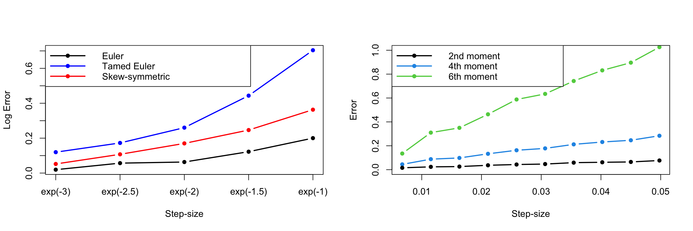
Figure 1: Figure on the left-hand side shows logarithm of the absolute error when computing $\mathbb{E}_{x}[Y_{T}^{2}]$ for $T$ fixed for the Ornstein–Uhlenbeck process. Figure on the right-hand side shows absolute error when computing moments of the density $\pi(x)\propto e^{-x^{4}/4}$ by simulating the overdamped Langevin diffusion over long time scales.

5.2 Poisson random effects model

Next we compare the performance of the Euler–Maruyama and skew-symmetric schemes for long-time simulation of an overdamped Langevin diffusion with equilibrium distribution corresponding to the posterior of a Poisson random effects model, which is popular in Bayesian Statistics (e.g. [DGM00, ZK91]). Using the Euler–Maruyama scheme equates to implementing the unadjusted Langevin algorithm (ULA) to sample from the associated posterior distribution. We compare the performance of ULA with the skew-symmetric scheme, with probability function $p$ chosen as in Example 2.1.1, which in this setting we call the unadjusted Barker algorithm (UBA).

The Poisson random effects model is of the following form:

$$\begin{split}y_{ij}|\eta_{i}&\sim\text{Poi}(e^{\eta_{i}}),\quad\quad j=1,\ldots,J,\\ \eta_{i}|\mu&\sim N(\mu,1),\quad\quad\,\,i=1,\ldots,I,\\ \mu&\sim N(0,\sigma_{\mu}^{2}).\end{split}$$

Defining the state vector $x=(\mu,\eta_{1},...,\eta_{I})$, this results in a posterior distribution with density $\pi(x)\propto\exp\{-U(x)\}$ and corresponding potential

$$U(x)=J\sum_{i}e^{\eta_{i}}-\sum_{i,j}y_{ij}\eta_{i}+\frac{1}{2}\sum_{i}(\eta_{i}-\mu)^{2}+\frac{\mu^{2}}{2\sigma^{2}_{\mu}}.$$

We approximate the resulting overdamped Langevin diffusion $\mathrm{d}X_{t}=-\nabla U(X_{t})\mathrm{d}t+\sqrt{2}\mathrm{d}W_{t}$, with a key focus on simulating from the distribution with density $\pi(x)\propto e^{-U(x)}$. Note that the drift vector is not globally Lipschitz.

The data $y_{ij}$ for $i=1,...,I$ and $j=1,...,J$ were simulated using true parameter values $\mu^{*}=5$, with each $\eta_{i}\sim N(\mu^{*},1)$. To generate the data we set $I=50$, $J=5$ and $\sigma_{\mu}=10$. With these choices there are enough observations that the marginal posterior distribution for $\mu$ is essentially centred at $\mu^{*}$. We compared the two numerical schemes by assessing the quality of ergodic averages of $\mu$ using mean squared Monte Carlo error for a fixed number of simulation steps. For each step-size $\Delta t$ we repeated the simulation 100 times and in each case evaluated the ergodic average of $\mu$. We then computed the empirical mean squared error of these estimates as compared to $\mu^{*}$. Larger step-sizes decrease the level of correlation between neighbouring iterates, reducing the Monte Carlo variance associated with ergodic averages, but increase the bias.

We consider two ways to initialise the scheme. The first is to initialise at the true value $\mu^{*}=5$. The second is to draw the starting point from a $\text{N}(5,10^{2})$ distribution, often called a warm start. In the latter case we expect the resulting Markov chain to have an initial transient phase before reaching equilibrium, so $10,000$ initial steps were discarded before another $50,000$ were used to evaluate mean squared error. The choice of $10,000$ iterations to discard was made using pilot runs and visual inspection of trajectories. We note in passing that ULA tended to take a longer time to reach equilibrium than UB for the same choice of step-size. In both settings each $\eta_{i}|\mu$ was initialised from the distribution $N(\mu,1)$.

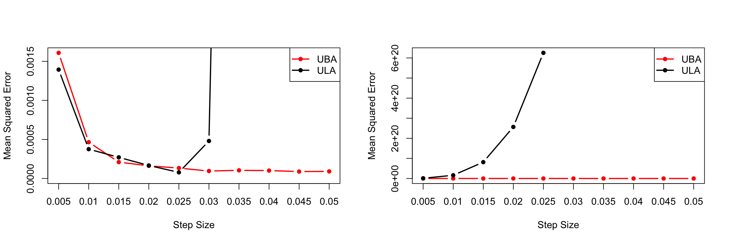
Figure 2: Mean squared error comparisons for the Poisson random effects example. Figure 2(a) (left-hand side) shows means squared error when initialised at the true value $\mu^{*}$. Figure 2(b) (right-hand side) is initialised from a $N(5,10^{2})$ sample.

As shown in Figure 2, when initialised at $\mu^{*}$ ULA performs poorly for $\Delta t\geq 0.03$, while UBA performs reasonably for all step-sizes used in the simulation. The two schemes perform similarly for small step sizes. The warm start results are more pronounced, as shown in Figure 2, as the UBA mean squared error never goes above 0.007 whereas the ULA error increases exponentially quickly as $\Delta t$ increases.

5.3 Soft spheres in an anharmonic trap

In this experiment we simulate particles in two spatial dimensions with soft sphere interactions evolving in an anharmonic trap (see e.g. Section 4.2 of [BVE23]). The particle dynamics are governed by the stochastic differential equation

$$\mathrm{d}X_{t}^{(i)}=\,\, 4B(\beta-X_{t}^{(i)})\|X_{t}^{(i)}-\beta\|^{2}\,\mathrm{d}t$$

$$+\frac{A}{Nr^{2}}\sum_{j=1}^{N}(X_{t}^{(i)}-X_{t}^{(j)})e^{-\|X_{t}^{(i)}-X_{t}^{(j)}\|^{2}/2r^{2}}\,\mathrm{d}t+\sqrt{2D}\,\mathrm{d}W_{t},$$

for $i=1,2,\ldots,N$ where $\beta$ is the position of the trap, $A>0$ is the strength of the repulsion between spheres with radius $r$, and $B>0$ is the strength of the trap. We set $\beta=(0,0)^{T}$, $D=0.25$, $A=30$, $r=0.15$ and $N=50$. We vary the strength of the trap through parameter $B$ to vary the degree of numerical difficulty associated with the problem.

We compared the skew-symmetric and Euler–Maruyama schemes with step-sizes $\Delta t\in\{0.1,0.2,0.3,\ldots,1\}$ and $B\in\{0.1,0.2,0.3,\ldots,1\}$. For each $(\Delta t,B)$-pair the dynamics were simulated for 10 steps, and this simulation was then repeated 100 times. The initial positions of the particles were independently drawn from a uniform distribution on $[-1,1]^{2}$. We then measured the probability of numerical explosion, meaning the position of one or more spheres reaching $\pm\infty$ (a number too large/small for the computer to record) during the simulation. The proportion of times such an explosion occurred for each chosen $(\Delta t,B)$-pair is shown in Figure 3.

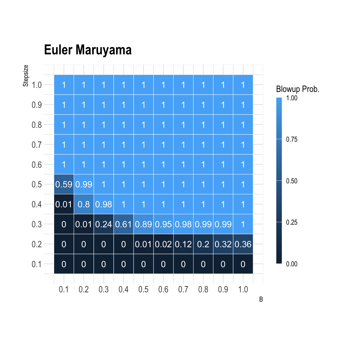
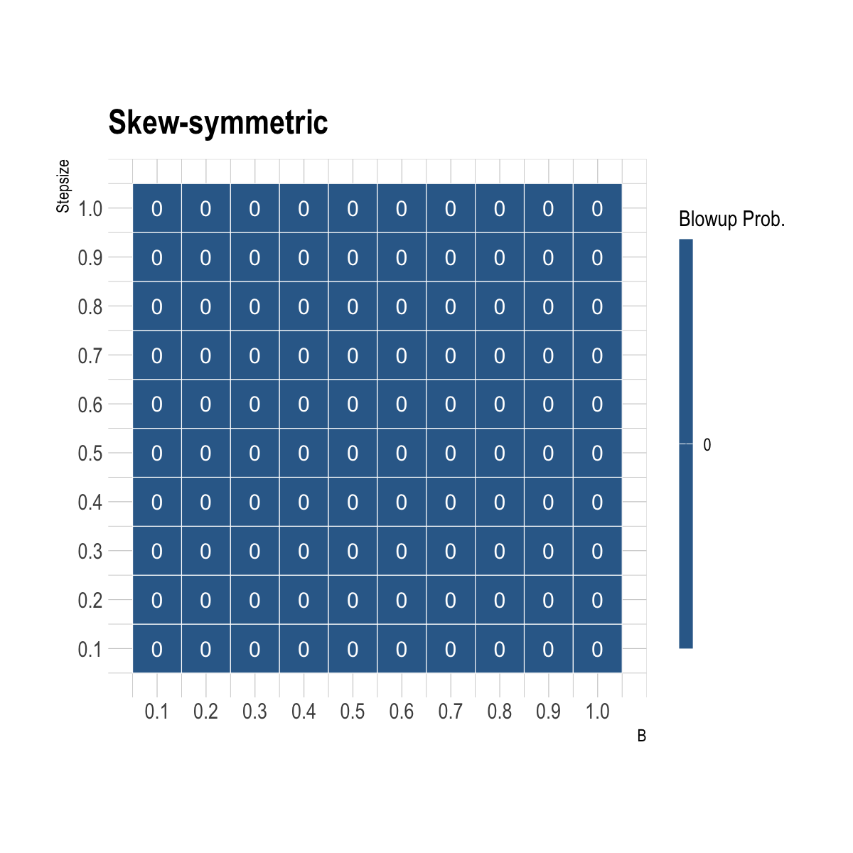
Figure 3: Heat map of numerical explosion probability for the soft spheres model. The $x$-axis shows chosen $B$ values, with larger $B$ increasing the level of difficulty of the problem, and the $y$ axis shows step-size.

The left-hand side of Figure 3 illustrates that explosion occurred for the Euler–Maruyama scheme quite frequently as either $B$ or $\Delta t$ increases. This is because the drift is not globally Lipschitz. The increase in $B$ implies a stronger attraction of the trap, which leads to more numerical difficulties and the need for a smaller step-size to ensure non-explosion on the simulation timescales. The skew-symmetric scheme is, however, extremely stable and does not exhibit any explosion events, as shown on the right-hand side of Figure 3.

6 Proof of Theorem 3.1

The proof proceeds by estimating the moments associated to (30) and its derivatives. We heavily rely on the theory of random diffeomorphisms induced by SDEs [Kun19], which in general requires global Lipschitz conditions. We circumvent this problem by taming the drift outside of a ball of large enough radius (see (51) below). We also note that, in order to shorten the notation, in the proof below the same letter $C$ will be used to denote potentially different upper bounding constants.

Proof of Theorem 3.1.

To ease notation, let us define $a(x):=\sigma(x)\sigma^{\top}(x)$, for $x\in\mathbb{R}^{d}$. By Lipschitz continuity of $\sigma$ (Assumption 2.2), $a$ grows at most quadratically,

$$\|a(x)\|_{F}\leq C(1+\|x\|^{2}),\qquad\qquad x\in\mathbb{R}^{d},$$ (43)

for an appropriate constant $C>0$. For $p\geq 2$, we will make repeated use of the derivatives

$$\frac{\partial\|A\|_{F}^{p}}{\partial A_{i_{1},\ldots,i_{n}}}=p\|A\|^{p-2}_{F}A_{i_{1},\ldots,i_{n}}$$ (44)

and

$$\frac{\partial^{2}\|A\|_{F}^{p}}{\partial A_{i_{1},\ldots,i_{n}}\partial A_{i^{\prime}_{1},\ldots,i^{\prime}_{n}}}= p\|A\|_{F}^{p-2}\delta_{(i_{1},\ldots,i_{n}),(i^{\prime}_{1},\ldots,i^{\prime}_{n})}$$ (45)

$$+p(p-2)\|A\|_{F}^{p-4}A_{i_{1},\ldots,i_{n}}A_{i_{1}^{\prime},\ldots,i_{n}^{\prime}},$$

where in (45), $\delta_{(i_{1},\ldots,i_{n}),(i^{\prime}_{1},\ldots,i^{\prime}_{n})}$ is equal to one if all indices coincide ($i_{1}=i^{\prime}_{1}$, $i_{2}=i^{\prime}_{2}$, …, $i_{n}=i^{\prime}_{n}$), and zero otherwise.

Estimates on $Y^{x}_{t}$. By Itô’s formula and (44)-(45), we have a.s.

$$\|Y^{x}_{t}\|^{p}= \|x\|^{p}+\int_{0}^{t}p\|Y^{x}_{s}\|^{p-2}Y^{x}_{s}\,\mu\left(Y^{x}_{s}\right)ds+\int_{0}^{t}\|Y^{x}_{s}\|^{p-2}Y^{x}_{s}\,\sigma\left(Y^{x}_{s}\right)dW_{s}$$

$$+\int_{0}^{t}\frac{1}{2}p\|Y^{x}_{s}\|^{p-2}\mathrm{Tr}\,a(Y^{x}_{s})\,\mathrm{d}s+\int_{0}^{t}\frac{1}{2}p(p-2)\|Y_{s}\|^{p-4}Y_{s}^{\top}a(Y^{x}_{s})Y^{x}_{s}\,\mathrm{d}s,$$ (46)

for all $t\in[0,T]$. In particular, if we introduce for any $R\in\mathbb{N}$ the stopping time

$$\tau_{R}=\inf\left\{t\geq 0:\ \|Y^{x}_{t}\|\geq R\right\},$$ (47)

and denote $t\wedge\tau_{R}=\min\{t,\tau_{R}\}$ we get a.s. for all $R\in\mathbb{N}$ and $t\in[0,T]$,

$$\|Y^{x}_{t\wedge\tau_{R}}\|^{p}=\|x\|^{p}+\int_{0}^{t\wedge\tau_{R}}p\|Y^{x}_{s}\|^{p-2}Y^{x}_{s}\,\mu\left(Y^{x}_{s}\right)ds+\int_{0}^{t\wedge\tau_{R}}\|Y^{x}_{s}\|^{p-2}Y^{x}_{s}\,\sigma\left(Y^{x}_{s}\right)dW_{s}$$

$$+\int_{0}^{t\wedge\tau_{R}}\frac{1}{2}p\|Y^{x}_{s}\|^{p-2}\mathrm{Tr}\,a(Y^{x}_{s})\,\mathrm{d}s+\int_{0}^{t\wedge\tau_{R}}\frac{1}{2}p(p-2)\|Y^{x}_{s}\|^{p-4}\left(Y_{s}^{x}\right)^{\top}a(Y^{x}_{s})Y^{x}_{s}\,\mathrm{d}s.$$

We observe that $\left(\int_{0}^{t\wedge\tau_{R}}\|Y^{x}_{s}\|^{p-2}Y^{x}_{s}\,\sigma\left(Y^{x}_{s}\right)dW_{s}\right)_{t\geq 0}$ is a true martingale, since the integrand is bounded, therefore it has zero expectation. Taking expectations, using the one-sided Lipschitz condition on $\mu$ (Assumption 2.1) as well as (43), and using Fubini’s theorem to exchange integral and expectation we see that there exists a constant $C>0$ such that

$$\mathbb{E}\left[\|Y^{x}_{t\wedge\tau_{R}}\|^{p}\right]\leq\|x\|^{p}+C\int_{0}^{t}\mathbb{E}[\|Y^{x}_{s\wedge\tau_{R}}\|^{p-2}]\,\mathrm{d}s+C\int_{0}^{t}\mathbb{E}[\|Y^{x}_{s\wedge\tau_{R}}\|^{p}]\,\mathrm{d}s,$$

for all $t\in[0,T]$. In particular,

$$\mathbb{E}\left[\|Y^{x}_{t\wedge\tau_{R}}\|^{p}\right] \leq\|x\|^{p}+C\int_{0}^{t}\mathbb{E}[\|Y^{x}_{s\wedge\tau_{R}}\|^{p}]+1\,\mathrm{d}s+C\int_{0}^{t}\mathbb{E}[\|Y^{x}_{s\wedge\tau_{R}}\|^{p}]\,\mathrm{d}s$$

$$\leq\|x\|^{p}+CT+2C\int_{0}^{t}\mathbb{E}[\|Y^{x}_{s\wedge\tau_{R}}\|^{p}]\,\mathrm{d}s.$$

Gronwall’s inequality then implies

$$\mathbb{E}[\|Y^{x}_{t\wedge\tau_{R}}\|^{p}]\leq C_{p}\left(\|x\|^{p}+1\right),\qquad x\in\mathbb{R}^{d},$$ (48)

for an appropriate constant $C_{p}>0$, independent of $t\in[0,T]$ and $R\in\mathbb{N}$. In particular, for any set $A\in\mathcal{B}(\mathbb{R}^{d})$, using Hölder’s inequality inequality for any $p^{\prime}>p$, we have that

$$\mathbb{E}[\|Y^{x}_{t\wedge\tau_{R}}\|^{p}1_{A}]\leq\mathbb{E}[\|Y^{x}_{t\wedge\tau_{R}}\|^{p^{\prime}}]^{1/p^{\prime}}\mathbb{P}\left(A\right)^{1-1/p^{\prime}}\leq C_{p^{\prime}}\left(\|x\|^{p^{\prime}}+1\right)\mathbb{P}\left(A\right)^{1-1/p^{\prime}}.$$

Consequently, the family of random variables $\left(\|Y^{x}_{t\wedge\tau_{R}}\|^{p}\right)_{R\in\mathbb{N}}$ is uniformly integrable in the sense of [BR07, Section 4.5]. Since a.s. $\lim_{R\rightarrow\infty}Y^{x}_{t\wedge\tau_{R}}=Y^{x}_{t}$, using Vitali’s theorem [BR07, Theorem 4.5.4] we get

$$\lim_{R\rightarrow\infty}\mathbb{E}[\|Y^{x}_{t\wedge\tau_{R}}\|^{p}]=\mathbb{E}[\|Y^{x}_{t}\|^{p}],$$

and using (48) we get

$$\mathbb{E}[\|Y^{x}_{t}\|^{p}]\leq C_{p}\left(\|x\|^{p}+1\right),\qquad x\in\mathbb{R}^{d}.$$ (49)

Together with $f\in C_{P}^{l}(\mathbb{R}^{d})$, the bound (32) follows.

Estimates on $\nabla_{x}Y^{x}_{t}$. In order to deal with the non-Lipschitz character of the drift $\mu$, we first establish results on the tamed version (51) below. For any cut-off radius $r\in\mathbb{N}$, we fix a drift $\mu^{(r)}\in C_{b}^{\infty}(\mathbb{R}^{d};\mathbb{R}^{d})$ so that $\mu^{(r)}(x)=\mu(x)$ if $\|x\|\leq r$, , and such that

$$\xi^{\top}\nabla\mu^{(r)}(x)\xi\leq C\|\xi\|^{2},\qquad\text{for all}\,x,\xi\in\mathbb{R}^{d},$$ (50)

with the same constant $C$ as in (29), independent of $r$ (the drifts $\mu^{(r)}$ can straightforwardly be obtained by modifying $\mu$ outside of $\{x\in\mathbb{R}^{d}:\|x\|\leq r\}$, in such a way that (29) is not violated). We consider the SDEs

$$\mathrm{d}Y^{x,(r)}_{t}=\mu^{(r)}(Y^{x,(r)}_{t})\,\mathrm{d}t+\sigma(Y^{x,(r)}_{t})\,\mathrm{d}W_{t},\qquad Y^{x,(r)}_{0}=x.$$ (51)

By [Kun19, Theorem 3.4.1], there exists a modification of $(Y^{x,(r)}_{t})_{t\in[0,T]}$ which is continuously differentiable with respect to the initial condition, for all $t\in[0,T]$. The derivative $\nabla_{x}Y_{t}^{x,(r)}\in\mathbb{R}^{d\times d}$ satisfies the SDEs

$$\mathrm{d}\partial_{j}Y^{x,(r)}_{t,i}=\sum_{l=1}^{d}\partial_{l}\mu^{(r)}_{i}(Y^{x,(r)}_{t})\partial_{j}Y^{(x,r)}_{t,l}\,\mathrm{d}t+\sum_{k=1}^{d}\sum_{l=1}^{d}\partial_{l}\sigma^{(r)}_{i,k}(Y^{x,(r)}_{t})\partial_{j}Y^{x,(r)}_{t,l}\,\mathrm{d}W_{t}^{k},$$ (52)

for all $i,j=1,\ldots,d$, with initial condition $\nabla_{x}Y^{x,(r)}_{0}=I_{d}$. Based on (44) and (45), using Itô’s formula we get

$$\mathrm{d}\|\nabla_{x}Y^{x,(r)}_{t}\|_{F}^{p} =p\,\|\nabla_{x}Y^{x,(r)}_{t}\|_{F}^{p-2}\sum_{i,j,l=1}^{d}\partial_{l}\mu_{i}(Y^{x,(r)}_{t})\partial_{j}Y_{t}^{l}\partial_{j}Y_{t}^{i}\ \mathrm{d}t$$

$$+\frac{p}{2}\|\nabla_{x}Y^{x,(r)}_{t}\|_{F}^{p-2}\sum_{i,j,k=1}^{d}\left(\sum_{l=1}^{d}\partial_{l}\sigma_{i,k}(Y_{t}^{x,(r)})\partial_{j}Y_{t,l}^{x,(r)}\right)^{2}\mathrm{d}t$$ (53a)

$$+\frac{p(p-2)}{2}\|\nabla_{x}Y^{x,(r)}_{t}\|_{F}^{p-4}\!\!$$ (53b)

$$\sum_{i,i^{\prime},j,j^{\prime},l,l^{\prime},k=1}^{d}\partial_{l}\sigma_{i,k}(Y^{x,(r)}_{t})\partial_{l^{\prime}}\sigma_{i^{\prime},k}(Y^{x,(r)}_{t})\partial_{j}Y^{x,(r)}_{t,l}\partial_{j^{\prime}}Y^{x,(r)}_{t,l^{\prime}}\partial_{j}Y^{x,(r)}_{t,i}\partial_{j^{\prime}}Y^{x,(r)}_{t,i^{\prime}}\!\!\ \mathrm{d}t$$

$$+p\,\|\nabla_{x}Y^{x,(r)}_{t}\|_{F}^{p-2}\sum_{k=1}^{d}\sum_{i,j,l=1}^{d}\partial_{l}\sigma_{i,k}(Y^{x,(r)}_{t})\partial_{j}Y_{t}^{l}\partial_{j}Y_{t}^{i}\ \mathrm{d}W^{k}_{t}.$$

We observe that $\|\nabla_{x}Y_{0}^{x,(r)}\|_{F}^{p}=d^{p/2}$. Furthermore, for any $t\in[0,T]$, we have the bound

$$\int_{0}^{t}\|\nabla_{x}Y^{x,(r)}_{s}\|_{F}^{p-2}\sum_{i,j,l=1}^{d}\partial_{l}\mu^{i}(Y^{x,(r)}_{s})\partial_{j}Y_{s}^{l}\partial_{j}Y_{s}^{i}\,\mathrm{d}s\leq C\int_{0}^{t}\|\nabla_{x}Y^{x,(r)}_{s}\|_{F}^{p}\,\mathrm{d}s,$$

using (50), and where $C>0$ does not depend on $x$, $r$ or $t$. By the boundedness of $\nabla\sigma$ (Assumption 3.1), we have a similar bound on the terms in (53a) and (53b). Taking expectations, using a similar argument as in the discussion below (6) (by introducing appropriate stopping times $\tau_{R}$) to argue that any integral term with respect to the Brownian motion will have zero expectation, and exchanging integral and expectation using Fubini, we obtain for all $R\in\mathbb{N}$

$$\mathbb{E}\left[\|\nabla_{x}Y^{x,(r)}_{t\wedge\tau_{R}}\|_{F}^{p}\right]\leq d^{p/2}+C(T)\int_{0}^{t}\mathbb{E}\left[\|\nabla_{x}Y^{x,(r)}_{s\wedge\tau_{R}}\|_{F}^{p}\right]\mathrm{d}s,$$ (54)

for all $t\in[0,T]$, where $C$ does not depend on $r,R\in\mathbb{N}$, $t\in[0,T]$ or $x\in\mathbb{R}^{d}$. By Gronwall’s Lemma, we get that $\mathbb{E}\left[\|\nabla_{x}Y^{x,(r)}_{t\wedge\tau_{R}}\|_{F}^{p}\right]$ is bounded uniformly in $r,R\in\mathbb{N}$, $t\in[0,T]$ and $x\in\mathbb{R}^{d}$. Therefore, letting $R\rightarrow\infty$ and using Vitali’s theorem, we conclude that $\mathbb{E}\left[\|\nabla_{x}Y^{x,(r)}_{t}\|_{F}^{p}\right]$ is bounded uniformly in $r\in\mathbb{N}$, $t\in[0,T]$ and $x\in\mathbb{R}^{d}$.

Controlling the gradient of the cut-off semigroup. Defining the cut-off version of $u_{t}$,

$$u_{t}^{(r)}(x):=\mathbb{E}[f(Y_{t}^{x,(r)})],\qquad x\in\mathbb{R}^{d},$$ (55)

we next argue that $u_{t}^{(r)}$ is differentiable, with

$$\nabla_{x}u_{t}^{(r)}(x)=\mathbb{E}\left[\nabla_{x}Y_{t}^{x,(r)}\nabla f(Y^{x,(r)}_{t})\right],$$ (56)

that is, we can apply the gradient operation to (55) and exchange expectation and derivatives. To that end, notice that $x\mapsto f(Y_{t}^{x,(r)})$ is differentiable almost surely, with derivative $\nabla_{x}Y_{t}^{x,(r)}\nabla f(Y_{t}^{x,(r)})$. For fixed $x\in\mathbb{R}^{d}$, choose a bounded and open neighbourhood $\mathcal{U}_{x}\subset\mathbb{R}^{d}$. We observe that the argument establishing (49) works for the process $Y^{y,(r)}$ for any $y\in U_{x}$ and $r>0$, and the moment bound of (49) is independent of $r$. Combining this with the uniform bound on $\|\nabla_{y}Y_{t}^{y,(r)}\|_{F}^{p}$ from above, as well as the fact that $f\in C_{P}^{l}(\mathbb{R}^{d})$, we see that

$$\mathbb{E}\left[\|\nabla_{y}Y_{t}^{y,(r)}\nabla f(Y_{t}^{y,(r)})\|^{2}\right] \leq\left(\mathbb{E}[\|\nabla_{y}Y_{t}^{y,(r)}\|_{F}^{4}]\right)^{1/2}\left(\mathbb{E}[\|\nabla f(Y_{t}^{y,(r)})\|^{4}]\right)^{1/2}$$

$$\leq C(1+\|y\|^{m}),$$ (57a)

for appropriate constants $C>0$ and $m\in\mathbb{N}$, independent of $r$. Consequently the family of random variables $(\nabla_{y}Y_{t}^{(r)}\nabla f(Y_{t}^{(r)}))_{y\in\mathcal{U}_{x}}$ is uniformly integrable. Therefore, combining Vitali’s theorem with the proof technique from [BR07, Corollary 2.8.7(ii)], we can exchange differentiation and integration: Indeed, since $x\mapsto f(Y_{t}^{x,(r)})$ is continuously differentiable [Kun19, Theorem 3.4.1], the mean-value theorem allows us to choose (random) $\xi_{h,v}\in\mathbb{R}^{d}$ so that

$$\tfrac{1}{h}\left(f(Y_{t}^{x+hv,(r)})-f(Y_{t}^{x,(r)})\right)=v\cdot\nabla_{x}Y_{t}^{\xi_{h,v},(r)}\nabla f(Y_{t}^{\xi_{h,v},(r)}),$$ (58)

for all $h>0$ and $v\in\mathbb{R}^{d}$ such that $x+hv\in\mathcal{U}_{x}$. According to Vitali’s theorem, we can then pass this expression to the limit and exchange differentiation and integration. This proves (56). We also observe that a similar use of Vitali’s theorem shows that $\nabla_{x}u_{t}^{(r)}\in C(U;\mathbb{R}^{d})$.

Letting $r\rightarrow\infty$. To remove the cut-off, we show that for any open and bounded set $\mathcal{U}\subset\mathbb{R}^{d}$ and fixed $t\in[0,T]$, the sequence $(u_{t}^{(r)})_{r\in\mathbb{N}}$ converges uniformly to $u_{t}$ on $\mathcal{U}$, and likewise $(\nabla_{x}u^{(r)}_{t})_{r\in\mathbb{N}}$ is a Cauchy sequence in $C(\mathcal{U};\mathbb{R}^{d})$. Together, these claims show that $u_{t}$ is differentiable on $\mathcal{U}$, and the derivative coincides with the limit of $(\nabla_{x}u^{(r)}_{t})_{r\in\mathbb{N}}$. Furthermore, since the upper bound on (57) does not depend on $r$, we obtain the bound (33) for the limit $\nabla u_{t}$.

To show that $u_{t}^{(r)}\rightarrow u_{t}$, uniformly on $\mathcal{U}$, notice that

$$\sup_{x\in\mathcal{U}}|u_{t}^{(r)}(x)-u_{t}(x)|=\sup_{x\in\mathcal{U}}\left|\mathbb{E}\left[\left(f(Y_{t}^{x,(r)})-f(Y^{x}_{t})\right)\mathbb{I}\left(\sup_{0\leq s\leq t}\|Y^{x}_{t}\|\geq r\right)\right]\right|,$$ (59)

based on the fact that $Y_{t}^{(r)}$ and ${Y_{t}}$ can be coupled to coincide almost surely on ${\{\sup_{0\leq s\leq t}\|Y^{x}_{s}\|\leq r\}}$. Using Markov’s inequality, the fact that $f\in C_{P}^{l}(\mathbb{R}^{d})$ and the bound (49), we see that up to a multiplicative constant, this expression can be bounded by the supremum over $x\in U$ of the quantity

$$\frac{1}{r}\mathbb{E}\left[\sup_{0\leq s\leq t}\|Y^{x}_{s}\|\right]\leq\frac{1}{r}\mathbb{E}\left[\|x\|+\int_{0}^{t}\|\mu(Y_{s}^{x})\|\mathrm{d}s+\sup_{0\leq s\leq t}\left\|\int_{0}^{s}\sigma(Y_{s^{\prime}}^{x})\,\mathrm{d}W_{s^{\prime}}\right\|\right].$$ (60)

According to the Burkholder-Davis-Gundy (and using the polynomial growth assumption on $\mu$ and $\sigma$), this expression indeed converges to zero as $r\rightarrow\infty$, uniformly in $x\in\mathcal{U}$.

To show that $(\nabla_{x}u^{(r)}_{t})_{r\in\mathbb{N}}$ is a Cauchy sequence in $C(\mathcal{U};\mathbb{R}^{d})$, we observe that for any $r,\widetilde{r}>0$

$$\left\|\nabla_{x}u^{(r)}_{t}(x)-\nabla_{x}u^{(r+\widetilde{r})}_{t}(x)\right\|=\left\|\mathbb{E}\left[\nabla_{x}Y_{t}^{x,(r)}\nabla f(Y_{t}^{x,(r)})-\nabla_{x}Y_{t}^{x,(r+\widetilde{r})}\nabla f(Y_{t}^{x,(r+\widetilde{r})})\right]\right\|$$

$$= \left\|\mathbb{E}\left[\left(\nabla_{x}Y_{t}^{x,(r)}\nabla f(Y_{t}^{x,(r)})-\nabla_{x}Y_{t}^{x,(r+\widetilde{r})}\nabla f(Y_{t}^{x,(r+\widetilde{r})})\right)\mathbb{I}\left({\sup_{0\leq s\leq t}\|Y_{t}^{x,(r)}\|\geq r}\right)\right]\right\|,$$

Proceeding as above, and on letting $r\rightarrow\infty$, we get that $(\nabla_{x}u^{(r)}_{t})_{r\in\mathbb{N}}$ is a Cauchy sequence in $C(\mathcal{U};\mathbb{R}^{d})$.

Estimates on $\nabla^{n}Y^{x}_{t}$. To establish bounds on the higher-order derivatives, we proceed as before and consider the tamed SDE (51). Exchanging derivatives and expectations as well as removal of the cut-off $r\in\mathbb{N}$ works in the same way as for the first-order case. We therefore omit these details and lay out the main steps to establish bounds on moments of $\nabla_{x}^{n}Y_{t}^{x}$.

Before we write the SDE that is satisfied by $\nabla_{x}^{n}Y_{t}^{x,(r)}$ for $n\geq 2$, we need to introduce the following notation: For $k\in\mathbb{N}$ and for the vectors $\zeta^{1},...,\zeta^{k}\in\mathbb{R}^{d}$, we write

$$\nabla^{k}\mu_{i}(x)\left[\zeta^{1},...,\zeta^{k}\right]:=\sum_{j_{1},\dots,j_{k}=1}^{d}\partial_{j_{1}}\partial_{j_{2}}\dots\partial_{j_{k}}\mu_{i}(x)\zeta^{1}_{j_{1}}\zeta^{2}_{j_{2}}\dots\zeta^{k}_{j_{k}}.$$

Fix a set of indices $\left\{i_{1},...,i_{n}\right\}\subset\left\{1,...,d\right\}$. For any set $B=\left\{j_{1},...,j_{m}\right\}\subset\left\{i_{1},...,i_{n}\right\}$ we write $\nabla^{B}Y_{t}^{x,(r)}$ to denote the $d$-dimensional vector with $i$-coordinate given by

$$\nabla^{B}Y_{t,i}^{x,(r)}=\partial_{j_{1}}\dots\partial_{j_{m}}Y_{t,i}^{x,(r)}.$$

Now, let $\mathcal{A}^{k}_{i_{1},\dots,i_{n}}$ be the set of all possible partitions of set $\{i_{1},\dots,i_{n}\}$ that are composed of $k$ subsets of $\{i_{1},\dots,i_{n}\}$. For any such partition $A=\left\{A_{1},\dots,A_{k}\right\}\in\mathcal{A}^{k}_{i_{1},\dots,i_{n}}$ we write

$$\nabla^{k}\mu_{i}(x)\left[Y_{t}^{x,(r)},A\right]:=\nabla^{k}\mu_{i}(x)\left[\nabla^{A_{1}}Y_{t}^{x,(r)},\dots,\nabla^{A_{k}}Y_{t}^{x,(r)}\right].$$

Then, using an induction argument for $n\in\mathbb{N}$, along with [Kun19, Theorem 3.4.1] and straightforward calculations, one can conclude the following. For $n\geq 2$, the SDE that $\nabla_{x}^{n}Y_{t}^{x,(r)}$ satisfies is such that for any $i,i_{1},\dots,i_{n}\in\left\{1,\dots,d\right\}$, the drift of $\partial_{i_{1}}\dots\partial_{i_{n}}Y_{t,i}^{x,(r)}$ is given by

$$\nabla^{1}\mu_{i}(Y_{t}^{x,(r)})\left[\nabla^{i_{1},...,i_{n}}Y_{t}^{x,(r)}\right]+\sum_{k=2}^{n}\sum_{A\subset\mathcal{A}^{k}_{i_{1},\dots,i_{n}}}\!\!\!\nabla^{k}\mu_{i}(Y_{t}^{x,(r)})\left[Y_{t}^{x,(r)},A\right]\mathrm{d}t,$$ (62)

and the volatility is given by

$$\sum_{j=1}^{d}\nabla^{1}\sigma_{i,j}(Y_{t}^{x,(r)})\left[\nabla^{i_{1},...,i_{n}}Y_{t}^{x,(r)}\right]+\sum_{k=2}^{n}\sum_{A\subset\mathcal{A}^{k}_{i_{1},\dots,i_{n}}}\!\!\nabla^{k}\sigma_{i,j}(Y_{t}^{x,(r)})\left[Y_{t}^{x,(r)},A\right]\mathrm{d}W^{j}_{t}.$$ (63)

with initial conditions $\nabla^{n}_{x}Y^{x,(r)}_{0}=0$. We observe that the only terms that involve $n$’th order derivatives of $Y_{t}^{x,(r)}$ appear on the first term of (62) and (63), with coefficients $\nabla\mu_{i}$ and $\nabla\sigma_{i,j}$ respectively. All the other terms involve lower order derivatives.

In complete analogy with (53), we apply Itô’s formula to obtain an evolution equation for $\mathbb{E}[\|\nabla^{n}_{x}Y^{x,(r)}_{t}\|^{p}]$. The only terms in the Itô expansion that will involve the quantity $\|\nabla^{n}_{x}Y^{x,(r)}_{t}\|^{p}$ come from the first terms of (62) and (63), and these can be bounded in the same way as for $n=1$ (see the inequality below (53b)), making essential use of (29) and the boundedness of $\nabla\sigma$. All the other terms in the Itô expansion, correspond to products between $\|\nabla^{n}_{x}Y^{x,(r)}_{t}\|^{q}$ for various $q<p$ and lower order derivatives of $Y^{x,(r)}_{t}$. The expectations of these contributions can be bounded inductively: First we use Hölder’s inequality to bound the expectation of such product by the product between the expectation of $\|\nabla^{n}_{x}Y^{x,(r)}_{t}\|^{p}$ (raised to the power $\frac{q}{p}<1$) and a moment of lower order derivatives. These moments have been shown to be bounded uniformly in $r$ and $t$ in the previous steps, where we consider lower order derivatives. Finally, any moment of $\nabla^{k}\sigma(Y_{t}^{x,(r)})$ or $\nabla^{k}\mu(Y_{t}^{x,(r)})$ for any $k=0,...,n$ can be bounded using boundedness of derivatives of $\sigma$ and the polynomial bounds on derivatives of $\mu$, in conjuction with the the bound on the the moments of $Y_{t}^{x}$ established in (49). This shows the uniform bound (over $t,r$) of all moments of $n$’th order derivatives, given the bounds for order $k=0,...,n-1$.

∎

7 Conclusion

We have introduced a new simple and explicit numerical scheme for time-homogeneous and uniformly elliptic stochastic differential equations. The skew-symmetric scheme updates its current position using a two-step process: for each coordinate, first the size of the jump is simulated without the influence of the drift, and then the direction of the jump is decided, based on a probability that depends on both the drift and volatility of the current position. This mechanism makes the scheme highly robust when the drift is not globally Lipschitz. We have established basic results on the weak convergence of the numerical scheme, and, while proving these, we generalised the theory of Milstein and Tretyakov [MT21, Theorem 2.2.1] to non-globally Lipschitz drifts. Strong convergence results are left as an open question.

A key concern of the article is long-time simulation of ergodic diffusions. To this end, we have established that the skew-symmetric scheme can be used to generate approximate samples from the invariant distribution of such a diffusion. Under suitable conditions we have established that the numerical scheme converges at a geometric rate to its equilibrium distribution. We have also provided quantitative bounds on the distance between the equilibria of the numerical and exact processes with respect to the numerical step-size. Finally, we performed experiments in Section 5, providing empirical evidence to support our theoretical results.

Funding

SL and GV were supported by an EPSRC New Investigator Award (EP/V055380/1). RZ was supported by an LMS undergraduate bursary (URB-2023-71).

Appendix A Proof of Proposition 3.1

We begin with the following simple observation.

Lemma A.1.

If we write $b=(b_{1},...,b_{d})\in\{\pm 1\}^{d}$, then for any $n\in\mathbb{N}$ and $i_{1},...,i_{n}\in\{1,...,d\}$, the following statements hold. If at least one of the $i_{j}$’s appears an odd number of times amongst $\{i_{1},...,i_{n}\}$ then

$$\sum_{b\in\{\pm 1\}^{d}}b_{i_{1}}b_{i_{2}}...b_{i_{n}}=0.$$

Otherwise

$$\sum_{b\in\{\pm 1\}^{d}}b_{i_{1}}b_{i_{2}}...b_{i_{n}}=2^{d}.$$

Proof of Lemma A.1.

Assume first that at least one of the coordinates (assume without loss of generality that this is $i_{n}$) appears an odd number of times amongst $i_{1},...,i_{n}$. Then, there exist $k\in\mathbb{N}$ and $j_{1},j_{2},...,j_{m}\neq i_{n}$ such that

$$\sum_{b\in\{\pm 1\}^{d}}b_{i_{1}}...b_{i_{n}}=\sum_{b\in\{\pm 1\}^{d}}b_{j_{1}}...b_{j_{m}}b^{2k+1}_{i_{n}}$$

$$=2^{d-m-1}\sum_{b_{j_{1}},b_{j_{2}},...b_{j_{m}}\in\{\pm 1\}}\sum_{b_{i_{n}}\in\{\pm 1\}}b_{j_{1}}...b_{j_{m}}b_{i_{n}}$$

$$=2^{d-m-1}\sum_{b_{j_{1}},b_{j_{2}},...b_{j_{m}}\in\{\pm 1\}}b_{j_{1}}...b_{j_{m}}\sum_{b_{i_{n}}\in\{\pm 1\}}b_{i_{n}}=0.$$

If, on the other hand, every $i_{j}$ appears an even number of times amongst $i_{1},...,i_{d}$, then, since $b_{i_{j}}\in\{\pm 1\}$, the product between the even number of terms that are $b_{i_{j}}$ is equal to one. Therefore

$$\sum_{b\in\{\pm 1\}^{d}}b_{i_{1}}...b_{i_{n}}=\sum_{b\in\{\pm 1\}^{d}}1=2^{d}.$$

∎

We also use the following well-known result for moments of multivariate Gaussians. This is the odd-dimensional version of Isserlis’ theorem, (see e.g. [FV17, Chapter 8: Exercise 8.3]).

Theorem A.1 (Isserlis’ Theorem).

If $Y=(Y_{1},...,Y_{d})$ is a $d$-dimensional Gaussian, with $d$ odd then

$$\mathbb{E}\left[Y_{1}Y_{2}\ldots Y_{d}\right]=0.$$

We can now prove Proposition 3.1.

Proof of Proposition 3.1.

We only prove the second part of the proposition. The first part follows using a similar argument.

Recall that after one step, the process starting from $x\in\mathbb{R}^{d}$ will transition to $X_{1}=x+\xi\ast b$, where for all $i\in\{1,...,d\}$, $\xi_{i}=\sqrt{\Delta t}\sigma_{i,i}(x)\nu_{i}$, $\nu\sim N(0,I_{d})$ and $b_{i}=+1$ with probability $q_{i}(x,\xi)$ or $b_{i}=-1$ with probability $1-q_{i}(x,\xi)$. Recall that for two vectors $u,v\in\mathbb{R}^{d}$, we write $u\ast v\in\mathbb{R}^{d}$ to denote the vector of element-wise products between $c$ and $d$. Then we can write

$$\mathbb{E}_{x}\left[f(X_{1})-f(x)\right]=\sum_{b\in\{\pm 1\}^{d}}\mathbb{E}_{\nu}\Bigg{[} \left(f(x+\sqrt{\Delta t}(\sigma(x)\nu)\ast b)-f(x)\right)\cdot$$ (64)

$$\cdot\prod_{i=1}^{d}\left[q_{i}(x,\xi)\mathbb{I}(b_{i}=1)+(1-q_{i}(x,\xi))\mathbb{I}(b_{i}=-1)\right]\Bigg{]}.$$

Let us introduce the following notation. For any $n\in\mathbb{N}$, and any vector $w=(w_{1},...,w_{d})\in\mathbb{R}^{d}$, we write

$$f^{(n)}(y)\left(w\right)^{n}=\sum_{i_{1},...,i_{n}\in\{1,...,d\}}\partial^{y}_{i_{1}}\partial^{y}_{i_{2}}...\partial^{y}_{i_{n}}f(y)w_{i_{1}}w_{i_{2}}...w_{i_{n}}.$$

Then, a Taylor expansion with respect to $\Delta t^{1/2}$ around $0$ gives

$$f(x+\sqrt{\Delta t}(\sigma(x)\nu)\ast b)-f(x)$$ (65)

$$=\Delta t^{1/2}f^{(1)}(x)((\sigma(x)\nu)\ast b)^{1}+\frac{1}{2}\Delta t^{2/2}f^{(2)}(x)((\sigma(x)\nu)\ast b)^{2}$$

$$+\frac{1}{3!}\Delta t^{3/2}f^{(3)}(x)((\sigma(x)\nu)\ast b)^{3}+\frac{1}{4!}\Delta t^{4/2}f^{(4)}(x)((\sigma(x)\nu)\ast b)^{4}$$

$$+\frac{1}{5!}\Delta t^{5/2}f^{(5)}(x)((\sigma(x)\nu)\ast b)^{5}+\frac{1}{6!}\Delta t^{6/2}f^{(6)}(x+\tau_{1}(\sigma(x)\nu)\ast b)((\sigma(x)\nu)\ast b)^{6},$$

for some $\tau_{1}\in(0,\Delta t^{1/2})$, and another Taylor expansion of $q_{i}(x,\xi)$ with respect to $\xi=\Delta t^{1/2}\sigma(x)\nu$ around $0$ gives

$$q_{i}(x,\xi)= q_{i}(x,0)\!+\!\Delta t^{1/2}q_{i}^{(1)}(x,0)(\sigma(x)\nu)^{1}\!+\!\frac{1}{2}\Delta t^{2/2}q_{i}^{(2)}(x,0)(\sigma(x)\nu)^{2}\!$$

$$\!+\frac{1}{3!}\Delta t^{3/2}q_{i}^{(3)}(x,0)(\sigma(x)\nu)^{3}+\!\frac{1}{4!}\!\Delta t^{4/2}q_{i}^{(4)}(x,0)(\sigma(x)\nu)^{4}\!$$

$$\!+\frac{1}{5!}\Delta t^{5/2}q_{i}^{(5)}(x,0)(\sigma(x)\nu)^{5}\!+\!\frac{1}{6!}\Delta t^{6/2}q_{i}^{(6)}(x,\tau_{2}\sigma(x)\nu)(\sigma(x)\nu)^{6},$$

for some $\tau_{2}\in(0,\Delta t^{1/2})$, where all the derivatives for $q_{i}(x,\xi)$ are taken with respect to $\xi$. Noting that $q_{i}(x,0)=\frac{1}{2}$, we see that

$$q_{i}(x,\xi)\mathbb{I}(b_{i}=1)+\left(1-q_{i}(x,\xi)\right)\mathbb{I}(b_{i}=-1)$$

$$=\frac{1}{2}+b_{i}\Delta t^{1/2}q_{i}^{(1)}(x,0)(\sigma(x)\nu)^{1}+b_{i}\frac{1}{2}\Delta t^{2/2}q_{i}^{(2)}(x,0)(\sigma(x)\nu)^{2}$$ (66)

$$+b_{i}\frac{1}{3!}\Delta t^{3/2}q_{i}^{(3)}(x,0)(\sigma(x)\nu)^{3}+b_{i}\frac{1}{4!}\Delta t^{4/2}q_{i}^{(4)}(x,0)(\sigma(x)\nu)^{4}$$

$$+b_{i}\frac{1}{5!}\Delta t^{5/2}q_{i}^{(5)}(x,0)(\sigma(x)\nu)^{5}+b_{i}\frac{1}{6!}\Delta t^{6/2}q_{i}^{(6)}(x,\tau_{2}\sigma(x)\nu)(\sigma(x)\nu)^{6}$$

Combining (65) and (A) we view the product inside the expectation of $(\ref{semigroup.expansion.product:1})$ as a polynomial in $\Delta t^{1/2}$, up to an error term. We will now identify the coefficients of this polynomial. First of all, we consider the coefficient of the term $\Delta t^{1/2}$. This is

$$f^{(1)}(x)((\sigma(x)\nu)\ast b)^{1}\left(\frac{1}{2}\right)^{d}=\left(\frac{1}{2}\right)^{d}\sum_{i=1}^{d}\partial_{i}f(x)\sigma_{i,i}(x)\nu_{i}b_{i}.$$

Taking the expectation over $\nu$, we see that this is equal to zero, since $\sigma(x)\nu\sim N(0,\sigma\sigma^{T})$.

Next, we consider the coefficient of $\Delta t$. Considering the different ways in which the $d+1$ factors in (64) can give order $\Delta t$ though the Taylor expansions (65) and (A), we see that the coefficient is

$$f^{(1)}(x)((\sigma(x)\nu)\ast b)^{1} \sum_{k=1}^{d}b_{k}q_{k}^{(1)}(x,0)(\sigma(x)\nu)^{1}\left(\frac{1}{2}\right)^{d-1}$$ (67)

$$+\frac{1}{2!}f^{(2)}(x)((\sigma(x)\nu)\ast b)^{2}\left(\frac{1}{2}\right)^{d}$$

Let’s consider each part of the sum separately. We write

$$f^{(1)}(x)((\sigma(x)\nu)\ast b)^{1}\sum_{k=1}^{d}b_{k}q_{k}^{(1)}(x,0)(\sigma(x)\nu)^{1}\left(\frac{1}{2}\right)^{d-1}$$

$$=\left(\frac{1}{2}\right)^{d-1}\sum_{i,j,k=1}^{d}\partial_{i}f(x)b_{i}\sigma_{i,i}(x)\nu_{i}b_{k}\partial^{\xi}_{j}q_{k}(x,0)\sigma_{j,j}(x)\nu_{j}$$

Summing over $b\in\{\pm 1\}^{d}$ to obtain (64), we get

$$\left(\frac{1}{2}\right)^{d-1}\sum_{i,j,k=1}^{d}\partial_{i}f(x)\sigma_{i,i}(x)\nu_{i}\partial^{\xi}_{j}q_{k}(x,0)\sigma_{j,j}(x)\nu_{j}\sum_{b\in\{\pm 1\}^{d}}b_{i}b_{k}.$$ (68)

From Lemma A.1 we have

$$\sum_{b\in\{\pm 1\}^{d}}b_{i}b_{k}=2^{d}\mathbb{I}(i=k),$$ (69)

therefore (68) gives

$$2\sum_{i,j=1}^{d}\partial_{i}f(x)\partial^{\xi}_{j}q_{i}(x,0)\sigma_{i,i}(x)\nu_{i}\sigma_{j,j}(x)\nu_{j}.$$

Taking the expectation over $\nu\sim N(0,I_{d})$ and using (23), we see that

$$\mathbb{E}\left[2\sum_{i,j=1}^{d}\partial_{i}f(x)\partial^{\xi}_{j}q_{i}(x,0)\sigma_{i,i}(x)\nu_{i}\sigma_{j,j}(x)\nu_{j}\right]=\sum_{i=1}^{d}\partial_{i}f(x)2\partial^{\xi}_{i}q_{i}(x,0)\sigma_{i,i}^{2}(x)$$ (70)

$$=\sum_{i=1}^{d}\partial_{i}f(x)\mu_{i}(x)=\mu(x)\cdot\nabla f(x).$$

For the other part of the sum in (67) we have

$$\left(\frac{1}{2}\right)^{d}\frac{1}{2!}f^{(2)}(x)((\sigma(x)\nu)\ast b)^{2}=\frac{1}{2^{d+1}}\sum_{i,j=1}^{d}\partial_{i}\partial_{j}f(x)b_{i}\sigma_{i,i}(x)\nu_{i}b_{j}\sigma_{j,j}(x)\nu_{j}.$$

Summing over $b\in\{\pm 1\}^{d}$, we get

$$\frac{1}{2^{d+1}}\sum_{i,j=1}^{d}\partial_{i}\partial_{j}f(x)\sigma_{i,i}(x)\nu_{i}\sigma_{j,j}(x)\nu_{j}\sum_{b\in\{\pm 1\}^{d}}b_{i}b_{j},$$

and using (69) this is equal to

$$\frac{2^{d}}{2^{d+1}}\sum_{i=1}^{d}\partial_{i}^{2}f(x)\sigma_{i,i}^{2}(x)\nu_{i}^{2},$$

the expectation of which is

$$\frac{1}{2}\sum_{i=1}^{d}\partial_{i}^{2}f(x)\sigma_{i,i}^{2}(x).$$ (71)

Combining this with (70), and in view of Assumption 2.2.2, we see that the coefficient of $\Delta t$ is $Lf(x)$, where $L$ as in (25) is the generator of the diffusion we are approximating.

We now consider the coefficient of the term $\Delta t^{3/2}$. Considering the different ways in which the $d+1$ factors in (64) can give order $\Delta t^{3/2}$ through the Taylor expansions (65) and (A), we see that the coefficient is

$$f^{(1)}(x)((\sigma(x)\nu)\ast b)^{1}\sum_{i=1}^{d}\frac{1}{2!}b_{i}q_{i}^{(2)}(x,0)(\sigma(x)\nu)^{2}\left(\frac{1}{2}\right)^{d-1}$$

$$+f^{(1)}(x)((\sigma(x)\nu)\ast b)^{1}\sum_{i\neq j}b_{i}q_{i}^{(1)}(x,0)(\sigma(x)\nu)^{1}b_{j}q_{j}^{(1)}(x,0)(\sigma(x)\nu)^{1}\left(\frac{1}{2}\right)^{d-2}$$

$$+\frac{1}{2!}f^{(2)}(x)((\sigma(x)\nu)\ast b)^{2}\sum_{i=1}^{d}b_{i}q_{i}(x,0)(\sigma(x)\nu)^{1}\left(\frac{1}{2}\right)^{d-1}$$

$$+\frac{1}{3!}f^{(3)}(x)((\sigma(x)\nu)\ast b)^{3}\left(\frac{1}{2}\right)^{d}.$$

Taking expectations over $\nu$, all four summands involve terms of the form $\mathbb{E}_{\nu}\left[\nu_{i_{1}}\nu_{i_{2}}\nu_{i_{3}}\right]$, for $i_{1},i_{2},i_{3}\in\{1,2,...,d\}$. From Theorem A.1, since $\nu\sim N(0,I_{d})$, these expectations are zero, so the coefficient of $\Delta t^{3/2}$ is zero.

Using a similar argument, we can also conclude that the coefficient of the term $\Delta t^{5/2}$ is zero as well.

We now consider the coefficient of the term $\Delta t^{2}$. Considering the different ways in which the $d+1$ factors in (64) can give order $\Delta t^{4/2}$ through the Taylor expansions (65) and (A), we see that the coefficient is

$$f^{(1)}(x)((\sigma(x)\nu)\ast b)^{1}\sum_{i=1}^{d} \frac{1}{3!}b_{i}q_{i}^{(3)}(x,0)(\sigma(x)\nu)^{3}\left(\frac{1}{2}\right)^{d-1}$$ (72)

$$+f^{(1)}(x)((\sigma(x)\nu)\ast b)^{1}\sum_{i\neq j} \frac{1}{2!}b_{i}q_{i}^{(2)}(x,0)(\sigma(x)\nu)^{2}b_{j}q_{j}^{(1)}(x,0)(\sigma(x)\nu)^{1}\left(\frac{1}{2}\right)^{d-2}$$

$$+f^{(1)}(x)((\sigma(x)\nu)\ast b)^{1}\sum_{i\neq j\neq k\neq i} b_{i}q_{i}^{(1)}(x,0)(\sigma(x)\nu)^{1}b_{j}q_{j}^{(1)}(x,0)(\sigma(x)\nu)^{1}$$

$$b_{k}q_{k}^{(1)}(x,0)(\sigma(x)\nu)^{1}\left(\frac{1}{2}\right)^{d-3}$$

$$+\frac{1}{2!}f^{(2)}(x)((\sigma(x)\nu)\ast b)^{2}\sum_{i=1}^{d} \frac{1}{2!}b_{i}q_{i}^{(2)}(x,0)(\sigma(x)\nu)^{2}\left(\frac{1}{2}\right)^{d-1}$$

$$+\frac{1}{2!}f^{(2)}(x)((\sigma(x)\nu)\ast b)^{2}\sum_{i\neq j} b_{i}q_{i}^{(1)}(x,0)(\sigma(x)\nu)^{1}b_{j}q_{j}^{(1)}(x,0)(\sigma(x)\nu)^{1}\left(\frac{1}{2}\right)^{d-2}$$

$$+\frac{1}{3!}f^{(3)}(x)((\sigma(x)\nu)\ast b)^{3}\sum_{i=1}^{d} b_{i}q_{i}^{(1)}(x,0)(\sigma(x)\nu)\left(\frac{1}{2}\right)^{d-1}$$

$$+\frac{1}{4!}f^{(4)}(x)((\sigma(x)\nu)\ast b)^{4}\left(\frac{1}{2}\right)^{d}.$$

Let us consider each of those 7 terms separately. For the first term, we write

$$f^{(1)}(x)((\sigma(x)\nu)\ast b)^{1}\sum_{i=1}^{d}\frac{1}{3!}b_{i}q_{i}^{(3)}(x,0)(\sigma(x)\nu)^{3}\left(\frac{1}{2}\right)^{d-1}$$

$$=\frac{1}{3!2^{d-1}}\sum_{i,k,i_{1},i_{2},i_{3}=1}^{d}\partial_{k}f(x)b_{k}\sigma_{k,k}(x)\nu_{k}b_{i}\partial^{\xi}_{i_{1}}\partial^{\xi}_{i_{2}}\partial^{\xi}_{i_{3}}q_{i}(x,0)\sigma_{i_{1},i_{1}}(x)\nu_{i_{1}} \sigma_{i_{2},i_{2}}(x)\nu_{i_{2}}$$

$$\sigma_{i_{3},i_{3}}(x)\nu_{i_{3}}.$$

Summing over $b\in\{\pm 1\}^{d}$ and using (69), we get

$$\frac{1}{3!2^{d-1}}\sum_{i,k,i_{1},i_{2},i_{3}=1}^{d}\partial_{k}f(x)\sigma_{k,k}(x)\nu_{k}\partial^{\xi}_{i_{1}}\partial^{\xi}_{i_{2}}\partial^{\xi}_{i_{3}}q_{i}(x,0)\sigma_{i_{1},i_{1}}(x)\nu_{i_{1}} \sigma_{i_{2},i_{2}}(x)\nu_{i_{2}}\sigma_{i_{3},i_{3}}(x)\nu_{i_{3}}$$

$$\sum_{b\in\{\pm 1\}^{d}}b_{i}b_{k}$$

$$=\frac{2^{d}}{3!2^{d-1}}\sum_{i,i_{1},i_{2},i_{3}=1}^{d}\partial_{i}f(x)\sigma_{i,i}(x)\nu_{i}\partial^{\xi}_{i_{1}}\partial^{\xi}_{i_{2}}\partial^{\xi}_{i_{3}}q_{i}(x,0)\sigma_{i_{1},i_{1}}(x)\nu_{i_{1}} \sigma_{i_{2},i_{2}}(x)\nu_{i_{2}}\sigma_{i_{3},i_{3}}(x)\nu_{i_{3}}.$$

Taking the expectation over $\nu$, we obtain

$$\frac{1}{3}\sum_{i,i_{1},i_{2},i_{3}=1}^{d}\partial_{i}f(x)\partial^{\xi}_{i_{1}}\partial^{\xi}_{i_{2}}\partial^{\xi}_{i_{3}}q_{i}(x,0)\sigma_{i,i}(x)\sigma_{i_{1},i_{1}}(x)\sigma_{i_{2},i_{2}}(x)\sigma_{i_{3},i_{3}}(x)\mathbb{E}_{\nu}\left[\nu_{i}\nu_{i_{1}}\nu_{i_{2}}\nu_{i_{3}}\right].$$

Consider all cases regarding the equality or inequality of $i$,$i_{1}$,$i_{2}$,$i_{3}$. There are three distinctions: The first case is that at least one of the $i$,$i_{1}$,$i_{2}$,$i_{3}$ is different from the other three, in which case $\mathbb{E}\left[\nu_{i}\nu_{i_{1}}\nu_{i_{2}}\nu_{i_{3}}\right]=0$. The second case is that all of the $i,i_{1},i_{2},i_{3}$ are equal. Then $\mathbb{E}\left[\nu_{i}\nu_{i_{1}}\nu_{i_{2}}\nu_{i_{3}}\right]=\mathbb{E}\left[\nu_{i}^{4}\right]=3$. We then get

$$\frac{1}{3}\sum_{i=1}^{d}\partial_{i}f(x)\partial_{i}^{\xi}\partial_{i}^{\xi}\partial_{i}^{\xi}q_{i}(x,0)3\sigma_{i,i}^{4}(x)=\sum_{i=1}^{d}\partial_{i}f(x)\partial_{i}^{\xi}\partial_{i}^{\xi}\partial_{i}^{\xi}q_{i}(x,0)\sigma_{i,i}^{4}(x).$$ (73)

The last case is that two of the $\{i,i_{1},i_{2},i_{3}\}$ are equal and the other two are equal and different from the other two (that is, there are two pairs). In this case, by counting three times (since either of $i_{1},i_{2},i_{3}$ could be the one equal to $i$) we get

$$\frac{1}{3}\sum_{i\neq k}^{d}\partial_{i}f(x)\partial^{\xi}_{i}\partial^{\xi}_{k}\partial^{\xi}_{k}q_{i}(x,0)3\sigma_{i,i}^{2}(x)\sigma_{k,k}^{2}(x)=\sum_{i\neq k}^{d}\partial_{i}f(x)\partial^{\xi}_{i}\partial^{\xi}_{k}\partial^{\xi}_{k}q_{i}(x,0)\sigma_{i,i}^{2}(x)\sigma_{k,k}^{2}(x).$$ (74)

Adding (73) and (74), we get that the first term of (72) is equal to

$$\sum_{i,k=1}^{d}\partial_{i}f(x)\partial^{\xi}_{i}\partial^{\xi}_{k}\partial^{\xi}_{k}q_{i}(x,0)\sigma_{i,i}^{2}(x)\sigma_{k,k}^{2}(x),$$

which is the first term of $\mathcal{A}_{2}$ as in (26).

For the second term of (72) we write

$$\frac{1}{2^{d-1}}f^{(1)}(x)((\sigma(x)\nu)\ast b)^{1}\sum_{i\neq j}b_{i}q_{i}^{(2)}(x,0)(\sigma(x)\nu)^{2}b_{j}q_{j}^{(1)}(x,0)(\sigma(x)\nu)^{1}=$$

$$\frac{1}{2^{d-1}}\sum_{\begin{subarray}{c}i,j,k\\ i\neq j\end{subarray}}\partial_{k}f(x)b_{k}\sigma_{k,k}(x)\nu_{k}b_{i}q_{i}^{(2)}(x,0)(\sigma(x)\nu)^{2}b_{j}q_{j}^{(1)}(x,0)(\sigma(x)\nu)^{1}.$$

Recall that due to Lemma A.1 we have

$$\sum_{b\in\{\pm 1\}^{d}}b_{i}b_{j}b_{k}=0,$$ (75)

therefore, on summing over $b\in\{\pm 1\}^{d}$, we see that this term is zero.

The third term in (72) is

$$f^{(1)}(x)((\sigma(x)\nu)\ast b)^{1}\cdot$$ (76)

$$\cdot\sum_{i\neq j\neq k\neq i}b_{i}q_{i}^{(1)}(x,0)(\sigma(x)\nu)^{1}b_{j}q_{j}^{(1)}(x,0)(\sigma(x)\nu)^{1}b_{k}q_{k}^{(1)}(x,0)(\sigma(x)\nu)^{1}\left(\frac{1}{2}\right)^{d-3}.$$

Expanding

$$f^{(1)}(x)((\sigma(x)\nu)\ast b)^{1}=\sum_{i_{1}=1}^{d}\partial_{i_{1}}f(x)b_{i_{1}}\sigma(x)_{i_{1},i_{1}}\nu_{i_{1}},$$

we see that when we sum over all $b\in\{\pm 1\}^{d}$, inside the sum of (76) there will appear the quantity $\sum_{b\in\{\pm 1\}^{d}}b_{i_{1}}b_{i}b_{j}b_{k}$, where $i\neq j\neq k\neq i$. Due to Lemma A.1 this term will be zero, so (76) will also be zero.

For the fourth term of (72) we write

$$\frac{1}{2^{d+1}}f^{(2)}(x)((\sigma(x)\nu)\ast b)^{2}\sum_{i=1}^{d}b_{i}q_{i}^{(2)}(x,0)(\sigma(x)\nu)^{2}$$

$$=\frac{1}{2^{d+1}}\sum_{i,j,k=1}^{d}\partial_{j}\partial_{k}f(x)b_{j}\sigma_{j,j}(x)\nu_{j}b_{k}\sigma_{k,k}(x)\nu_{k}b_{i}q_{i}^{(2)}(x,0)(\sigma(x)\nu)^{2}.$$

When summing over $b\in\{\pm 1\}^{d}$ we get a term of the form $\sum_{b\in\{\pm 1\}^{d}}b_{i}b_{j}b_{k}$ which is zero due to Lemma A.1, so this term is also zero.

For the fifth term of (72) we write

$$\begin{split}\frac{1}{2^{d-1}}f^{(2)}(x)((\sigma(x)\nu)\ast b)^{2}\sum_{i\neq j}b_{i}q_{i}^{(1)}(x,0)(\sigma(x)\nu)^{1}&b_{j}q_{j}^{(1)}(x,0)(\sigma(x)\nu)^{1}\\ =\frac{1}{2^{d-1}}\sum_{\begin{subarray}{c}i,j,i_{1},i_{2}\\ i\neq j\end{subarray}}\partial_{i_{1}}\partial_{i_{2}}f(x)b_{i_{1}}\sigma_{i_{1},i_{1}}(x)\nu_{i_{1}}b_{i_{2}}\sigma_{i_{2},i_{2}}(x)\nu_{i_{2}}&b_{i}q_{i}^{(1)}(x,0)(\sigma(x)\nu)^{1}\\ &b_{j}q_{j}^{(1)}(x,0)(\sigma(x)\nu)^{1}.\end{split}$$

On summing over $b\in\{\pm 1\}^{d}$ we get terms of the form $\sum_{b\in\{\pm 1\}^{d}}b_{i_{1}}b_{i_{2}}b_{i}b_{j}$ with $i\neq j$. Due to Lemma A.1, for this not to be zero we need $i_{1}=i$ and $i_{2}=j$ or the other way around, in which cases the sum equals $2^{d}$. Due to symmetry, after summing over $b\in\{\pm 1\}^{d}$, we can write the last expression as

$$\frac{2\cdot 2^{d}}{2^{d-1}}\sum_{i\neq j}\partial_{i}\partial_{j}f(x)\sigma_{i,i}(x)\nu_{i}\sigma_{j,j}(x)\nu_{j}q_{i}^{(1)}(x,0)(\sigma(x)\nu)^{1}q_{j}^{(1)}(x,0)(\sigma(x)\nu)^{1}=$$

$$4\sum_{\begin{subarray}{c}i,j,i_{1},i_{2}\\ i\neq j\end{subarray}}\partial_{i}\partial_{j}f(x)\sigma_{i,i}(x)\nu_{i}\sigma_{j,j}(x)\nu_{j}\partial^{\xi}_{i_{1}}q_{i}(x,0)\sigma_{i_{1},i_{1}}(x)\nu_{i_{1}}\partial^{\xi}_{i_{2}}q_{j}(x,0)\sigma_{i_{2},i_{2}}(x)\nu_{i_{2}}.$$

On taking the expectation over $\nu$ we get

$$4\sum_{\begin{subarray}{c}i,j,i_{1},i_{2}\\ i\neq j\end{subarray}}\partial_{i}\partial_{j}f(x)\partial^{\xi}_{i_{1}}q_{i}(x,0)\partial^{\xi}_{i_{2}}q_{j}(x,0)\sigma_{i,i}(x)\sigma_{j,j}(x)\sigma_{i_{1},i_{1}}(x)\sigma_{i_{2},i_{2}}(x)\mathbb{E}\left[\nu_{i}\nu_{j}\nu_{i_{1}}\nu_{i_{2}}\right].$$

In order for the expectations not to be zero, we must have $i_{1}=i$ and $i_{2}=j$, or $i_{1}=j$ and $i_{2}=i$. The first case gives

$$4\sum_{i\neq j}\partial_{i}\partial_{j}f(x)\partial^{\xi}_{i}q_{i}(x,0)\partial^{\xi}_{j}q_{j}(x,0)\sigma_{i,i}^{2}(x)\sigma_{j,j}^{2}(x),$$

whereas the second case gives

$$4\sum_{i\neq j}\partial_{i}\partial_{j}f(x)\partial^{\xi}_{j}q_{i}(x,0)\partial^{\xi}_{i}q_{j}(x,0)\sigma_{i,i}^{2}(x)\sigma_{j,j}^{2}(x).$$

Adding these two terms, and using (23), we get the second and third term of $\mathcal{A}_{2}$ as in (26).

For the sixth term of (72) we write

$$\begin{split}\frac{1}{3\cdot 2^{d}}f^{(3)}(x)((\sigma(x)\nu)\ast b)^{3}\sum_{i=1}^{d}b_{i}q_{i}^{(1)}(x,0)(\sigma(x)\nu)\\ =\frac{1}{3\cdot 2^{d}}\sum_{i_{1},i_{2},i_{3},i=1}^{d}\partial_{i_{1}}\partial_{i_{2}}\partial_{i_{3}}f(x)b_{i_{1}}\sigma_{i_{1},i_{1}}(x)\nu_{i_{1}}&b_{i_{2}}\sigma_{i_{2},i_{2}}(x)\nu_{i_{2}}b_{i_{3}}\sigma_{i_{3},i_{3}}(x)\nu_{i_{3}}\\ &b_{i}q_{i}^{(1)}(x,0)(\sigma(x)\nu).\end{split}$$

On summing over $b\in\{\pm 1\}^{d}$ we get terms of the form $\sum_{b\in\{\pm 1\}^{d}}b_{i_{1}}b_{i_{2}}b_{i_{3}}b_{i}$. Due to Lemma A.1, there are two ways for this to not be zero (and be equal to $2^{d}$). We need either $i=i_{1}=i_{2}=i_{3}$, or $i$ is equal to one of the $i_{j}$’s and the other two are also equal (but not equal to $i$). We consider the two cases separately. The first case gives

$$\frac{2^{d}}{3\cdot 2^{d}}\sum_{i=1}^{d}\partial_{i}^{3}f(x)\sigma_{i,i}^{3}(x)\nu_{i}^{3}q_{i}^{(1)}(x,0)(\sigma(x)\nu)$$

$$=\frac{1}{3}\sum_{i,k=1}^{d}\partial_{i}^{3}f(x)\sigma_{i,i}^{3}(x)\nu_{i}^{3}\partial^{\xi}_{k}q_{i}(x,0)\sigma_{k,k}(x)\nu_{k},$$

and on taking the expectation over $\nu$ we get

$$\frac{1}{3}\sum_{i,k=1}^{d}\partial_{i}^{3}f(x)\partial^{\xi}_{k}q_{i}(x,0)\sigma_{i,i}^{3}(x)\sigma_{k,k}(x)\mathbb{E}\left[\nu_{i}^{3}\nu_{k}\right],$$

and since $\mathbb{E}\left[\nu_{i}^{4}\right]=3$ and for $k\neq i,\mathbb{E}\left[\nu_{i}^{3}\nu_{k}\right]=0$, we get

$$\sum_{i=1}^{d}\partial_{i}^{3}f(x)\partial^{\xi}_{i}q_{i}(x,0)\sigma_{i,i}^{4}(x).$$ (77)

When we consider the second case for (A), where $i$ is equal to one of the $\{i_{1},i_{2},i_{3}\}$ and the other two are also equal, due to the symmetry between $i_{1},i_{2},i_{3}$, when summing over $b\in\{\pm 1\}^{d}$ we get

$$\frac{2^{d}\cdot 3}{3\cdot 2^{d}}\sum_{i\neq k}\partial_{i}\partial_{k}^{2}f(x)\sigma_{i,i}(x)\nu_{i}\sigma_{k,k}^{2}(x)\nu_{k}^{2}q_{i}^{(1)}(x,0)(\sigma(x)\nu)$$

$$=\sum_{\begin{subarray}{c}i,j,k\\ i\neq k\end{subarray}}\partial_{i}\partial_{k}^{2}f(x)\sigma_{i,i}(x)\nu_{i}\sigma_{k,k}^{2}(x)\nu_{k}^{2}\partial^{\xi}_{j}q_{i}(x,0)\sigma_{j,j}(x)\nu_{j}.$$

On taking expectations with respect to $\nu$ we get

$$\sum_{\begin{subarray}{c}i,j,k\\ i\neq k\end{subarray}}\partial_{i}\partial_{k}^{2}f(x)\partial^{\xi}_{j}q_{i}(x,0)\sigma_{i,i}(x)\sigma_{k,k}^{2}(x)\sigma_{j,j}(x)\mathbb{E}\left[\nu_{i}\nu_{j}\nu_{k}^{2}\right].$$

When $j\neq i$, $\mathbb{E}\left[\nu_{i}\nu_{j}\nu_{k}^{2}\right]=0$, whereas $\mathbb{E}\left[\nu_{i}^{2}\nu_{k}^{2}\right]=1$ for $j=i$. Therefore the last expression is equal to

$$\sum_{i\neq k}\partial_{i}\partial_{k}^{2}f(x)\partial^{\xi}_{i}q_{i}(x,0)\sigma_{i,i}^{2}(x)\sigma_{k,k}^{2}(x).$$

Adding this to (77), we see that the sixth term in (72) is

$$\sum_{i,k=1}^{d}\partial_{i}\partial_{k}^{2}f(x)\partial^{\xi}_{i}q_{i}(x,0)\sigma_{i,i}^{2}(x)\sigma_{k,k}^{2}(x),$$

and using (23), we get the fourth term of $\mathcal{A}_{2}$ as in (26).

Finally, for the seventh term in (72) we write

$$\begin{split}\frac{1}{24\cdot 2^{d}}f^{(4)}(x)((\sigma(x)\nu)\ast b)^{4}\\ =\frac{1}{24\cdot 2^{d}}\sum_{i_{1},i_{2},i_{3},i_{4}=1}^{d}\partial_{i_{1}}\partial_{i_{2}}\partial_{i_{3}}\partial_{i_{4}}f(x)&b_{i_{1}}\sigma_{i_{1},i_{1}}(x)\nu_{i_{1}}b_{i_{2}}\sigma_{i_{2},i_{2}}(x)\nu_{i_{2}}\\ &b_{i_{3}}\sigma_{i_{3},i_{3}}(x)\nu_{i_{3}}b_{i_{4}}\sigma_{i_{4},i_{4}}(x)\nu_{i_{4}}.\end{split}$$

As in the previous case, when we sum over $b\in\{\pm 1\}^{d}$, we get a term of the form $\sum_{b\in\{\pm 1\}^{d}}b_{i_{1}}b_{i_{2}}b_{i_{3}}b_{i_{4}}$ which is non-zero (and equal to $2^{d}$) in only two cases: either $i_{1}=i_{2}=i_{3}=i_{4}$, or there are two pairs of equal $i_{j}$’s. In the first case we get

$$\frac{2^{d}}{24\cdot 2^{d}}\sum_{i=1}^{d}\partial_{i}^{4}f(x)\sigma_{i,i}^{4}(x)\nu_{i}^{4},$$

and when we take the expectation over $\nu$ we get

$$\frac{1}{8}\sum_{i=1}^{d}\partial_{i}^{4}f(x)\sigma_{i,i}^{4}(x).$$ (78)

In the second case, due to symmetry between the $i_{j}$’s, and since there are 3 ways to pair up the 4 $i_{j}$’s, we get

$$\frac{2^{d}\cdot 3}{24\cdot 2^{d}}\sum_{i\neq k}\partial_{i}^{2}\partial_{k}^{2}f(x)\sigma_{i,i}^{2}(x)\nu_{i}^{2}\sigma_{k,k}^{2}(x)\nu_{k}^{2}.$$

Taking the expectation over $\nu$ we get

$$\frac{1}{8}\sum_{i\neq k}\partial_{i}^{2}\partial_{k}^{2}f(x)\sigma_{i,i}^{2}(x)\sigma_{k,k}^{2}(x).$$

Adding this to (78), we get that the seventh term in (72) is

$$\frac{1}{8}\sum_{i,k=1}^{d}\partial_{i}^{2}\partial_{k}^{2}f(x)\sigma_{i,i}^{2}(x)\sigma_{k,k}^{2}(x),$$

which is the last term of $\mathcal{A}_{2}$ as in (26).

Combining all the seven cases above, we see that the coefficient of $\Delta t^{2}$ is $\mathcal{A}_{2}f(x)$ as in (26).

Finally, we consider the coefficient of order $\Delta t^{3}$ and higher. We recall that from Assumptions 2.1, 2.2 and 2.4 we have polynomial bounds on all $|\mu_{i}|$, $\sigma_{i,i}(x)$ and all the derivatives of $q_{i}$ and $f$. Using also the fact that all the moments of $\sigma(x)\nu$ are finite, along with the fact the $\Delta t\in(0,1)$, we get that the higher order terms can be bounded above in absolute value by $K_{2}(x)\Delta t^{3}$, for some function $K_{2}\in C^{\infty}_{P}(\mathbb{R}^{d})$. ∎

Appendix B A small Lemma

The following Lemma is used at the proof of uniform moment control of the skew-symmetric numerical process (Lemma 3.1).

Lemma B.1.

Let $(u_{n})_{n\in\mathbb{N}}$ be a sequence of non-negative real numbers. Assume that there exist $a>1$, $b>0$ such that for all $n\geq 1$

$$u_{n}\leq a\ u_{n-1}+b.$$ (79)

Then, for all $n\in\mathbb{N}$,

$$u_{n}\leq a^{n}u_{0}+b\frac{a^{n}-1}{a-1}.$$ (80)

Proof of Lemma B.1..

The proof proceeds by induction. For $n=0$ the result is trivial since $a>1,b>0$. For $n=1$, the result follows from (79). Assume that for some $n\geq 1$, (80) holds. Using (79) for $n+1$, we directly calculate,

$$u_{n+1} \leq a\ u_{n}+b\leq a\left(a^{n}u_{0}+b\frac{a^{n}-1}{a-1}\right)+b=a^{n+1}u_{0}+ab\frac{a^{n}-1}{a-1}+b$$

$$a^{n+1}u_{0}+b\left(\frac{a^{n+1}-a}{a-1}+1\right)=a^{n+1}u_{0}+b\frac{a^{n+1}-1}{a-1},$$

which proves (80) for $n+1$ and completes the induction. ∎

References

• [ADFDJ03] Christophe Andrieu, Nando De Freitas, Arnaud Doucet, and Michael I Jordan. An introduction to MCMC for machine learning. Machine learning, 50:5–43, 2003.
• [AS48] Milton Abramowitz and Irene A Stegun. Handbook of mathematical functions with formulas, graphs, and mathematical tables, volume 55. US Government printing office, 1948.
• [Atc06] Yves F Atchadé. An adaptive version for the Metropolis adjusted Langevin algorithm with a truncated drift. Methodology and Computing in applied Probability, 8:235–254, 2006.
• [AVZ15] Assyr Abdulle, Gilles Vilmart, and Konstantinos C Zygalakis. Long time accuracy of Lie–Trotter splitting methods for Langevin dynamics. SIAM Journal on Numerical Analysis, 53(1):1–16, 2015.
• [Azz13] Adelchi Azzalini. The skew-normal and related families, volume 3. Cambridge University Press, 2013.
• [BDMS19] Nicolas Brosse, Alain Durmus, Éric Moulines, and Sotirios Sabanis. The tamed unadjusted Langevin algorithm. Stochastic Processes and their Applications, 129(10):3638–3663, 2019.
• [Bes94] J. Besag. Comments on "Representations of Knowledge in Complex Systems" by Ulf Grenander and Michael I. Miller. Journal of the Royal Statistical Society. Series B (Methodological), 56(4):549–603, 1994.
• [BGG12] François Bolley, Ivan Gentil, and Arnaud Guillin. Convergence to equilibrium in Wasserstein distance for Fokker–Planck equations. Journal of Functional Analysis, 263(8):2430–2457, 2012.
• [BR07] Vladimir Igorevich Bogachev and Maria Aparecida Soares Ruas. Measure theory, volume 1. Springer, 2007.
• [BVE23] Nicholas M Boffi and Eric Vanden-Eijnden. Probability flow solution of the Fokker–Planck equation. Machine Learning: Science and Technology, 4(3):035012, 2023.
• [DBTHD21] Valentin De Bortoli, James Thornton, Jeremy Heng, and Arnaud Doucet. Diffusion Schrödinger bridge with applications to score-based generative modeling. In Advances in Neural Information Processing Systems, volume 34, pages 17695–17709. Curran Associates, Inc., 2021.
• [DGM00] Dipak K Dey, Sujit K Ghosh, and Bani K Mallick. Generalized linear models: A Bayesian perspective. CRC Press, 2000.
• [DM17] Alain Durmus and Eric Moulines. Nonasymptotic convergence analysis for the unadjusted Langevin algorithm. Annals of applied probability, 27(3):1551–1587, 2017.
• [FL24] Michael F Faulkner and Samuel Livingstone. Sampling algorithms in statistical physics: a guide for statistics and machine learning. Statistical Science, 39(1):137–164, 2024.
• [FV17] Sacha Friedli and Yvan Velenik. Statistical mechanics of lattice systems: A concrete mathematical introduction. Cambridge University Press, 2017.
• [GŁPR15] Peter J Green, Krzysztof Łatuszyński, Marcelo Pereyra, and Christian P Robert. Bayesian computation: a summary of the current state, and samples backwards and forwards. Statistics and Computing, 25:835–862, 2015.
• [GTGT77] David Gilbarg, Neil S Trudinger, David Gilbarg, and NS Trudinger. Elliptic partial differential equations of second order, volume 224. Springer, 1977.
• [HJK12] Martin Hutzenthaler, Arnulf Jentzen, and Peter E. Kloeden. Strong convergence of an explicit numerical method for SDEs with nonglobally Lipschitz continuous coefficients. The Annals of Applied Probability, 22(4), 2012.
• [HLZ20] Max Hird, Samuel Livingstone, and Giacomo Zanella. A fresh take on ‘Barker dynamics’ for MCMC. In International Conference on Monte Carlo and Quasi-Monte Carlo Methods in Scientific Computing, pages 169–184. Springer, 2020.
• [HM11] Martin Hairer and Jonathan C Mattingly. Yet another look at Harris’ ergodic theorem for Markov chains. In Seminar on Stochastic Analysis, Random Fields and Applications VI: Centro Stefano Franscini, Ascona, May 2008, pages 109–117. Springer, 2011.
• [HMS02] Desmond J Higham, Xuerong Mao, and Andrew M Stuart. Strong convergence of Euler-type methods for nonlinear stochastic differential equations. SIAM journal on numerical analysis, 40(3):1041–1063, 2002.
• [HMS03] Desmond J. Higham, Xuerong Mao, and Andrew M. Stuart. Strong convergence of euler-type methods for nonlinear stochastic differential equations. SIAM Journal on Numerical Analysis, 40(3):1041–1063, 2003.
• [IdRS19] Peter Imkeller, Gonçalo dos Reis, and William Salkeld. Differentiability of SDEs with drifts of super-linear growth. Electronic Journal of Probability, 24(none), 2019.
• [KP92] Peter E Kloeden and Eckhard Platen. Stochastic differential equations. Springer, 1992.
• [Kry91] Nikolai Vladimirovich Krylov. A simple proof of the existence of a solution of Itô’s equation with monotone coefficients. Theory of Probability & Its Applications, 35(3):583–587, 1991.
• [Kun19] Hiroshi Kunita. Stochastic flows and jump-diffusions. Springer, 2019.
• [LMS16] Benedict Leimkuhler, Charles Matthews, and Gabriel Stoltz. The computation of averages from equilibrium and nonequilibrium Langevin molecular dynamics. IMA Journal of Numerical Analysis, 36(1):13–79, 2016.
• [LS16] Tony Lelievre and Gabriel Stoltz. Partial differential equations and stochastic methods in molecular dynamics. Acta Numerica, 25:681–880, 2016.
• [LZ22] Samuel Livingstone and Giacomo Zanella. The Barker proposal: combining robustness and efficiency in gradient-based MCMC. Journal of the Royal Statistical Society Series B: Statistical Methodology, 84(2):496–523, 2022.
• [Mao15] Xuerong Mao. The truncated Euler–Maruyama method for stochastic differential equations. Journal of Computational and Applied Mathematics, 290:370–384, 2015.
• [Mao16] Xuerong Mao. Convergence rates of the truncated Euler–Maruyama method for stochastic differential equations. Journal of Computational and Applied Mathematics, 296:362–375, 2016.
• [MT12] Sean P Meyn and Richard L Tweedie. Markov chains and stochastic stability. Springer Science & Business Media, 2012.
• [MT21] Grigori N Milstein and Michael V Tretyakov. Stochastic numerics for mathematical physics. Springer, 2021.
• [MZ24] Lorenzo Mauri and Giacomo Zanella. Robust Approximate Sampling via Stochastic Gradient Barker Dynamics. In International Conference on Artificial Intelligence and Statistics, pages 2107–2115. PMLR, 2024.
• [PV01] E. Pardoux and Yu. Veretennikov. On the Poisson Equation and Diffusion Approximation. I. The Annals of Probability, 29(3):1061 – 1085, 2001.
• [RT96] Gareth O Roberts and Richard L Tweedie. Exponential convergence of Langevin distributions and their discrete approximations. Bernoulli, pages 341–363, 1996.
• [Sab13] Sotirios Sabanis. A note on tamed Euler approximations. Electronic Communications in Probability, 18(a):47, 2013.
• [SJKS23] Jaromir Sant, Paul A Jenkins, Jere Koskela, and Dario Spanò. EWF: simulating exact paths of the Wright–Fisher diffusion. Bioinformatics, 39(1), 01 2023.
• [SR+10] Gabriel Stoltz, Mathias Rousset, et al. Free energy computations: a mathematical perspective. World Scientific, 2010.
• [VLZ23] Jure Vogrinc, Samuel Livingstone, and Giacomo Zanella. Optimal design of the Barker proposal and other locally balanced Metropolis–Hastings algorithms. Biometrika, 110(3):579–595, 2023.
• [ZK91] Scott L Zeger and M Rezaul Karim. Generalized linear models with random effects; a Gibbs sampling approach. Journal of the American statistical association, 86(413):79–86, 1991.