New Aspects of Analyzing Amyloid Fibrils

Abstract.

This is a summary of mathematical tools we used in research of analyzing the structure of proteins with amyloid form [37]. We defined several geometry indicators on the discrete curve namely the hop distance, the discrete curvature and the discrete torsion. Then, we used these indicators to analyze the structure of amyloid fibrils by regarding its peptide chains as discrete curves in $\mathds{R}^{3}$. We gave examples to show that these indicators give novel insights in the characterization analysis of the structure of amyloid fibrils, for example the discrete torsion can detect the hydrogen bonds interactions between layers of amyloid fibril. Moreover, the topological tool performs better than the root mean square deviation (RMSD) in quantifying the difference of the structure of amyloid fibrils, etc.

1. Introduction

This is a summary of mathematical tools we used in research of analyzing the structure of proteins with amyloid form [37]. Amyloids are aggregates of proteins with a fibrillar morphology, which results from the protein misfolding. This misfolding may cause the protein lose its original structure and physiological functions, and get new structure and physiological functions. Amyloids have been implicated in both physiological processes and pathological diseases, which can be termed as pathological amyloids and functional amyloids[31], respectively. The abnormal depositions of pathological amyloids in various tissues are associated with kinds of diseases known as amyloidosis. To date, there are more than 30 human proteins have been found to form amyloidosis[13], such as transthyretin (TTR), $\alpha$-synuclein[32] and $\beta$ amyloid peptide[30].

Studies over the past 2 decades have made a great contribution to explore the molecular and physiochemical mechanisms of amyloidogenesis and its role in biology, including the overall architecture of amyloid fibril [21, 10], the interactions related to the stability of fibril structures [10], the process of amyloid formation [45, 74], the amyloid core and flanking regions of fibril structures [47, 69], the conformational dynamics [43, 44], etc. However, challenges faced by studies on amyloids are still multiple and significant [67]. One of them is that how the structure of amyloid fibril determines its new biological functions. It is inevitable to analyze the structure of amyloid fibrils, and then to explore the relationship between the structure and its corresponding functions. The rapid development of structural biology methods, including cryo-electron microscopy (cryo-EM) and solid-state nuclear magnetic resonance (ssNMR), makes it possible to analyze the structure of amyloid fibrils at atomic level[62].

In this paper, we gave several ways of analyzing the structure of amyloid fibrils using the tools from topology and geometry, which could give insights into further studies on amyloid fibrils. Examples in this paper are all related to the structure of amyloid fibrils formed from TTR (ATTR). TTR is a homotetramer with a dimer of dimers and high $\beta$-sheet content. The native TTR transports the thyroxin hormone thyroxine and retinol to the liver. The misfolding and aggregation of TTR result in the formation of ATTR and amyloidosis [76]. The extracellular despositions of misfolded wild type TTR could lead to senile systemic amyloidosis, while the extracellular despositions of misfolded mutational variants, such as V30M and V122I, are associated with hereditary ATTR amyloidosis, familial amyloid polyneuropathy and familial amyloid cardiomyopathy. Before introducing our study, let us give some biological and chemical knowledges about the structure of protein and a historical introduction about the intersection of geometry, topology and biology.

1.1. Primary Structures of Proteins

Protein is a class of large biomolecules, which plays important role in biochemical reactions. Amino acids (AA) are the constituent units of proteins. Specifically, each AA consists of an amino group (-$\text{NH}_{2}$), a carboxyl group (-COOH) and a side chain group (-R). These three parts are connected through a carbon atom, which we call it the $\alpha$-Carbon and denote it as $C_{\alpha}$. The type of AA is entirely determined by its side chain group. AAs form peptide bonds through dehydraton condensation, and then determine the primary structure of proteins, called the peptide chain which is shown in Fig.1. An individual AA in the peptide chain is called a residue. Each peptide chain has its backbone, which consists of amino nitrogen, $C_{\alpha}$, carboxyl carbon and carboxyl oxygen of each residue. Note that a peptide chain is naturally oriented by its formation, that is, a peptide chain always begin with a amino nitrogen and end with a carbonyl carbon.

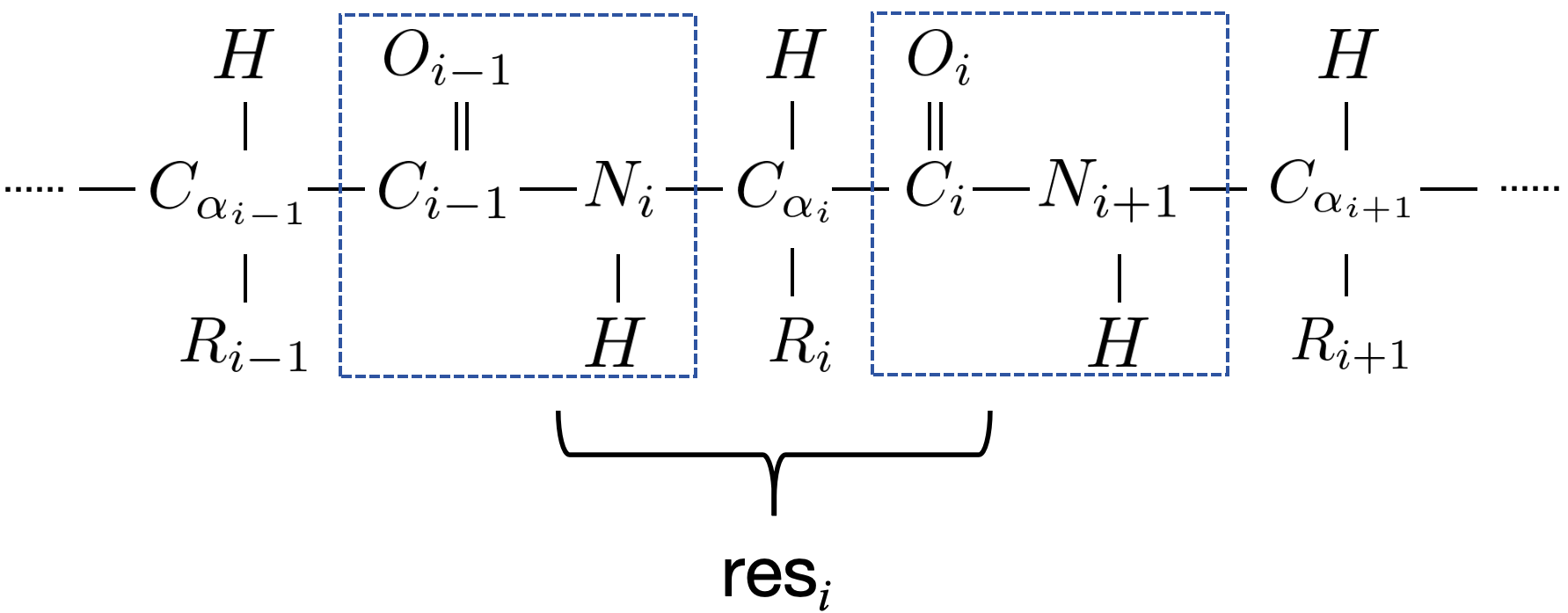
Figure 1. A peptide chain. The backbone of this peptide chain is the set $\{\dots,C_{\alpha_{i-1}},C_{i-1},O_{i-1},N_{i},C_{\alpha_{i}},C_{i},O_{i},\dots\}.$ Blue rectangles display the peptide bonds.

1.2. Geometry in Biology

The geometry plays important role in the study of the structure of proteins and even other biomolecules. Scientists found that three-dimensional atomic structures of these molecules provide rich information for understanding how these molecules carry out their biological functions. Among all these research, we found several cutting points that geometry can enter the study of the structures of proteins or biomolecules.

The geometry could serve as a way to represent a molecule as a solid figure. As we all know, a molecule is a system of moving particles (nuclei and electrons) which are held together by electrostatic and magnetic forces in nature. And it does not possess any definitive boundaries. However, visualizing a molecule is still a very useful chemical concept and has proved its value in medicinal chemistry.

The van der Waals radius of an atom, denoted as $r_{w}$, is the radius of an imaginary hard sphere representing the distance of closest approach for another atom. The van der Waals surface of a molecule is an abstract representation or model of that molecule by treating each atom as a sphere with the van der Waals radius. This model is named for Johannes Diderik van der Waals, a Dutch theoretical physicist and thermodynamicist. Several models have made improvements towards the van der Waals surfaces. The CPK models is developed by and named for Robert Corey, Linus Pauling, and Walter Koltun in the paper [16]. In this model, atoms were represented by spheres whose radii were proportional to the van der Waals radii of the atoms, and whose center-to-center distances were proportional to the distances between the atomic nuclei in the same scale. The Lee-Richards surface model, raised by B.Lee and F.M.Richards in the paper [36], was given by the center of a radius $r_{w}$ sphere when this ball was rolling everywhere along the van der Waals surface of the molecule. While Lee-Richards surface might not be smooth, the Connolly’s surface model, introduced by M.L.Connolly in [15], was constructed by replacing the center by the ‘front’ of the same sphere.

On the other hand, it was found in biology that low-energy elements occur more frequently than others in the 3D structure of proteins. This interesting phenomenon was summarized as the Boltzmann like statistics for proteins, i.e.,

(1) $$\hbox{OBSERVED OCCURRENCE}\sim exp(-\frac{\hbox{ENERGY}}{RT^{\ast}})$$

where $T^{\ast}$ is the ‘conformational temperature’ of protein statistics which is close to room temperature, and $R$ is the Boltzmann constant [24, 25]. From this point of view, geometry objects could enter as representations of biomolecules. For example, the most commonly known theory in this side is the Ramachandran plot for proteins raised in [59]. In this theory, people focused on two backbone dihedral angles $\psi$ and $\phi$ of residues in proteins. The Ramachandran plot visualized energetically allowed regions for $\psi$ against $\phi$.

The existence of hydrogen bonds, especially the backbone hydrogen bond (BHB), is also important in the formation of the structure of proteins and the realization of the functions of proteins. Following the same philosophy of Equation 1, the Backbone Free Energy Estimator was introduced by R.Penner in [56, 55]. In this theory, he constructed the unit 3D frames on both sides of BHB with $x-y$ plane is the peptide plane and $z$ axis is the associated cross product. Hence, he could represent a BHB as an element on the Lie group $\operatorname{SO}_{3}(\mathds{R})$. The distribution of BHBs on $\operatorname{SO}_{3}(\mathds{R})$ could be computed from a well-selected data set.

The energy also appears in the studies and simulations of variations of protein conformations. This is a joint field of differential geometry, the shape analysis and biology. The shape space is somehow like the moduli space in mathematics. Since the energy usually appears as a sum of the potential of interactions that only depend on the Euclidean distance between pairs of atoms in the protein. Two conformations can only be distinguished up to rigid-body transformations. This observation gives the idea of the shape space. The shape space is a quotient manifold by identifying each protein conformation with the orbit space of configuration space of all protein conformations by its rigid-body transformations. The dynamics of the protein conformation could be treated as the flow or the deformation on the shape space. There are several ways of constructing the shape spaces, for example using the backbone dihedral angles, using the point cloud and the Normal mode analysis (NMA) [6, 27, 7]. The Backbone Free Energy Estimator [56, 55] introduced above with the shape space $\operatorname{SO}_{3}(\mathds{R})$ is another example. Shape space is an important object in shape analysis and computer vision, we refer [9, 35, 75] for more detailed introduction.

Finally, let us mention a recent work [18] trying to bring the Riemannian geometry into the study of the protein conformations. In this paper, they constructed a smooth manifold from the quotient of the configuration space of non-planer atom coordinates by the group of affine translations. The different conformations of the proteins were represented as points on this manifold. An energy motivated and efficiently evaluated metric could be defined on this manifold such that making this manifold a Riemannian manifold. Then the dynamics of changing of protein conformations could be efficiently interpolated and extrapolated along non-linear geodesic curves.

1.3. Discrete Curve Model

Many topics in applied geometry like computer graphics and computer vision have close connection with discrete geometry, especially the discrete curves and discrete surfaces. For example, the tasks like analysis of geometric data, its reconstruction, and further its manipulation and simulation. Approximations of 3D-geometric notions play a crucial part in creating algorithms that can handle such tasks. Similarly as the smooth realm where the curvature and torsion play important roles in parametrizing a smooth curve or surface, the estimation of curvatures and torsions of curves and surfaces is also important in applied geometry.

Recall that the curvature of a smooth curve $\gamma$ at a fixed point $p$ is defined as the inverse of the radius of the osculating circle of $\gamma$ at point $p$. It quantifies the extent of the bending of $\gamma$ at $p$. The torsion of the curve $\gamma$ is given by the ’percentage’ between the normal bundle of the curve and the projection of the differential of the binormal bundle on the normal bundle. It measures the speed of a smooth curve moves away from it osculating plane. In the discrete case, we applied the ideas and methods from classical differential geometry instead of “simply” discretizing equations or using classical differential calculus. There are several versions of discretized curvature and torsion based on using different starting point of the classical differential geometry like from Frenet-frame [8] and from geometric knot theory [68].

In this paper, we mentioned two ways of applying properties of the discrete curve. The first, which we call it the truncated Hop distance between two discrete curves, is defined as a matrix composed of the differences of hop distances of vertices between two discrete curves. We will show below by example that treating a protein as a discrete curve and applying this simply defined and computed parameter give us an important property in the formation of amyloid fibril. We will show below by example that by treating a protein as a discrete curve, this simply defined and computed parameter give us an important property of the formation of amyloid fibril.

On the other hand, we introduced a version of discrete curvature and torsion from [48] which is based on the osculating circle of a discrete curve. We will introduce an example that this version of torsion could detect the BHB between layers of amyloid fibril.

1.4. Topological Model

Topological Data Analysis (TDA) is a mathematical field focus on the ‘shapes’ of the data. It provides a set of mathematical and computational techniques to analyze complex high-dimensional data, and identify key features of the data which may be difficult to be extracted with traditional methods. Recently, TDA has been witnessed applications in a variety of disciplines, such as computational chemistry [70], nano material [73], environmental science [52, 53], natural language processing [23], image segmentation [14], medical imaging [64, 46, 57], deep learning model [58, 12], complex network [26, 72], economy [63], biomolecular analysis [17, 39], the winning of D3R Grand Challenges [49, 50] and the evolutionary mechanism of SARS-CoV-2 [11], etc. Compared with traditional dimensionality reduction methods, such as principal component analysis (PCA), TDA retains more effective information while reducing the dimensionality of data.

Up to now, various tools have been developed under the heading of TDA, such as (i) Mapper. Mapper first divides the original data into several clusters based on the preassigned filter functions. Then, two clusters are connected if they have common data points. The output of mapper is a combinatorial graph. Monica N. et al. analyzed the microarray gene expression data by adopting Mapper and disease-specific genomic analysis transformation, and successfully identified a unique subgroup of Estrogen Receptor-positive (ER+) breast cancers[51]. (ii) Persistent topological laplacians (PDL). PDL captures information about data based on the spectra of the laplacian operator. Specifically, the harmonic spectra relates to the Betti number of data, while the non-harmonic spectra provides extra geometry information [29, 38]. PDL-based approaches have been applied to analyze the structure of protein-protein interaction networks [19]. (iii) Persistent homology (PH). PH is one of the most popularly used tool in TDA, which creates a multiscale family of simplicial complexes and describes the evolution of these complexes and their associated homology groups over scales. We will focus on the PH in the following materials.

Persistent homology has been widely applied in data science, such as crystalline material [33], chemical engineering[65], especially computational biology[39]. For example, the element-specific PH combined with deep learning winned the D3R Grand Challenges[49, 50], the element- and site-specific PH adopted for prediction the evolutionary mechanism of SARS-CoV-2[11] and hypergraph-based PH to predict protein-ligand binding affinity[40]. Theories related to PH have been developed rapidly, including weighted PH [60, 3], multiparameter PH [28, 61, 41], etc. Moreover, the open source packages, such as Gudhi [42], Javaplex [1], Ripser[2], etc., have contributed to the wide range of applications in different areas of PH. In this paper, we introduced basic definitions of the PH. More details can be found in [77, 20]. Moreover, We will give an example of the application showing that these tools give better indicators to distinguish amyloid fibrils than the commonly used indicator RMSD.

1.5. Arrangement of the Paper

The reminder of this paper is organized as follows. In Section 2, we defined the truncated Hop distance to compare the structure of two discrete curves. Moreover, we explained how to treat one layer of amyloid fibril as a discrete curve. And we suggest that the effect in the formation of amyloid fibril is relatively mild based on the result of the truncated Hop distance. Preliminaries of the definitions of curvature and torsion on the discrete curves are presented in Section 3. By computing the discrete curvature and torsion on single layers of amyloid fibril, we suggest that the anomalies reflect slight affects of the layer-layer hydrogen bonds. Finally in Section 4, we introduced the distances between persistent diagrams (PDs), and showed that how these distances work in quantifying the difference of the structure of amyloid fibrils.

2. Discrete Curve and Hop Distance

A discrete curve is a polygonal curve in $\mathds{R}^{2}$ or $\mathds{R}^{3}$ given by its vertices via a map $\gamma:\mathds{Z}\to\mathds{R}^{3}$. In this section, we will introduce a direct parameter that not only could distinguish two different discrete curves, but also showed meaning in analyzing the difference of the structure of protein with well-folded form and amyloid form.

2.1. Hop distance

Let $\gamma$ and $\gamma^{\prime}$ be two different discrete curves, and $\gamma_{i}$ and $\gamma^{\prime}_{i}$ be the corresponding points of vertices. Let $d(\gamma_{i},\gamma_{i+k})$ be the Euclidean distance between the $i$-th and $(i+k)$-th vertices, also called the $k$-hop distance between $\gamma_{i}$ and $\gamma_{i+k}$.

Definition 2.1.

The $N$-truncated hop distance, where $N$ is a fixed positive integer, between the two discrete curve $\gamma$ and $\gamma^{\prime}$ is given by the $N\times N$ matrix $D$ with

(2) $$D_{ij}=|d(\gamma_{i},\gamma_{j})-d(\gamma_{i}^{\prime},\gamma_{j}^{\prime})|.$$

2.2. Applications to Analysis of the Structure of Amyloid fibrils

To explore structural or functional properties of proteins in practice, we mostly consider the heavy atoms of residues, the backbone of peptide chain, or the set of $C_{\alpha}\text{s}$ [5, 71] to simplify the structure of protein. This simplication reduce the redundant and irrelevant information, but also preserve the significant structural features of proteins, which can improve the efficiency of research. In this case, we may treat a peptide chain as a discrete curve to explore its geometry invariants. It could be helpful to extract the structural features of protein, and further, to analyze the functions of protein. In this example, we focused on the analysis of the structure of point mutant V30M TTR with well-folded form and amyloid form, as shown in Fig.2.

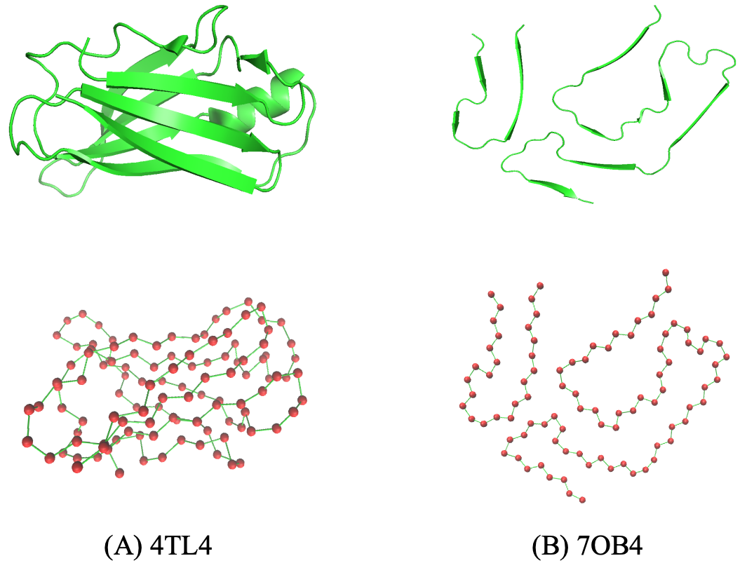
Figure 2. Convert peptide chains into discrete curves. (A) The top is the cartoon representation of chain A of TTR V30M mutant (PDB entry: 4TL4), and the bottom is its corresponding discrete curve. (B) The top is the cartoon representation of chain A of one amyloid form of 4TL4 (PDB entry: 7OB4), and the bottom is its corresponding discrete curve. Red balls represent the $C_{\alpha}$ atoms.

It has been discovered that amyloid fibril serves as the key pathological entity in different neurodegenerative diseases, such as Alzheimer’s disease and Parkinson’s disease [54, 34]. However, the process by which amyloid fibril is formed is so far obscure, hindering further research into the causes of diseases. Here, we used the truncated hop distance to explore the strength of effect in the formation of amyloid form, as shown in Fig.3.

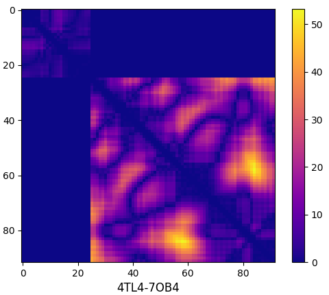
Figure 3. The truncated hop distance between chain A of 4TL4 and 7OB4. The unit is the Angstrom (Å).

It is clear that the values near the diagonal is less than 1.5Å, which illustrates that there could not be stretching and compressing in the process of the formation of amyloid fibril. We suggest that the effect is relatively mild in the formation from chain A of 4TL4 to chain A of 7OB4.

3. Discrete Curvatures and Discrete Torsions

The discrete torsion based on the cross ratio and osculating circle was first introduced in [48], which is used in computer vision to estimate the differences between the background smooth curve and the discrete sample curve. In the paper [37], we introduced this important parameter to the analyzing the structure of proteins. We found that compared with the traditional tools like backbone dihedral angles, discrete curvature resp. discrete torsion is a order two resp. order three parameter which is more sensitive to the weak interactions. In this section, we will give a detailed introduction on these parts.

3.1. Curvatures and Torsions for Smooth Curves

The curvature and the torsion are two important geometric invariants parametrizing the property of a smooth space curve. We will first recall the corresponding constructions in the smooth case. Let $\gamma(s)\subset\mathds{R}^{3}$ be a smooth space curve with $s$ the arc length parameter. Recall that the tangent field $T(s)$ is unit for all $s\in\mathds{R}$. The principal normal field is given by $N(s):=\frac{T^{\prime}(s)}{\parallel T^{\prime}(s)\parallel}$ and the binormal field by $B(s):=N(s)\times T(s)$ while both of them are unit vector fields. It is clear that the three unit vectors $T(s),\ N(s)$ and $B(s)$ are pairwise normal, hence they form a frame at each point.

The curvature $\kappa$ is defined as $\kappa:=\parallel T^{\prime}(s)\parallel$ parametrizing the bending degree of the curve. Geometrically, there exists a space circle passed $\gamma(s)$ which has $N(s)$ as radial vector and $\frac{1}{\kappa}$ as radius. This circle is called the osculating circle, which has contact of order at least 2 with $\gamma$ at $\gamma(s)$. Therefore, they have the common tangent plane which is spanned by $T(s)$ and $N(s)$ and we call it the osculating plane.

Since $B(s)$ is an unit field, its differential $B^{\prime}(s)$ should tangent to $B(s)$. Moreover, it is clear that the following equation holds.

(3) $$0=\frac{d}{ds}<B(s),T(s)>=<B^{\prime}(s),T(s)>+<B(s),T^{\prime}(s)>=<B^{\prime}(s),T(s)>$$

Hence, $B^{\prime}(s)$ should parallel to $N(s)$, the torsion of the curve $\gamma$ at $\gamma(s)$ as the number $\tau$ satisfying the property that $B^{\prime}(s)=-\tau N(s)$. From all these constructions, the torsion $\tau$ parametrized the speed of a curve moving away from its osculating plane.

3.2. Basics in quaternions

Let $\mathds{H}$ be the ring of quaternionics which could be treated as a skew field whose elements can be identified with $\mathds{R}\times\mathds{R}^{3}$. There exist an isomorphism of Euclidean 3-space $\mathds{R}^{3}$ with the imaginary parts of $\mathds{H}$. In this paper, we will write $\mathds{H}$ in the following way

(4) $$\mathds{H}:=\{[r,v]:r\in\mathds{R},v\in\mathds{R}^{3}\}$$

The first part $r=\operatorname{Re}q$ resp. the second part $v=\operatorname{Im}q$ of a quaternion $q=[r,v]$ is called the real part of $q$ resp. the imaginary part of $q$. The set of all pure imaginary quaternions is denoted as $\operatorname{Im}\mathds{H}$, i.e., $\operatorname{Im}\mathds{H}:=\{[0,v]:v\in\mathds{R}^{3}\}$. Some operators on $\mathds{H}$ under this form are listed in the Table 1.

Addition	$[r,v]+[s,w]=[r+s,v+w]$
Multiplication	$[r,v]\cdot[s,w]=[rs-<v,w>,rw+sv+v\times w]$
Conjugation	$\overline{q}=[r,-v]$
Norm	$|q|=\sqrt{q\cdot\bar{q}}=\sqrt{r^{2}+\parallel v\parallel^{2}}$
Inverse	$q^{-1}=\frac{\bar{q}}{|q|}$
Cross Ratio	$\operatorname{cr}(a,b,c,d):=(a-b)(b-c)^{-1}(c-d)(d-a)^{-1}$

Table 1. Some operators on $\mathds{H}$

In this paper, the polar representation of a quaternion is quite useful, for a quaternion $q=[r,v]$ its polar representation is defined as $q=|q|[\cos\phi,v\sin\phi]$ with $\parallel v\parallel=1$ and $\phi\in[0,\pi]$. In this case, the square root of $q$ is defined as $\sqrt{q}:=\sqrt{|q|}[\cos\frac{\phi}{2},v\sin\frac{\phi}{2}]$. Note that such defined square root is not unique if $q\in\mathds{R}_{\leq 0}$, however, we will not meet this case in our application.

Recall that a Möbius transformation is a homeomorphism of $\mathds{R}^{n}\cup\{\infty\}$ which is a finite composition of inversions in spheres and reflections in hyperplanes. In other words, any Möbius transformation $\sigma$ can be written as the form

(5) $$\sigma(x)=x+\frac{\alpha A(x-a)}{\parallel x-a\parallel^{\epsilon}},\ x\in\mathds{R}^{n}\cup\{\infty\}$$

where $\alpha\in\mathds{R}$, $a,b\in\mathds{R}^{n}$, $A$ is an orthogonal matrix and $\epsilon$ equals 0 or 2. It is clear to check that the cross-ratio above is invariant under Möbius transformation i.e. the following equation holds for all Möbius transformation $\sigma$

(6) $$\operatorname{cr}(\sigma(a),\sigma(b),\sigma(c),\sigma(d))=\operatorname{cr}(a,b,c,d)$$

Moreover, we have the following Lemma for the properties of the cross ratio.

Lemma 3.1.

Let $a,b,c,d,d^{\prime}\in\mathds{H}$ be four quaternions, then we have

1. If $d^{\prime}\in\mathds{H}$, $a\neq c$ and $\operatorname{cr}(a,b,c,d)=\operatorname{cr}(a,b,c,d^{\prime})$, then we have $d=d^{\prime}$.

2. If $a,b,c,d\in\operatorname{Im}\mathds{H}\cong\mathds{R}^{3}$, then $\operatorname{cr}(a,b,c,d)\in\operatorname{Re}\mathds{H}$ if and only if $a,b,c,d$ are concyclic.

Proof.

1. The first is clear to check.

2. The second is proved in [4].

∎

Lemma 3.2.

Let $a,b,c,d\in\operatorname{Im}\mathds{H}$ be four points not lying on a common circle. Then, the imaginary part of the cross-ratio is the normal of the circumsphere (or plane) at $a$, i.e., for a proper circumsphere with center $m$, we have $\operatorname{Im}\operatorname{cr}(a,b,c,d)\mathrel{/\mskip-2.5mu/}(m-a)$.

Remark 3.3.

If the four points $a,b,c,d$ are coplaner, then $m$ is the point of $\infty$. The vector $\operatorname{Im}\operatorname{cr}(a,b,c,d)$ is orthogonal to the common plane of $a,b,c,d$.

Proof.

This is Lemma 10 of [48]. ∎

Let us define the ‘diagonal’ points $f(a,b,c,d)$ as

(7) $$f(a,b,c,d):=((b-a)(c-a)^{-1}\sqrt{\operatorname{cr}(c,a,b,d)}+1)^{-1}((b-a)(c-a)^{-1}\sqrt{\operatorname{cr}(c,a,b,d)}c+b)$$

We have the following lemmas

Lemma 3.4.

The ‘diagonal’ point $f(a,b,c,d)$ fullfills the equation that

(8) $$\operatorname{cr}(c,a,b,f(a,b,c,d))=-\sqrt{\operatorname{cr}(c,a,b,d)}$$

Moreover if we assume $a,b,c,d\in\operatorname{Im}(\mathds{H})\cong\mathds{R}^{3}$ then the ’diagonal’ point satisfies $f(a,b,c,d)\in\operatorname{Im}(\mathds{H})$. Even more $f(a,b,c,d)$ lies on the circumsphere of $a,b,c,d$.

Remark 3.5.

If $a,b,c,d$ are four points in $\mathds{R}^{3}\cong\operatorname{Im}\mathds{H}$ that form a parallelogram with $ab$ parallel to $cd$, the inserting point $f(a,b,c,d)$ is the intersection of the two diagonals $ac$ and $bd$. This is the reason that it is called a ‘diagonal’ point.

Corollary 3.6.

The formula $f$ is invariant under Möbius transformation.

Proof.

The Lemma 3.4 is the Lemma 11 and Corollary 4 in [48]. Then from the Lemma 3.1 and Lemma 3.4 the formula $f$ is Möbius transformation invariant. ∎

Now we will introduce one of the most important Proposition and also the basis of the further construction.

Proposition 3.7.

Let $a,b,c,d\in\operatorname{Im}\mathds{H}\cong\mathds{R}^{3}$ be four pairwise different points and consider the four inserting points given by $f$ and cyclic permutations

(9) $$A=f(d,a,b,c) B=f(a,b,c,d)$$

(10) $$C=f(b,c,d,a) D=f(c,d,a,b)$$

Then the four points $A,B,C,D$ are concyclic with

(11) $$\operatorname{cr}(A,B,C,D)=-1$$

Proof.

We only need to prove the Equation 11 holds. From Lemma 3.4 the four points $A,B,C$ and $D$ lie on a common sphere i.e. the circumsphere of $a,b,c,d$. Let us fix an unit vector $v_{0}\in\mathds{R}^{3}$. It is clear that the space $\mathds{C}_{v_{0}}:=\{[r,kv_{0}]:r,v\in\mathds{R}\}$ is isomorphic to the complex plane $\mathds{C}$. Let $\sigma$ is the Möbius transformation that maps the circumsphere of $a,b,c,d$ to $\mathds{C}_{v_{0}}$.

From Lemma 3.1, that we have $\operatorname{cr}(A,B,C,D)=\operatorname{cr}(\sigma(A),\sigma(B),\sigma(C),\sigma(D))$. Hence without loss of generality, we may assume $a,b,c,d$ are both complex numbers. In this case, the Equation 11 comes from a direct compute, the details are in Theorem 1 of [48]. ∎

3.3. Curvatures and Torsions for Discrete Curves

Let us consider the discrete case. Recall that a discrete curveis a polygonal curve in $\mathds{R}^{2}$ or $\mathds{R}^{3}$ given by its vertices via a map $\gamma:\mathds{Z}\to\mathds{R}^{3}$. We will see the definition of curvature and torsion for a discrete curve follows similar philosophy as their smooth versions. Historically, the curvature for a discrete curve has a long history and is widely used in computer vision and study of complex networks. However, the torsion is pretty new, one is first introduced in [48]. We will introduce them in this section.

Let $\gamma_{i}$ be a vertex of the discrete curve. From the Proposition 3.7, for each four elements tuple $(\gamma_{i-1},\gamma_{i},\gamma_{i+1},\gamma_{i+2})$ there exist four inserting points i.e.

(12) $$A_{i} = f(\gamma_{i+2},\gamma_{i-1},\gamma_{i},\gamma_{i+1}),\ B_{i} = f(\gamma_{i-1},\gamma_{i},\gamma_{i+1},\gamma_{i+2})$$

$$C_{i} = f(\gamma_{i},\gamma_{i+1},\gamma_{i+2},\gamma_{i-1}),\ D_{i} = f(\gamma_{i+1},\gamma_{i+2},\gamma_{i-1},\gamma_{i})$$

The Lemma 3.4 implies that the four points lie on the circumsphere of $\gamma_{i-1},\gamma_{i},\gamma_{i+1}$ and $\gamma_{i+2}$ which we take it as the discrete osculating sphere at $\gamma_{i}$. Note that $\gamma_{i-1},\gamma_{i},\gamma_{i+1}$ and $\gamma_{i+2}$ are not concyclic in general, but the Proposition 3.7 implies that the four points $A_{i}$, $B_{i}$, $C_{i}$ and $D_{i}$ are concyclic.

Definition 3.8.

Let $\gamma$, $\gamma_{i}$,$A_{i}$,$B_{i}$,$C_{i}$ and $D_{i}$ as above, the circle denoted by $k_{i}$ given by $A_{i}$,$B_{i}$,$C_{i}$ and $D_{i}$ is the osculating circle of $\gamma$ at $\gamma_{i}$. The inverse of the radius of $k_{i}$ the discrete curvature at $\gamma_{i}$ denoted by $\kappa_{i}$.

Definition 3.9.

The normal unit vector $N_{i}$ of $\gamma$ at $\gamma_{i}$ to be the unit normal vector of $k_{i}$ at $B_{i}$. The plane passing through $B_{i}$ and normal to $N_{i}$ as the osculating plane.

Definition 3.10.

The discrete torsion of $\gamma$ at $\gamma_{i}$ is defined as following

(13) $$\tau_{i}:=-\frac{9<\operatorname{Im}\operatorname{cr}(\gamma_{i-1},\gamma_{i},\gamma_{i+1},\gamma_{i+2}),N_{i}>}{2\kappa_{i}\parallel\gamma_{i}-\gamma_{i+1}\parallel^{2}}$$

Remark 3.11.

The connection of discrete torsion and smooth version are as following: Let us assume in this Remark that $\gamma(t)$ be a smooth curve and $t$ be any parameter. In this case the torsion of $\gamma$ at $\gamma(t_{0})$ could be computed as

(14) $$\tau = -\frac{<\gamma^{\prime}\times\gamma^{\prime\prime},\gamma^{\prime\prime\prime}>}{\parallel\gamma^{\prime}\times\gamma^{\prime\prime}\parallel^{2}} = -\frac{\det(\gamma^{\prime},\gamma^{\prime\prime},\gamma^{\prime\prime\prime})}{\parallel\gamma^{\prime}\times\gamma^{\prime\prime}\parallel^{2}}$$

$$= \frac{\det(\gamma^{\prime\prime\prime},\gamma^{\prime},\gamma^{\prime\prime})}{\parallel\gamma^{\prime}\times\gamma^{\prime\prime}\parallel^{2}} = \frac{<\gamma^{\prime}\times\gamma^{\prime\prime\prime},\gamma^{\prime\prime}>}{\parallel\gamma^{\prime}\times\gamma^{\prime\prime}\parallel^{2}}$$

Recall that $\kappa=\frac{\parallel\gamma^{\prime}\times\gamma^{\prime\prime}\parallel}{\parallel\gamma^{\prime}\parallel^{3}}$ and

(15) $$N=B\times T=\frac{\gamma^{\prime\prime}<\gamma^{\prime},\gamma^{\prime}>-\gamma^{\prime}<\gamma^{\prime},\gamma^{\prime\prime}>}{\parallel\gamma^{\prime}\times\gamma^{\prime\prime}\parallel\parallel\gamma^{\prime}\parallel}=\frac{1}{\parallel\gamma^{\prime}\parallel^{2}\kappa}\gamma^{\prime\prime}-\frac{<\gamma^{\prime},\gamma^{\prime\prime}>}{\parallel\gamma^{\prime}\times\gamma^{\prime\prime}\parallel\parallel\gamma^{\prime}\parallel}\gamma^{\prime}$$

Hence, we have the following

(16) $$\tau=\frac{<\gamma^{\prime}\times\gamma^{\prime\prime\prime},N>}{\kappa\parallel\gamma^{\prime}\parallel^{4}}$$

In the discrete case, the role of $\gamma^{\prime}\times\gamma^{\prime\prime\prime}$ is replaced by $\operatorname{Im}\operatorname{cr}(\gamma_{i-1},\gamma_{i},\gamma_{i+1},\gamma_{i+2})$. We will show below that such defined discrete torsion satisfies our expectations.

Now let us introduce without proof several properties of the definitions above which reveal the fact that the discrete curvature, normal vector and torsion defined above is the approximation of the smooth version.

Proposition 3.12.

The discrete torsion vanishes for planer discrete curve.

Proof.

If $\gamma$ is a discrete curve lying on the plane $P$, the vector $\operatorname{Im}\operatorname{cr}(\gamma_{i-1},\gamma_{i},\gamma_{i+1},\gamma_{i+2})$ is orthogonal to $P$ from the Lemma 3.2. From the Definition 3.9, $N_{i}\subset P$. Hence the discrete torsion vanish at all points. ∎

Theorem 3.13.

Let $s:\mathds{R}\to\mathds{R}^{3}$ be a smooth space curve, let $\mu,\epsilon\in\mathds{R}$ be real numbers and let the discrete curve $\gamma:\mathds{Z}\to\mathds{R}^{3}$ with $\gamma_{i}:=s(\mu+(2i-1)\epsilon)$ be the sample of $s$. Let $\kappa$, resp. $N$ and $\tau$ be the curvature reps. unit normal vector and torsion of $s$ at $s(\mu)$. We have the following properties

1. The discrete curvature is a second approximation of $\kappa_{s}$, i.e. $\kappa_{0}=\kappa_{s}+o(\epsilon^{2})$,

2. The center $m_{0}$ of the discrete osculating circle $k_{0}$ of $\gamma$ converges to the center of the smooth osculating circle of $s$ at the same rate, i.e. $m_{0}-s(\mu)=\frac{N(\mu)}{\kappa_{s}(u)}+o(\epsilon^{2})$,

3. The discrete Frenet frame $(T_{0},N_{0},B_{0})$ is a second-order approximation of the smooth Frenet frame $(T,N,B)$,

4. The discrete torsion is a second-order approximation of the smooth torsion i.e. $\tau_{0}=\tau+o(\epsilon^{2})$

Proof.

This is the Theorem 4, Lemma 14, Lemma 15 and Theorem 5 in [48]. The main points is similar as the proof of the Proposition 3.7, we first map all points to a complex plane by a Möbius transformation. Then we could check by direct computation. ∎

3.4. Applications to Analysis of the Structure of Amyloid fibrils

We have shown a way of treating a peptide chain as a discrete curve and its application in the Section 2. In this section, we considered another way as following: Recall that from the Figure 1, the backbone consists of amino nitrogens, $\alpha$-carbons, carbonyl carbons and carbonyl oxygens. For a fixed peptide chain which is also a layer of the amyloid fibrils, let $N_{i}$ resp. $C_{\alpha_{i}}$ and $C_{i}$ be the coordinates of amino nitrogens resp. $\alpha$-carbons and carbonyl carbons with $i\in\mathds{Z}^{\geq 1}$ being the indices of the residues in this layer. This is a discrete curve whose vertices points are $N_{i}$, $C_{\alpha_{i}}$ and $C_{i}$. By applying the definitions in Section 3, we will compute the curvatures and torsions as below

(17) $$C_{i-1},N_{i},C_{\alpha_{i}},C_{i} \to \hbox{Curvatures and Torsions at }N_{i}$$

$$N_{i},C_{\alpha_{i}},C_{i},N_{i+1} \to \hbox{Curvatures and Torsions at }C_{\alpha_{i}}$$

$$C_{\alpha_{i}},C_{i},N_{i+1},C_{i+1} \to \hbox{Curvatures and Torsions at }C_{i}$$

The pseudo-code of computing curvature and torsion is shown as the Algorithm 1.

1

input : A series of shape $3l\times 3$ consists of coordinates of all amino nitrogens, $\alpha$-carbons and carbonyl carbons

output : A series of shape $3l\times 2$ consists of curvatures and torsions at each atom

2 for $i\leftarrow 1$ to $l-3$ do

3      

4      compute inserting points $A,B,C,D$

5      compute circumcircle center $O$ by solving equations

$$(X-\frac{A+B}{2})\overrightarrow{BA} = 0$$

$$(X-\frac{A+C}{2})\overrightarrow{CA} = 0$$

$$(\overrightarrow{AB}\times\overrightarrow{AC})\overrightarrow{XA} = 0$$

6      compute $\kappa=\frac{1}{\parallel\overrightarrow{AO}\parallel}$

7      compute $N=\frac{\overrightarrow{AO}}{\parallel\overrightarrow{AO}\parallel}$

8      compute torsion $\tau$

9 end for

Algorithm 1 Algorithm of computing curvature and torsion

We conducted the computation to several amyloid fibrils. We found that the torsions at carbonyl carbons are significantly larger than the one in other places (we list one example 7OB4 in Figure 4). We showed that this anomalies reflect slight affects of the layer-layer hydrogen bonds. Without loss of generality, we may assume the nearby three layers of 7OB4 is marked as A,B and C. We processed the correlation analysis between $|\tau_{i}|$, the absolute value of torsion, and $|(\tilde{d}^{i}_{B,-})^{2}-(\tilde{d}^{i}_{B,+})^{2}|$, where $\tilde{d}^{i,-}_{B}$ is the Euclidean distance of $O_{i}(B)$ and $N_{i+1}(A)$ and $\tilde{d}^{i,+}_{B}$ is the Euclidean distance between $O_{i}(B)$ and $N_{i+1}(C)$. We found that although the six atoms form a peptide bond are coplaner, they have a tend to leave this plane under the influence of the layer-to-layer hydro-bond.

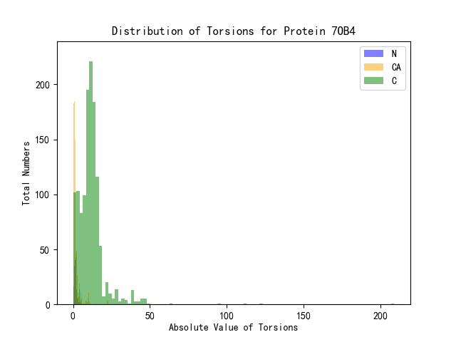
Figure 4. Distributions of absolute values of Torsions for 7OB4. The $x$-axis represents the absolute value of torsion and the $y$-axis represents the number of atoms. We take purple bar for nitrogens, orange for alpha carbons and green for carbonyl carbons. The discrete torsion is dimensionless.

Table 2. The correlation of $|\tau_{i}|$ and $|(\tilde{d}^{i}_{\cdot,-})^{2}-(\tilde{d}^{i}_{\cdot,+})^{2}|$ for 7OB4. S.D stands for the standard error

	Slope	Intercept	Pearson	$p$-value	S.D slope	S.D intercept
7OB4	-0.187	17.765	-0.194	$2.325\times 10^{-9}$	0.032	1.094

4. Topological Data Analysis

4.1. Persistent Homology in a Nutshell

We are going to introduce the definition of PH first in a general setting. Let us take $\mathds{K}$ be a fixed ring. Let $X$ be a set and $K$ be a simplicial complex constructed from $X$ which is a collection of non-empty finite subsets of $X$, such that for every set $\sigma$ in $K$ and every subset $\sigma^{\prime}\subset\sigma$, the set $\sigma^{\prime}$ also belongs to $K$. We will call $\sigma\in K$ a simplex.

Suppose further that each simplex $\sigma$ is oriented, there exists a chain complex

(18) $$\cdots\to C_{n+1}(K)\xrightarrow{\partial_{n+1}}C_{n}(K)\to\cdots$$

where $C_{n}(K)$ is the $\mathds{K}$-linear combination of simplices $\sigma=[x_{0},\cdots,x_{n}]$ in $K$ of length $n+1$ and the boundary map $\partial_{n+1}:C_{n+1}(K)\to C_{n}(K)$ is a $\mathds{K}$-linear map defined in a natural way.

Definition 4.1.

The filtration of $K$ is a nested sequence of subcomplexes $\{K_{t}\}_{t\in T}$ of $K$ with $T\subset\mathds{R}$ such that if $t\leq t^{\prime}$ then $K_{t}\subset K_{t^{\prime}}$ and $\cup_{t\in T}K_{t}=K$. Note that the index set $T$ could be finite or infinite.

Suppose $t\leq t^{\prime}$ be two different real numbers, the inclusion map $K_{t}\hookrightarrow K_{t^{\prime}}$ is also a map of chain complexes namely the following diagram commutes

(19)

where $\partial_{n}^{t}$ is the restriction of $\partial_{n}$ to $C_{n}(K_{t})$. Hence, it induces a map of homology group $H_{n}(K_{t})\to H_{n}(K_{t^{\prime}})$.

Definition 4.2.

The $(t,t^{\prime})$-persistent $n$-th homology group is defined as the image of the induced map $H_{n}(K_{t})\to H_{n}(K_{t^{\prime}})$. In other words, it is the following group

(20) $$H_{n}^{t\to t^{\prime}}=Z_{n}^{t}/(B_{n}^{t^{\prime}}\cap Z_{n}^{t}),$$

where $Z_{n}^{t}$ is the $n$-th cycle group of $K_{t}$, i.e., $\ker\partial_{n}^{t}$, and $B_{n}^{t^{\prime}}$ is the $n$-th boundary group of $K_{t^{\prime}}$, i.e., $\operatorname{Im}\partial_{n+1}^{t^{\prime}}$. The rank of $H_{n}^{t\to t^{\prime}}$ is called the $(t,t^{\prime})$-persistent $n$-th Betti number denoted as $\beta_{n}^{t\to t^{\prime}}$.

The value $t_{0}$ where for every $\delta>0$ the induced map $H_{n}(K_{t_{0}-\delta})\to H_{n}(K_{t_{0}+\delta})$ is not an isomorphism is called a homological critical value.

Remark 4.3.

In the real world applications, people always assume the coefficient ring $\mathds{K}$ to be $\mathds{Z}/2\mathds{Z}$ in which case the orientation of the simplex is not important, since in such circumstances the boundary of the simplex is not related to the orientation. Hence we will usually omit the choice of orientation in the TDA process.

Definition 4.4.

A persistence $\mathds{K}$ module $M$ is a family of $\mathds{K}$-modules $M_{i}$, together with homomorphisms $\varphi_{i}:M_{i}\to M_{i+1}$. We say a persistence module $M$ of finite type if each component module is a finitely generated $\mathds{K}$-module, and if there exist positive integer $m_{0}$ such that the maps $\varphi$ are isomorphisms for $i\geq m_{0}$.

Remark 4.5.

There exists a functor from the category of persistence modules of finite type over $\mathds{K}$ to the category of finitely generated non-negatively graded modules over the polynomial ring $\mathds{K}[x]$, namely take the grade on $M$ as the natural one and $x$ acts on $M$ via the map $x\to\varphi$. From the Artin-Rees theory [22], this construction turns out to be an equivalence of categories.

From our requirements, from now on let us assume in additional that $\mathds{K}$ is a field and the above simplicial complex $K$ is finite. This means each group in chain complex 18 is a finite dimensional vector space over $\mathds{K}$. In this case, the ‘filtration’ on the chain complex 18, which will be called a persistent complex[77], is actually of finite length. In other words, the total chain complex $C(K)$ and the homology module $H(C(K),\mathds{K})$ are both persistent module of finite type. The total chain complex $C(K)$ is not only a graded $\mathds{K}$-module but also a $\mathds{K}[x]$-module with the variable $x$ of degree 1 acts as shift map via the filtration. The total homology module $H(C(K),\mathds{K})$ retains this $\mathds{K}[x]$-module structure. And from the structure theorem for principal integral domains (PID), note that $\mathds{K}[x]$ is a PID for a field $\mathds{K}$, we have the following decomposition

(21) $$H(C(K),\mathds{K})\cong\mathop{\oplus}\limits_{i}x^{t_{i}}(\mathds{K}[x])\oplus(\mathop{\oplus}\limits_{j}x^{r_{j}}(\mathds{K}[x]/(x^{s_{j}}\mathds{K}[x])))$$

Here $t_{i}$, $r_{j}$ and $s_{j}$ are all integers represent index of filtration. The decomposition theorem has the following meaning: the free parts of Equation 21 are in bijective correspondence with those homology generators birth at parameter $t_{i}$ and persist for all future parameter values. The torsion parts correspond to those homology generators birth at parameter $r_{j}$ and death at parameter $r_{j}+s_{j}$.

PD is one of the common visualization methods of the PH. PD is a multiset of points in the extended two-dimensional plane $\overline{\mathds{R}}^{2}$ where $\overline{\mathds{R}}=\mathds{R}\cup\infty$, whose coordinates are respectively correspond to the birth and death time of the homology generators, union the diagonal points [20]. Given two PDs $P_{1}$ and $P_{2}$, there are two commonly used metrics to compare them, that is, the Wasserstein-$q$ distance $W_{q}$ and Bottleneck distance $W_{\infty}$. They are defined as following:

(22) $$W_{q}(P_{1},P_{2})=(\inf\limits_{\eta:P_{1}\rightarrow P_{2}}\sum\limits_{p\in P_{1}}||p-\eta(p)||_{\infty}^{q})^{\frac{1}{q}},$$

(23) $$W_{\infty}(P_{1},P_{2})=\inf\limits_{\eta:P_{1}\rightarrow P_{2}}\sup\limits_{p\in P_{1}}||p-\eta(p)||_{\infty},$$

where $\eta$ runs over all the bijections between the points in the two diagrams. The Wasserstein-$q$ distance is capable of capturing local differences in the PDs, while the Bottleneck distance is more concerned with relatively global differences.

4.2. The Vietoris-Rips (VR) complex

For different types of data, there are various complexes to characterize the data, such as (1) for point cloud data (PCD), Alpha complex, VR complex, Čech complex and Witness complex are commonly used; (2) for imaging data, cubical complex may be a good choice; (3) for graph or complex network data, path complex may perform better. By treating a layer of amyloid fibril as a discrete curve, there are several candidate complexes to characterize this PCD. Here, we adopted the VR complex since it is precise and easy to compute.

Let $X$ be a finite point set with a index in $n$-dimensional Euclidean space $(\mathds{R}^{n},d)$, where $d$ is the natural metric on the Euclidean space and $\mathds{K}$ be the field $\mathds{Z}/2\mathds{Z}$.

Definition 4.6.

The Vietoris-Rips (VR) complex (denoted by $\operatorname{VR}(X)$) of $X$ with parameter $\epsilon$ is the set of all simplices $\sigma=\{x_{0},\cdots,x_{k}\}$, such that $d(x_{i},x_{j})\leq 2\epsilon$ for all $(i,j)$.

As we explained before, the orientation of the simplex could be omitted. And there exist a natural filtration on the Vietoris-Rips (VR) complex given by the parameter $\epsilon$. Since the number of $X$ is finite, this filtration is always of finite length, i.e.,

(24) $$\emptyset=\operatorname{VR}(X)_{0}\subseteq{\operatorname{VR}(X)_{1}}\subseteq{\cdots}\subseteq{\operatorname{VR}(X)_{m}}$$

We will modify our notations a bit as follows, let $i$ and $p$ be integers

(25) $$H_{n}^{i,p}:=H_{n}^{i\to i+p}=Z_{n}^{i}/(B_{n}^{i+p}\cap Z_{n}^{i}),$$

And we have similar modification for the notations of Betti number $\beta_{k}^{i,p}:=\beta_{k}^{i\to i+p}$.

Figure 5 is the PD of the C-terminal fragment of chain A of 7OB4 using the VR complex. The data set is given by taking the coordinates of $C_{\alpha}\text{s}$ on the C-terminal fragment. Since each chain of 7OB4 is almost planner, we only computed the persistence on $H_{0}$ and $H_{1}$. Red points and blue points represent the 0-dimensional and 1-dimensional homological generators respectively in the Fig.5.

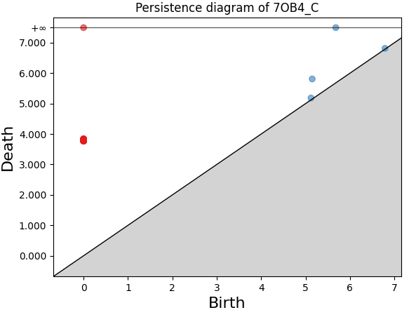
Figure 5. The PD of the C-terminal fragment of 7OB4. Red points and blue points represent the 0-dimensional and 1-dimensional homological generators, respectively. The unit is the Angstrom (Å).

4.3. Applications to Analysis of the Structure of Amyloid fibrils

The pathological function of amyloid fibril is largely determined by its structure. It is important to discriminate the structure of amyloid fibrils, followed by exploring the functions which are closely related to those structures. In biology, the RMSD is a common indicator to quantify the difference between structures after aligning. Let $\text{Prot}_{\text{1}}=\{c_{1},\dots,c_{n}\}$ and $\text{Prot}_{\text{2}}=\{c_{1}^{\prime},\dots,c_{n}^{\prime}\}$ be the coordinates of $C_{\alpha}\text{s}$ of two proteins, respectively. The RMSD between $\text{Prot}_{\text{1}}$ and $\text{Prot}_{\text{2}}$ is defined as

(26) $$\text{RMSD}=\sqrt{\frac{\sum\limits_{i=1}^{n}(c_{i}-c_{i}^{\prime})^{2}}{n}}.$$

It is clear that the RMSD only considers the difference of pairwise distance. Here, we adopted the PH to quantify the difference between two amyloid fibril structures from multiscales. The pseudo-code of comparing two amyloid fibrils is shown as the Algorithm 2. The results are listed in Table3.

Amyloid fibrils	RMSD (Å)	$W_{\infty}$(Å)	$W_{2}$(Å)	$W_{1}$(Å)
6SDZ-8ADE (N)	0.393	0.053	0.206	0.991
6SDZ-8ADE (C)	0.449	1.028	1.142	4.428

Table 3. Indicators to quantify the difference of the structure of two layers of amyloid fibrils (PDB entries: 6SDZ and 8ADE). The letter in parentheses represents the terminal fragment of chain A of each amyloid fibril.

We found that the RMSDs of two fragments are both less than 1Å. It indicates that the structure of 6SDZ and 8ADE are considered as almost the same in the RMSD context. However, the patient carries 6SDZ and the patient carries 8ADE have different clinical manifestations [66], which implies that there should be differences between the structure of these amyloid fibrils. We find that the global difference between these amyloid fibrils can be captured by the $W_{\infty}$ distance, while the local difference between these amyloid fibrils is scaled up as the exponent order $q$ decreases. PH considers the higher-order relations among these $C_{\alpha}\text{s}$, which could give us more information to distinguish the structure of amyloid fibrils.

1

input : The coordinates of atoms of two fibril structures $\text{Prot}_{\text{1}}$ and $\text{Prot}_{\text{2}}$ , the maximal filtration value $l$, the exponent order $q$

output : Distances $\{d_{\infty},d_{q}\}$ to quantify the difference between the two fibril structures

2 for $i\leftarrow 1$ to $2$ do

3       $f_{i}\leftarrow$ the filtration of $P_{i}$ based on a suitable rule, that is, $f_{i}=\{v_{j}\}_{j=1}^{n}$ where $v_{n}\leq l$

4      $\{K^{i}_{j}\}_{j=1}^{n}\leftarrow$ a nested sequence of simplicial complexes based on $f_{i}$

5      $\text{PD}_{i}\leftarrow$ the persistent homology analysis of $\{K^{i}_{j}\}_{j=1}^{n}$

6 end for

7

8$d_{\infty}\leftarrow W_{\infty}(\text{PD}_{1},\text{PD}_{2})$

$d_{q}\leftarrow W_{q}(\text{PD}_{1},\text{PD}_{2})$

Algorithm 2 Algorithm of using TDA to compare fibril structures

References

- [1] Henry Adams, Andrew Tausz, and Mikael Vejdemo-Johansson. Javaplex: A research software package for persistent (co) homology. In Mathematical Software–ICMS 2014: 4th International Congress, Seoul, South Korea, August 5-9, 2014. Proceedings 4, pages 129–136. Springer, 2014.
- [2] Ulrich Bauer. Ripser: efficient computation of vietoris–rips persistence barcodes. Journal of Applied and Computational Topology, 5(3):391–423, 2021.
- [3] Gregory Bell, Austin Lawson, Joshua Martin, James Rudzinski, and Clifford Smyth. Weighted persistent homology. Involve, a Journal of Mathematics, 12(5):823–837, 2019.
- [4] Alexander Bobenko and Ulrich Pinkall. Discrete isothermic surfaces. Journal für die reine und angewandte Mathematik, 1996.
- [5] David Bramer and Guo-Wei Wei. Atom-specific persistent homology and its application to protein flexibility analysis. Computational and mathematical biophysics, 8(1):1–35, 2020.
- [6] Bernard Brooks and Martin Karplus. Harmonic dynamics of proteins: normal modes and fluctuations in bovine pancreatic trypsin inhibitor. Proceedings of the National Academy of Sciences, 80(21):6571–6575, 1983.
- [7] Bernard Brooks and Martin Karplus. Normal modes for specific motions of macromolecules: application to the hinge-bending mode of lysozyme. Proceedings of the National Academy of Sciences, 82(15):4995–4999, 1985.
- [8] Daniel Carroll, Eleanor Hankins, Emek Kose, and Ivan Sterling. A survey of the differential geometry of discrete curves. The Mathematical Intelligencer, 36:28–35, 2014.
- [9] Nicolas Charon and Laurent Younes. Shape spaces: From geometry to biological plausibility. Handbook of Mathematical Models and Algorithms in Computer Vision and Imaging: Mathematical Imaging and Vision, pages 1–30, 2022.
- [10] Guo-fang Chen, Ting-hai Xu, Yan Yan, Yu-ren Zhou, Yi Jiang, Karsten Melcher, and H Eric Xu. Amyloid beta: structure, biology and structure-based therapeutic development. Acta Pharmacologica Sinica, 38(9):1205–1235, 2017.
- [11] Jiahui Chen, Rui Wang, Menglun Wang, and Guo-Wei Wei. Mutations strengthened sars-cov-2 infectivity. Journal of molecular biology, 432(19):5212–5226, 2020.
- [12] Yuzhou Chen, Yulia R Gel, and H Vincent Poor. Bscnets: Block simplicial complex neural networks. Proceedings of the aaai conference on artificial intelligence, 36(6):6333–6341, 2022.
- [13] Fabrizio Chiti and Christopher M Dobson. Protein misfolding, amyloid formation, and human disease: a summary of progress over the last decade. Annual review of biochemistry, 86:27–68, 2017.
- [14] James R Clough, Nicholas Byrne, Ilkay Oksuz, Veronika A Zimmer, Julia A Schnabel, and Andrew P King. A topological loss function for deep-learning based image segmentation using persistent homology. IEEE transactions on pattern analysis and machine intelligence, 44(12):8766–8778, 2020.
- [15] Michael L Connolly. Analytical molecular surface calculation. Journal of applied crystallography, 16(5):548–558, 1983.
- [16] Robert B Corey and Linus Pauling. Molecular models of amino acids, peptides, and proteins. Review of Scientific Instruments, 24(8):621–627, 1953.
- [17] Tamal K Dey and Sayan Mandal. Protein classification with improved topological data analysis. In 18th International Workshop on Algorithms in Bioinformatics (WABI 2018). Schloss-Dagstuhl-Leibniz Zentrum für Informatik, 2018.
- [18] Willem Diepeveen, Carlos Esteve-Yagüe, Jan Lellmann, Ozan Öktem, and Carola-Bibiane Schönlieb. Riemannian geometry for efficient analysis of protein dynamics data. arXiv preprint arXiv:2308.07818, 2023.
- [19] Hongyan Du, Guo-Wei Wei, and Tingjun Hou. Multiscale topology in interactomic network: from transcriptome to antiaddiction drug repurposing. Briefings in Bioinformatics, 25(2):bbae054, 2024.
- [20] Herbert Edelsbrunner, John Harer, et al. Persistent homology-a survey. Contemporary mathematics, 453(26):257–282, 2008.
- [21] David Eisenberg and Mathias Jucker. The amyloid state of proteins in human diseases. Cell, 148(6):1188–1203, 2012.
- [22] David Eisenbud. Commutative algebra: with a view toward algebraic geometry, volume 150. Springer Science & Business Media, 2013.
- [23] Naiereh Elyasi and Mehdi Hosseini Moghadam. An introduction to a new text classification and visualization for natural language processing using topological data analysis. arXiv preprint arXiv:1906.01726, 2019.
- [24] Alexei V Finkelstein, Azat Ya Badretdinov, and Alexander M Gutin. Why do protein architectures have boltzmann-like statistics? Proteins: Structure, Function, and Bioinformatics, 23(2):142–150, 1995.
- [25] Alexei V Finkelstein, Alexander M Gutin, and Azat Ya Badretdinov. Boltzmann-like statistics of protein architectures: Origins and consequences. Proteins: Structure, Function, and Engineering, pages 1–26, 1995.
- [26] Ziqi Gao, Chenran Jiang, Jiawen Zhang, Xiaosen Jiang, Lanqing Li, Peilin Zhao, Huanming Yang, Yong Huang, and Jia Li. Hierarchical graph learning for protein–protein interaction. Nature Communications, 14(1):1093, 2023.
- [27] Nobuhiro Go, Tosiyuki Noguti, and Testuo Nishikawa. Dynamics of a small globular protein in terms of low-frequency vibrational modes. Proceedings of the National Academy of Sciences, 80(12):3696–3700, 1983.
- [28] Andrea Guidolin and Claudia Landi. Morse inequalities for the koszul complex of multi-persistence. Journal of Pure and Applied Algebra, 227(7):107319, 2023.
- [29] Aziz Burak Gülen, Facundo Mémoli, Zhengchao Wan, and Yusu Wang. A generalization of the persistent laplacian to simplicial maps. arXiv preprint arXiv:2302.03771, 2023.
- [30] Ian W Hamley. The amyloid beta peptide: a chemist’s perspective. role in alzheimer’s and fibrillization. Chemical reviews, 112(10):5147–5192, 2012.
- [31] Neal D Hammer, Xuan Wang, Bryan A McGuffie, and Matthew R Chapman. Amyloids: friend or foe? Journal of Alzheimer’s disease, 13(4):407–419, 2008.
- [32] G Brent Irvine, Omar M El-Agnaf, Ganesh M Shankar, and Dominic M Walsh. Protein aggregation in the brain: the molecular basis for alzheimer’s and parkinson’s diseases. Molecular medicine, 14:451–464, 2008.
- [33] Yi Jiang, Dong Chen, Xin Chen, Tangyi Li, Guo-Wei Wei, and Feng Pan. Topological representations of crystalline compounds for the machine-learning prediction of materials properties. npj computational materials, 7(1):28, 2021.
- [34] Mathias Jucker and Lary C Walker. Self-propagation of pathogenic protein aggregates in neurodegenerative diseases. Nature, 501(7465):45–51, 2013.
- [35] Hamid Laga. A survey on nonrigid 3d shape analysis. Academic Press Library in Signal Processing, Volume 6, pages 261–304, 2018.
- [36] Byungkook Lee and Frederic M Richards. The interpretation of protein structures: estimation of static accessibility. Journal of molecular biology, 55(3):379–IN4, 1971.
- [37] Xiaoxi Lin, Yunpeng Zi, Jie Wu, and Cong Liu. On the topology and geometry of structures of amyloid fibreils. unpublished, 2024.
- [38] Jian Liu, Jingyan Li, and Jie Wu. The algebraic stability for persistent laplacians. arXiv preprint arXiv:2302.03902, 2023.
- [39] Jian Liu, Ke-Lin Xia, Jie Wu, Stephen Shing-Toung Yau, and Guo-Wei Wei. Biomolecular topology: Modelling and analysis. Acta Mathematica Sinica, English Series, 38(10):1901–1938, 2022.
- [40] Xiang Liu, Xiangjun Wang, Jie Wu, and Kelin Xia. Hypergraph-based persistent cohomology (hpc) for molecular representations in drug design. Briefings in Bioinformatics, 22(5):bbaa411, 2021.
- [41] David Loiseaux, Mathieu Carrière, and Andrew Blumberg. A framework for fast and stable representations of multiparameter persistent homology decompositions. Advances in Neural Information Processing Systems, 36, 2024.
- [42] Clément Maria, Jean-Daniel Boissonnat, Marc Glisse, and Mariette Yvinec. The gudhi library: Simplicial complexes and persistent homology. In Mathematical Software–ICMS 2014: 4th International Congress, Seoul, South Korea, August 5-9, 2014. Proceedings 4, pages 167–174. Springer, 2014.
- [43] Dirk Matthes and Bert L de Groot. Molecular dynamics simulations reveal the importance of amyloid-beta oligomer -sheet edge conformations in membrane permeabilization. Journal of Biological Chemistry, 299(4), 2023.
- [44] Thomas CT Michaels, Andela Šarić, Samo Curk, Katja Bernfur, Paolo Arosio, Georg Meisl, Alexander J Dear, Samuel IA Cohen, Christopher M Dobson, Michele Vendruscolo, et al. Dynamics of oligomer populations formed during the aggregation of alzheimer’s a42 peptide. Nature chemistry, 12(5):445–451, 2020.
- [45] Thomas CT Michaels, Anđela Šarić, Johnny Habchi, Sean Chia, Georg Meisl, Michele Vendruscolo, Christopher M Dobson, and Tuomas PJ Knowles. Chemical kinetics for bridging molecular mechanisms and macroscopic measurements of amyloid fibril formation. Annual review of physical chemistry, 69:273–298, 2018.
- [46] Rodrigo Rojas Moraleda, Nektarios Valous, Wei Xiong, and Niels Halama. Computational Topology for Biomedical Image and Data Analysis: Theory and Applications. CRC Press, 2019.
- [47] Gareth J Morgan. Transient disorder along pathways to amyloid. Biophysical Chemistry, 281:106711, 2022.
- [48] Christian Müller and Amir Vaxman. Discrete curvature and torsion from cross-ratios. Annali di Matematica Pura ed Applicata (1923-), 200:1935–1960, 2021.
- [49] Duc Duy Nguyen, Zixuan Cang, and Guo-Wei Wei. A review of mathematical representations of biomolecular data. Physical Chemistry Chemical Physics, 22(8):4343–4367, 2020.
- [50] Duc Duy Nguyen, Zixuan Cang, Kedi Wu, Menglun Wang, Yin Cao, and Guo-Wei Wei. Mathematical deep learning for pose and binding affinity prediction and ranking in d3r grand challenges. Journal of computer-aided molecular design, 33:71–82, 2019.
- [51] Monica Nicolau, Arnold J Levine, and Gunnar Carlsson. Topology based data analysis identifies a subgroup of breast cancers with a unique mutational profile and excellent survival. Proceedings of the National Academy of Sciences, 108(17):7265–7270, 2011.
- [52] Dorcas Ofori-Boateng, Huikyo Lee, Krzysztof M Gorski, Michael J Garay, and Yulia R Gel. Application of topological data analysis to multi-resolution matching of aerosol optical depth maps. Frontiers in Environmental Science, 9:684716, 2021.
- [53] Felix Obi Ohanuba, Mohd Tahir Ismail, and Majid Khan Majahar Ali. Application of topological data analysis to flood disaster management in nigeria. Environmental Engineering Research, 28(5), 2023.
- [54] Chao Peng, John Q Trojanowski, and Virginia M-Y Lee. Protein transmission in neurodegenerative disease. Nature Reviews Neurology, 16(4):199–212, 2020.
- [55] Robert Penner. Protein geometry, function, and mutation. Notices of the International Consortium of Chinese Mathematicians, 10(2):1–10, 2022.
- [56] Robert C Penner. Backbone free energy estimator applied to viral glycoproteins. Journal of Computational Biology, 27(10):1495–1508, 2020.
- [57] Ysanne Pritchard, Aikta Sharma, Claire Clarkin, Helen Ogden, Sumeet Mahajan, and Rubén J Sánchez-García. Persistent homology analysis distinguishes pathological bone microstructure in non-linear microscopy images. Scientific Reports, 13(1):2522, 2023.
- [58] Bijak Rabbani and Widijanto S Nugroho. Topological signatures as complementary features for deep learning model: A survey. In 2020 6th International Conference on Science and Technology (ICST), volume 1, pages 1–6. IEEE, 2020.
- [59] Gopalasamudram N Ramachandran, Chandrashekharan Ramakrishnan, and Viswanathan S Sasisekharan. Stereochemistry of polypeptide chain configurations. Journal of Molecular Biology, 7(1):95–99, 1963.
- [60] Shiquan Ren, Chengyuan Wu, and Jie Wu. Weighted persistent homology. The Rocky Mountain Journal of Mathematics, 48(8):2661–2687, 2018.
- [61] Monica Ripp, Ted Brzinski, Alec Wallach, Eric Whyman, and Ivan Tseytlin. Multi-persistence analysis of granular contact networks approaching failure. Bulletin of the American Physical Society, 2024.
- [62] Michael R Sawaya, Michael P Hughes, Jose A Rodriguez, Roland Riek, and David S Eisenberg. The expanding amyloid family: Structure, stability, function, and pathogenesis. Cell, 184(19):4857–4873, 2021.
- [63] Christopher Shultz. Applications of topological data analysis in economics. Available at SSRN 4378151, 2023.
- [64] Yashbir Singh, Colleen M Farrelly, Quincy A Hathaway, Tim Leiner, Jaidip Jagtap, Gunnar E Carlsson, and Bradley J Erickson. Topological data analysis in medical imaging: current state of the art. Insights into Imaging, 14(1):58, 2023.
- [65] Alexander D Smith, Paweł Dłotko, and Victor M Zavala. Topological data analysis: concepts, computation, and applications in chemical engineering. Computers & Chemical Engineering, 146:107202, 2021.
- [66] Maximilian Steinebrei, Juliane Gottwald, Julian Baur, Christoph Röcken, Ute Hegenbart, Stefan Schönland, and Matthias Schmidt. Cryo-em structure of an attrwt amyloid fibril from systemic non-hereditary transthyretin amyloidosis. Nature Communications, 13(1):6398, 2022.
- [67] Birgit Strodel. Amyloid aggregation simulations: challenges, advances and perspectives. Current opinion in structural biology, 67:145–152, 2021.
- [68] John M Sullivan. Curves of finite total curvature. Discrete differential geometry, pages 137–161, 2008.
- [69] Peter Tompa. Structural disorder in amyloid fibrils: its implication in dynamic interactions of proteins. The FEBS journal, 276(19):5406–5415, 2009.
- [70] Jacob Townsend, Cassie Putman Micucci, John H Hymel, Vasileios Maroulas, and Konstantinos D Vogiatzis. Representation of molecular structures with persistent homology for machine learning applications in chemistry. Nature communications, 11(1):3230, 2020.
- [71] Menglun Wang, Zixuan Cang, and Guo-Wei Wei. A topology-based network tree for the prediction of protein–protein binding affinity changes following mutation. Nature Machine Intelligence, 2(2):116–123, 2020.
- [72] Shuang Wu, Xiang Liu, Ang Dong, Claudia Gragnoli, Christopher Griffin, Jie Wu, Shing-Tung Yau, and Rongling Wu. The metabolomic physics of complex diseases. Proceedings of the National Academy of Sciences, 120(42):e2308496120, 2023.
- [73] Kelin Xia, Xin Feng, Yiying Tong, and Guo Wei Wei. Persistent homology for the quantitative prediction of fullerene stability. Journal of computational chemistry, 36(6):408–422, 2015.
- [74] Wei-Feng Xue, Steve W Homans, and Sheena E Radford. Systematic analysis of nucleation-dependent polymerization reveals new insights into the mechanism of amyloid self-assembly. Proceedings of the National Academy of Sciences, 105(26):8926–8931, 2008.
- [75] Laurent Younes. Shapes and diffeomorphisms, volume 171. Springer, 2010.
- [76] Steven R Zeldenrust and Merrill D Benson. Familial and senile amyloidosis caused by transthyretin. Protein misfolding diseases: current and emerging principles and therapies, pages 795–815, 2010.
- [77] Afra Zomorodian and Gunnar Carlsson. Computing persistent homology. In Proceedings of the twentieth annual symposium on Computational geometry, pages 347–356, 2004.